An Adaptive Transfer Learning Approach for Dynamic Demand Response Potential Prediction of Load Aggregators

Abstract

Accurate forecasting of aggregated demand response (DR) potential is critical for load aggregators, yet remains challenging under severe data scarcity and domain shift conditions. This paper proposes a domain-adaptive transfer learning framework based on an ensemble of Random Vector Functional-Link (RVFL) neural networks for DR potential prediction without requiring any labeled target-domain data. By integrating domain adaptation layers and Maximum Mean Discrepancy (MMD) regularization, the proposed method explicitly reduces marginal feature distribution discrepancies between source and target domains, enabling effective knowledge transfer across heterogeneous operating scenarios. Compared with deep learning architectures, the RVFL-based framework offers favorable theoretical and practical properties for this application, including closed-form least-squares training, reduced risk of overfitting under limited data, and stable generalization under distribution shifts due to its direct-link structure and randomized hidden representations. These characteristics lead to significantly lower computational complexity and training cost than gradient-based deep models, while maintaining strong predictive capability. Case studies using real-world residential consumption data from the Pecan Street dataset demonstrate that the proposed approach consistently outperforms benchmark methods, including SVR, RF, and LSTM, across both intra-year and cross-year transfer scenarios. Reliable prediction accuracy is achieved even when only 10% of source-domain data are available, indicating strong data efficiency and scalability for practical aggregator deployment in day-ahead DR planning.

1. Introduction

Demand response (DR) has become a key mechanism for enhancing the operational flexibility and reliability of modern power systems, especially under the increasing penetration of renewable energy sources [1,2,3,4]. By incentivizing end-use customers to adjust their electricity consumption during critical periods, DR enables system operators to mitigate peak demand, alleviate network congestion, and reduce reliance on costly reserve resources. In practice, residential customers participate in electricity markets through load aggregators (LAs), which consolidate individual responses into aggregated DR resources and submit bids in day-ahead markets [5,6,7,8]. In this context, accurate forecasting of aggregated DR potential is essential for effective bidding, risk management, and reliable market participation.

DR potential is commonly defined as the deviation between customers’ baseline consumption and their actual load during DR events [9]. Existing approaches for estimating DR potential can be broadly classified into model-driven and data-driven methods. Model-driven approaches rely on physical or optimization-based representations of customer behavior, such as grey-box thermal models for residential air-conditioning systems [10], optimization-based HVAC curtailment in commercial buildings [11], and industrial cooling process modeling [12]. While these methods offer interpretability and are suitable for specific applications, they typically require detailed system parameters and adopt static assumptions, which limits their scalability and adaptability for large-scale residential aggregation.

With the widespread deployment of advanced metering infrastructure, data-driven approaches have gained increasing attention for DR potential forecasting [13,14,15]. By learning the nonlinear mapping between baseline load, weather conditions, incentive signals, and observed load reductions, these methods generally achieve higher prediction accuracy than model-driven approaches. However, their effectiveness heavily depends on the availability of sufficient labeled historical DR data. In real-world applications, load aggregators often face severe data scarcity when onboarding new customers or expanding into new regions, where directly applying models trained on other customer groups leads to significant performance degradation due to distributional mismatch [16,17].

To address data scarcity and customer heterogeneity, transfer learning-based methods have been explored in recent studies [18,19]. These approaches improve generalization by leveraging knowledge from related source domains. Nevertheless, most existing transfer learning frameworks still assume the availability of at least a small amount of labeled data in the target domain, which is often impractical in cold-start scenarios faced by aggregators.

Table 1. Summary of Related Studies on Demand Response Potential Forecasting.

Reference	Year	Dataset	Algorithms	Advantages	Limitations
Hu et al. [10]	2017	Simulated residential AC data	Grey-box thermal model	Physically interpretable	Limited scalability
Olivieri et al. [11]	2014	Commercial buildings	Optimization-based HVAC control	Explicit com-fort constraints	Static assumptions
Alcázar-Ortega et al. [12]	2012	Industrial cooling	Optimization modeling	Industry specific	Poor generalization
Yin et al. [15]	2016	Residential & commercial	Regression-based mode	Simple and interpretable	Limited non-linear modeling
Shirsat & Tang [14]	2021	UMASS Smart Apartment	Mixture Density RNN	Captures multimodal uncertainty	Computationally intensive
Cai et al. [18]	2020	SGSC	Two-step transfer learning framework (TSFM-CRB)	Captures multimodal uncertainty	Not designed for fully unlabeled cross-domain settings
Li et al. [19]	2024	Pecan Street	1D CNN + Transfer Learning + Online Learning + Adaptive Ensemble	Adaptive over time	Partial supervision
Wang et al. [20]	2020	Pecan Street	PCA + SVM	Aggregator oriented	Requires sufficient historical DR data

summarizes representative studies on DR potential forecasting in terms of datasets, algorithms, evaluation metrics, advantages, and limitations. As shown, existing methods either rely on strong modeling assumptions, require abundant labeled data, or depend on partial target-domain supervision. To the best of the authors’ knowledge, limited attention has been paid to aggregated DR potential forecasting under a fully unlabeled target-domain setting combined with severe source-domain data scarcity, while maintaining low computational complexity suitable for practical deployment.

To fill this gap, this paper proposes a domain-adaptive transfer learning framework based on an ensemble of Random Vector Functional-Link (RVFL) neural networks for aggregated DR potential forecasting. By explicitly minimizing marginal feature distribution discrepancies between source and target domains through Maximum Mean Discrepancy (MMD) regularization, the proposed framework enables effective knowledge transfer without requiring any labeled target-domain data. Compared with deep learning architectures, the RVFL-based framework offers closed-form training, strong data efficiency, and stable generalization under distribution shifts, making it particularly suitable for day-ahead DR planning by load aggregators. The main contributions of this paper are summarized as follows:

• A domain-adaptive data-driven framework is proposed for aggregated DR potential forecasting under a fully unlabeled target-domain setting, addressing practical cold-start scenarios faced by load aggregators.
• A domain-adaptive RVFL architecture is developed by integrating feature reconstruction layers and MMD-based regularization, enabling effective alignment of marginal feature distributions across heterogeneous operating conditions.
• Extensive case studies based on real residential consumption data demonstrate that the proposed method achieves superior accuracy and robustness compared with benchmark methods, even when only a small proportion of source-domain data is available.

2. Problem Statement and Proposed Framework

This section presents the formal problem formulation and introduces the overall structure of the proposed domain-adaptive transfer learning framework. First, the definition and mathematical modeling of aggregated demand response (DR) potential are provided from the perspective of load aggregators. Then, the architectural design of the proposed Domain-Adaptive Random Vector Functional-Link (DA-RVFL) framework is described, highlighting its capability to enable cross-domain regression under an unlabeled target-domain setting.

2.1. Demand Response Potential

This study formally defines Demand Response (DR) potential as the quantified capability of end-use customers to adjust their electricity consumption during a DR event. This capability is operationally measured with reference to the Customer Baseline Load (CBL), which serves as a fundamental benchmark for assessing demand flexibility [17]. As illustrated in Figure 1, DR potential is inherently bidirectional, encompassing both load curtailment (downward regulation) and load increase (upward regulation). However, since peak-shaving events that require load reduction dominate practical grid operations, this study, without loss of generality, focuses exclusively on the evaluation of load curtailment potential under peak-shaving DR scenarios.

This study adopts a demand response (DR) capacity quantification model based on the customer baseline load and the actual measured load during DR events. Let the set of DR event time periods be denoted as $\mathcal{D}=\{d\mid d=\mathrm{1,2},\dots ,D\}$, and the set of daily time intervals be defined as $\tau =\{\mathrm{1,2},\dots ,T\}$, with a time resolution of $\Delta \tau$, which is set to 0.25 h in this study. The total dispatchable capacity of a load aggregator is obtained by aggregating the responses of customer clusters, as expressed by:

$$C_{\mathrm{agg}}^{DR}={\displaystyle \sum _{n=1}^N(\Delta \tau \cdot {\displaystyle \sum _{t\in T_{DR}}(CBL(\tau ,\mathrm{n},d)-L_{actual}(\tau ,n,d))})}$$

(1)

where $CBL(\tau ,n,d)$ and $L_{actual}(\tau ,n,d)$ represent the baseline load and measured load of user i during the demand response period $t\in T_{DR}$, where $T_{DR}$ is the set of time intervals for the duration of the demand response event. N is total number of users under the jurisdiction of the aggregator. $C_{agg}^{DR}$ aims to quantify the demand response potential of Load Aggregators (LAs) in the day-ahead electricity market.

2.2. Structure of the Proposed Method

This article proposes a transfer learning framework, as depicted in Figure 2. The framework performs cross-domain regression under an unlabeled target-domain setting by constructing an ensemble of Domain-Adaptive Random Vector Functional-Link (DA-RVFL) networks. It incorporates a collaborative training mechanism consisting of $N$ independent DA-RVFL sub-models. Under conditions where the source-domain sample size is smaller than that of the target domain and no target-domain labels are available, the proposed framework achieves effective transfer learning through feature reconstruction in the target domain.

The computational architecture adopts a parallelized training strategy consisting of $N$ independent DA-RVFL neural network instances. The input feature space comprises normalized Customer Baseline Energy (CBE) profiles, thermal environmental variables, and economic incentive signals, all of which are standardized according to their respective capacity ratings to ensure numerical stability and comparability.

The processing pipeline includes the following stages. First, primary feature transformation is performed through the shared Weight Bridging (WB) layer. Subsequently, target-domain feature reconstruction is conducted via the specialized DA1 adaptation layer. The transformed features from both the source and target domains are then passed through a shared activation function (AF) layer to enable nonlinear representation learning. Next, a secondary target-domain processing step is carried out by the DA2 layer to further align feature distributions across domains.

The reconstructed target-domain feature vectors serve two primary purposes: (i) facilitating cross-domain distribution convergence through discrepancy minimization, and (ii) providing preliminary target-domain estimations during inference. The proposed architecture preserves the direct-link property of the RVFL network through the DL layer, allowing original input features to be directly propagated to the output layer. Meanwhile, source-domain features are separately processed by the least-squares (LS) layer to determine the output weights.

Finally, the regression (RG) layer integrates the processed features from both domains to generate the final predictions. The overall training mechanism is explicitly designed to progressively reduce inter-domain feature space discrepancies, thereby enabling effective knowledge transfer from the source domain to the unlabeled target domain without requiring any target-domain labeled data.

3. Forecasting Methods

This section details the methodological components of the proposed forecasting framework. It first introduces the architecture and mathematical formulation of the DA-RVFL model, followed by a systematic description of feature selection and extraction procedures. Finally, the evaluation metrics used to assess forecasting performance are presented to ensure a comprehensive and objective comparison with benchmark methods.

3.1. DA_RVFL Architecture

This paper introduces a transfer learning technique developed based on the Random Vector Functional Link (RVFL) neural network, a model characterized by the synergistic integration of random weights and functional links [21]. The choice of RVFL as the base model is motivated by its demonstrated superiority in power load forecasting tasks, where it has been shown to outperform established approaches such as the persistence method, seasonal ARIMA, support vector regression (SVR), and artificial neural networks (ANNs) [22].

As illustrated in Figure 2, feature data from both the source and target domains are first processed by the shared Weight Bridging (WB) layer. This layer functions as the initial transformation stage, mapping the input features into a common latent representation space to facilitate subsequent domain alignment and knowledge transfer.

$${}^{WB}x=x^T{w}_L+b_L$$

(2)

where $x$ and ${}^{WB}x$ denote the input feature vector and the transformed output vector of the WB layer, respectively. The parameters ${ w}_{\mathrm{L}}$ and ${ b}_{\mathrm{L}}$ represent the learnable weight matrix and bias vector of this layer, which are shared across the source and target domains to facilitate feature alignment.

Following the WB layer, a domain adaptation layer (DA1) is specifically designed for the target domain to reconstruct the feature vector, which can be expressed as follows:

$${}_T{}^{DA1}x={}_T{}^{WB}x{w}_{DA}+b_{DA}$$

(3)

where ${}_T{}^{WB}x$ and ${}_T{}^{DA}x$ denote the input and output feature vectors of the DA1 layer in the target domain, respectively. The parameters $w_{DA}$ and $b_{DA}$ represent the weight matrix and bias vector of the DA1 layer, respectively.

Following the DA1 layer, the activation function (AF) layer is shared by both the source and target domains. This layer applies a nonlinear activation function and can be expressed as follows:

$$h=g(a)$$

(4)

where $a$ and $h$ denote the input and output of the AF layer, respectively, and $g\left(·\right)$ represents the activation function.

A defining characteristic of the Random Vector Functional Link (RVFL) network is the direct connection between the input and output layers. This architectural property enables the original input features to be directly propagated to the output, bypassing the hidden layers. To exploit this characteristic in the target domain, the DA2 layer is specifically designed to reconstruct the original target-domain feature data. This process can be formulated as follows:

$${}_T{}^{DA2}x={}_{T}x{w}_{DA}+b_{DA}$$

(5)

where ${}_{T}x$ denotes the original feature data of the target domain, ${}_T{}^{DA2}x$ represents the output of the DA2 layer. The parameters $w_{DA}$ and $b_{DA}$ are the weight matrix and bias vector of the DA2 layer, respectively.

The primary function of the shared DL layer is to realize the direct link between the input and output layers, through which the transformed features are combined with the original input features to form a new feature vector.

The LS layer in the source domain is employed to compute the output weights. Notably, regularization terms are incorporated into the objective function in this study. In addition to mitigating overfitting, the regularization constrains the target model to remain consistent with the source-domain model, thereby further improving the accuracy of demand response potential prediction. The output weights can be calculated as follows:

$$\min {\displaystyle \sum _{\mathrm{i}=1}^N(y_i^s-}{D}_i^s\beta {)}^2+{\lambda }_{\mathrm{re}g}{‖\beta ‖}_2^2\begin{array}{cc}& \lambda >0\end{array}$$

(6)

where $D_i^s$ consists of the transformed source-domain feature data and the original input features, $y_i^s$ denotes the labeled data of the source domain, and ${\lambda }_{\mathrm{re}g}$ is a positive regularization parameter.

$$Y^{\partial }=\left\{\begin{array}{cc}{}_S{}^{\phi }x\beta & if \partial \in S\\ {}_T{}^{\delta }x\beta & otherwise\end{array}\right.$$

(7)

where $Y^{\partial }$ denotes the predicted demand response (DR) potential obtained by each DA-RVFL model. The variable ${}_S{}^{\phi }x$ and ${}_T{}^{\delta }x$ represent the inputs to the regression (RG) layer from the source domain and the target domain, respectively. The parameter $\beta$ denotes the output weight vector.

The Maximum Mean Discrepancy (MMD) method serves as a statistical measure to quantify the distributional divergence between datasets, particularly effective in unsupervised domain adaptation scenarios where the target domain lacks labeled data. This study specifically addresses the setting where no labels are available in the target domain. Formally, let the source domain data be denoted as ${\mathcal{D}}^s=\left\{\left(x_1^s,y_1^s\right),\dots ,\left(x_n^s,y_n^s\right)\right\}$, where the input matrix $X^s=\left[x_1^s,\dots ,x_n^s\right]$ follows a marginal distribution $\mathcal{P}\left(X^s\right)$. Similarly, the target domain input is represented as $X^t=\left[x_1^t,\dots ,x_m^t\right]$, adhering to a marginal distribution $\mathcal{Q}\left(X^t\right)$, with $\mathcal{Q}\left(X^t\right)\ne \mathcal{P}\left(X^s\right)$. Owing to the real-time nature of demand response (DR) potential prediction, this work does not account for conditional distribution discrepancies. The distance between $\mathcal{P}\left(X^s\right)$ and $\mathcal{Q}\left(X^t\right)$ is estimated within a Reproducing Kernel Hilbert Space (RKHS), and can be expressed as:

$$Dist\left(X^s,X^t\right)={\parallel \begin{array}{c}{\displaystyle \frac{1}{n}}{\displaystyle \sum _{i=1}^n}\varphi \left(x_i^s\right)-{\displaystyle \frac{1}{m}}{\displaystyle \sum _{i=1}^m}\varphi \left(x_i^t\right)\end{array}\parallel }_{\mathcal{H}}^2$$

(8)

where the mapping $\varphi :\mathcal{X}\to \mathcal{H}$ denotes an embedding from the input space into the Reproducing Kernel Hilbert Space (RKHS). Consequently, the divergence between the marginal distributions of the two datasets can be approximated by the distance between their embedded representations in the RKHS.

It should be noted that this study focuses on aligning the marginal feature distributions between the source and target domains, while conditional distribution discrepancies are not explicitly modeled. This design choice is motivated by two practical considerations. First, no labeled data are available in the target domain, which makes reliable estimation of conditional distributions infeasible. Second, from an operational perspective, load aggregators require fast and data-efficient prediction models for real-time or day-ahead bidding. Incorporating complex conditional adaptation mechanisms would substantially increase computational burden and implementation complexity, thereby limiting practical applicability.

Accordingly, this study assumes that the conditional relationship between the input features and the demand response (DR) potential remains relatively stable over the considered time horizon, and that minimizing marginal distribution discrepancies is sufficient to enable effective knowledge transfer in this application.

3.2. Feature Extraction

Accurate forecasting of aggregated demand response (DR) potential critically depends on the selection of informative, interpretable, and practically obtainable input features. From the perspective of load aggregators (LAs), the adopted features should effectively characterize customers’ available flexibility and behavioral responsiveness to DR signals, while avoiding reliance on privacy-sensitive or difficult-to-obtain information, such as household occupancy or appliance-level usage patterns.

Following commonly adopted practices in aggregated-level DR forecasting studies [13,15,22], the selected input features in this work are determined according to two key principles. First, aggregation relevance: the features should primarily influence the aggregated DR potential rather than individual customer-level behavior. Second, practical availability: the features should be directly accessible to LAs through smart meter data, publicly available weather information, and known DR program parameters, making them suitable for real-world day-ahead market participation.

Based on these criteria, the input features are grouped into two categories. The first category characterizes the baseline consumption level prior to a DR event, which largely determines the upper bound of achievable DR potential. This category includes Customer Baseline Energy (CBE), defined as the aggregated average load during a short pre-event time window, as well as the highest and lowest ambient temperatures on the event day. These variables jointly capture habitual consumption patterns and weather-dependent load characteristics, which have been widely recognized as dominant factors influencing aggregated DR capacity, particularly for residential customers with temperature-sensitive loads.

The second category characterizes customers’ willingness to respond to DR signals and includes the monetary reward offered by the DR program, the event start time, and the event duration. Economic incentives directly affect customers’ motivation to reduce electricity consumption, while the temporal characteristics of DR events influence both feasibility and perceived comfort cost. Importantly, these features are typically known to LAs in advance during day-ahead bidding and scheduling, making them operationally meaningful for DR potential forecasting.

$${\rho }_{\mathrm{s}}=1-{\displaystyle \frac{6{\displaystyle \sum d_i^2}}{n(n^2-1)}}$$

(9)

where $d_i$ denotes the difference between the ranks of the i-th sample of the input feature and the corresponding DR potential, and n is the number of observations. As shown in Figure 3, CBE exhibits consistently strong associations under both metrics (|Pearson| = 0.92, |Spearman| = 0.91), confirming its dominant influence on aggregated DR potential. Temperature-related variables show moderate correlations, while the monetary reward presents relatively weaker linear correlation but still maintains a non-negligible rank-based association. This discrepancy indicates that the effect of incentive signals may involve nonlinear or context-dependent mechanisms that are not fully captured by linear correlation alone.

Potential redundancy among the selected features is further examined using pairwise correlation analysis and the variance inflation factor (VIF). The VIF for the j-th feature is calculated as

$$VI{F}_{\mathrm{j}}={\displaystyle \frac{1}{1-R_{\mathrm{j}}^2}}$$

(10)

where $R_j^2$ is the coefficient of determination obtained by regressing the j-th feature on all remaining features. As illustrated in Figure 4, although moderate correlations exist between baseline and temperature-related variables, all features exhibit VIF values well below commonly used thresholds (VIF < 2 for all variables). This result indicates that multicollinearity is not severe at the aggregation level and that each feature provides complementary information rather than redundant representations.

In addition to correlation-based analysis, the predictive importance of individual features is evaluated using permutation-based importance analysis under a cross-validation setting. For each feature, its importance is quantified by the increase in forecasting error after randomly permuting the feature values in the testing set, which is defined as

$$\Delta RMS{E}_{\mathrm{j}}=RMSE(\widehat{y},y|\pi (x_j))-RMSE(\widehat{y},y)$$

(11)

where $\pi \left(x_j\right)$ denotes a random permutation of the j-th feature, ŷ represents the predicted DR potential, and y is the corresponding ground-truth value. A larger ΔRMSE indicates a greater contribution of the feature to forecasting accuracy. As shown in Figure 5, permuting CBE leads to the most significant increase in RMSE (ΔRMSE = 19.208 ± 8.896), highlighting its critical role in determining the upper bound of aggregated DR potential. Temperature variables contribute moderately, while the monetary reward, despite its relatively weak linear correlation, still causes a measurable degradation in forecasting accuracy when permuted. This result confirms that incentive-related features provide non-redundant predictive value through nonlinear interactions captured by the proposed learning framework.

Overall, the above analyses demonstrate that the selected features are quantitatively justified in terms of nonlinear relevance, low redundancy, and direct contribution to forecasting performance. At the same time, they remain interpretable and practically obtainable for load aggregators, making them well suited for real-world aggregated DR potential forecasting applications.

3.3. Evaluation Metrics

The forecasting performance of the proposed model for demand response (DR) potential is comprehensively evaluated using four distinct metrics in each testing scenario. First, the Root Mean Square Error (RMSE), defined in Equation (12), quantifies the overall deviation between the predicted and actual DR potential. Second, the Mean Absolute Percentage Error (MAPE), given in Equation (13), is employed to measure the relative magnitude of the prediction error with respect to the true value. Third, the correlation between the predicted and observed values is assessed using the coefficient of determination ${ R}^2$, as defined in Equation (14). Finally, the Absolute Error (AE), defined in Equation (15), is introduced to capture the magnitude of the prediction error on a specific day.

$$\mathrm{RMSE}=\sqrt{{\displaystyle \frac{1}{n}}{\sum }_{i=1}^n{\left(y_i-{\widehat{y}}_i\right)}^2}$$

(12)

$$\mathrm{MAPE}={\displaystyle \frac{1}{n}}{\sum }_{i=1}^n\left|{\displaystyle \frac{\left(y_i-{\widehat{y}}_i\right)}{y_i}}\right|\times 100\mathrm{\%}$$

(13)

$$R^2=1-{\displaystyle \frac{\sum _{i=1}^n{\left({\widehat{y}}_i-y_i\right)}^2}{\sum _{i=1}^n{\left(y_i-\overline{y}\right)}^2}}$$

(14)

$$\mathrm{A}\mathrm{E}=y_i-{\widehat{y}}_i$$

(15)

The prediction accuracy is assessed by comparing the actual values $y_{i }$ and the predicted values ${\widehat{y}}_i$ of the demand response (DR) potential. The model is considered to demonstrate satisfactory performance when the error metrics, namely RMSE and MAPE, are sufficiently low, indicating minimal prediction deviations, and when the coefficient of determination $R^2$ approaches unity, reflecting a high proportion of variance explained by the model.

4. Case Study

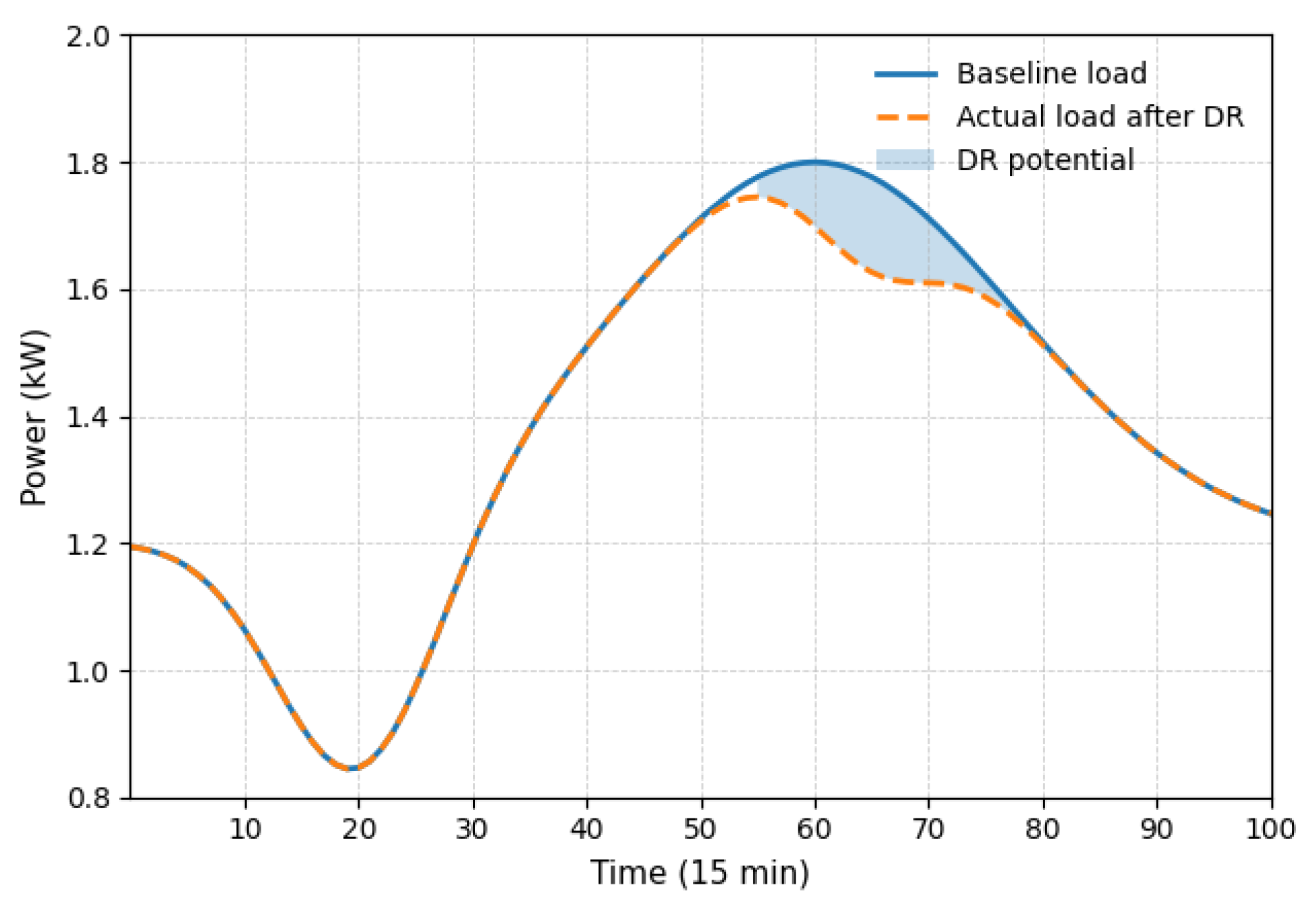
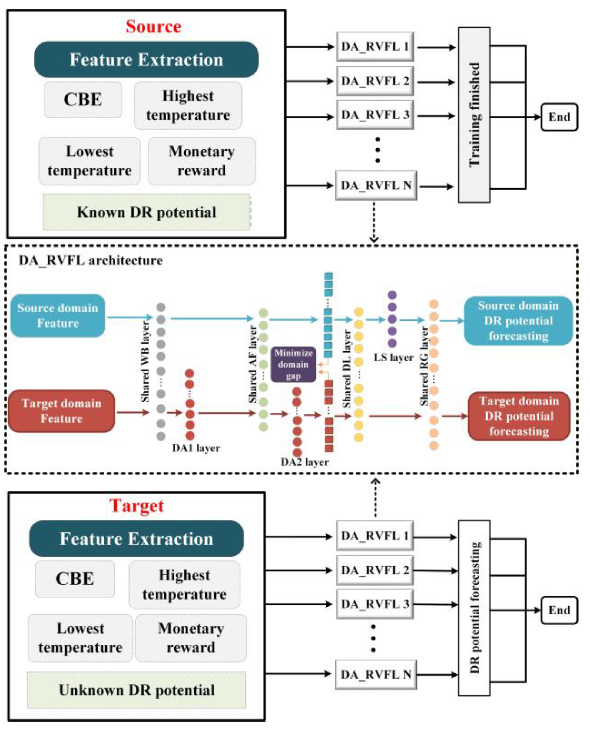
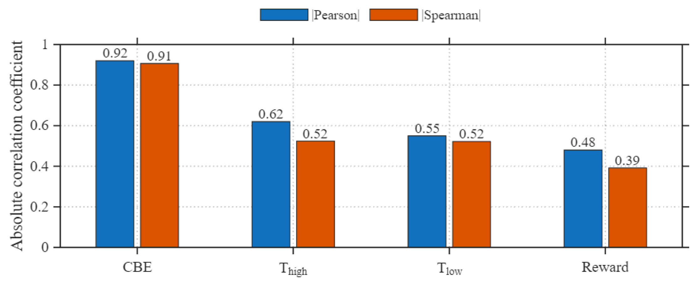
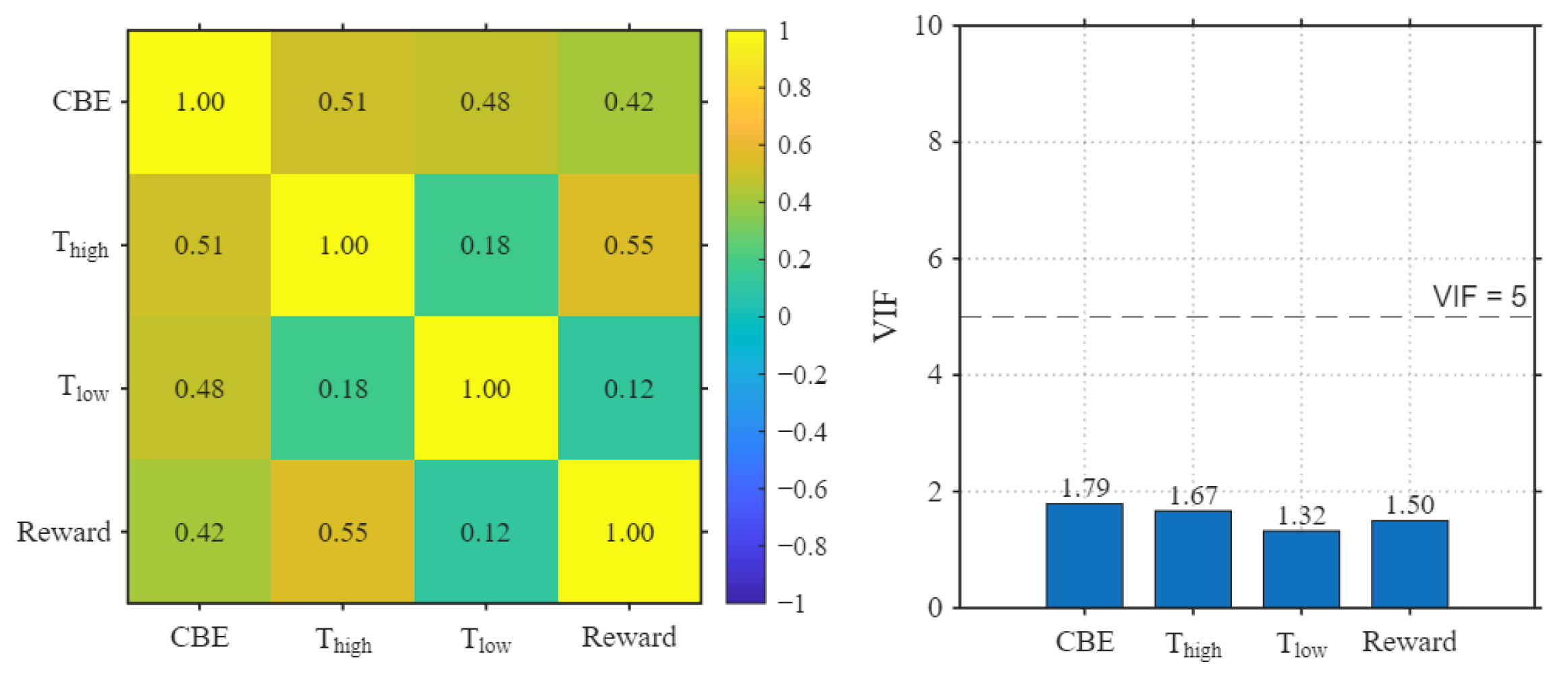
This section presents the experimental validation of the proposed framework through comprehensive case studies. The dataset construction and simulation settings are first introduced, followed by the experimental design under different source–target domain configurations. Parameter configurations, comparative results, and computational cost analyses are then provided to evaluate forecasting accuracy, robustness under distribution shifts, and practical deployability.

4.1. Data Set

The dataset used in this study is constructed based on real-world residential electricity consumption data from the Pecan Street project in Austin, TX, USA. Pecan Street provides high-resolution smart meter measurements and publicly accessible residential energy datasets [23], and has been widely adopted in studies related to residential demand response (DR), load aggregation, and energy behavior modeling. Its long-term and fine-grained data characteristics make it particularly suitable for investigating cross-domain learning problems under distributional shifts, which is the main focus of this paper. The original dataset contains 1-min resolution electricity consumption records for approximately 500 residential households, including both whole-house and appliance-level measurements. To ensure data completeness and consistency, households with missing or discontinuous records over the study period are removed. The remaining data span a continuous two-year period from 1 January 2015 to 31 December 2016, enabling the analysis of inter-annual variations in residential load patterns caused by differences in weather conditions, customer behavior, and household composition. The raw data are aggregated to a 15-min resolution, which is consistent with the temporal granularity typically used in incentive-based DR programs and day-ahead electricity market operations.

Due to the lack of publicly available datasets containing actual residential load reductions during incentive-based demand response (IBDR) events, this study adopts a home energy management system (HEMS)-based simulation framework to generate reference demand response data. The HEMS model employed in this work follows the formulation proposed in [20], which has been widely used in the literature for aggregated DR capacity modeling and forecasting.

The HEMS model simulates customers’ response behavior under IBDR programs by optimizing household appliance operation with the objective of minimizing total electricity cost, while explicitly considering monetary rewards for load reduction and penalty mechanisms for unmet DR commitments [24,25]. Residential loads are categorized into three main types: air-conditioning systems, shiftable appliances, and inelastic loads. Air-conditioning systems are modeled using simplified thermal dynamic equations with ON/OFF control, temperature setpoints, and comfort deadbands. Shiftable appliances (e.g., washing machines and dishwashers) are assumed to have flexible operating time windows and are scheduled to respond to DR signals without significantly affecting user comfort. Inelastic loads are treated as fixed and non-responsive throughout the DR event. The key parameters of the HEMS model include electricity prices, reward rates, penalty rates, DR event start times and durations, appliance rated power, and thermal characteristics of residential buildings. These parameters are summarized in

Table 2. Parameters in the dr events.

Parameter	Value
Base Electricity Price	0.3 $/kWh
Monetary Reward	0.3, 0.4, 0.5 $/kWh
DR Event Time	12:00–14:00, 17:00–20:00
Time Resolution	15 min
Customer Types	comfort-focused, cost-focused

and are consistent with typical settings adopted in residential DR studies.

It should be emphasized that the HEMS model is not newly proposed in this paper, nor is it tuned to favor the proposed forecasting method. Instead, it serves solely as an offline data generation mechanism to produce realistic and internally consistent demand response (DR) samples based on authentic residential consumption data from the Pecan Street dataset. Similar HEMS-based frameworks have been widely adopted and validated in prior studies to approximate aggregated residential customer behavior under incentive-based DR programs [13,19,20]. Although the simulated DRs cannot fully replicate real-world customer behavior in the absence of actual incentive-based DR event data, this limitation applies uniformly to all benchmark models and experimental cases considered in this study. Moreover, the same HEMS-generated DR potential values are consistently used across both the source and target domains. As a result, any modeling bias introduced by the underlying HEMS assumptions affects all methods in a consistent manner and does not compromise the fairness of the comparative evaluation or the validity of the relative performance conclusions.

From a robustness and sensitivity perspective, variations in HEMS assumptions or parameter settings primarily manifest as changes in the statistical distribution of the aggregated DR potential, rather than altering the fundamental relationship between aggregated baseline consumption, exogenous conditions, incentive signals, and response capability. Since the proposed framework does not incorporate appliance-level control logic or HEMS-specific parameters, but instead relies on domain-adaptive feature learning and marginal distribution alignment, it is inherently less sensitive to specific HEMS configurations. Consequently, moderate variations in HEMS parameters are expected to be effectively accommodated by the proposed domain-adaptive transfer learning mechanism.

4.2. Case Settings

To comprehensively evaluate the effectiveness, stability, and data-efficiency of the proposed domain-adaptive transfer learning framework, eight case studies are designed with different source–target domain configurations and source-domain data proportions.

Specifically, 55 demand response (DR) event days from the summer of 2015 are used to construct Dataset_1, while 65 DR event instances from the summer of 2016 form Dataset_2, as summarized in Table 2. Owing to inter-annual differences in weather conditions, customer composition, and consumption patterns, these two datasets naturally exhibit noticeable distributional discrepancies, making them well suited for evaluating cross-domain transfer performance. It should be noted that the demand response (DR) event days in Dataset_1 and Dataset_2 are not randomly sampled from the full two-year dataset. Instead, they are selected from predefined summer periods (June–September) in 2015 and 2016 and correspond to days with simulated incentive-based DR events generated by the HEMS model. The selected DR event days are temporally distributed within each summer period but not strictly consecutive, as they are constrained by data availability and predefined DR event settings. Focusing on summer periods may introduce a certain degree of seasonal sampling bias by over-representing weather-sensitive load behaviors, such as air-conditioning usage. However, this bias is applied consistently to both the source and target domains. Despite being drawn from the same season, Dataset_1 and Dataset_2 exhibit noticeable inter-annual distribution shifts due to differences in weather conditions, customer composition, and baseline consumption patterns, leading to discrepancies in both input feature distributions and aggregated DR potential. This setting naturally forms a cross-domain learning scenario and constitutes a key motivation for adopting a transfer learning framework in this study. Accordingly, the results should be interpreted as representative of seasonal DR scenarios, and caution should be exercised when extrapolating them to other seasons.

In practical demand response applications, load aggregators often face severe data scarcity when incorporating new customer groups or expanding into new operational regions. Historical DR data are typically available only for a small subset of customers or events, while collecting additional labeled data requires costly and time-consuming field experiments. To realistically reflect this constraint, the initial case studies (Cases 1–4) deliberately restrict the source-domain training data to 10% of the available samples. This setting represents an extreme yet practically relevant scenario and is intended to assess the lower bound of data availability under which effective transfer learning can still be achieved. Under this design, the target domain is assumed to be completely unlabeled, and no target-domain information is used during model training or hyperparameter tuning. This strict separation ensures that the evaluation faithfully reflects a real-world deployment scenario for unlabeled target domains.

To further examine the robustness and stability of the proposed framework with respect to the amount of source-domain data, four additional cases (Cases 5–8) are introduced by increasing the source-domain proportion to 20% and 30%, respectively. These cases enable a systematic sensitivity analysis that evaluates whether the model’s performance trends remain consistent as more source-domain information becomes available.

Across all cases, the remaining samples in the corresponding dataset are used exclusively for testing. For intra-year scenarios (Cases 1 and 2), the source and target domains are drawn from the same dataset, while for cross-year scenarios (Cases 3–8), the source and target domains are drawn from different years to introduce more pronounced distribution shifts. The complete experimental configuration is summarized in

Table 3. Summary of Test Methods.

Case Study	Source Domain	Target Domain
Case 1	10% from Dataset_1	90% from Dataset_1
Case 2	10% from Dataset_2	90% from Dataset_2
Case 3	10% from Dataset_1	100% from Dataset_2
Case 4	10% from Dataset_2	100% from Dataset_1
Case 5	20% from Dataset_1	100% from Dataset_2
Case 6	20% from Dataset_2	100% from Dataset_1
Case 7	30% from Dataset_1	100% from Dataset_2
Case 8	30% from Dataset _2	100% from Dataset _1

. This multi-case experimental setup provides a rigorous and transparent basis for evaluating the practical applicability of the proposed framework in real-world demand response environments characterized by limited labeled data and evolving customer behavior.

From an operational perspective, the case settings in this study are designed to reflect realistic deployment conditions faced by load aggregators. In practice, forecasting models for aggregated demand response (DR) potential are typically trained offline using historical data and updated periodically as new data become available, rather than being retrained in real time. Accordingly, all models in this study are trained under an offline learning setting, and their computational cost is evaluated to assess practical feasibility.

As will be shown in Section 4.4, the proposed DA-RVFL framework exhibits training and inference times that are comparable to conventional machine learning models such as RF and SVR, and substantially lower than deep learning-based LSTM models. This is mainly due to the closed-form least-squares optimization and the absence of iterative backpropagation. All experiments are conducted in a CPU-based environment, indicating that the proposed approach can be readily implemented by load aggregators without requiring specialized hardware or cloud-scale computing resources. These characteristics make the proposed framework suitable for routine operational use in day-ahead bidding and planning scenarios.

Although the forecasting accuracy in this study is evaluated using statistical metrics such as RMSE and MAPE, these improvements have direct operational and economic implications for load aggregators. More accurate prediction of aggregated DR potential reduces the likelihood of overestimating available flexibility, which in turn lowers the risk of failing to meet committed DR bids and incurring penalty costs. At the same time, improved accuracy mitigates underestimation of DR capability, enabling aggregators to submit more competitive bids and fully utilize available demand-side flexibility. Therefore, the observed reductions in RMSE and MAPE translate into lower supply risk, more reliable DR participation, and improved economic efficiency in market operations. While a detailed market-level economic analysis is beyond the scope of this paper, the consistent accuracy improvements demonstrated across multiple case studies indicate tangible practical benefits for real-world aggregator decision-making.

4.3. Parameter Configuration

To simultaneously preserve predictive accuracy on the source domain and promote domain-invariant feature learning, the final loss function $L_{\mathrm{total}}$ is constructed. It explicitly combines the DA-RVFL training loss-defined as the root mean square error (RMSE) on the source-domain data-with a Maximum Mean Discrepancy (MMD) loss term applied to the outputs of the DL layer for both the source and target domains.

$$\min L_{\mathrm{tot}al}=L_{rmse}+{\lambda }_{\mathrm{mm}d}{L}_{mmd}$$

(16)

where $L_{\mathrm{m}\mathrm{m}\mathrm{d}}$ quantifies the distributional divergence $Dist\left(X^S,X^t\right)$ between the source and target datasets, and ${ \lambda }_{\mathrm{m}\mathrm{m}\mathrm{d}}$ is a hyperparameter that balances the contribution of the primary DA-RVFL training loss against the domain adaptation loss. Once this objective function is formulated, the model parameters can be optimized to automatically minimize the distribution discrepancy between the source and target domains during training. In this study, the hyperparameter ${ \lambda }_{\mathrm{m}\mathrm{m}\mathrm{d}}$ is selected through empirical tuning using a validation subset of the source-domain data. Values of ${ \lambda }_{\mathrm{m}\mathrm{m}\mathrm{d}}$ in the range [0.01, 1] are evaluated, and the model performance is observed to be relatively stable within this interval. Based on this analysis, ${ \lambda }_{\mathrm{m}\mathrm{m}\mathrm{d}}$ is fixed at 0.1 for all experiments, as it provides a favorable balance between forecasting accuracy and domain adaptation effectiveness.

The methodological setup of the ensemble model involves several key hyperparameters designed to balance predictive performance and computational complexity. To encourage diverse feature representations, the number of hidden-layer nodes is constrained to the range of 400–600. In addition, an ensemble consisting of 200 independent DA-RVFL models is constructed, representing a practical compromise between improved predictive accuracy and computational cost. The sigmoid function is adopted as the activation function throughout the network.

4.4. Results and Analysis

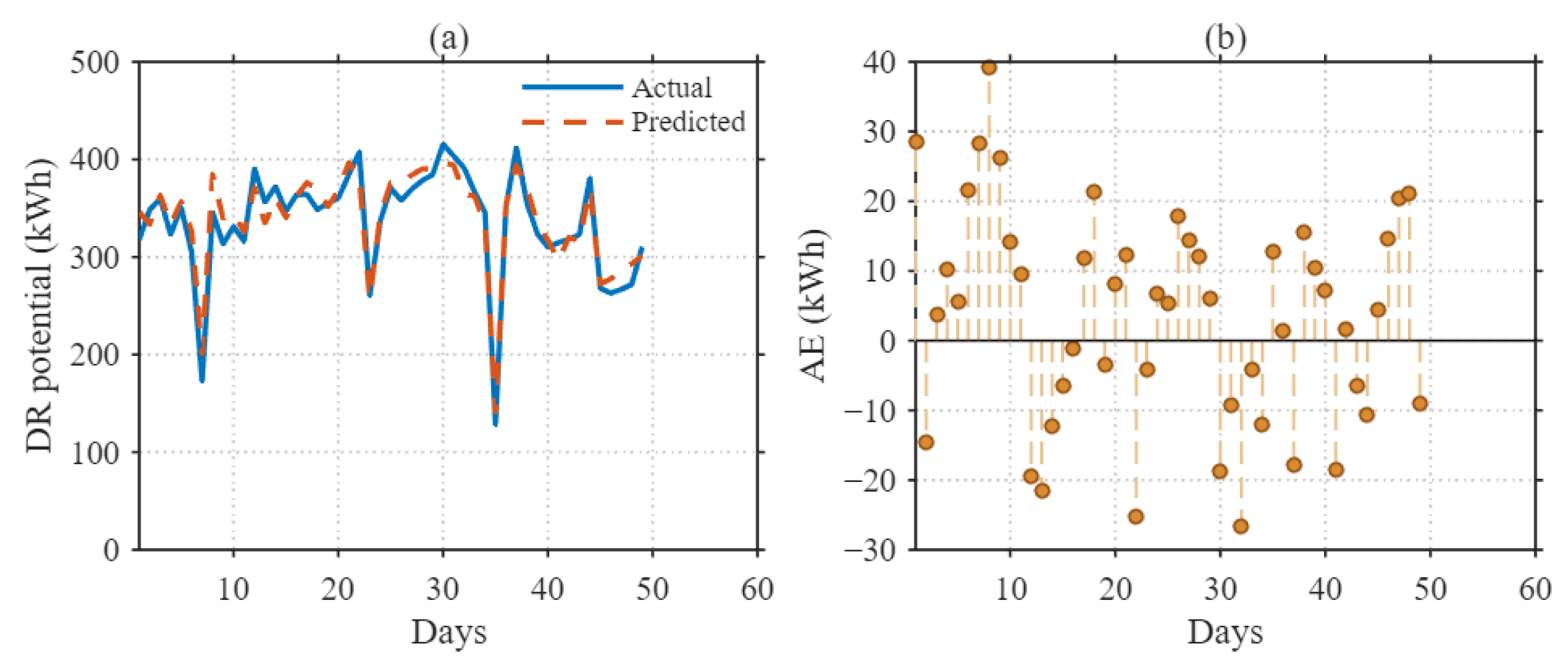
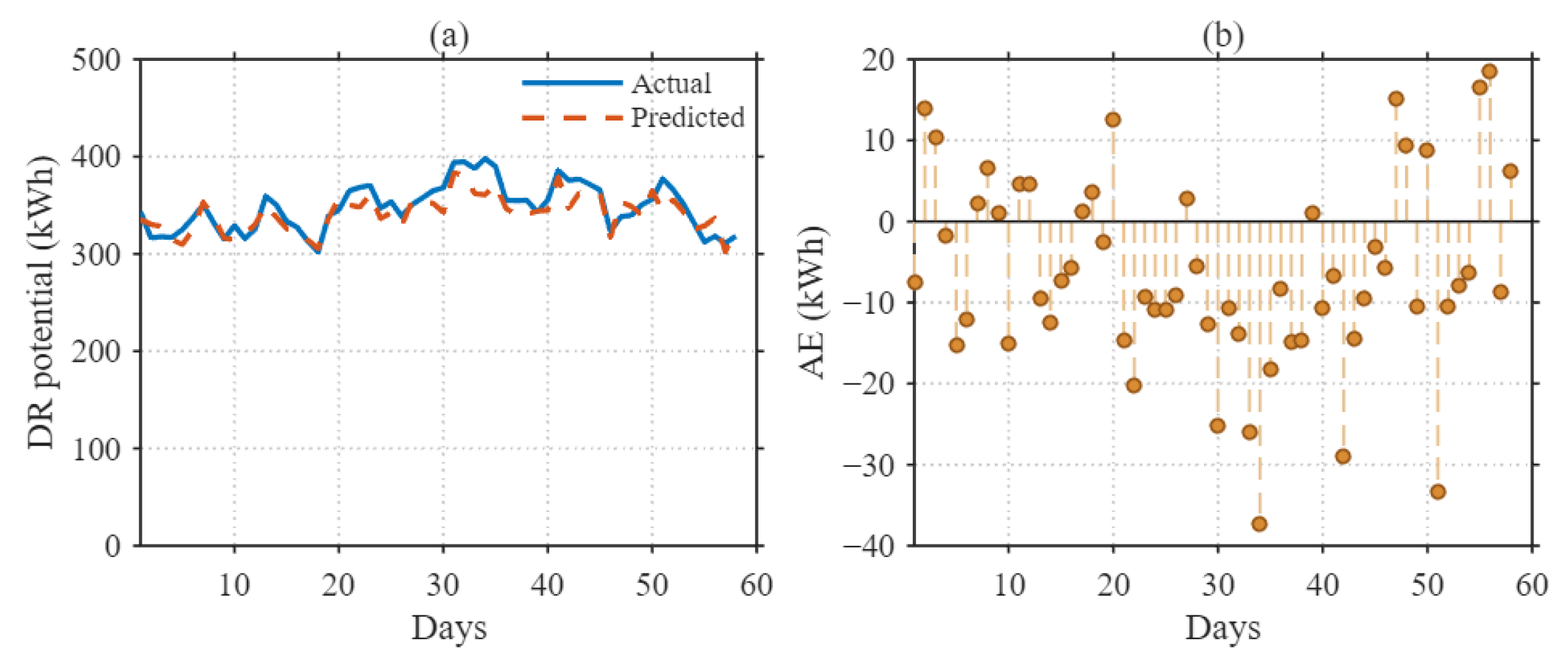
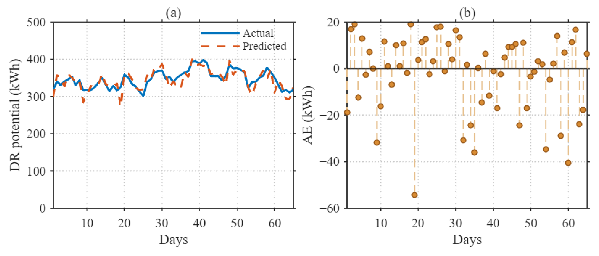
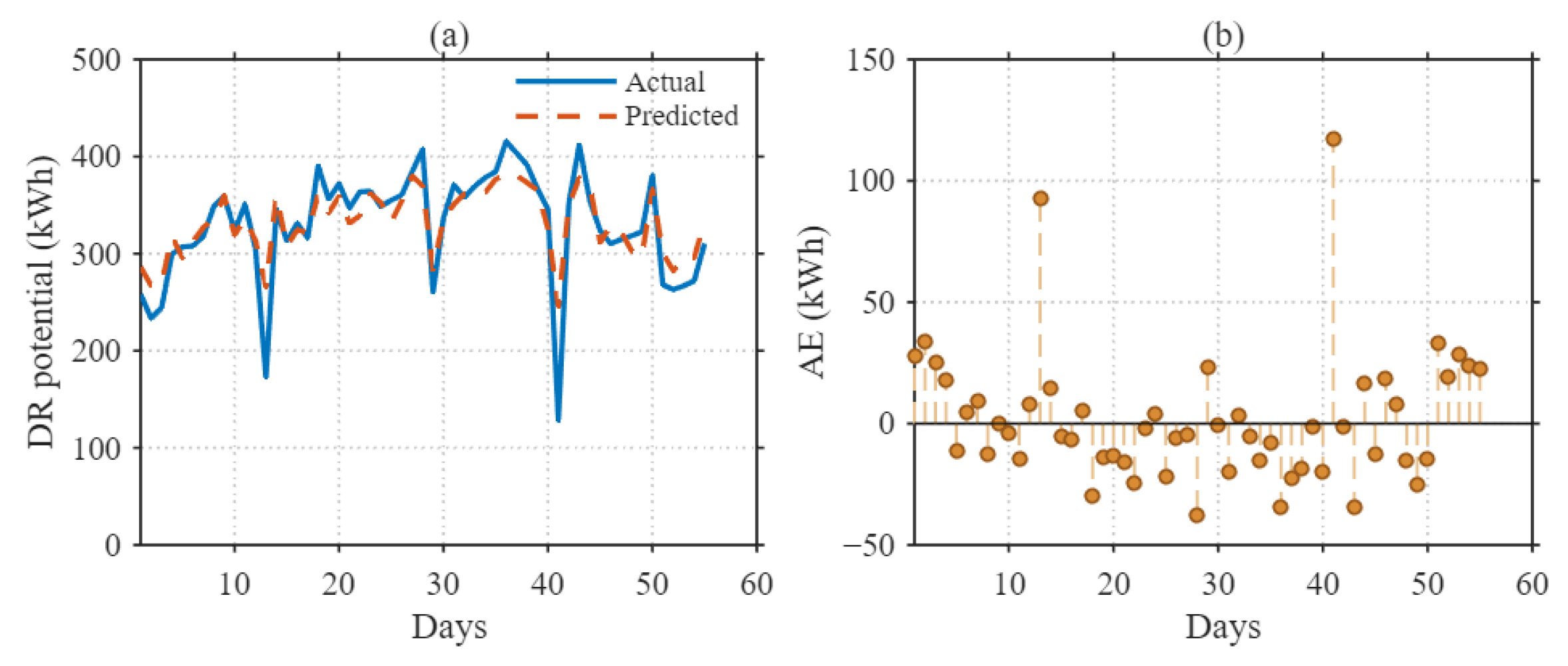
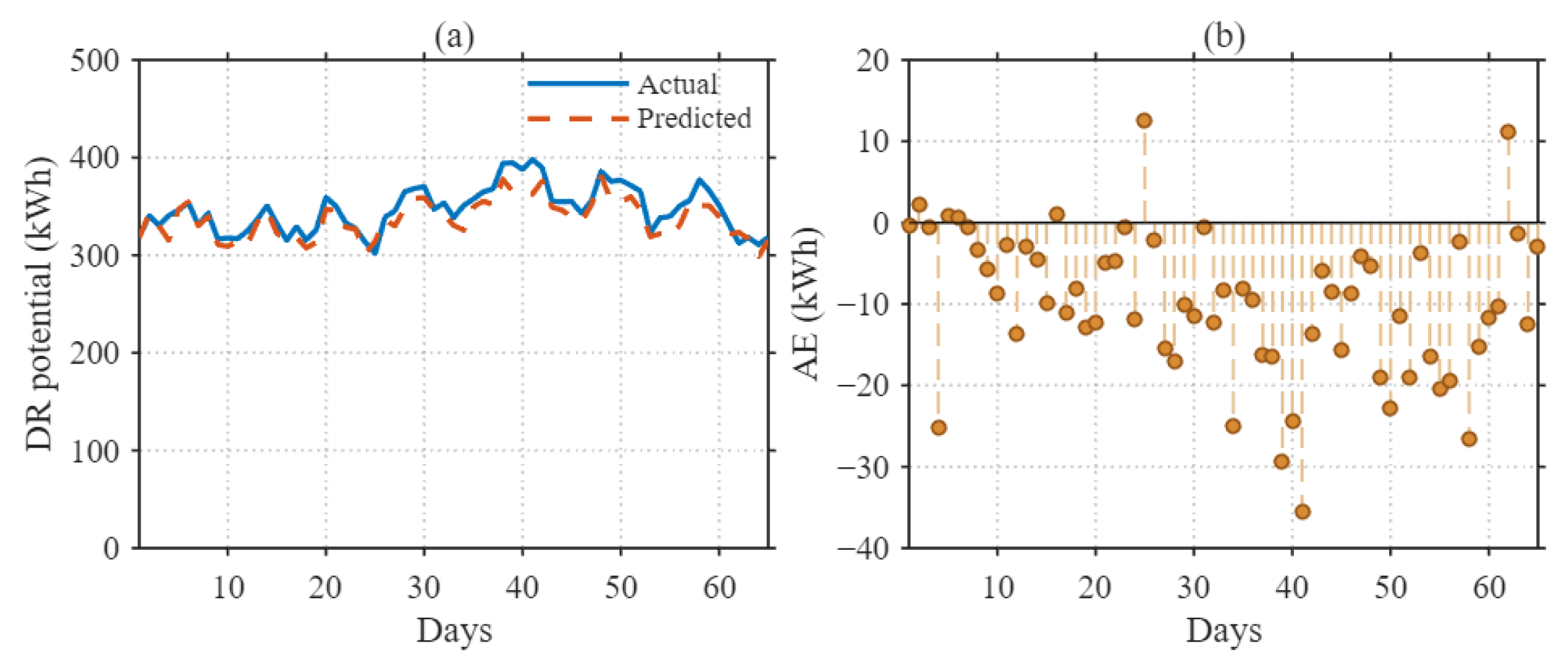
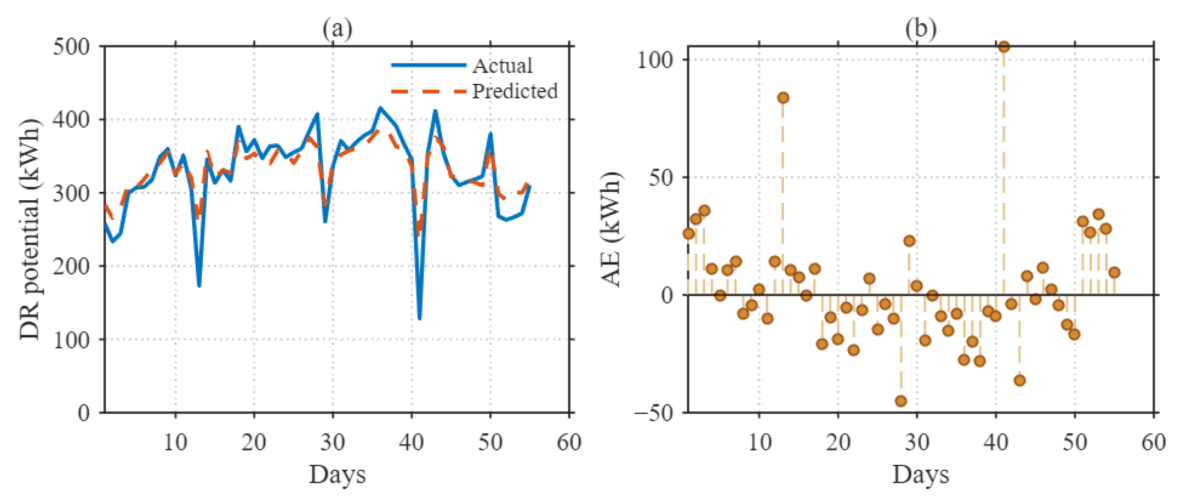
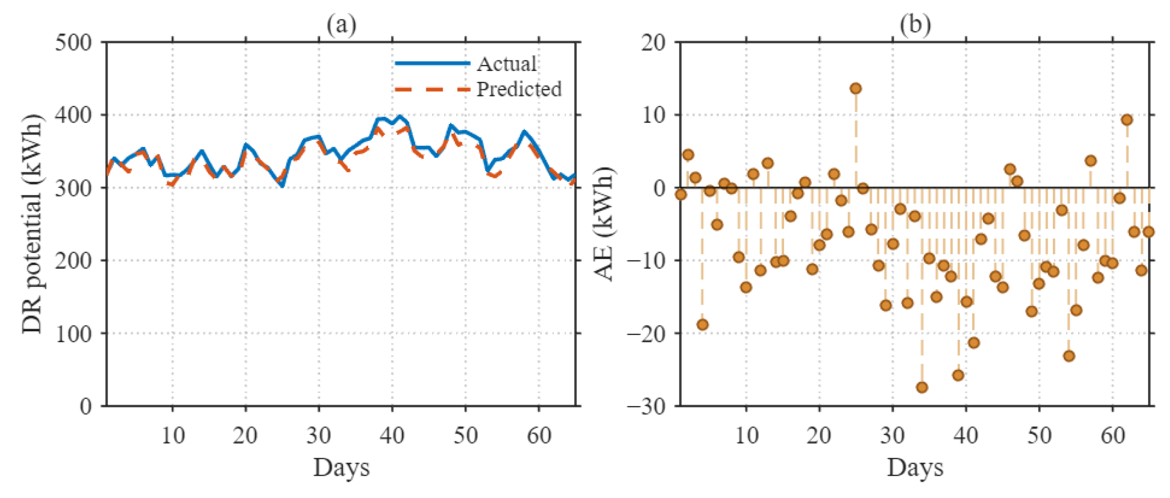
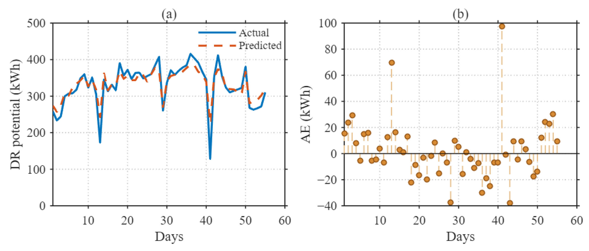
Figure 6, Figure 7, Figure 8, Figure 9, Figure 10, Figure 11, Figure 12 and Figure 13 present the temporal prediction results of the aggregated demand response (DR) potential for all eight case studies. Cases 1–4 correspond to the extreme low-data scenario where only 10% of the source-domain samples are available, while Cases 5–8 progressively increase the source-domain proportion to 20% and 30%.

As shown in Figure 6, Figure 7, Figure 8 and Figure 9, the predicted DR potential closely follows the actual temporal dynamics in both intra-year (Cases 1 and 2) and cross-year (Cases 3 and 4) transfer scenarios. Despite the pronounced distribution mismatch introduced by inter-annual variations in weather conditions and customer behavior, the proposed method maintains stable tracking performance and avoids the large deviations observed in conventional machine learning models. Quantitatively,

Table 4. Comparison of forecasting performance in terms of Root mean square error (RMSE), Mean absolute percentage error (MAPE), and Coefficient of determination (R²). (Note: The best performance in each column is highlighted in bold).

Metric	Method	Case 1	Case 2	Case 3	Case 4	Case5	Case6	Case7	Case8
RMSE	RF	68.4046	22.9207	63.2621	52.2106	29.6539	50.3406	25.7318	42.0382
	SVR	46.8428	19.1809	43.0615	53.0753	26.4250	43.5429	15.8267	36.7840
	LSTM	29.3842	18.6068	28.2521	43.0811	23.4844	41.8536	16.5501	36.2345
	Proposed	16.2196	13.5175	16.4483	28.0326	13.1854	25.9948	10.5804	22.7491
MAPE	RF	0.2063	0.0536	0.2046	0.1086	0.0775	0.1063	0.0646	0.0712
	SVR	0.130	0.0412	0.1209	0.1020	0.0634	0.0991	0.0360	0.0594
	LSTM	0.0683	0.0405	0.0760	0.0797	0.0573	0.0705	0.0405	0.0618
	Proposed	0.0407	0.0324	0.0382	0.0616	0.0311	0.0568	0.0252	0.0502
R2	RF	−0.5786	0.1048	−6.3147	0.1254	−0.1063	0.1869	−0.2102	0.3948
	SVR	0.2598	0.3731	−2.3891	0.0962	−0.2763	0.3971	0.5422	0.5659
	LSTM	0.7087	0.4101	−0.4588	0.4045	−0.0080	−0.3859	0.4994	−0.2812
	Proposed	0.9112	0.6887	0.5055	0.7479	0.6822	0.7840	0.7953	0.8340

shows that the proposed method consistently achieves the lowest RMSE and MAPE values and the highest coefficient of determination (R²) across all four cases. In particular, for the most challenging cross-year transfer scenario (Case 3), the proposed framework improves RMSE by more than 40% compared with LSTM and by an even larger margin compared with RF and SVR. 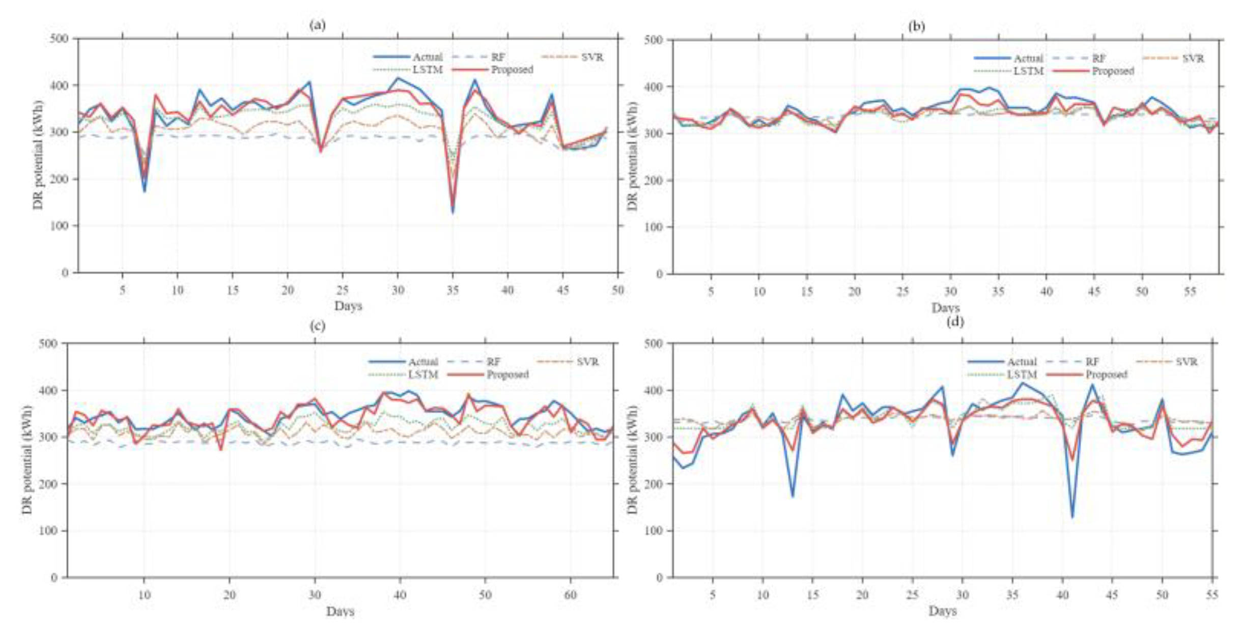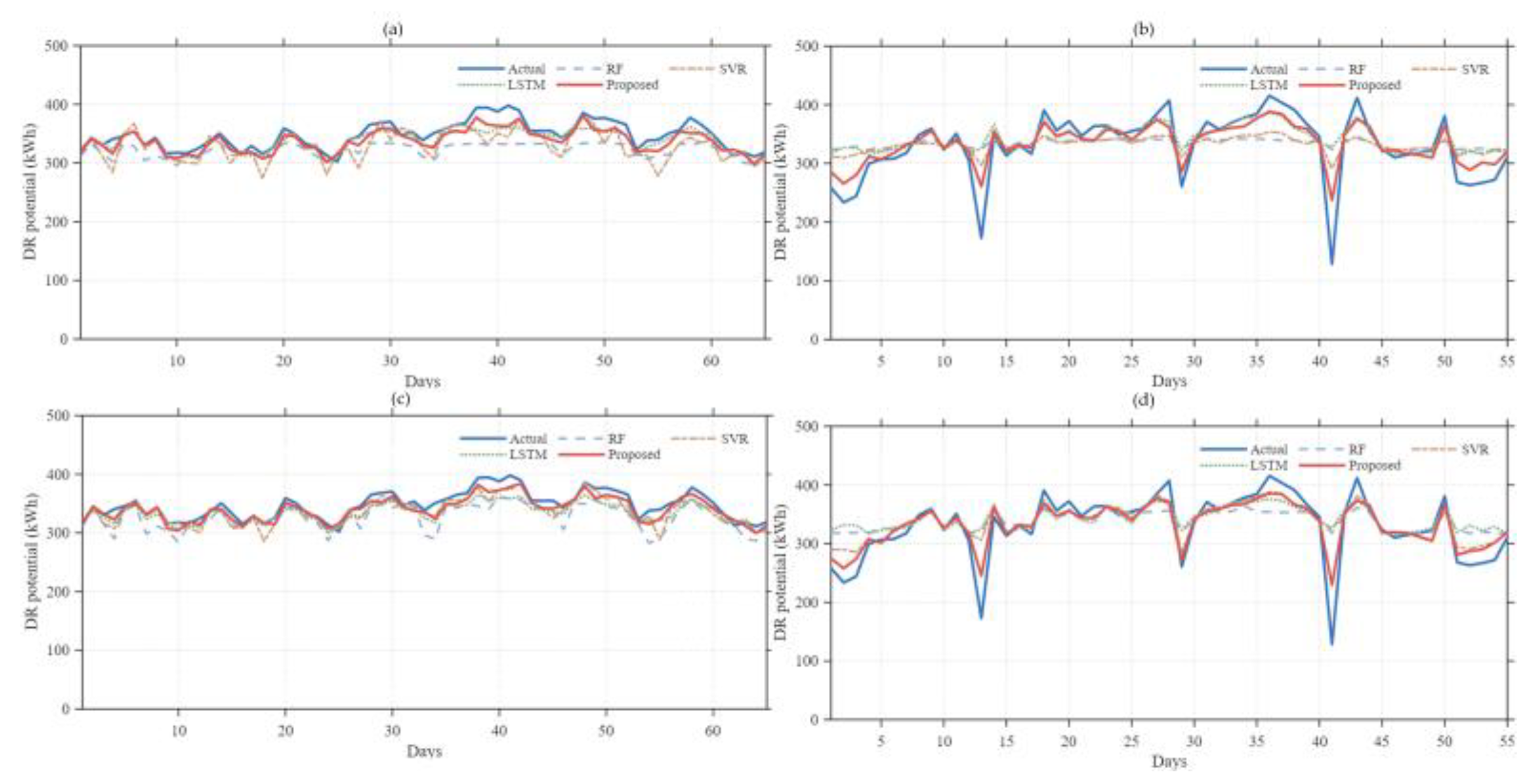The relatively high R² values (above 0.5 in all cases) further indicate that the proposed model captures the dominant variation patterns of aggregated DR potential, whereas several benchmark models exhibit near-zero or even negative R² values, reflecting their inability to generalize under severe data scarcity. These results confirm that the proposed framework is not merely fitting the source-domain data but is able to extract domain-invariant representations that remain effective when transferred to unlabeled and distribution-shifted target domains. In Cases 5–8 extend the analysis by increasing the proportion of source-domain data to 20% and 30%, respectively. This design explicitly evaluates the sensitivity of the proposed method to the size of the source-domain training set and assesses whether the performance gains observed at 10% remain consistent or improve systematically as more data become available. As illustrated in Figure 10, Figure 11, Figure 12 and Figure 13 and summarized in Table 4, increasing the source-domain proportion leads to a monotonic reduction in RMSE and MAPE for the proposed method in both transfer directions (Dataset_1 → Dataset_2 and Dataset_2 → Dataset_1). For example, in the Dataset_1 → Dataset_2 transfer setting, RMSE decreases from 16.45 (Case 3, 10%) to 13.19 (Case 5, 20%) and further to 10.58 (Case 7, 30%). A similar trend is observed for MAPE and R², with R² increasing steadily and exceeding 0.79 in Case 7.

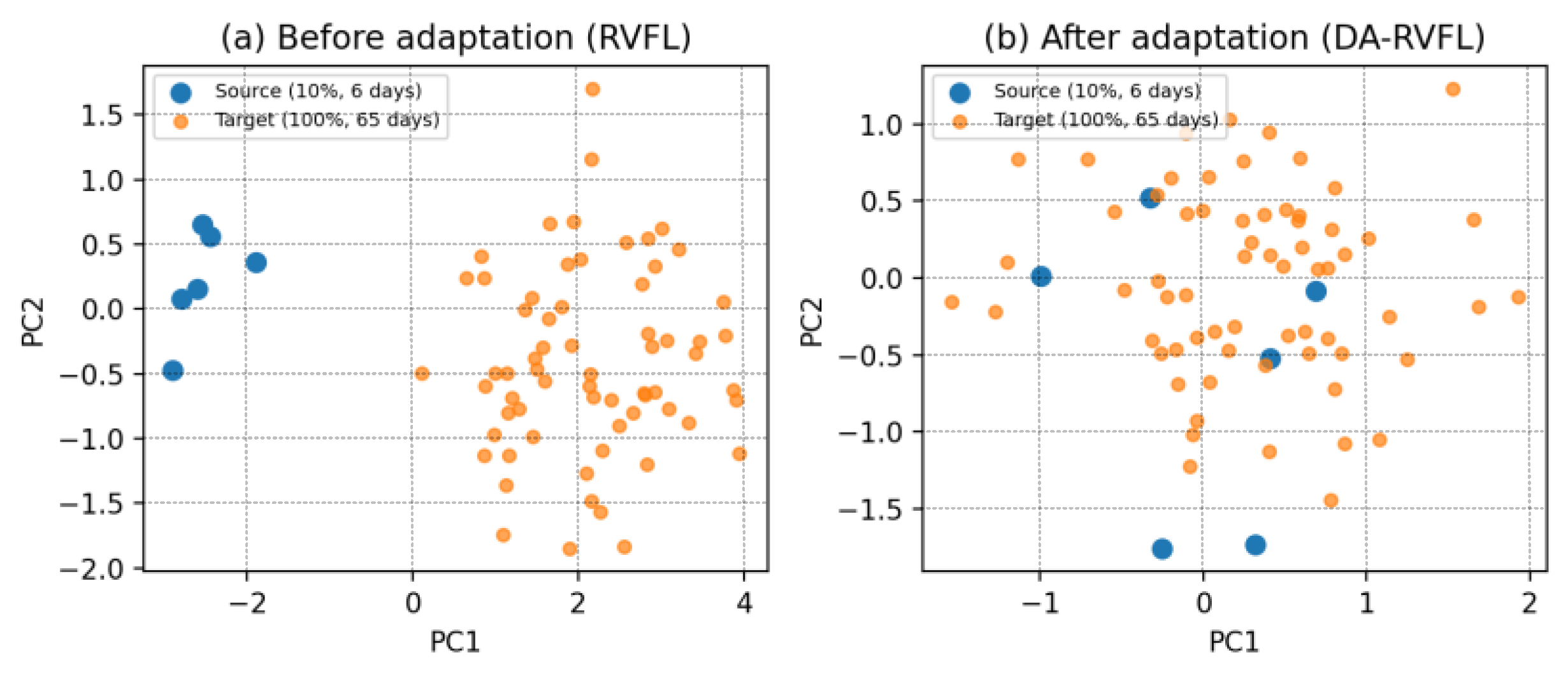
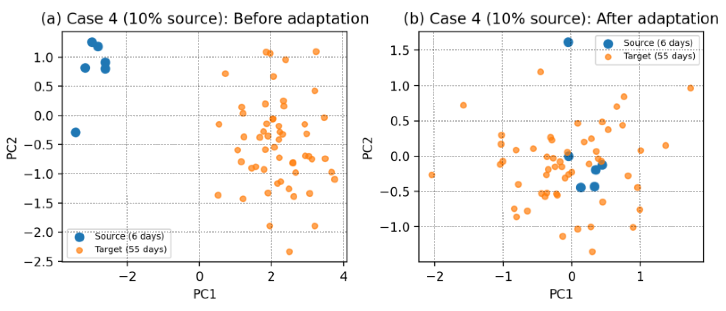
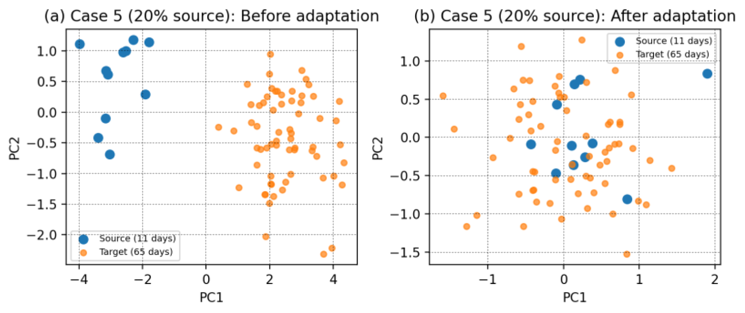
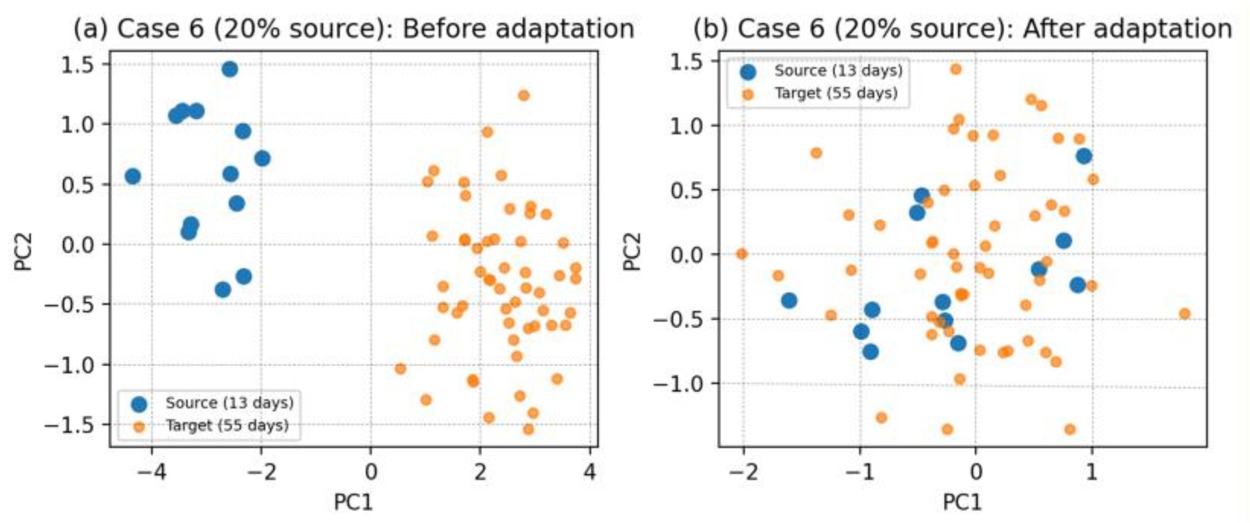
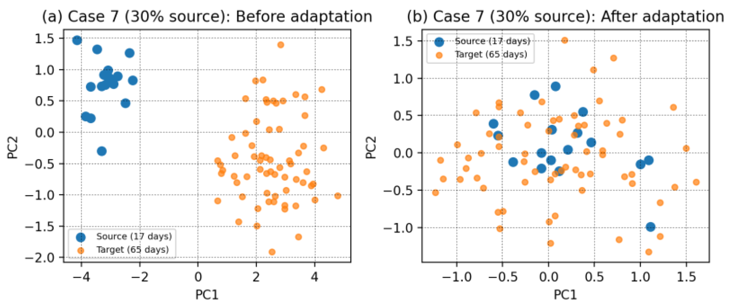
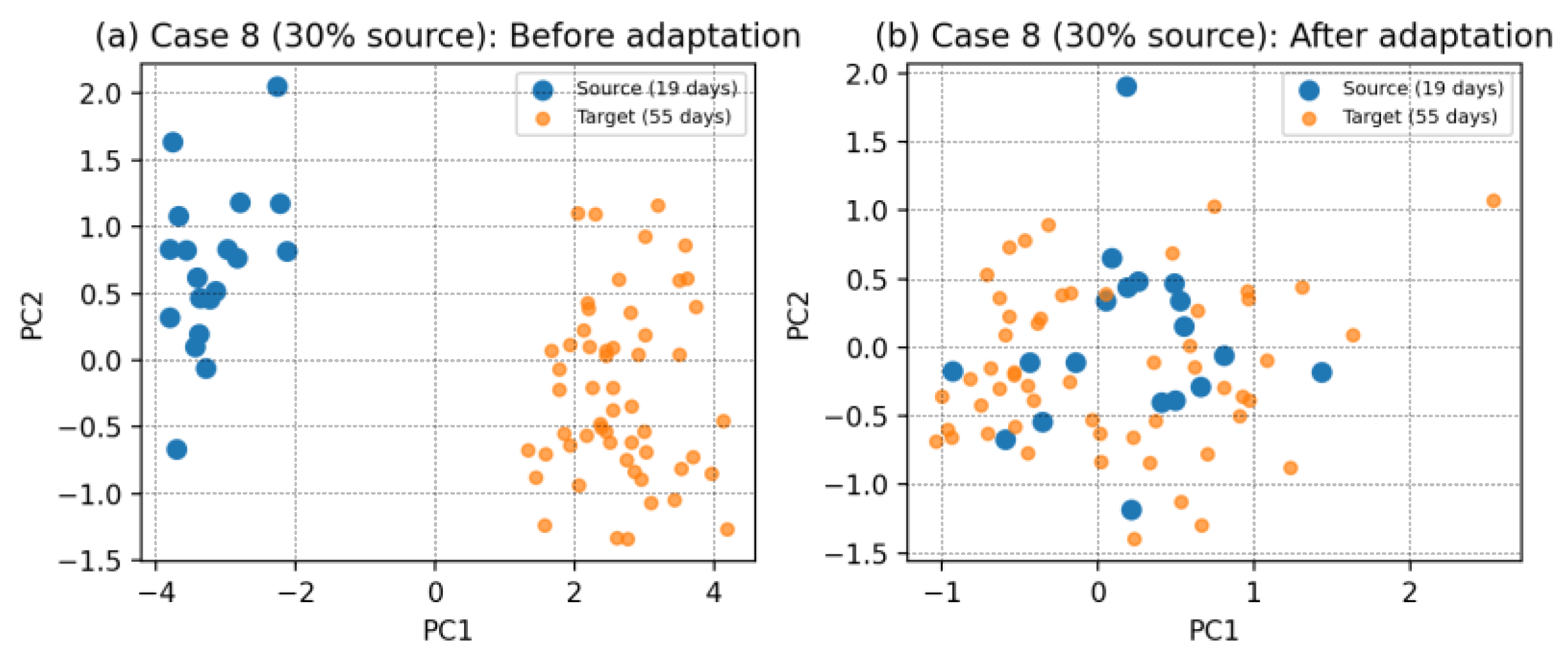
To further investigate the mechanism underlying the performance improvements observed in cross-year transfer scenarios, the latent feature distributions before and after domain adaptation are visualized using principal component analysis (PCA) for Cases 3–6, as shown in Figure 14, Figure 15, Figure 16, Figure 17, Figure 18 and Figure 19. These cases represent challenging settings with pronounced inter-annual distribution shifts and limited source-domain data availability. In the absence of domain adaptation, the latent representations learned by the standard RVFL model exhibit clear separation between the source and target domains across all cases, indicating substantial distribution mismatch caused by differences in weather conditions, customer composition, and baseline consumption patterns between years. This separation is particularly evident in Cases 3 and 4, where only 10% of the source-domain data are available, highlighting the difficulty of cross-domain generalization under severe data scarcity.

To ensure a fair and meaningful comparison, all benchmark methods considered in this study were carefully optimized and tuned using only source-domain data prior to performance evaluation. A consistent validation procedure was applied across all models to determine appropriate hyperparameter settings, with the objective of achieving their best possible predictive performance under each case study. This unified tuning strategy avoids bias introduced by uneven optimization efforts and ensures that the observed performance differences genuinely reflect the intrinsic modeling capability of each approach. The detailed hyperparameter configurations of the compared methods are summarized as follows.

• The support vector regression (SVR) model employed a radial basis function (RBF) kernel. The regularization parameter C, kernel width parameter $\gamma$, and insensitive loss parameter $\epsilon$ were selected using a grid search combined with five-fold cross-validation. The search ranges were $C\in \{1,5,10\}$, $\gamma \in \{0.001,0.01,0.1\}$, and $\epsilon \in \{0.05,0.1,0.2\}$. The final configuration ($C=5.0$, $\gamma =0.01$, $\epsilon =0.1$) achieved the lowest validation RMSE.
• The random forest (RF) hyperparameters, including the number of trees, maximum tree depth, minimum number of samples required to split an internal node, and minimum number of samples per leaf, were tuned using cross-validation. The final configuration—200 trees, a maximum depth of 10, a minimum split size of 5, and a minimum leaf size of 2—was selected based on its superior validation performance while maintaining model robustness.
• The hyperparameters of the long short-term memory (LSTM) model were determined using a combination of grid search and validation-based early stopping. The number of hidden units {30, 50, 80}, dropout rate {0.1, 0.2, 0.3}, and learning rate {0.0005, 0.001} were evaluated. The final architecture consisted of 50 LSTM units with a dropout rate of 0.2, trained using a learning rate of 0.001 and a batch size of 30. Training was terminated when the validation loss converged to prevent overfitting.

After the above hyperparameter configuration and validation procedure, all benchmark models (SVR, RF, and LSTM) were re-trained using the selected optimal settings on the corresponding source-domain training set and then evaluated on the target-domain test set in each case study. This ensures that performance differences among methods originate from their generalization capability under data scarcity and domain shift, rather than from suboptimal tuning. The comparative results are reported quantitatively in Table 3 and further illustrated in Figure 20, Figure 21, Figure 22 and Figure 23, which collectively provide a clear assessment of prediction accuracy (RMSE and MAPE) and goodness-of-fit (R²) across different transfer scenarios and source-data proportions.

After applying the proposed DA-RVFL framework, the latent feature distributions of the source and target domains become substantially more aligned in all cases. Notably, effective alignment is achieved even when the source domain contains only a small number of DR event days (Cases 3 and 4), demonstrating the strong data efficiency and robustness of the proposed domain adaptation mechanism. As the proportion of source-domain data increases to 20% (Cases 5 and 6), the alignment becomes more stable and compact, which is consistent with the monotonic improvements observed in the quantitative performance metrics.

Overall, these latent-space visualizations provide intuitive evidence that the proposed DA-RVFL framework effectively mitigates inter-annual distribution shifts at the representation level, enabling reliable knowledge transfer from a limited source domain to an unlabeled target domain. This explains the superior forecasting performance achieved by the proposed method in cross-year demand response potential prediction under realistic data scarcity conditions.

More specifically, for each case study, the source-domain data used for training were further partitioned into training and validation subsets using a five-fold cross-validation strategy. The hyperparameters of all baseline models were determined exclusively based on the source-domain data, without incorporating any target-domain information, in order to strictly adhere to the unlabeled target-domain assumption of the transfer learning setting. This experimental design ensures a fair and unbiased comparison among different algorithms under identical data availability and domain-shift conditions.

The support vector regression (SVR) model employed a radial basis function (RBF) kernel. Although SVR demonstrates reasonable performance in several intra-year scenarios, its prediction accuracy degrades noticeably in cross-year transfer cases. As shown in Table 4, SVR yields relatively high RMSE and MAPE values in Cases 3 and 4, accompanied by negative or low R² values. This behavior indicates that SVR is sensitive to distribution shifts and struggles to generalize when the statistical characteristics of the target domain differ substantially from those of the source domain. The random forest (RF) model exhibits the weakest overall performance among the benchmark methods. Despite its robustness to noise and its ability to capture nonlinear relationships, RF relies heavily on sufficient and representative training data. Under severe data scarcity and domain mismatch conditions, RF fails to construct reliable decision boundaries, resulting in large prediction errors and highly unstable R² values. In several cross-domain cases, negative R² values are observed, suggesting that RF predictions are inferior to naive mean-based estimates. This limitation is particularly evident in Cases 1 and 3, where the combination of limited source-domain data and strong distribution shifts significantly undermines model generalization. The long short-term memory (LSTM) model generally outperforms RF and SVR in scenarios where temporal dependencies can be effectively learned. In intra-year cases with relatively mild distribution differences, LSTM achieves moderate prediction accuracy. However, its performance deteriorates substantially in cross-year transfer scenarios. As indicated in Table 4, LSTM yields unstable R² values and elevated RMSE in Cases 3, 6, and 8. This behavior can be attributed to the strong data dependency of deep learning models: when training samples are limited and the target-domain distribution deviates from the source domain, LSTM tends to overfit the source-domain temporal patterns and fails to generalize to unseen conditions.

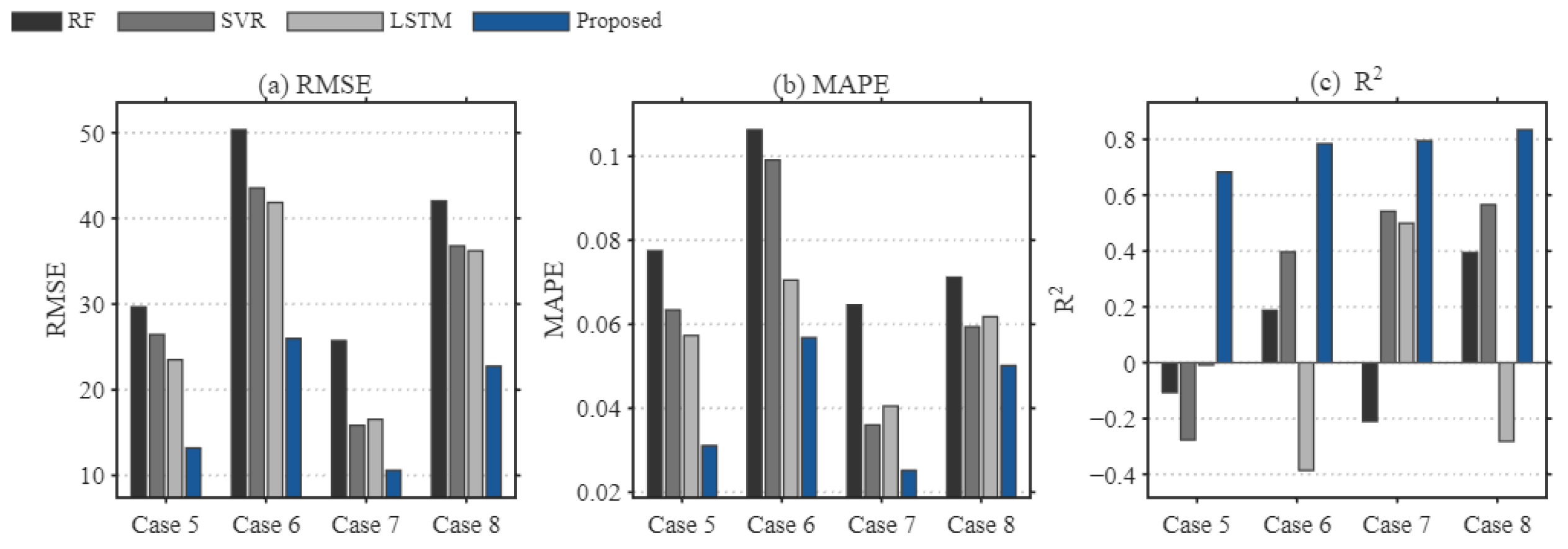
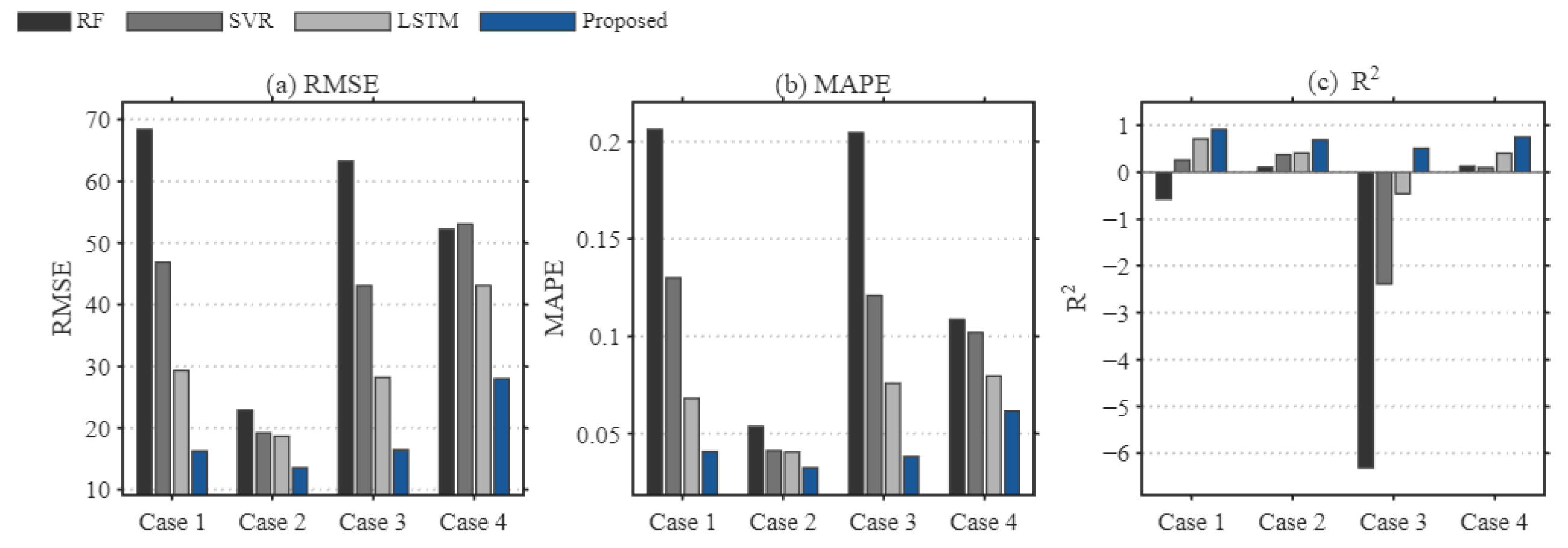
In contrast, the proposed DA-RVFL framework consistently achieves superior performance across all evaluation metrics and case studies. As summarized in Table 4 and illustrated in Figure 20, Figure 21, Figure 22 and Figure 23, the proposed method yields the lowest RMSE and MAPE values and the highest R² values in all eight cases. Notably, its performance advantage is particularly pronounced in cross-year transfer scenarios, where traditional machine learning models experience significant degradation. This indicates that the proposed framework effectively mitigates the adverse effects of distribution mismatch through explicit domain adaptation. Figure 20 and Figure 21 provide an aggregated comparison of RMSE, MAPE, and R² across representative cases, clearly illustrating the consistent performance gap between the proposed method and the benchmark algorithms. Furthermore, the temporal prediction results shown in Figure 22 and Figure 23 demonstrate that the proposed framework is able to closely track the actual DR potential dynamics, while benchmark methods exhibit larger fluctuations and systematic biases, especially during periods of rapid load variation.

Table 5. Computational cost and training strategy comparison.

Case	Method	Training Time (s)	Testing Time (s)
Case 1	RF	15.0	4.12
	SVR	12.29	3.62
	LSTM	115.4	26.9
	Proposed	18.6	5.20
Case 2	RF	15.8	4.18
	SVR	13.1	3.68
	LSTM	118.6	27.3
	Proposed	19.4	5.28
Case 3	RF	16.2	4.21
	SVR	13.8	3.71
	LSTM	121.9	27.8
	Proposed	20.1	5.35
Case 4	RF	16.9	4.26
	SVR	14.6	3.75
	LSTM	125.4	28.2
	Proposed	21.0	5.41
Case 5	RF	19.3	4.33
	SVR	16.8	3.82
	LSTM	142.7	29.6
	Proposed	24.6	5.58
Case 6	RF	20.1	4.38
	SVR	17.6	3.87
	LSTM	148.9	30.1
	Proposed	25.8	5.64
Case 7	RF	23.4	4.45
	SVR	20.2	3.95
	LSTM	168.3	31.4
	Proposed	29.7	5.82
Case 8	RF	24.1	4.51
	SVR	21.0	4.01
	LSTM	173.6	31.9
	Proposed	31.2	5.90

reports the computational cost of different forecasting methods under all eight case studies, together with their corresponding training strategies. The results provide a quantitative assessment of the practical deployability of the proposed framework and directly complement the prediction accuracy analysis presented in Table 3. All experiments were implemented in MATLAB R2025a. The test system was equipped with an Intel Core i5-7500U CPU operating at 3.40 GHz and 8.00 GB of installed RAM. All computational cost evaluations were conducted in a CPU-based environment. First, for all methods, the training time increases monotonically from Case 1 to Case 8, which is consistent with the gradual increase in the amount of source-domain training data from 10% to 30%.

This trend confirms that the reported computational costs follow expected scalability behavior rather than being dominated by implementation artifacts. Second, traditional machine learning models, including RF, SVR, and the proposed DA-RVFL, exhibit comparable computational costs across all cases. Although the proposed method introduces additional regularization and an MMD-based domain adaptation term into the objective function, its training time remains in the same order of magnitude as RF and SVR. This is mainly because the DA-RVFL framework relies on closed-form least-squares optimization and avoids iterative backpropagation, thereby preventing excessive computational overhead. Third, compared with deep learning-based LSTM models, the proposed approach demonstrates a clear advantage in computational efficiency. While the training time of LSTM increases substantially with sample size due to its iterative sequence modeling and gradient-based optimization, the DA-RVFL framework maintains a moderate and predictable growth rate. This property is particularly important for load aggregators, who often need to retrain forecasting models repeatedly under changing customer compositions and operating conditions. Finally, the testing time of RF, SVR, and DA-RVFL remains nearly constant across all cases, indicating that the inference complexity of the proposed method is not sensitive to training data size. Although DA-RVFL incurs a slightly higher testing cost than RF and SVR due to the ensemble structure, the absolute inference time remains within a few seconds, which is well suited for day-ahead and near-real-time demand response applications. Overall, the results in Table 4 demonstrate that the proposed DA-RVFL framework achieves improved transfer learning performance (as shown in Table 3) without sacrificing computational efficiency.

5. Conclusions

This paper proposes a domain-adaptive transfer learning framework based on Random Vector Functional-Link (RVFL) neural networks for aggregated demand response (DR) potential forecasting under severe data scarcity conditions. By explicitly minimizing marginal feature distribution discrepancies between source and target domains through Maximum Mean Discrepancy (MMD) regularization, the proposed framework enables accurate DR potential prediction without requiring any labeled target-domain data. Extensive case studies based on real residential consumption data demonstrate that the proposed DA-RVFL framework consistently outperforms benchmark methods, including SVR, RF, and LSTM, across both intra-year and cross-year transfer scenarios. Reliable forecasting performance is achieved even when only 10% of the source-domain data are available, reflecting practical deployment conditions faced by load aggregators, while increasing source-domain proportions further lead to stable and monotonic accuracy improvements.

From an operational perspective, improved forecasting accuracy directly enhances the reliability of day-ahead DR bidding decisions. More accurate estimation of aggregated DR potential reduces the risk of over-commitment and associated penalty exposure, while mitigating conservative underestimation that may result in unrealized revenue opportunities. Combined with its offline training paradigm and moderate computational cost, the proposed framework can be readily integrated into existing aggregator decision-support systems without requiring specialized hardware, making it suitable for routine operational use.

Despite these advantages, several limitations should be acknowledged. The proposed framework primarily aligns marginal feature distributions and assumes relative stability in the conditional relationship between input features and aggregated DR potential, which may be challenged under abrupt behavioral changes, extreme weather conditions, or long-term evolution of customer participation. In addition, the current implementation operates in an offline learning setting and does not explicitly incorporate real-time adaptive mechanisms.

Future work will focus on validating and extending the proposed approach in real-world scenarios. Promising directions include pilot studies using actual incentive-based DR event data, shadow bidding experiments to quantify economic benefits without financial exposure, and the integration of online or incremental learning strategies to improve adaptability under non-stationary conditions. Overall, the proposed domain-adaptive RVFL-based framework provides a practical, robust, and data-efficient solution for aggregated DR potential forecasting, with strong potential for real-world deployment in evolving and data-constrained power system environments.