Research on Hybrid Deep Learning Modelling for Short-Term Electricity Load Forecasting

Abstract

Electricity load forecasting is of high importance for electricity management. Modern power systems are complex and diverse, resulting in increased randomness and nonlinear factors of electricity load data, which greatly increases the difficulty of forecasting. This paper proposes a hybrid-deep-learning-based load forecasting method, named DCFformer (DFT-CNN-FEDformer), for short-term load forecasting (STLF) tasks. The method first employs the discrete Fourier transform (DFT) to denoise time-sequence data on electricity load, so that fluctuations caused by incidents can be reduced. Secondly, it utilizes a convolutional neural network (CNN) that produces sequences of local features extracted from the denoised time sequences. Thirdly, a FEDformer network is applied to perform load forecasting by using extracted feature sequences. In the experiments, we utilize datasets from three regional power systems or apparatuses to compare the proposed DCFformer with other approaches, and the results show that, under the same conditions, DCFformer outperforms the competitors in forecasting precision, which proves the significance of its performance and practicality.

1. Introduction

With the development of the power system and the transition of the energy structure, modern electricity management faces challenges such as supply-demand imbalance, energy waste, and grid security. To address these issues, electricity load forecasting, which assists power system operators in generation scheduling, managing power resource management, and optimizing operational strategy optimization, has become increasingly important [1]. It is the base of the intelligent power dispatching of power systems, and assists the improve the stability and security [2].

Nevertheless, the escalating complexity of the power system results in a significant rise in the quantity and volatility of load sequence, increasing the difficulty of accurate forecasting due to the stochastic and nonlinear factors associated with data surge [3,4]. Short-term load forecasting (STLF), which refers to predicting the power load for the time range of several hours to several days, is even more difficult [5], since it requires higher efficiency and precision to support quick response for reliable management and intelligent dispatching [6]. Hence, research on short-term load forecasting methods is of great significance in improving the efficiency, stability, and security of power systems [7].

1.1. State of the Art

Existing forecasting methods can be briefly categorized into three types: mathematical statistical methods, data-driven methods based on machine learning, and data-driven methods based on deep learning [8]. Mathematical statistical methods include linear regression [9], grey prediction [10] algorithms, exponential smoothing [11], and the autoregressive integrated moving average model (ARIMA) [12,13]. For instance, Macaira et al. [14] proposed a load forecasting model based on the exponential smoothing method, which imposes high demands on the load sequence, including small fluctuation, fewer random factors, and strong regularity of the load curve. Wang et al. [15] proposed a hybrid forecasting method based on SARIMA and a neural network. Due to the impact of noise on electricity load forecasting, the wavelet transform was first used to decompose the load sequence, and then the decomposed low-frequency signal was forecasted using the SARIMA and neural network. These methods exhibit a simple model structure and principles, facilitating rapid fitting and offering a straightforward interpretation of inter-variable relationships. However, they required high quality of load data, but performed poorly in fitting nonlinear data [16]. To address the issues, researchers applied machine learning algorithms to load forecasting. By leveraging the powerful modeling and nonlinear learning capabilities of these algorithms, short-term load forecasting precision could be improved. Data-driven methods based on machine learning included a support vector machine (SVM) [17,18], random forest (RF) [19], decision tree [20], and relevance vector machine (RVM) [21]. These methods could learn nonlinear features in sequences. However, they still struggled to capture the inherent temporal dependencies in the load sequence. Moreover, when dealing with complex nonlinear load data, they tended to lose a significant amount of information, leading to a decrease in forecasting precision. Yang et al. [22] proposed an ordered grid method to be employed to address the parameter regression surface fitting problem of the SVR model. Experimental results demonstrated improved predictive performance and precision compared to SVR.

As the randomness and nonlinearity caused by data increase, the forecasting capabilities of statistical methods and traditional machine learning methods are constrained. Therefore, they have not been successfully applied at present. In contrast, deep-learning-based methods, which have remarkable superiorities in feature extraction, nonlinear mapping, and adaptability capability, have become the mainstream [23].

Promoted by the development of neural network technology, forecasting methods based on deep learning effectively addressed some issues with traditional machine learning. Koprinska et al. [24] proposed a Convolutional Neural Network (CNN) that effectively extracted local features from the load sequence, resulting in improved forecasting precision. However, the method could hardly capture temporal dependencies between sequences. Shabbir et al. [25] proposed a Recurrent Neural Network (RNN), which used memory units to facilitate continuous information transmission within the network, to extract temporal dependencies between sequential data. However, it had the issues of exploding and vanishing gradients. Long Short-Term Memory (LSTM) networks addressed this issue by introducing cell states and gating mechanisms, demonstrating good performance in solving long-term dependency problems [26,27]. However, they had deficiencies in dilution and loss of sequence features when input time sequences were too long. Taking advantage of the strengths of various methods, some scholars combined strengths from multiple approaches to form hybrid methods for load forecasting [28]. Rafi et al. [29] proposed a serial hybrid method named CNN-LSTM, where a CNN was used for feature extraction and the output is fed into an LSTM for short-term load forecasting, resulting in higher forecasting precision compared to single methods. Chiu et al. [30] employed a hybrid neural network consisting of Convolutional Neural Network (CNN) and Gated Recurrent Unit (GRU). By connecting the two methods in series, the CNN extracted feature vectors from load data and passed them into the GRU for training, which effectively improved the forecasting precision. Recently, the emergence of attention mechanisms has injected new vitality into the field of load forecasting, i.e., Transformer-like networks [31]. Wen et al. [32] proposed a Transformer model based on attention mechanisms, which could learn temporal information in sequences through self-attention mechanisms, offering stronger capabilities in capturing global information. Lin et al. [33] proposed a method combining Attention with LSTM, which used the first attention encoder to capture features related to power load, the second encoder to capture the long-term dependencies in the load series, and finally integrated LSTM for forecasting. Ran et al. [34] proposed a hybrid method named CEEMDAN-SE-TR, which used CEEMDAN to reduce the noise influence on forecasting precision. Sample entropy (SE) was used to recombine the data after mode decomposition, and Transformer performed load forecasting. Wang et al. [35] proposed a short-term load forecasting method of D-LiSSA, which learned deep-level hidden information through the error and stochastic sensitivity, and finally used the fully connected layer as the regression layer to forecast the short-term load. Wu et al. [36] proposed Autoformer, which added the seasonality of data and other factors to Transformer, resulting in forecasting precision improvement. Xu et al. [37] proposed an interpretable transformer-based method, which employed a local variable selection network to select input features and an interpretable sparse attention mechanism to capture the long-term dependence of sequences. Zhou et al. [38] proposed FEDformer (Frequency Enhanced Decomposed Transformer), which employed periodic trend decomposition to reduce the distribution differences between input and output sequences, and used self-attention in the frequency domain. Validation using electricity load datasets showed that FEDformer achieved high performance superior to approaches such as LSTM, Transformer and Informer [39], etc.

1.2. Contribution of the Paper

However, the methods above did not consider the influence caused by sporadic events on forecasting precision in electricity load and the issues of feature extraction. Therefore, we propose a STLF method named DCFformer (DFT-CNN-FEDformer), including data preprocessing and feature selection of the load sequence. The method uses the Discrete Fourier Transform (DFT) to quickly and accurately extract the spectrum of weekly and daily cycle components. It also completes data denoising tasks, based on global time-frequency transformations, thereby improving the method’s forecasting precision. Subsequently, the denoised data is fed into a CNN, which leverages its strong capability to extract local features to generate feature vectors. These feature vectors are then structured as a time series and used as inputs to the FEDformer model, which outputs the power load forecasting results. Finally, results of ablation experiments and comparative analysis with other forecasting methods show that the proposed method can effectively improve load forecasting precision.

Compared with existing hybrid approaches, DCFformer is featured by the novelty of a special design for power load:

• The proposed DFT denoising aims to meet the nature of power load sequences, which contain strong seasonality on a daily and weekly scale, as well as noise caused by occasional and sporadic events, influencing forecasting precision. Extracting the seasonal components can effectively remove noise and retain the crucial spectral information, so that the issue caused by random frequency component selection in FEDformer can be solved. Meanwhile, manual data cleansing is no longer required, so that modeling efficiency can be significantly improved.
• The CNN employed before a Transformer-like network can improve the feature extraction capability effectively and efficiently. The final experimental results prove the superiority of the proposed method in forecasting precision, memory usage, and computation efficiency.

1.3. Article Structure

Section 1 introduces the background, the state of the art of STLF, and makes a brief introduction to the proposed DCFformer. Section 2 describes the proposed method in detail. Section 3 reports the experimental configuration and results, as well as a comparison with existing methods. Section 4 makes conclusion and discusses the work in the future.

2. Architecture of DCFformer

Electricity load time sequences containing non-white noise is characterized by periodicity, non-stationarity, and long-range dependencies. However, the factors affecting electricity load are complex and diverse, so feature processing of the input load sequence has a significant influence on the precision of load forecasting. This paper proposes a DCFformer (DFT-CNN-FEDformer) forecasting method, which applies denoising, local feature capturing, and long-range dependency correlating.

2.1. Process of the Load Forecasting Method

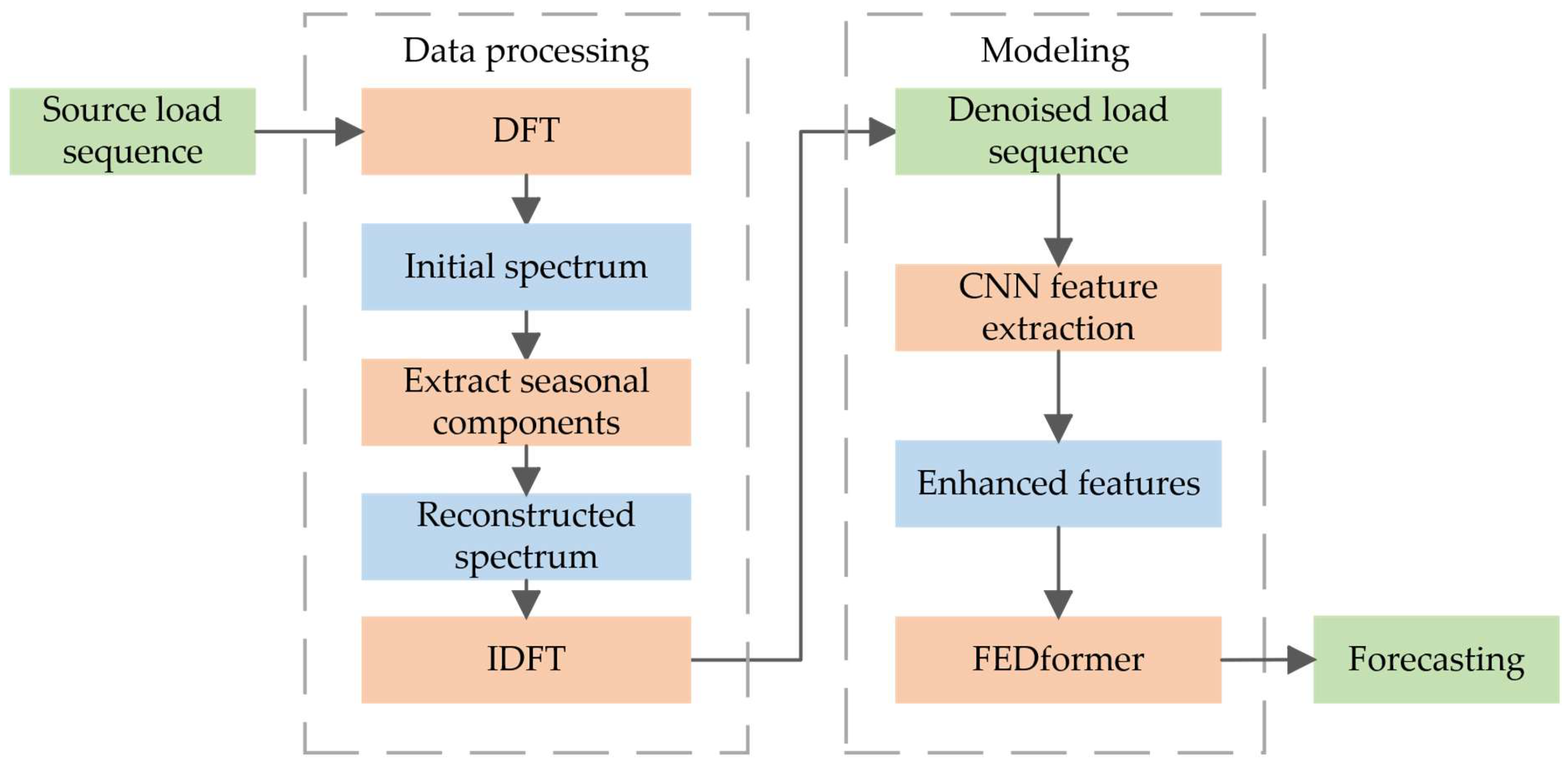
The brief process of the method is shown in Figure 1.

2.2. DFT Denoising Block

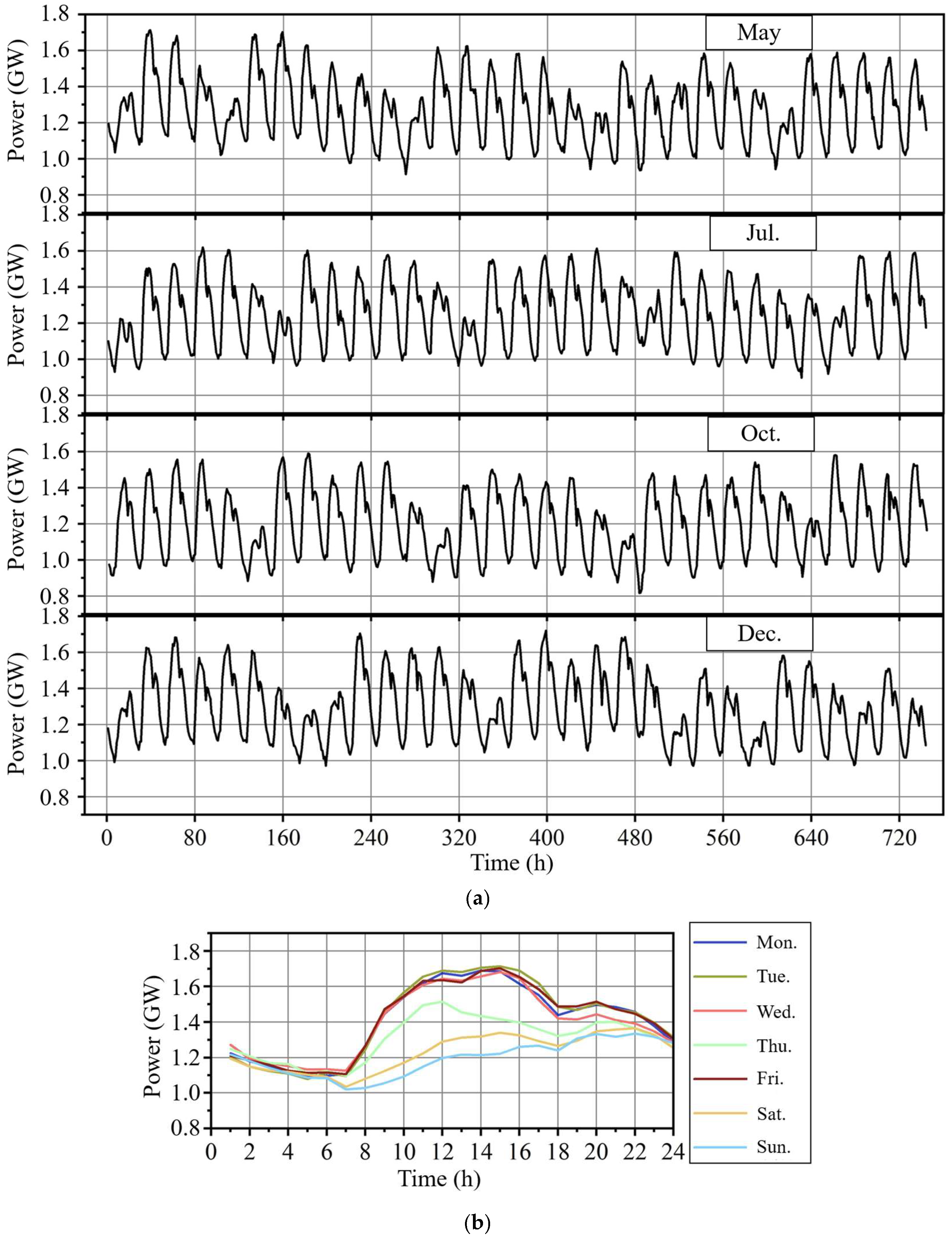
FEDformer is a general forecasting approach and performs random selection of frequency components. However, power load sequences normally contain high-frequency noise caused by occasional and sporadic events, such as acquisition errors, device faults, etc., which reduce the forecasting precision. Therefore, a data cleansing process that filters the high-frequency noise before FEDformer is required. Firstly, a DFT block is used to denoise electricity load sequences, to eliminate the influence of high frequency, and manual data cleansing is no longer required in our process. Daily and weekly periodic components (E_day, E_week) are extracted to improve the distinction of the characteristics of the data input. The reason why daily and weekly components are used is that the seasonality is strongly present in days and weeks, which is the natural characteristic of power load sequences. Then, the processed data is input into the CNN-FEDformer hybrid network structure, where CNN extracts local features from the data, constructs dense feature vectors, and reduces the input dimensionality of FEDformer. Figure 2 shows the seasonal characteristics of the load series. In Figure 2a, weekly and daily characteristics can be clearly observed in the load series of four months. In Figure 2b, daily characteristics of the 7 days in a week are displayed, illustrating that although the magnitudes of the load power are different in different days, the similarity of the variation trends is obvious. Therefore, Figure 2 proves that it is reasonable to extract daily and weekly periodic components by DFT.

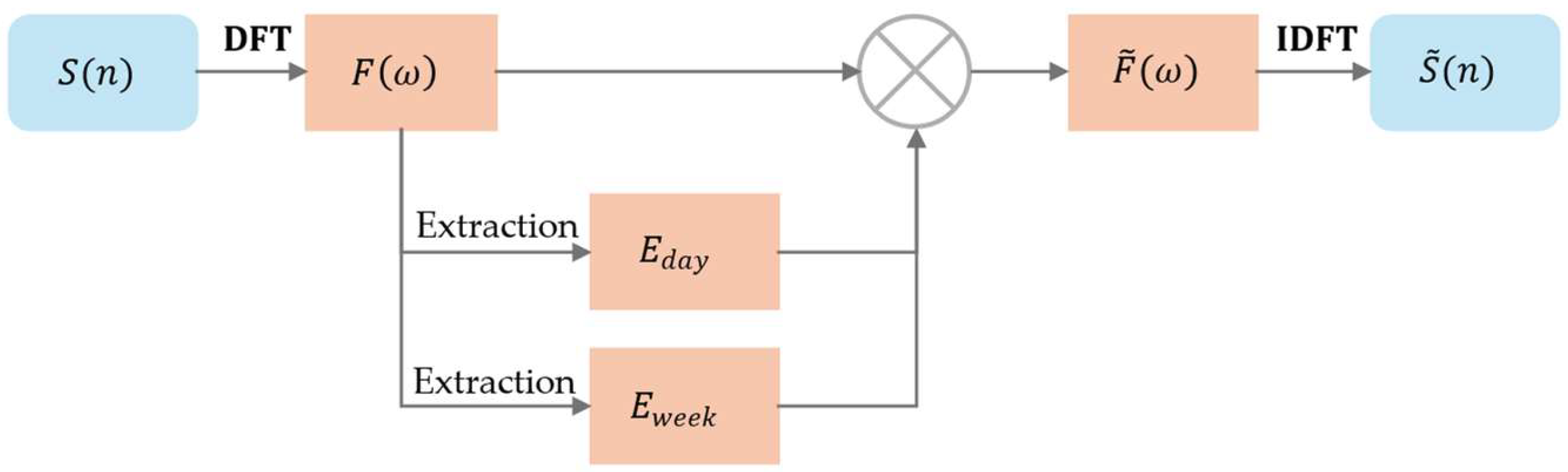
Low-frequency components in load time sequences contain valid features. High-frequency components reflect various irregular factors, manifesting as random fluctuations in the load. These high-frequency components represent the comprehensive variation characteristics caused by external, occasional, or sporadic events that occur randomly, which are the main sources of increasing forecasting errors. Therefore, it is necessary to segment and filter the high-frequency components. The DFT denoising block converts the input load sequence from the time domain to the frequency domain and extracts the daily and weekly periodic components from the spectrum. Periodic components play a crucial role in the development and trend of power load, with the daily and weekly components being the most prominent. Subsequently, the frequency signals are integrated to eliminate the interference of random abnormal factors, highlight the periodicity of the load sequence, and make the load data more stable. Finally, the denoised spectrum is projected back to the time domain through the inverse discrete Fourier transform. The structure of the data processing module is shown in Figure 3.

According to Figure 3, the DFT-based denoising process can be described as follows:

• Considering a time sequence $S\left(n\right)$, DFT is applied to the sequence to get the corresponding spectrum $F\left(\omega \right)$. For a forecasting purpose, a sequence used in training should be split into a historical sequence and a future sequence and processed separately.
• The spectral components whose corresponding frequency are the integer multiple of the daily sampling rate are selected as the daily components labeled by E_day.
• The spectral components whose corresponding frequency are the integer multiple of the weekly sampling rate are selected as the weekly components E_week.
• The selected daily and weekly components are integrated to form a new spectrum $\tilde{F}\left(\omega \right)$.
• The denoised time sequence $\tilde{S}(n)$ is achieved by an IDFT from $\tilde{F}\left(\omega \right)$

The DFT can be represented by Equation (1):

$$F\left(\omega \right)= \sum _{n=0}^{N-1}S(n)e^{-j\left(\frac{2\pi }{N}\right)n\omega }$$

(1)

where N is the length of the time sequence to be processed. DFT extracts daily and weekly periodic components in the frequency domain. Its global time-frequency transformation fully accounts for variations in load data across different time periods, offering strong interpretability. Daily and weekly periodic components exhibit the most noticeable periodic changes in the load data.

The quality of power load data significantly impacts the precision of load forecasting, thus imposing higher requirements on the data. By applying the DFT, the time-domain sequence is transformed into a frequency-domain sequence, from which daily and weekly periodic components are extracted. In the DFT spectrum $F\left(\omega \right)$, the realistic frequency $f_{\omega }$ is reflected by:

$$f_{\omega }={\displaystyle \frac{\omega }{T}} =\omega {\displaystyle \frac{f_s}{N}}=f_s/{\displaystyle \frac{\omega }{N}}$$

(2)

where $f_s$ is the sampling rate of a period, and $f_{\omega }$ must integer when the corresponding spectral component is periodic. Define daily sampling rate m (e.g., m = 96 when the sampling interval is 15 min), so that m × 7 is the weekly sampling rate. Equations (3) and (4) show the process that extracts the daily and weekly periodic components. $E_{day}$ and $E_{week}$ are the sets of subscripts of daily and weekly periodic components.:

$$E_{day}(\omega )=\left\{\begin{array}{ll}1,& mod\left(m,{\displaystyle \frac{M}{\omega }}\right)=0\\ 0,& other\end{array}\right.$$

(3)

$$E_{week}(\omega )=\left\{\begin{array}{ll}1,& mod\left(m\times 7,{\displaystyle \frac{M}{\omega }}\right)=0\\ 0,& other\end{array}\right.$$

(4)

where k represents the frequency subscript of the power load, and M is the length of the sequence. By integrating the components E_week and E_day, a denoised spectrum is formed by Equation (5):

$$\begin{gathered} \Omega \left(\omega \right)=E_{day}\left(\omega \right)\cup E_{week}\left(\omega \right) \\ \tilde{F}\left(\omega \right)= \Omega \left(\omega \right)·F\left(\omega \right) \end{gathered}$$

(5)

Finally, we use the Inverse Discrete Fourier Transform to convert the denoised spectrum $\tilde{F}\left(\omega \right)$ back into the time sequence, as shown in Equation (6). Denote $\tilde{S}\left(n\right)$ as the load of the denoised time sequence at time n, and $\tilde{F}\left(\omega \right)$ represents the integrated spectrum, which is the amplitude corresponding to frequency $\omega$.

$$\tilde{S}(n)={\displaystyle \frac{1}{N}} \sum _{\omega =0}^{N-1}F\left(\omega \right)e^{-j\left(\frac{2\pi }{N}\right)-n\omega }$$

(6)

2.3. Structure of the Load Forecasting Network

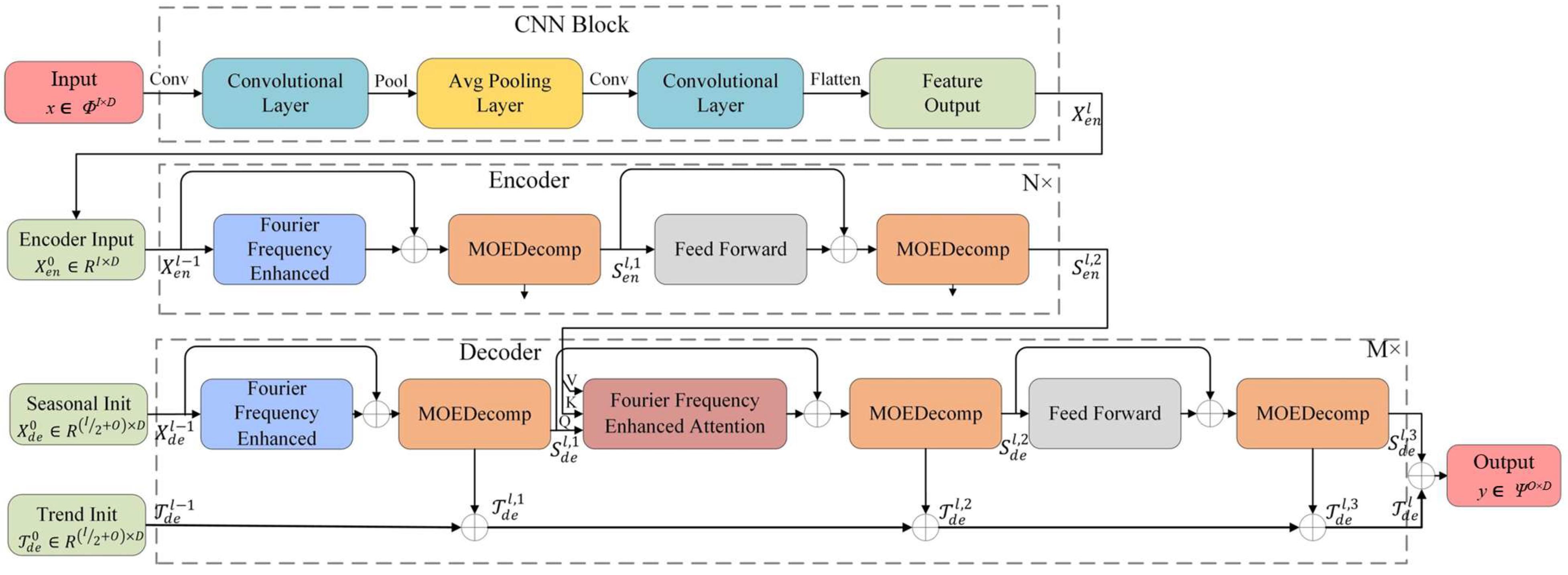
In this paper, we use CNN-FEDformer as the load forecasting module. The overall framework of the CNN-FEDformer method is composed of an encoder-decoder structure. Similar to the Transformer, the structure of the forecasting method is shown in Figure 4.

According to [38], in the FEDformer architecture, the frequency features are extracted and enhanced by the Fourier Frequency Enhanced block (FEB-f). Hence, the Fourier transformer and its inverse are performed in FEB-f. The Frequency Enhanced Attention mechanism (FEA-f) can identify dependency patterns in the frequency domain, guiding the method to focus on important features and revealing the contribution of different features to decision-making. This enables more efficient and accurate modeling of the global input-output relationships. A preceding CNN is added to the foundation of FEDformer to extract local features of the time series data, providing refined inputs for FEDformer. The input $x\in {\Phi }^{I\times D}$ denotes the sequences with an input length I and an input dimension D. The output $y\in {\Psi }^{O\times D}$ denotes the sequences with an output length O and an output dimension D.

2.3.1. Local Feature Extraction Using CNN

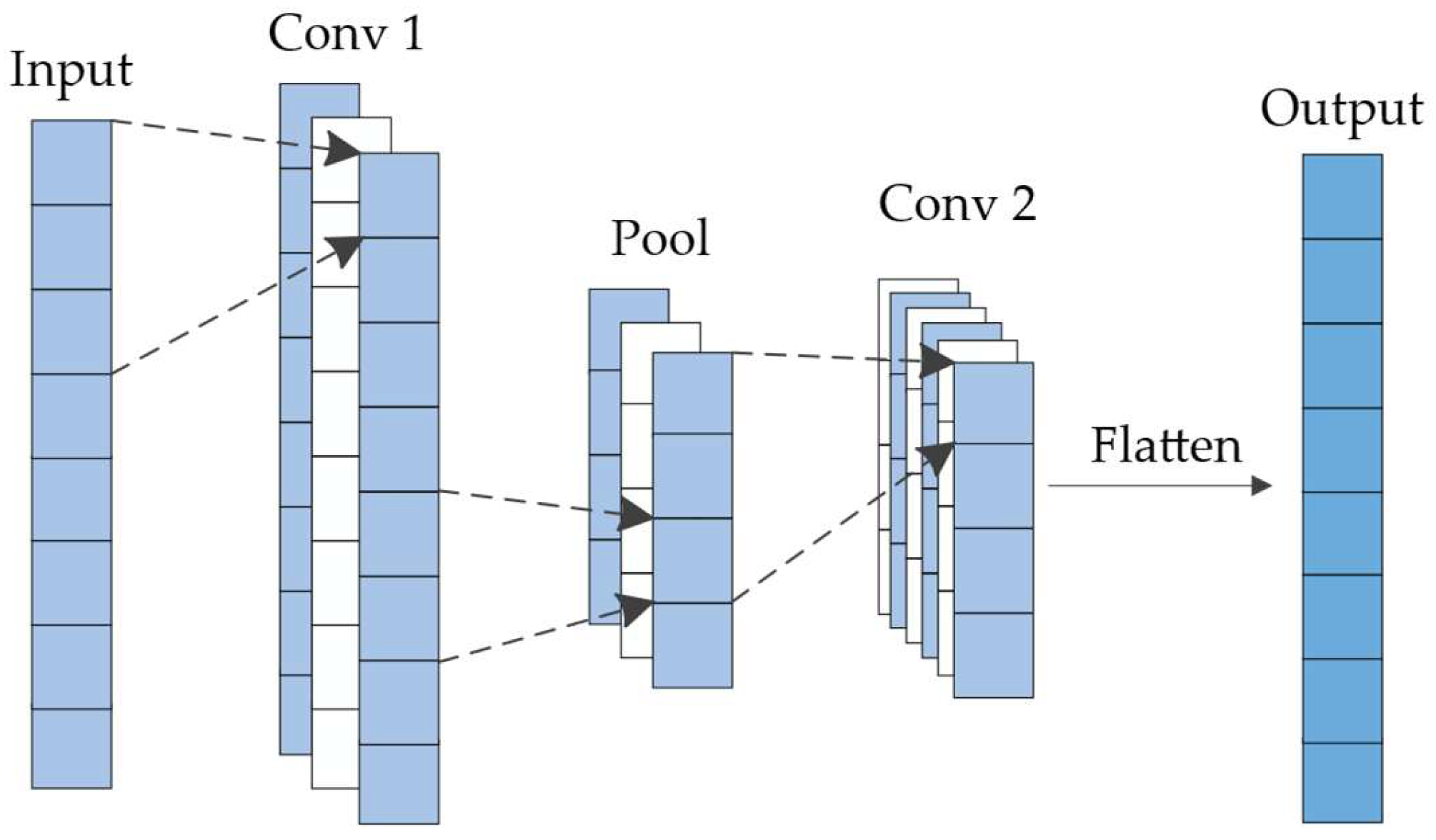
The local correlation of time series data is reflected in the continuous changes within a time slot, and convolutional filters can effectively capture the local features of the time series. Therefore, for the task of short-term load forecasting, this paper employs a CNN as the first encoding layer to capture local dependencies in the input sequence. The CNN structure is shown in Figure 5. The CNN uses local connectivity and shared weights, alternating between convolutional (conv) and pooling layers (pool) to obtain representations from raw sequence data, thereby capturing local feature information within the data.

The length and dimension of the input layer are equal to the FEDformer input size I × D, and the values are from the subsequences by applying an I-length sliding window to the DFT denoised sequence. The CNN consists of two convolutional layers and one pooling layer. Subsequently, a Flatten operation is applied to form sequences matching the size of FEDformer. The detailed architecture of the applied CNN for feature extraction is displayed in

Table 1. Architecture of the applied CNN.

Parameter	Parameter Value
Input length	96
Output length	96
Kernal size	3
Conv1 channels	32
Conv2 channels	64
Stride	1
Padding	Same
Pooling method	Average
Pooling size	2
Dropout rate	0.1
Nomalization	BatchNorm
Activation	GeLu

:

To reach an optimal architecture for feature extraction, deeper CNNs and a Temporal Convolutional Network (TCN) [40] are also applied. However, in the experiment, they do not show superior effectiveness; instead, they increase complexity. To balance effectiveness and efficiency, we finally select a simple architecture with two convolutional layers as the feature extractor.

2.3.2. Load Forecasting Using FEDformer

FEDformer [38] adopts an encoder-decoder architecture, where the encoder consists of a Frequency Enhanced Block with Fourier Transform (FEB-f), Mixture of Experts Decomposition (MOEDecomp), feed-forward block, and residual connection. The FEB-f helps reduce the method’s computational complexity based on the sparsity of time-series data in the frequency domain. MOEDecomp decomposes the sequence into seasonal and trend components. The feedforward neural network layers enhance the method’s ability to extract nonlinear features, and the residual connections effectively prevent gradient vanishing and model degradation issues. The Frequency Enhanced Attention with Fourier Transform (FEA-f) is performed in the decoder, where the encoder provides keys and values, and the decoder provides queries. Cross-attention is then applied after frequency domain enhancement.

The Encoder employs frequency domain feature extraction and decomposition to capture long-term dependencies in the sequential feature inputs. The load data is input into the FEB-f layer for time-frequency conversion, where a fixed number of high and low frequency components are randomly selected, and the selection mode is optimized during the training process to capture representative spectral features as well as to reduce computation complexity. The data is then converted back to the time domain for seasonal trend decomposition, and the decomposed seasonal components are further processed by a feedforward layer to enhance feature extraction and decomposition of the seasonal components. The decomposition process in the Encoder is described in Equation (7):

$$\left\{\begin{array}{c}{S}_{en}^l=MOEDecomp\left(FEB\left(X_{en}^{l-1}\right)+X_{en}^{l-1}\right)\\ S_{en}^{l‘}=MOEDecomp\left(FeedForward\left(S_{en}^l\right)+S_{en}^l\right)\\ S_{en}^{l‘}=X_{en}^l\end{array}\right.$$

(7)

where $S_{en}^l$ represents the seasonal component decomposed by the first block in the Encoder; $X_{en}^{l-1}$ represents the sequence data input to the Encoder, and $X_{en}^0$ represents the embedded historical sequence input.

Decomposition method: By fitting historical data, the time series is decomposed into various distinct feature components. The time series data enhanced by the frequency method (FEB-f) is decomposed by the decomposition module into trend and periodic components, as shown in Equation (8):

$$X\left(t\right)=X_{trend}+X_{seasonal}+{\epsilon }_i$$

(8)

where $X_{trend}$ represents the trend component, indicating the non-periodic change trend of the time series. $X_{seasonal}$ represents the seasonal component, typically referring to regular fluctuations on a daily, weekly, monthly, or annual basis. ${\epsilon }_i$ represents the residual, which refers to white noise in the data, with an expectation of 0.

The Decoder structure is similar to the encoder, with the seasonal and trend components superimposed and decomposed through multiple decomposition blocks. The key feature is the use of the FEA-f frequency-enhanced attention mechanism in the decoder to capture global dependencies in the frequency domain. In FEA-f, the Fourier transform is used to convert the input forms of the attention mechanism (queries, keys, values) from the time domain to the frequency domain. This is followed by the execution of the attention mechanism in the frequency domain by randomly selecting M patterns similar to FEB-f. The specific formulas are shown in Equations (9) and (10):

$$\left\{\begin{array}{c}\tilde{Q}=Select\left(F\left(q\right)\right)\\ \tilde{K}=Select\left(F\left(k\right)\right)\\ \tilde{V}=Select\left(F\left(v\right)\right)\end{array}\right.$$

(9)

$$FEA\left(q,k,v\right)=F^{-1}\left(Padding\left(tanh\left(\tilde{Q}·{\tilde{K}}^T\right)·\tilde{V}\right)\right)$$

(10)

where $q,k,v$ represent the queries, keys, and values in the Frequency-Enhanced Attention mechanism (FEA);$\tilde{K}, \tilde{V}$ are similar to $\tilde{Q}$ in FEB, all of which are randomly selected, and then the tanh activation function is used for the cross-attention mechanism.

3. Experiments and Results

This paper provides detailed information on the experimental configuration and conducts extensive experiments on two popular public datasets and one private dataset for validation.

To improve robustness and avoid the influence of randomness, for each method in our experiment, we vary the hyperparameters, run 10 rounds with random seeds and the same hyperparameters, compute the mean of the results of every 10 rounds, and select the best mean MAE to determine the hyperparameters for the method. Therefore, the results presented below are the best mean value of the MAE achieved by each method.

3.1. Configurations of the Experiments

3.1.1. Datasets for the Experiments

The datasets utilized in the paper involve monitoring data from power apparatuses and distributed grids, to prove the generalization capability of the proposed method. Two public datasets, as well as a private dataset, are applied, as summarized in

Table 2. Details of the datasets.

Dataset	Num. of Examples	Num. of Dims	Sampling Frequency
ETTm2	69,680	8	15 min
ECL	26,304	321	1 h
ELTS	48,000	13	1 h

:

• Transformer Oil Temperature (ETT) dataset [39]: a public dataset comprises multiple versions collected from two power stations at different sampling intervals (15 min and 1 h). This paper uses the ETTm2 dataset, which has a sampling frequency of 15 min, for experiments. The dataset contains multiple load columns and an oil temperature column, with a total of 69,680 sampling points.
• Electricity Consuming Load (ECL) dataset [41]: a public dataset includes power consumption data from multiple users within a region. It contains 321 user instances, each of which represents the electricity consumption of a user over three years.
• Electric Load Time Sequences (ELTS) dataset: a private dataset contains power load data collected by our collaborative company from a specific region between 2015 and 2020 (sampled at 1-h intervals, 24 points per day). This comprehensive dataset has 13 columns related to our research, including the power load, temperature, wind speed, relative humidity, and liquid precipitation from Panama City, Santiago City, and David City. There are a total of 48,000 sampling points.

Each dataset is applied to train a model. The data pipeline is formed as follows:

• Fragments that have significant errors, e.g., multiple abnormal values in a row, are removed manually.
• The values in each dimension are normalized into [0, 1] respectively.
• The dataset is divided into training, validation, and test sets in a 7:1:2 ratio.
• During the training process, to avoid data leakage, historical sequences before the prediction time and future sequences after the prediction time are denoised by the DFT block separately.
• During the testing process, to make a fair comparison with other methods, only input sequences are denoised, and forecasting errors are computed between predicted and initial sequences.

3.1.2. Evaluation Metrics

The FEDformer model in this paper is trained using the hyperparameters that achieve the optimal precision, as shown in

Table 3. Configuration of FEDformer.

Parameter	Tuned	Parameter Value
Input length	No	96
Prediction length	No	12, 24, 96
Num. of encoder layers	No	2
Num. of decoder layers	No	1
Attention heads	Yes	8
Dimension of model	Yes	1024
Dimension of fcn	Yes	2048
Activation	No	GeLu
Dropout rate	Yes	0.1

. The ‘Tuned’ column indicates whether the hyperparameter is constant or tuned in the experiment. The hyperparameters of other methods for comparison are tuned in the same way to achieve the best precision. In the following experiments, the results are achieved by using a forecasting sequence length of 96 samples. However, sequence lengths of 12 and 24 samples are also inspected in our experiments. The Mean Square Error (MSE) is used for loss computation, and the Mean Absolute Error (MAE) is used to evaluate the precision in tests.

The configuration of training is presented in

Table 4. Training configuration.

Parameter	Parameter Value
Optimizer	Adam
Learning rate	0.0001
Loss	MSE
Epochs	30
Batch size	32
Early stopping	Loss ≤ 0.001

.

We train and test the model on a workstation with an Intel Core i9-10900X CPU and a NVDIA RTX 2080 Ti GPU, as well as Pytorch 2.4.0. The seeds are randomly generated as most researchers commonly do.

3.2. Results of Load Sequence Denoising

The load data is input into the DFT block for denoising. As described in Section 2.2 and Equations (1) and (2), the key to the DFT decomposition block lies in determining the frequency domain decomposition scale. This paper selects daily and weekly cycle components as the frequency-domain decomposition scales, because the main components forming the power load trends are the daily and weekly cycles, followed by mid- to low-frequency components that are highly sensitive to related factors.

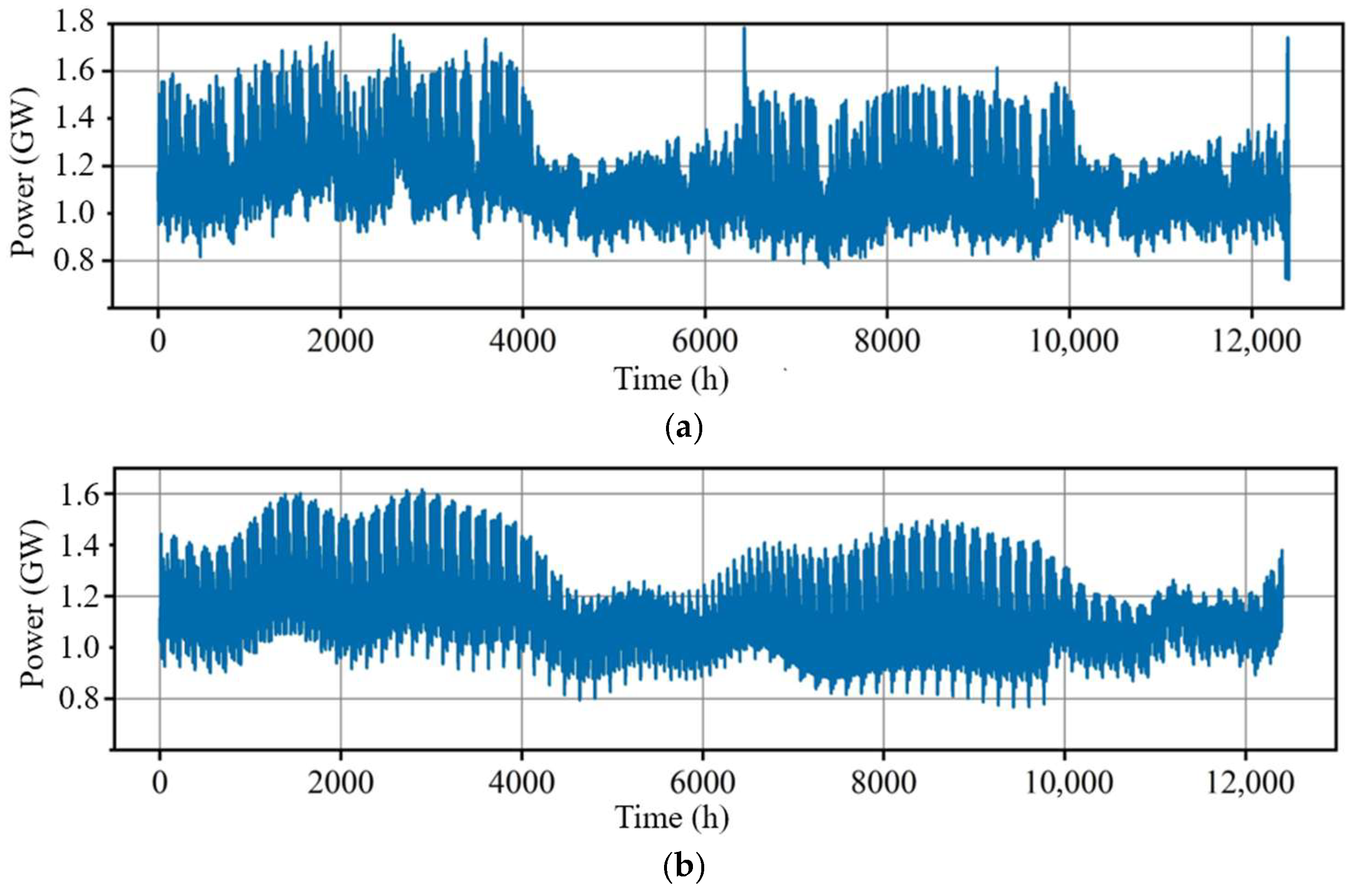
By using Equation (3) to perform spectrum superposition, the periodic components with obvious electricity usage characteristics are superimposed to obtain the denoised spectrum. Subsequently, the Inverse Discrete Fourier Transform (IDFT) is applied to restore the denoised spectrum to the time sequence, as shown in Figure 6.

Comparing Figure 6a,b, the abnormal fluctuations in the sequence are significantly cancelled by DFT. Therefore, DFT denoising is applied in the following experiments. After reconstruction, the forecasting precision can be improved. In the subsequent experiments, we will verify the effectiveness of DFT in improving model performance. To verify the effectiveness of the denoising process, we perform outlier detection [42] to compare the sequences before and after denoising. We apply the z-score as the detection method and vary the threshold. The moving window length is the number of samples per week.

Table 5. Outlier analysis.

Dataset	z-Score Threshold = 3		z-Score Threshold = 2
	Before	After	Before	After
ETTm2	0.03%	0.00%	0.81%	0.01%
ECL	0.02%	0.00%	0.84%	0.00%
ELTS	0.02%	0.00%	0.56%	0.00%

shows the percentage of outlier points before and after denoising.

3.3. Ablation Experiments and Comparisons

To further verify the contributions of each block within the overall model framework, the influence on model performance is assessed by gradually removing components from the model framework. Specifically, three experimental groups are designed: the first group conducts ablation experiments on the baseline methods with the data denoising block; the second group conducts ablation experiments on the baseline methods with the convolutional neural network (CNN), and the third group compares the baseline methods with both the data denoising block and the CNN.

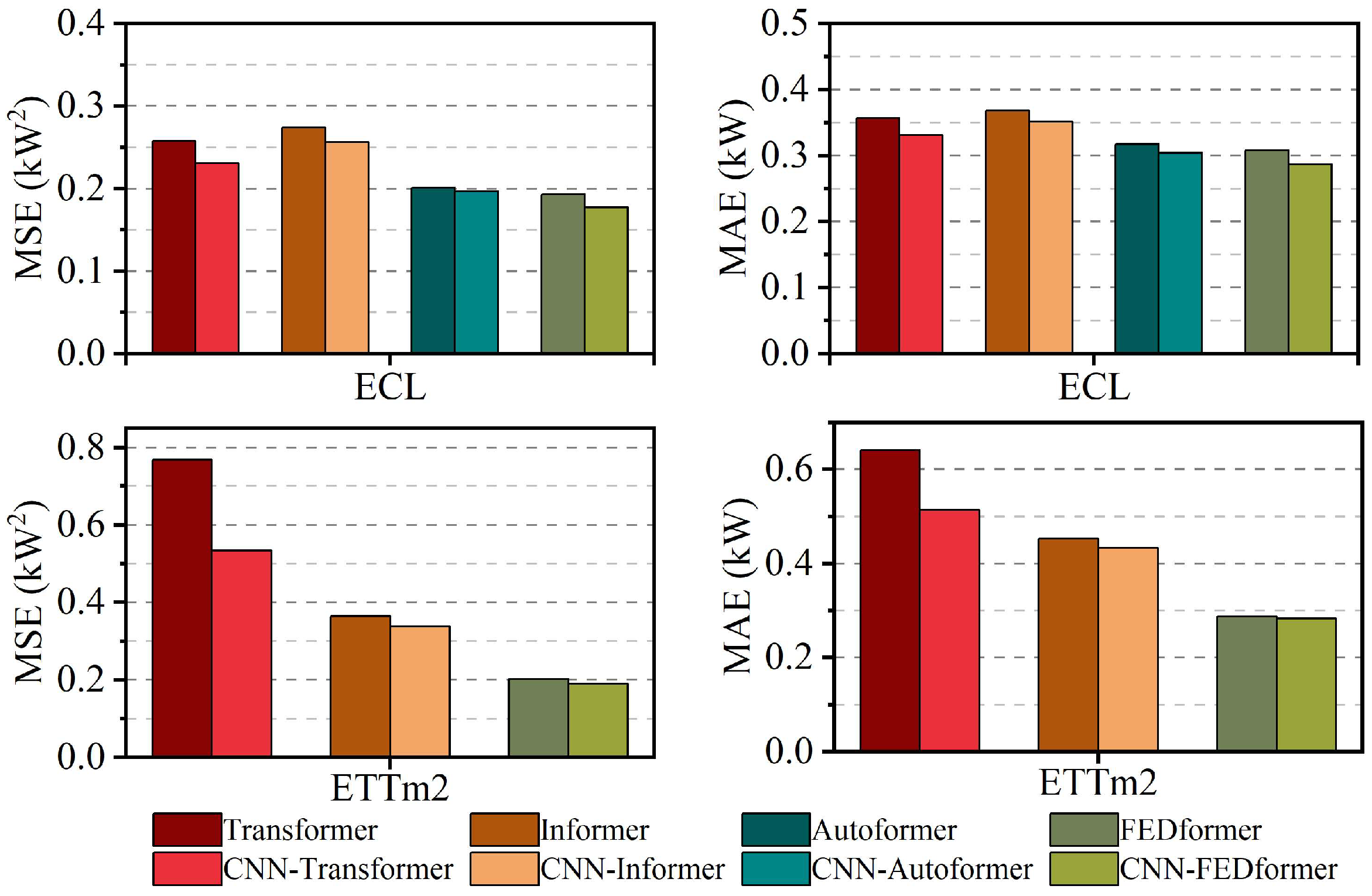
With the ECL dataset, the MSEs and MAEs of CNN-Transformer (C-Transformer), CNN-Informer (C-Informer), CNN-Autoformer (C-Autoformer), and CNN-FEDformer (C-FEDformer) are all reduced compared to the baseline methods. With the ETTm2 dataset, the methods CNN-Transformer, CNN-Informer, and CNN-FEDformer are validated, and the results show that the MSE and MAE of the three methods are reduced to varying degrees, as shown in

Table 6. Results of the ablation experiment.

Type	Method	MSE		MAE
		ECL	ETTm2	ECL	ETTm2
BASE	LSTM	0.375	2.041	0.437	1.073
	Transformer	0.258	0.768	0.357	0.642
	Informer	0.274	0.365	0.368	0.453
	Autoformer	0.201	0.255	0.317	0.339
	FEDformer	0.193	0.203	0.308	0.287
DFT	D-LSTM	0.348	1.877	0.411	1.021
	D-Transformer	0.240	0.698	0.338	0.587
	D-FEDformer	0.172	0.185	0.284	0.265
CNN	C-Transformer	0.247	0.533	0.341	0.513
	C-Informer	0.256	0.338	0.351	0.433
	C-Autoformer	0.197	/	0.304	/
	C-FEDformer	0.177	0.189	0.287	0.283
TCN	T-Transformer	0.273	0.492	0.321	0.505
	T-Informer	0.245	0.343	0.480	0.444
	T-FEDformer	0.209	0.182	0.259	0.305

. By comparing various metrics, the improved forecasting methods in this paper achieve the best results on the two public datasets, validating the effectiveness of CNN in enhancing forecasting precision. We also apply a Temporal Convolutional Network (TCN) [40] for comparison (T-Transformer, T-Informer, T-FEDformer). It can be noticed that some of the combinations, such as D-Informer, D-Autoformer, T-Autoformer, etc., are missing in Table 6 because the training processes fail as forecasting errors do not effectively decline.

3.3.1. Ablation Experiment for DFT

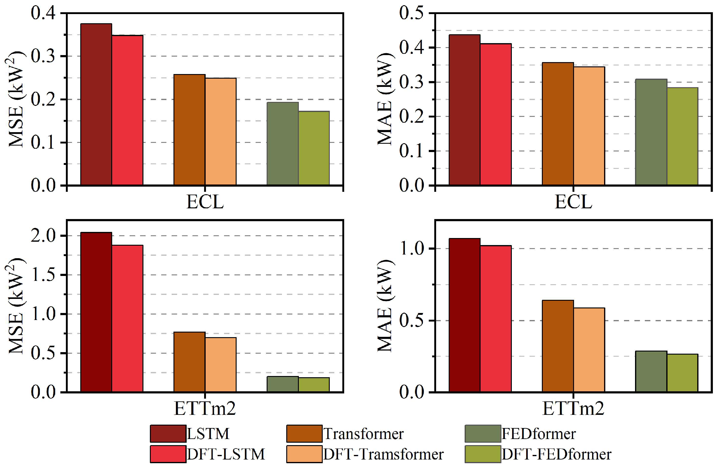
To validate the effectiveness of DFT in enhancing the precision of forecasting after denoising the time sequence, the validation focuses on the public datasets ECL and ETTm2. The experiment compares two schemes: with and without DFT denoising. Load forecasting is performed using LSTM, Transformer, and FEDformer, with the results shown in Figure 7.

It can be seen from the figure that after denoising the input data with DFT, the model performance is superior to the original methods. Specifically, with the ECL dataset, the MSEs of DFT-LSTM (D-LSTM), DFT-Transformer (D-Transformer), and DFT-FEDformer (D-FEDformer) decrease by 0.027, 0.018, and 0.021, respectively, compared to the original methods; the MAEs decrease by 0.026, 0.019, and 0.024, respectively. With the ETTm2 dataset, the MSEs of the DFT-LSTM, DFT-Transformer, and DFT-FEDformer decrease by 0.164, 0.07, and 0.018, respectively, compared to the original methods; the MAEs decrease by 0.052, 0.055, and 0.022, respectively. By comparing the MSEs and MAEs, the results of the three methods with DFT denoising are all superior to those of the original. This validates the effectiveness of DFT denoising.

3.3.2. Ablation Experiment for CNN

To explore the effectiveness of the composite forecasting model mentioned in this paper, multiple different composite models are validated on the same dataset. Using the ablation approach, the baseline methods selected are Transformer, Informer, Autoformer, and FEDformer, and their performance is compared with their CNN-combined versions to validate error reduction, as shown in Figure 8.

Finally, considering the result shows that the more complex TCN does not significantly improve precision. Therefore, the proposed CNN architecture is selected for higher efficiency.

3.3.3. Comparisons of the Final Results

To further validate the advantages of the forecasting method proposed in this paper, we conduct comparative experiments with commonly used methods in the load forecasting field, including Long Short-Term Memory (LSTM), Transformer, Informer, Autoformer, and FEDformer. In particular, LSTM and Transformer are combined with the method proposed in this paper for a deeper comparison with the improved model, named DCL and DCTformer, respectively. Nevertheless, other hybrid patterns, such as DFT + CNN + Autoformer/Informer, cannot be successfully trained with our datasets during the experiment. In order to make a fair comparison, we have tuned the hyperparameters of the methods to achieve the best precision. The experimental results, as shown in

Table 7. Comparison between different forecasting methods.

Method	Metric	ECL			ETTm2			ELTS
		12	24	96	12	24	96	12	24	96
DCFformer	MSE	0.147	0.152	0.167	0.092	0.103	0.179	0.0101	0.0106	0.0132
	MAE	0.256	0.268	0.274	0.197	0.218	0.263	0.0188	0.0221	0.0247
	MAPE	1.75%	1.89%	1.86%	1.29%	1.40%	1.69%	0.99%	1.21%	1.32%
	STD	0.045%	0.056%	0.061%	0.040%	0.045%	0.049%	0.027%	0.043%	0.035%
DCTformer	MSE	0.209	0.221	0.239	0.302	0.329	0.696	0.0256	0.0308	0.0386
	MAE	0.312	0.317	0.338	0.433	0.446	0.582	0.0315	0.0389	0.0452
	MAPE	2.17%	2.18%	2.37%	2.84%	2.91%	3.72%	1.71%	2.08%	2.51%
	STD	0.063%	0.055%	0.055%	0.072%	0.091%	0.097%	0.047%	0.054%	0.070%
DCL	MSE	0.308	0.312	0.342	1.039	1.222	1.852	0.0349	0.0396	0.0461
	MAE	0.407	0.414	0.401	0.937	0.941	1.018	0.0369	0.0401	0.0418
	MAPE	2.81%	2.81%	2.84%	6.16%	6.26%	6.58%	2.03%	2.21%	2.28%
	STD	0.089%	0.076%	0.038%	0.205%	0.190%	0.208%	0.046%	0.074%	0.058%
FEDformer	MSE	0.154	0.161	0.193	0.096	0.114	0.203	0.0111	0.0116	0.0155
	MAE	0.287	0.281	0.308	0.205	0.224	0.287	0.0189	0.0232	0.0263
	MAPE	1.96%	1.96%	2.20%	1.32%	1.43%	1.85%	1.01%	1.29%	1.43%
	STD	0.056%	0.056%	0.067%	0.032%	0.037%	0.061%	0.035%	0.044%	0.037%
Autoformer	MSE	0.185	0.189	0.201	0.101	0.132	0.255	0.0153	0.0157	0.0189
	MAE	0.309	0.312	0.317	0.142	0.279	0.339	0.0276	0.0283	0.0302
	MAPE	2.11%	2.15%	2.16%	0.93%	1.78%	2.16%	1.49%	1.56%	1.61%
	STD	0.050%	0.061%	0.071%	0.026%	0.055%	0.056%	0.044%	0.039%	0.036%
Informer	MSE	0.229	0.233	0.274	0.125	0.276	0.369	0.0631	0.0659	0.0712
	MAE	0.349	0.357	0.368	0.252	0.399	0.453	0.0582	0.0597	0.0643
	MAPE	2.39%	2.54%	2.56%	1.61%	2.57%	2.93%	3.16%	3.23%	3.41%
	STD	0.072%	0.057%	0.074%	0.051%	0.081%	0.068%	0.102%	0.110%	0.080%
Transformer	MSE	0.217	0.231	0.258	0.106	0.152	0.768	0.0356	0.0398	0.0475
	MAE	0.330	0.339	0.357	0.225	0.280	0.642	0.0438	0.0472	0.0541
	MAPE	2.32%	2.41%	2.50%	1.43%	1.86%	4.09%	2.32%	2.53%	2.89%
	STD	0.056%	0.080%	0.068%	0.042%	0.042%	0.114%	0.065%	0.058%	0.071%
LSTM	MSE	0.311	0.314	0.375	1.239	1.320	2.041	0.0451	0.0500	0.0524
	MAE	0.415	0.419	0.437	0.921	0.961	1.073	0.0517	0.0539	0.0557
	MAPE	2.88%	2.90%	3.07%	6.13%	6.21%	7.02%	2.80%	2.96%	3.07%
	STD	0.055%	0.096%	0.100%	0.184%	0.172%	0.150%	0.057%	0.060%	0.098%

Note: the units of MSE and MAE of ECL and ETTm2 are kW and kW², while those for ELTS are GW and GW².

, provide a comprehensive comparison across three datasets. Since the units of the datasets are different, we also apply MAPE as a metric. The standard deviation of the MAPEs (the STD rows) of every 10 rounds is shown to verify robustness. Compared to the existing methods, our improved method proposed in this paper not only excels in individual metrics but also demonstrates superior overall performance. On the other hand, the method proposed in this paper also improves the performance of other baseline methods when applied to them, which is well demonstrated by LSTM and Transformer.

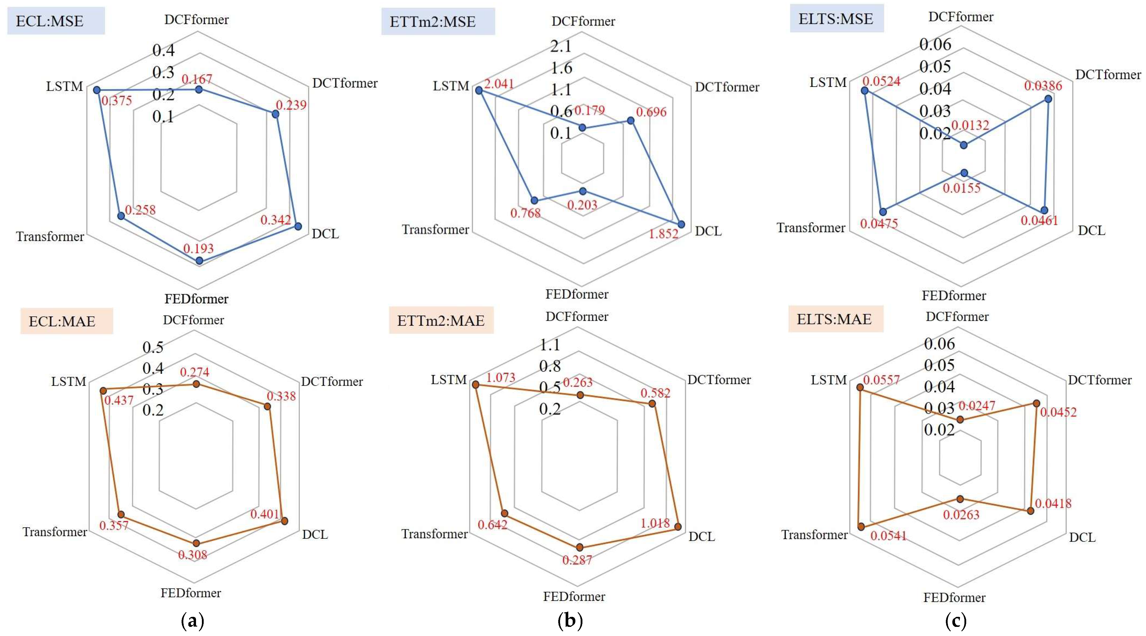
To further demonstrate the effectiveness of the proposed method, as shown in Figure 9, in addition to DCFformer, LSTM, and Transformer are also combined to compare.

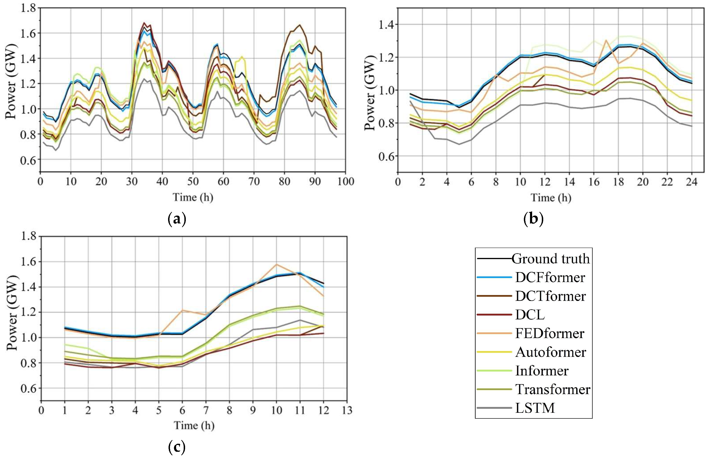
Different datasets have a great impact on the forecasting precision because of the different loads and indicators. It can be clearly observed that the proposed DCFformer achieves the best forecasting precision under the three datasets and two evaluation metrics. After incorporating the data denoising and local feature extraction blocks, the forecasting precision of LSTM and Transformer is also significantly improved, which verifies the effectiveness and generalization of the proposed method for enhancing forecasting performance. To explain the precision of each method more intuitively, we select the ELTS dataset and respectively choose forecasting lengths of 96, 24, and 12 from its test set. The forecasting results of each method are compared, as shown in Figure 10. In Figure 10a, the forecasting of DCFformer is closest to the ground truth. The precision of FEDformer is relatively lower than that of the proposed method, and its forecasting curve lacks smoothness, exhibiting minor fluctuations. In Figure 10b,c, in the 24 and 12 length cases, it is clearly observed that the forecast curve of FEDformer displays significant local fluctuations, which are attributed to the influence of outliers in the data, adversely affecting the precision of its forecasts. The forecasting results of LSTM and Transformer exhibit a significant deviation from the ground truth. However, when they are combined with the method proposed in this paper, i.e., DFT-CNN-LSTM (DCL) and DFT-CNN-Transformer (DCTformer), significant performance improvement is achieved, and the gap between the forecasting results and ground truth becomes smaller. Other Transformer-based approaches, i.e., Autoformer and Informer, perform lower precisions than our improved methods. Therefore, the proposed method can effectively learn local features of the power load data and grasp global dependencies, ultimately achieving accurate results.

3.3.4. Comparison of Memory and Computational Costs

We also compared the memory and computational costs utilized by the methods described above. Considering LSTM is in a different category and reaches significantly lower forecasting precision, it is not discussed in this section. The counts of the parameters that directly reflect the memory cost are shown in

Table 8. Counts of parameters of different forecasting methods.

Method	Parameter Count per Layer (Million)
	12	24	96
DCFformer	0.13	0.26	1.02
FEDformer	0.13	0.25	1.00
Autoformer	2.0	5.2	28.6
Informer	1.9	4.9	27.5
Transformer	5.8	21.4	314

.

Table 9. Computational efficiency of different forecasting methods.

Method	Training Time per Epoch (s)			Forecasting Time (ms)
	12	24	96	12	24	96
DCFformer	4	8	30	80	82	91
FEDformer	4	7	30	76	77	87
Autoformer	13	23	133	88	96	112
Informer	11	22	125	87	90	107
Transformer	27	85	396	99	185	766

shows the computational efficiency of the methods by comparing their training and prediction times on the same hardware.

Table 8 and Table 9 indicate that the proposed DCFformer requires equivalent memory and computing power as those of FEDformer, and significantly lower than those of Autoformer, Informer, and Transformer.

4. Conclusions and Further Work

This paper proposes the DCFformer for short-term load forecasting tasks. It uses DFT to eliminate interference of abnormal values from power load sequences; a CNN is employed to extract local features; and finally, in the frequency domain, it captures global dependencies with FEDformer. The experiments prove that, for power load forecasting, the proposed hybrid method is superior to existing methods, such as LSTM, Informer, and Autoformer.

There are several studies to be accomplished in future work:

• Denoising methods that extract components from load sequences with higher effectiveness and efficiency are to be investigated. For example, improved DWT is to be studied to suppress complex, multi-scale noise.
• Optimized network architecture and training mechanisms that improve forecasting precision and computational efficiency are to be investigated.
• The proposed methodology is expected to be implemented in practical applications such as distributed power networks, microgrids, etc. Modeling with realistic power data is required.
• The proposed model is expected to be optimized for the distribution to edge devices such as microgrid controllers, photovoltaic inverters, power distribution gateways, etc. A system framework containing both hardware and software is to be developed.

References

1. Kim, N.; Park, H.; Lee, J.; Choi, J.K. Short-Term Electrical Load Forecasting With Multidimensional Feature Extraction. IEEE Trans. Smart Grid 2022, 13, 2999–3013. [Google Scholar] [CrossRef]
2. Lin, W.; Wu, D.; Boulet, B. Spatial-Temporal Residential Short-Term Load Forecasting via Graph Neural Networks. IEEE Trans. Smart Grid 2021, 12, 5373–5384. [Google Scholar] [CrossRef]
3. Wang, Y.; Chen, J.; Chen, X.; Zeng, X.; Kong, Y.; Sun, S.; Guo, Y.; Liu, Y. Short-Term Load Forecasting for Industrial Customers Based on TCN-LightGBM. IEEE Trans. Power Syst. 2021, 36, 1984–1997. [Google Scholar] [CrossRef]
4. Dong, J.; Luo, L.; Lu, Y.; Zhang, Q. A Parallel Short-Term Power Load Forecasting Method Considering High-Level Elastic Loads. IEEE Trans. Instrum. Meas. 2023, 72, 2524210. [Google Scholar] [CrossRef]
5. Jiang, B.; Liu, Y.; Geng, H.; Wang, Y.; Zeng, H.; Ding, J. A Holistic Feature Selection Method for Enhanced Short-Term Load Forecasting of Power System. IEEE Trans. Instrum. Meas. 2023, 72, 2500911. [Google Scholar] [CrossRef]
6. Zhang, Z.; Liu, J.; Pang, S.; Shi, M.; Goh, H.H.; Zhang, Y.; Zhang, D. General Short-Term Load Forecasting Based on Multi-Task Temporal Convolutional Network in COVID-19. Int. J. Electr. Power Energy Syst. 2023, 147, 108811. [Google Scholar] [CrossRef]
7. Tarmanini, C.; Sarma, N.; Gezegin, C.; Ozgonenel, O. Short Term Load Forecasting Based on Arima and Ann Approaches. Energy Rep. 2023, 9, 550–557. [Google Scholar] [CrossRef]
8. Zhang, S.; Chen, R.; Cao, J.; Tan, J. A CNN and LSTM-Based Multi-Task Learning Architecture for Short and Medium-Term Electricity Load Forecasting. Electr. Power Syst. Res. 2023, 222, 109507. [Google Scholar] [CrossRef]
9. Saber, A.Y.; Alam, A.K.M.R. Short Term Load Forecasting Using Multiple Linear Regression for Big Data. In Proceedings of the 2017 IEEE Symposium Series on Computational Intelligence (SSCI), Honolulu, HI, USA, 27 November–1 December 2017; pp. 1–6. [Google Scholar]
10. Rendon-Sanchez, J.F.; de Menezes, L.M. Structural Combination of Seasonal Exponential Smoothing Forecasts Applied to Load Forecasting. Eur. J. Oper. Res. 2019, 275, 916–924. [Google Scholar] [CrossRef]
11. Jin, M.; Zhou, X.; Zhang, Z.M.; Tentzeris, M.M. Short-Term Power Load Forecasting Using Grey Correlation Contest Modeling. Expert Syst. Appl. 2012, 39, 773–779. [Google Scholar] [CrossRef]
12. Pooniwala, N.; Sutar, R. Forecasting Short-Term Electric Load with a Hybrid of ARIMA Model and LSTM Network. In Proceedings of the 2021 International Conference on Computer Communication and Informatics (ICCCI), Coimbatore, India, 27–29 January 2021; pp. 1–6. [Google Scholar]
13. Barak, S.; Sadegh, S.S. Forecasting Energy Consumption Using Ensemble Arima–Anfis Hybrid Algorithm. Int. J. Electr. Power Energy Syst. 2016, 82, 92–104. [Google Scholar] [CrossRef]
14. Medina Macaira, P.; Castro Sousa, R.; Cyrino Oliveira, F.L. Forecasting Brazil’s Electricity Consumption with Pegels Exponential Smoothing Techniques. IEEE Lat. Am. Trans. 2016, 14, 1252–1258. [Google Scholar] [CrossRef]
15. Wang, J.; Wang, J.; Li, Y.; Zhu, S.; Zhao, J. Techniques of Applying Wavelet De-Noising into a Combined Model for Short-Term Load Forecasting. Int. J. Electr. Power Energy Syst. 2014, 62, 816–824. [Google Scholar] [CrossRef]
16. Wu, K.; Wu, J.; Feng, L.; Yang, B.; Liang, R.; Yang, S.; Zhao, R. An Attention-Based Cnn-Lstm-Bilstm Model for Short-Term Electric Load Forecasting in Integrated Energy System. Int. Trans. Electr. Energy Syst. 2020, 31, e12637. [Google Scholar] [CrossRef]
17. Yang, Y.; Zhou, H.; Wu, J.; Liu, C.-J.; Wang, Y.-G. A Novel Decompose-Cluster-Feedback Algorithm for Load Forecasting with Hierarchical Structure. Int. J. Electr. Power Energy Syst. 2022, 142, 108249. [Google Scholar] [CrossRef]
18. Lin, X.; Zamora, R.; Baguley, C.A.; Srivastava, A.K. A Hybrid Short-Term Load Forecasting Approach for Individual Residential Customer. IEEE Trans. Power Deliv. 2023, 38, 26–37. [Google Scholar] [CrossRef]
19. Fan, G.-F.; Zhang, L.-Z.; Yu, M.; Hong, W.-C.; Dong, S.-Q. Applications of Random Forest in Multivariable Response Surface for Short-Term Load Forecasting. Int. J. Electr. Power Energy Syst. 2022, 139, 108073. [Google Scholar] [CrossRef]
20. Yin, L.; Sun, Z.; Gao, F.; Liu, H. Deep Forest Regression for Short-Term Load Forecasting of Power Systems. IEEE Access 2020, 8, 49090–49099. [Google Scholar] [CrossRef]
21. Mubashar, R.; Awan, M.; Ahsan, M.; Yasin, A.; Singh, V. Efficient Residential Load Forecasting Using Deep Learning Approach. Int. J. Comput. Appl. Technol. 2022, 68, 205–214. [Google Scholar] [CrossRef]
22. Yang, Y.; Che, J.; Deng, C.; Li, L. Sequential Grid Approach Based Support Vector Regression for Short-Term Electric Load Forecasting. Appl. Energy 2019, 238, 1010–1021. [Google Scholar] [CrossRef]
23. Ozcanli, A.K.; Yaprakdal, F.; Baysal, M. Deep Learning Methods and Applications for Electrical Power Systems: A Comprehensive Review. Int. J. Energy Res. 2020, 44, 7136–7157. [Google Scholar] [CrossRef]
24. Koprinska, I.; Wu, D.; Wang, Z. Convolutional Neural Networks for Energy Time Series Forecasting. In Proceedings of the 2018 International Joint Conference on Neural Networks (IJCNN), Rio de Janeiro, Brazil, 8–13 July 2018; pp. 1–8. [Google Scholar]
25. Shabbir, N.; Amadiahangar, R.; Raja, H.A.; Kütt, L.; Rosin, A. Residential Load Forecasting Using Recurrent Neural Networks. In Proceedings of the 2020 IEEE 14th International Conference on Compatibility, Power Electronics and Power Engineering (CPE-POWERENG), Setubal, Portugal, 8–10 July 2020; Volume 1, pp. 478–481. [Google Scholar]
26. Yuvaraju, M.; Divya, M. Residential Load Forecasting by Recurrent Neural Network on LSTM Model. In Proceedings of the 2020 4th International Conference on Intelligent Computing and Control Systems (ICICCS), Madurai, India, 13–15 May 2020; pp. 395–400. [Google Scholar]
27. Kong, W.; Dong, Z.Y.; Jia, Y.; Hill, D.J.; Xu, Y.; Zhang, Y. Short-Term Residential Load Forecasting Based on LSTM Recurrent Neural Network. IEEE Trans. Smart Grid 2019, 10, 841–851. [Google Scholar] [CrossRef]
28. Yamasaki, M.; Freire, R.Z.; Seman, L.O.; Stefenon, S.F.; Mariani, V.C.; dos Santos Coelho, L. Optimized Hybrid Ensemble Learning Approaches Applied to Very Short-Term Load Forecasting. Int. J. Electr. Power Energy Syst. 2024, 155, 109579. [Google Scholar] [CrossRef]
29. Rafi, S.H.; Masood, N.A.; Deeba, S.R.; Hossain, E. A Short-Term Load Forecasting Method Using Integrated CNN and LSTM Network. IEEE Access 2021, 9, 32436–32448. [Google Scholar] [CrossRef]
30. Chiu, M.-C.; Hsu, H.-W.; Chen, K.-S.; Wen, C.-Y. A Hybrid CNN-GRU Based Probabilistic Model for Load Forecasting from Individual Household to Commercial Building. Energy Rep. 2023, 9, 94–105. [Google Scholar] [CrossRef]
31. Vaswani, A.; Shazeer, N.; Parmar, N.; Uszkoreit, J.; Jones, L.; Gomez, A.N.; Kaiser, Ł.; Polosukhin, I. Attention Is All You Need. In Proceedings of the 31st International Conference on Neural Information Processing Systems, Long Beach, CA, USA, 4–9 December 2017; Curran Associates Inc.: Red Hook, NY, USA, 2017; pp. 6000–6010. [Google Scholar]
32. Wen, Q.; Zhou, T.; Zhang, C.; Chen, W.; Ma, Z.; Yan, J.; Sun, L. Transformers in Time Series: A Survey. In Proceedings of the Thirty-Second International Joint Conference on Artificial Intelligence, Macau, China, 19–25 August 2023; Volume 6, pp. 6778–6786. [Google Scholar]
33. Lin, J.; Ma, J.; Zhu, J.; Cui, Y. Short-Term Load Forecasting Based on Lstm Networks Considering Attention Mechanism. Int. J. Electr. Power Energy Syst. 2022, 137, 107818. [Google Scholar] [CrossRef]
34. Ran, P.; Dong, K.; Liu, X.; Wang, J. Short-Term Load Forecasting Based on CEEMDAN and Transformer. Electr. Power Syst. Res. 2023, 214, 108885. [Google Scholar] [CrossRef]
35. Wang, T.; Lai, C.S.; Ng, W.W.Y.; Pan, K.; Zhang, M.; Vaccaro, A.; Lai, L.L. Deep Autoencoder with Localized Stochastic Sensitivity for Short-Term Load Forecasting. Int. J. Electr. Power Energy Syst. 2021, 130, 106954. [Google Scholar] [CrossRef]
36. Wu, H.; Xu, J.; Wang, J.; Long, M. Autoformer: Decomposition Transformers with Auto-Correlation for Long-Term Series Forecasting. In Proceedings of the Advances in Neural Information Processing Systems, Virtual Event, 6–14 December 2021; Curran Associates, Inc.: Red Hook, NY, USA, 2021; Volume 34, pp. 22419–22430. [Google Scholar]
37. Xu, C.; Chen, G. Interpretable Transformer-Based Model for Probabilistic Short-Term Forecasting of Residential Net Load. Int. J. Electr. Power Energy Syst. 2024, 155, 109515. [Google Scholar] [CrossRef]
38. Zhou, T.; Ma, Z.; Wen, Q.; Wang, X.; Sun, L.; Jin, R. FEDformer: Frequency Enhanced Decomposed Transformer for Long-Term Series Forecasting. In Proceedings of the 39th International Conference on Machine Learning, PMLR, Baltimore, MD, USA, 17–23 July 2022; pp. 27268–27286. [Google Scholar]
39. Zhou, H.; Zhang, S.; Peng, J.; Zhang, S.; Li, J.; Xiong, H.; Zhang, W. Informer: Beyond Efficient Transformer for Long Sequence Time-Series Forecasting. Proc. AAAI Conf. Artif. Intell. 2021, 35, 11106–11115. [Google Scholar] [CrossRef]
40. Bai, S.; Kolter, J.Z.; Koltun, V. An Empirical Evaluation of Generic Convolutional and Recurrent Networks for Sequence Modeling. arXiv 2018, arXiv:1803.01271. [Google Scholar] [CrossRef]
41. Trindade, A. ElectricityLoadDiagrams20112014; UCI Machine Learning Repository: Espoo, Finland, 2015. [Google Scholar] [CrossRef]
42. NIST/SEMATECH e-Handbook of Statistical Methods. Available online: http://www.itl.nist.gov/div898/handbook/ (accessed on 31 January 2026).
Figure 1. DCFformer process.
Energies 19 01019 g001
Figure 2. Seasonal characteristics: (a) Weekly characteristics in different months; (b) Daily characteristics in a week.
Energies 19 01019 g002
Figure 3. DFT data processing.
Energies 19 01019 g003
Figure 4. Overall architecture of the Load Forecasting Network.
Energies 19 01019 g004
Figure 5. CNN for local feature extraction.
Energies 19 01019 g005
Figure 6. Denoising result example: (a) Source sequence; (b) DFT denoised and reconstructed sequence.
Energies 19 01019 g006
Figure 7. Performance of DFT combined with each model.
Energies 19 01019 g007
Figure 8. Performance of CNN combined with each model.
Energies 19 01019 g008
Figure 9. Comparison of model forecasting results combined with the proposed method (96 scale as an example): (a) Evaluation metrics of the ECL dataset; (b) Evaluation metrics of the ETTm2 dataset; (c) Evaluation metrics of the ELTS dataset.
Energies 19 01019 g009
Figure 10. Comparison of forecasting results with the ELTS dataset: (a) Forecasting results with 96 sampling points; (b) Forecasting results with 24 sampling points; (c) Forecasting results with 12 sampling points.
Energies 19 01019 g010