Dual Fuel Combustion Modelling Using the G-Equation Model and the Respective Tuning of Flame Stretch Parameters

Abstract

This article presents the simulation methodology and results of dual-fuel combustion for internal combustion engines (ICE). Simulations were performed in ANSYS Forte^®, which modeled flame propagation using the G-equation model, and results were validated against experimental data. The article also presents results from simulations performed in Converge CFD^®, which used the SAGE combustion model, presented in previous work. Typical combustion modelling challenges in such ICE simulations are discussed, and the applied methodology is described. The range of methane-air equivalence ratio was 0.47 ≤ ϕ ≤ 0.57 across four load conditions with a rotational velocity range of 1228 ≤ RPM ≤ 1800. The methane-air combustion at these low equivalence ratios led to the required tuning of the stretch factor coefficient used in the flame speed model in ANSYS Forte^® due to methane’s thermo-diffusive effects at lean equivalence ratios. As a result, the flame stretch factor coefficient was found to increase with decreasing equivalence ratio. The study thus demonstrates the importance of flame stretch sensitivity and thermo-diffusive instabilities in ICE combustion through CFD combustion simulations.

1. Introduction

Research on engine combustion phenomena can involve both experimental and numerical methodologies. Both methodologies provide insight into the engine performance and combustion phenomena in different ways.

The dual-fuel (DF) combustion technology for internal combustion engines is an important research area for its role in supporting and promoting the shift towards alternative fuels for lower carbon emissions, especially in large power plants such as marine and automotive truck engines. This is because fuels with low carbon number, such as methane, can be burned in retrofitted engines which originally burned diesel only [1,2]. In dual-fuel combustion, two fuel types of different reactivities are burned simultaneously. In the system considered in the present work, the main fuel charge (methane as a gaseous fuel) is injected in the intake air manifold and subsequently ingested in the engine cylinder, premixed with air, and a pilot fuel charge (diesel) is injected in the cylinder close to top dead centre (TDC). This and other types of gas admission are discussed in ([1], p. 135). The higher reactivity fuel (diesel) initiates combustion as in the typical compression ignition engine. The diesel-air mixture (together with methane entrained within the diesel spray) combusts, and a flame then propagates through the methane-air mixture. The start of combustion is therefore controlled by the diesel injection characteristics.

The DF combustion process and characteristics, therefore, depend on the physical and chemical interactions that occur between the two fuels in the spray and the premixed main charge. The interactions change with the composition and concentration of the gaseous fuel as well as the fuel spray introduction.

Since the gaseous fuel is premixed with air and the pilot diesel is introduced by direct injection spray, the present dual-fuel combustion may be described by borrowing concepts from Compression Ignition (CI) combustion and Spark Ignition (SI) combustion. In typical compression ignition, fuel auto-ignites and combusts under pressure, and the heat release characteristics include an ignition delay, premixed combustion phase and mixing-controlled combustion phase [3].

In spark ignition combustion, once a flame kernel is formed by a spark, combustion proceeds with flame propagation through the fuel-air charge, and the flame front may assume different characteristics based on the flame-turbulence interactions. Combustion is affected by the equivalence ratio and fuel type due to flame speed dependencies [3].

The heat release rate of premixed dual-fuel combustion can then be described as made up of three overlapping regions, with the first being created due to the pilot combustion, the second due to the combustion of the gaseous fuel in the vicinity of the pilot ignition centres and the third due to subsequent turbulent flame propagation through the gaseous fuel–air mixture [1]. This description neglects any pre-flame autoignition. The relative magnitudes and distributions of these heat release regions depend on the fuel quantities, substitution ratio and equivalence ratio.

Dual-fuel combustion simulation in ANSYS Forte® was presented in [4,5,6,7,8]. Among these, only refs. [4,5] provided a description of the use of the G-equation model. In [4] (diesel-methane DF), the power law formulation and Gülder correlation were used, while [5] (diesel-hydrogen DF) utilised the power law formulation and table look-up method for laminar flame speed [9]. However, none of these studies [4,5,6,7,8] discussed the effects of flame stretch and thermo-diffusive instabilities that occur under different engine operating conditions.

The study by Verma [10] presented combustion simulation in ANSYS Forte® for SI gasoline ICE combustion, and the authors described that there was primarily one adjustable model constant in the turbulent flame speed correlation without specifying which parameter this was. The same model setup was used across different operating conditions, and the authors did not express the requirement of changing model parameters across the operational range. However, the simulations and experiments were at one RPM, the results presented were for an equivalence ratio range of 1.1–0.87, and the fuel in the simulation was a 6-component surrogate fuel blend to represent real gasoline fuel properties.

Therefore, an overlooked aspect in ICE combustion simulations is the effect of flame stretch, thermo-diffusive effects and the respective tuning of flame speed model parameters: flame stretch coefficient $C_{ms}$ and flame speed ratio $b_1$. This article therefore presents results of dual-fuel combustion simulation in ANSYS Forte^® for lean equivalence ratios of methane-air using the G-equation model and the respective tuning of flame speed model parameters across four engine operational conditions. The tuning resulted in a variation of flame stretch coefficient $C_{ms}$ with engine power and the simulation results were validated with experimental results. The article also presents the simulation results from Converge CFD^®, which uses the SAGE combustion model.

The next section presents an overview of the phenomenological description of flame stretch, preferential diffusion and flame development in internal combustion engines. The article then presents the modelling in ANSYS Forte^® using the G-equation model and the modelling in Converge CFD^® using the SAGE combustion model.

2. Flames in Internal Combustion Engines

Typical SI engine operation experiences combustion in the reaction sheet flame regime ([11], p. 397; wrinkled laminar flame regime) and flamelet in eddies regime (based on actual SI Damköhler number $Da$ and turbulent Reynolds number ${Re}_T$ values). The Damköhler number $Da$ is the ratio of the integral time scale ${\tau }_t$ (corresponding to the largest eddies) to the chemical time scale ${\tau }_c$ [12].

The magnitude of $Da$ and ${Re}_T$ change with engine speed and load. The turbulence $u^{\prime }$ and turbulent flame speed $S_T$ increase with engine speed, and turbulence length scales decrease with increasing engine speed [3]. Low loads present lean mixtures, thus slower laminar flame speeds. In relation to typical $Da$ vs. ${Re}_T$ plots (combustion diagrams; [13], Figure 1) and equations, increasing RPM moves combustion towards the plot lower right boundary (lower $Da$ and higher ${Re}_T$), and low loads move combustion towards the plot lower left boundary (lower $Da$ and lower ${Re}_T$) ([3], Figure 9.23; [13], Figure 1).

In the wrinkled flame regime, the smallest turbulent eddy size is larger than the laminar flame thickness; the turbulence wrinkles the flame. This increases the area of the reaction sheet (shown by a flame brush) and thus increases the burning rate.

On the other hand, wrinkling also produces a stretching effect of the flame sheet, which slows down the molecular diffusive process. This depends on the strain rate and mixture composition [3].

2.1. Flame Stretch

The performance characteristics of internal combustion engines are primarily based on the burn speed and the characteristics of the combustion phase. Basic phenomenological description of combustion builds on the laminar unstretched flame speed $S_L^0$, which is a function of fuel, equivalence ratio, temperature and pressure. It is a key parameter for modelling SI engine combustion due to the flame propagation through the fuel-air mixture and is typically incorporated in ICE combustion modelling either using tables or correlations (such as Gülder or Metghalchi) [14].

The actual flame speed or burn speed is affected by turbulence and flame stretch. This is because burn speed is governed by flame speed and the rate at which new flame area is generated [15]. Furthermore, flame stretch influences both flame propagation and flame quench.

Flame stretch describes the change in flame area due to strain and curvature effects ([12], p. 63). The surface area of a flame may increase with both the velocity gradient of the main flow and turbulence [15]. The specific rate of flame area $A$ increase is defined by flame stretch $\kappa$

$$\kappa ={\displaystyle \frac{1}{A}}{\displaystyle \frac{dA}{dt}}$$

(1)

A general stretch factor (nondimensional) is ([16], p. 128), [17]

$$K_2={\displaystyle \frac{{\delta }_L}{S_L}}{\displaystyle \frac{1}{A}}{\displaystyle \frac{dA}{dt}}$$

(2)

${\delta }_L/S_L$ is a measure of the transit time of the gas passing through the flame.

Markstein proposed to introduce a dependence of burning velocity $S_u$ on the curvature of the flame front ([18], p. 22), and his assumptions were reduced to a linear relation involving the burning velocity $S_u$ the flame front curvature ($R_{flame}$ is the radius of curvature of the flame front) and the Markstein length (characteristic length) $M$ ([19], p. 357).

$$S_u=S_u^0\left[1+\left(M/R_{flame}\right)\right]$$

(3)

An additional assumption was that the Markstein length $M$ was proportional to the thermal length $L_{th}$

$$M=\mu { L}_{th}$$

(4)

With $\mu$ being a proportionality factor including effects of selective-diffusion. $\mu$ is equal to unity when the Lewis number is equal to unity [18].

Furthermore, the displacement speed $s_d$ may be defined in terms of flame stretch κ ([12], Equation (2.106,5.30)).

$${\displaystyle \frac{s_d}{s_L^0}}=1-{\displaystyle \frac{\mathsf{{\rm M}}}{s_L^0}} \kappa$$

(5)

where $s_L^0$ is the unstretched laminar flame speed.

Future work presented a nonlinear correlation of Markstein length for mixtures having non-unity Lewis numbers and weak or strong stretch [20].

The Markstein length thus quantifies the change in local flame speed due to stretch effects ([20], p. 9). The Markstein length is a function of the Lewis number, which describes thermo-diffusive instabilities [21]. The Lewis number is the ratio of thermal diffusivity to mass diffusivity. Thus, the Lewis number is a relevant parameter in predicting flame speed sensitivity to stretch, and both the Markstein length and Lewis number are affected by fuel type and equivalence ratio [21].

The Markstein length is a function of the Lewis number as follows. For mixtures having a Lewis number greater than unity, the Markstein length is positive and flame speed decreases with increasing stretch rate. For mixtures having a Lewis number smaller than unity, the Markstein length is negative and flame speed increases with increasing stretch rate [20,22,23].

Flame stretch has less influence on flame speed the closer the Lewis number is to unity [22,24].

Further to the Markstein length, the Markstein number $Ma$ is defined as

$$Ma={\displaystyle \frac{M}{\delta }}$$

(6)

where $\delta$ is the unstretched flame thickness ([12], p. 75).

2.2. Observations

Egolfopoulos ([25], p. 333) recognised that the laminar flame speed of H₂-air mixtures reported in literature exhibited large scatter in measured flame speed and attributed this to the neglect of effects of flame stretch and preferential diffusion. The flame speed was determined as a function of stretch rate, and the stretch-free flame speed was determined by linear extrapolation to zero stretch rate ([25], p. 334). Research on methane-O₂-N₂ mixtures was presented in the study of Egolfopoulos [26].

The variation of the Markstein number of methane with fuel-air equivalence ratio $\varphi$ is different from that of other fuels such as propane. Methane has a Markstein number below 1 at atmospheric conditions and decreases for lower equivalence ratios ([27], Figure 1). The Markstein length (and therefore also the Markstein number) is pressure dependent; for methane equivalence ratio in the range of 0.6 < $\varphi$ < 1.0, the Markstein length is positive at 0.1 Mpa but becomes negative at 1.0 Mpa ([28], Figure 7). The Markstein length (at the same equivalence ratio) decreases with increased initial pressure, and the Markstein length increases with equivalence ratio for the same initial pressure [29]. This trend is the same for combustible mixtures in which the fuel is the lighter component of the mixture, such as CH₄-air, H₂-air and NH₃-air mixtures.

The simplest premixed combustion mode is the planar unconfined flame that propagates steadily in a quiescent mixture. In practical applications, flames seldom behave in such a manner and typically have corrugated topologies and propagate in a non-steady manner [27]. Nonuniformities in the mixture composition, heat losses, diffusivity of the species and local flow conditions cause the temperature and propagation speed to vary along the flame.

Two mechanisms of flame instabilities are caused by such variations, namely the hydrodynamic instabilities and diffusion instabilities. The latter is affected by the diffusional characteristics of the mixture composition.

A flame boundary that has convex and concave elements will create concentration gradients along lines of diffusion and stream tubes heading towards the flame gain or lose reactant molecules with adjacent stream tubes. If the diffusivities of the fuel and oxygen are different, the fuel-oxygen ratio may change along the flame due to such ripples since the more rapidly diffusing component flows to adjacent stream tubes. This leads to a variation of flame speed along the flame boundary. If the more rapidly diffusing constituent is present in a ratio below stoichiometric (such as methane in low equivalence ratios), the diffusion to a concave indentation will cause the burn speed to vary (regions gaining an increase in methane will increase in burn speed). This effect does not straighten the ripples, and an initially smooth flame front becomes increasingly rippled. The flame may develop isotropically into a smooth surface or nonisotropically into an irregular surface with characteristic cells. For mixtures in which the stoichiometrically deficient constituent possesses the largest diffusivity, diffusion effects cause cellular flame structures [30].

Limited research has explicitly addressed the stretch effects on flame speed in ICE applications. Flame stretch, which accounts for flame strain and curvature, modifies the displacement speed of flame fronts and thus imposes a stretched turbulent flame speed, which is different than the unstretched flame speed.

Studies such as [21,22,24,31] have demonstrated the effects of fuel and flame stretch (therefore Markstein lengths) on burn speed experimentally in SI engines. Aleiferis [31] tested different fuels at the same equivalence ratio, resulting in varying unstretched laminar flame speeds and Markstein lengths. Therefore, the isolated effects of Markstein length could not be observed ([21], p. 99).

Conversely, Brequigny et al. [21,22] tested different fuels at different equivalence ratios to achieve similar unstretched laminar flame speed but different Markstein lengths and Lewis numbers (therefore different flame stretch sensitivities). The results showed that these mixtures did not burn at the same speed in a spark-ignited engine, and this was observed in the burned mass fraction. In order of decreasing burn speed (mass fraction burned gradient up to 50%) were methane, propane and isooctane. The Lewis numbers of these fuels were 0.99, 1.82, and 2.85, respectively. The analysis on the equivalent propagation speed (determined using optical measurement) agreed with the same ranking. This is important as it shows that in-cylinder pressure data through the burned mass fraction may be linked to the equivalent flame propagation speed and the Lewis number ([22], p. 10).

Flame development in a SI engine was shown in [31] using in-cylinder imaging for methane, ethanol, butanol, iso-octane and gasoline. Images indicated the burn speed, which ranked the fuels from fastest to slowest as ethanol, butanol, and methane. The burn speed derived from in-cylinder imaging was compared with mass fraction burned information and showed some differences in burn rate development.

It was observed that flame stretch evolves as combustion proceeds. Brequigny ([21] Figures 6 and 7) demonstrated that as the flame propagates, flame stretch decreases and flame speed increases for positive Markstein lengths of three mixtures (methane/propane/ iso octane).

Karlovitz et al. ([15], p. 617) showed that the higher the burn speeds, the higher the velocity gradients may be without causing flame interruption, highlighting the importance of flame speed on combustion and quench phenomena.

3. Experimental Setup and Campaign

The experimental results were obtained using a YC6K 6-cylinder 12.18 L engine. The engine specifications are listed in

Table 1. YC6K engine specifications.

Cylinder quantity	6
Bore (mm)	129
Stroke (mm)	155
Displacement (L)	12.16
Compression ratio	16.5

. The engine was operated in dual-fuel mode by supplying natural gas in the intake manifold, while diesel was directly injected into the combustion chamber. The composition of the natural gas fuel used in the experiments is presented in

Table 2. Composition of natural gas used in experiments.

	Volume Fraction (%)
CH4	86.37
C2H6	3.67
C3H8	0.02
n-C4H10	0.01
CO2	4.70
N2	2.55
CO	2.68

. Data was collected at four operational conditions as described in

Table 3. Operational conditions.

Operational Condition (OC)	1	2	3	4
Operational load (%)	32	53	74	100
Power (kW)	95	159	222	300
Rotational speed (RPM)	1228	1457	1629	1800
Intake manifold pressure (bar)	1.48	2.11	2.69	2.91
Intake manifold temperature (°C)	24	29	35	38
Pilot injection timing (°ATDC)	−5	−5	−5	−5
Air mass flow rate (kg/h)	659	1098	1542	1783
Natural gas mass flow rate (kg/h)	17.89	32.90	47.89	59.47
Pilot diesel mass flow rate (kg/h)	3.75	4.62	5.33	5.91
Total fuel energy (MJ/h)	1054	1842	2622	3225

. The experimental investigation was conducted with the engine operating under a propulsion characteristic curve for marine applications; therefore, the power and rotational speed changed across the operational conditions, with power being proportional to the cube of rotational velocity. In-cylinder pressure was acquired and used to derive heat release. The measurement sensors and respective errors are presented in

Table 4. Experimental sensors and measurement error.

Equipment	Type	Measurement Error
In-cylinder pressure	AVL GU22CK	≤±0.3%
Diesel fuel mass flow meter	AVL 735C	≤0.12%
Gas flow meter	E+H 83F25-XRW2/0	≤±0.05
Air mass flow meter	ABB FMT 700	≤0.8%

. The resulting experimental data are presented with the simulation results in Section 5. Further details of the experimental campaign and data acquisition procedures are described in [32].

4. Simulation Model Setup

The present study presents for the first time the methodology and results of dual-fuel combustion simulations in ANSYS Forte^® using the G-equation model. The study focuses on the implementation and tuning of the flame propagation model using the turbulent flame speed and G-equation model implemented in ANSYS Forte^® (version 2024 R2). The study also presents simulation results obtained using the SAGE model in Converge CFD^® (version 3.1), which were previously validated against the experimental data in [32].

4.1. Overall Model Setup

The setup of the simulation boundary conditions in Ansys Forte^® and Converge^® was overall the same. Since the Converge^® simulations were conducted first, most of the model setup and parameters in Forte^® were set the same as in Converge^®. The overall setup is described in this subsection, and any differences between the simulation model implementation are described.

The initial gas pressure, temperature and composition were identical in both solvers. The natural gas fuel was represented by methane (CH₄) in the simulations, as methane constituted the largest volume fraction of the experimental fuel (Table 2). Preliminary analysis indicated that the trace quantities of heavier hydrocarbons in the experimental fuel did not noticeably alter the combustion characteristics.

The resulting initial methane mass fraction and methane-air equivalence ratio are presented in

Table 5. Initial gas composition, methane quantity imposed in simulations. (Air defined by O₂—N₂ mixture).

Operational Condition	1	1	3	4
Mass fraction CH4 (×10−2)	2.780	3.105	3.155	3.200
CH4-air equivalence ratio	0.47	0.52	0.53	0.57

.

Turbulence was modelled using RANS RNG $\kappa$-$\epsilon$. In the implementation of the RNG model in ANSYS Forte^®, the model constant $C_{\epsilon 3}$ is calculated based on the work of Han and Reitz [33] to take into account compressibility effects. This is different from what is performed in Converge^®, which takes a constant value for $C_{\epsilon 3}$.

The Amsden heat transfer model was applied to wall boundaries in Forte^® with a constant wall temperature that matched the temperatures set in Converge^®. The O’Rourke and Amsden heat transfer model was used in Converge^®.

Spray droplet breakup was modelled by the Kelvin-Helmholtz/Rayleigh-Taylor (KH/RT) model. The start of injection (SOI) and duration of injection (DOI) implemented in Converge^® and Forte^® simulations were adjusted slightly from those reported in the experimental data in order to get proper agreement between simulation results and experimental data. This was performed following the suggested procedure in [34], where it is described that adjusting the injection start and duration as much as 1–2 degrees is considered acceptable. Such a procedure is also mentioned in other works, such as [4,35]. This requirement of tuning the SOI and DOI in the combustion simulation is understandable due to two reasons. The first being the fact that the experimental SOI and DOI are obtained from the injector solenoid signal, and the injector flow response is different. The second reason is due to the characteristics of the injector and spray breakup model in Converge^® and Forte^®. The SOI and DOI in Forte^® and Converge^® were set as shown in

Table 6. Pilot diesel injection parameters.

Operational Condition (OC)		1	2	3	4
Converge®	SOI	−2.0	−3.4	−3	−2.2
	DOI	3.0	7.5	8.5	13.0
Forte®	SOI	0.25	0.0	0.4	−2
	DOI	2.1	4.4	5	13

.

4.2. ANYS Forte^®—Combustion Model Implementation

The CFD governing equations include components for turbulent reacting flows, such as source terms due to chemical reactions in the species conservation equation and source terms due to chemical heat release in the energy conservation equation [9].

Flame propagation in ANSYS Forte^® was modelled using the G-equation flamelet model, which tracks the propagating flame using a level set method [9]. The model makes use of a nonreacting scalar G. An iso-scalar surface (typically $G_0=0$) defines the flame front, separating the unburnt (${G<G}_0$) and burnt (${G>G}_0$) regions. The G-equation, originally introduced by Williams [36], was extended by Peters [37] to model turbulent flames. The implementation of the G-equation model in ICE simulations was further developed by [38,39,40]. The model leads to an equation of Favre mean $\tilde{G}$ (which includes a term for turbulent flame speed $S_T^0$) and variance $G^{″}$ (includes $c_s$ which is a modelling constant). The turbulent flame speed $S_T^0$ is modelled by [9,14,37]

$${\displaystyle \frac{S_T^0}{S_L^0}}=1-{\displaystyle \frac{a_4{b_3}^2}{2b_1}}{\displaystyle \frac{l_I}{l_F}}+{\left[{\left({\displaystyle \frac{a_4{b_3}^2}{2b_1}}{\displaystyle \frac{l_I}{l_F}}\right)}^2+a_4{b_3}^2{\displaystyle \frac{u^{\prime }{l}_I}{S_L^0{l}_F}}\right]}^{{\displaystyle \frac{1}{2}}}$$

(7)

• $b_1$ is the ratio of fully-developed open turbulent flame speed to the turbulence velocity (turbulent flame speed ratio)
• $a_4$, and $b_3$ are model constants.
• $l_I$ turbulence integral length scale
• $l_F$ laminar flame thickness
• $u^{\prime }$ is turbulence intensity
• $S_L^0$ laminar burning velocity (Peters).

In the implementation in Forte^®, $S_L^0$ in Equation (7) is the unstretched laminar flame speed multiplied by the stretch factor $I_0$ [9,41]

$$I_0=1-C_{ms}{\left({\displaystyle \frac{l_F}{{15l}_I}}\right)}^{1/2}{\left({\displaystyle \frac{u^{\prime }}{S_L^0}}\right)}^{3/2}-2{\displaystyle \frac{l_F}{r_k}}{\displaystyle \frac{{\rho }_u}{{\rho }_k}}$$

(8)

• $r_k$ flame kernel radius
• ${\rho }_u$ unburned gas density

Density of the unburned mixture

• ${\rho }_k$ gas density inside the kernel

Density of the burned mixture

• $C_{ms}$ is the stretch factor coefficient (turb_stretch), a tunable parameter that describes the stretching effect of turbulence on flame speed.

The modelling constants presented in 3 publications and those used in the present study are presented in

Table 7. Modelling constants.

	[14] (p. 331)	[37] (p. 132)	[9]	Present Study
${\mathit{c}}_{\mathit{s}}$	2.0
${\mathit{a}}_{\mathbf{4}}$	0.78	0.78	0.78	0.78
${\mathit{b}}_{\mathbf{1}}$	2.0	2.0 ${(\ast }^1)$	3.0 1.75–3${(\ast }^2)$	3.75
${\mathit{b}}_{\mathbf{3}}$	1.0	1.0	1.0	1
${\mathit{C}}_{\mathit{m}\mathit{s}}$				variable
Critical temperature				2000 K
Critical size				1

${(\ast }^1)$ experimental data. ${(\ast }^2)$ suggested in the GUI.

.

In [42], the stretch factor coefficient $C_{ms}$ and a flame development coefficient $C_{m2}$, which is a parameter used in spark ignition modelling [9], were tuned to match simulation to experimental results at one operating condition of a SI engine. It was shown that three pairs of $C_{ms}$ and $C_{m2}$ values presented good simulation results. The same parameter settings were used to simulate engine combustion at different power and RPM operation, but the results were not validated against experimental data. Therefore, the effect of tuning of $C_{ms}$ with power and RPM is still unknown.

In the present work, the equivalence ratio is very low (Table 5), and lean mixtures are very sensitive to flame straining ([41] p. 29). The strategy adopted in this work involved maintaining a fixed value for the turbulence parameter $b_1$ while calibrating the stretch factor coefficient $C_{ms}$ across the four engine load points to match the experimental data.

The laminar flame speed used in the modelling was determined using the ANSYS Forte^® flame speed library. Other methods are the use of flame speed correlations (Gülder or Metghalchi) or lookup tables [9].

The Autoignition-Induced Flame propagation model (AIF) was used. The model uses detailed autoignition kinetics and controls the autoignition switching criteria from ignition kernel to G-equation [9,43]. Two parameters related to the AIF model are the critical temperature and critical size of the ignition kernel. Computational cells with temperatures greater than the critical temperature become ignition sites. Once the ignition kernel radius grows larger than the critical size coefficient multiplied by the spatially-averaged turbulence integral length scale, a new flame surface is initialised. The critical temperature and size used in the present study are presented in Table 7.

The G-equation model, together with the AIF model, accounts for the diesel spray ignition phenomena and the subsequent flame propagation in the premixed fuel-air mixture.

For turbulent premixed or partially premixed flames in SI or dual-fuel engines, the heat release due to flame propagation presents a large part of the total heat release. In Forte^®, the species conversion rate and associated heat release at the flame front are calculated based on the assumption that the mixture within the mean flame brush tends to the local and instantaneous thermodynamic equilibrium. The applied method makes use of sub-grid scale unburnt and burnt volumes of the flame-containing cells. It is assumed that the mean flame front cuts every flame-containing cell into an unburnt and burnt volume. As the flame front sweeps forward, the mixture within the sweeping volume tends to local equilibrium following a constant pressure, constant enthalpy process [9,39,40], ([44], Section 4.1.5, Appendix B).

4.3. Chemical Kinetic Mechanism

A detailed chemical kinetic mechanism was used in the simulation to calculate species production rates and concentrations [9]. ANSYS Forte^® uses the ANSYS Chemkin^® chemistry solver, and the forward rate constants are assumed to have the Arrhenius temperature dependence [45].

The detailed chemical kinetics mechanism developed and optimised by Rahimi et al. for n-heptane and natural gas blends [46] was used in the present work. The mechanism combined the GRI-Mech 3.0, describing natural gas oxidation reactions and the Valeri mechanism describing n-heptane oxidation reactions. The combined and optimised chemical kinetic mechanism resulted in 76 chemical species and 464 reactions [46]. This mechanism was used in other works, such as [32,47,48,49,50]. The equations of state (EOS) were included using the Redlich-Kwong EOS model. Transport data was also included using data from the ANSYS Forte^® library.

4.4. Mesh

The mesh was generated in ANSYS Forte^® using automatic-mesh generation for a 45° sector of the combustion chamber, following the fact that the diesel injector has 8 nozzles. A review on mesh resolution for combustion simulations is presented in [51]. Due to the transient nature of ICE combustion simulations, grid independence may not necessarily be achieved by a mesh independence study that incrementally decreases cell size. The present mesh cell size was selected based on the literature that originally presented the models being used [38,40]. The global mesh size was 0.3 cm. Mesh refinement was applied as indicated in

Table 8. Mesh refinement.

	Crank Angle Duration ATDC	Size Fraction of Global Size
Surface refinement	−70 to 0	1/2
Volume refinement	−15 to 30	1/2
Line depth refinement$\mathbf{\left(}{\mathbf{\ast }}^{\mathbf{1}}\right)$	−5 to 10	1/4

$\left({\ast }^1\right)$ Along the centre line of the sector geometry. To cover the initial injection.

. Solution adaptive mesh refinement was applied as indicated in

Table 9. Solution Adaptive Mesh refinement (SAM).

Solution Variable	Lower/Upper Bound (Sigma Threshold)	Size Fraction of Global Size	Crank Angle Duration ATDC
G $\left({\ast }^1\right)$	−0.3/0.3	1/4	−10 to 120
Temperature	(0.5)	1/4	−10 to 120
Fuel vapor mass fraction	(0.5)	1/4	−10 to 120
Velocity magnitude	(0.5)	1/4	−45 to 120

$\left({\ast }^1\right)$ Solution field—absolute range bounds. (All other rows)—Gradient of solution field—statistical bounds.

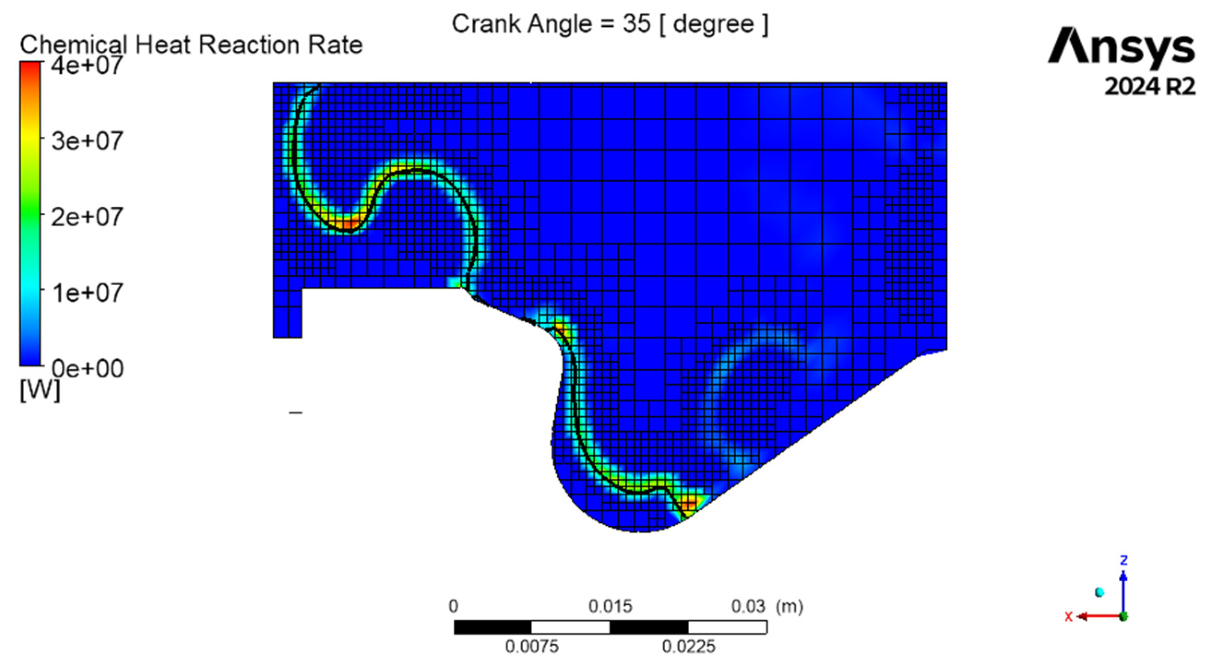
. Figure 1 presents the computational mesh with grid refinement superimposed on the Chemical Heat Release Rate (CHRR) at a crank angle (CA) of 35°ATDC (CA35).

4.5. Converge^®—SAGE Combustion Model

The SAGE model is the implementation of a detailed chemical kinetics solver in Converge^®. This solves detailed chemical kinetics using a set of Chemkin^®-formatted input files. SAGE calculates the reaction rates while the transport equations are handled by the CFD solver [52,53]. This is equivalent to the implementation of detailed chemical kinetics in Forte^®, which uses the ANSYS Chemkin^® chemistry solver ([9], p. 11).

Converge^® offers the implementation of the G-equation model, which can be used independently or in conjunction with SAGE. The G-equation model runs faster than detailed chemistry; however, SAGE allows the user to obtain results for combustion products [52]. In the present work, SAGE was used in Converge^® without the application of the G-equation model.

The attractiveness of the G equation model is that it models and gives information by tracking turbulent flame propagation; therefore, it represents the interaction between the flame boundary and turbulence [14]. Models such as the SAGE model can technically be used when it can be assumed that chemical kinetics dominate and that turbulence plays a lesser role in the combustion process ([14], p. 318). This is because combustion is assumed to occur volumetrically in each computational cell.

SAGE is also similar to the Detailed Chemistry Direct Integration option (DCDI) available in Forte^®, which approach does not involve any flame front surface tracking model. Combustion is simulated by modelling each computational cell as a well-stirred reactor and solving detailed chemical kinetics equations ([54], Section 3.3.4). DCDI is available in the spark ignition model in Forte^®.

5. Simulation Results

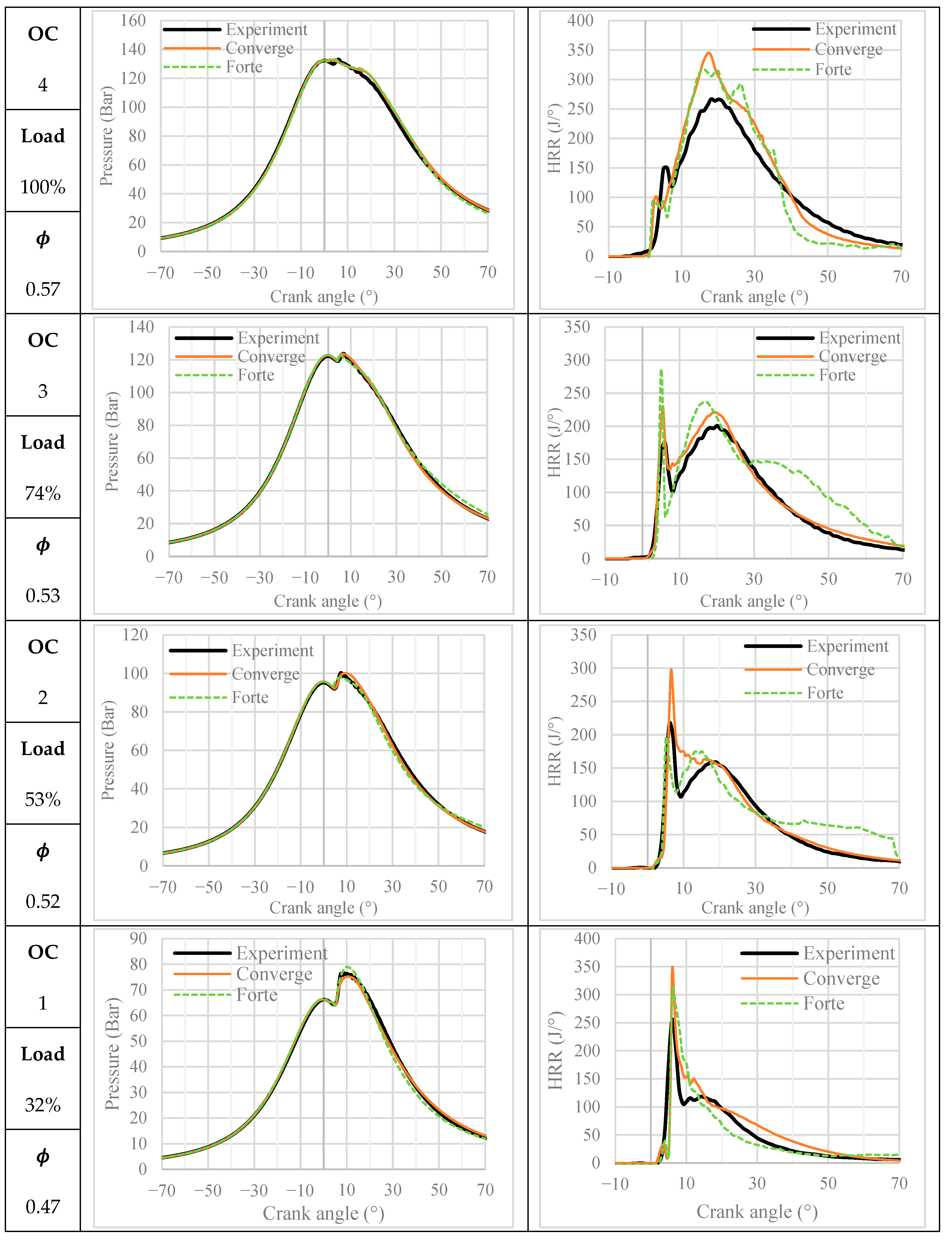
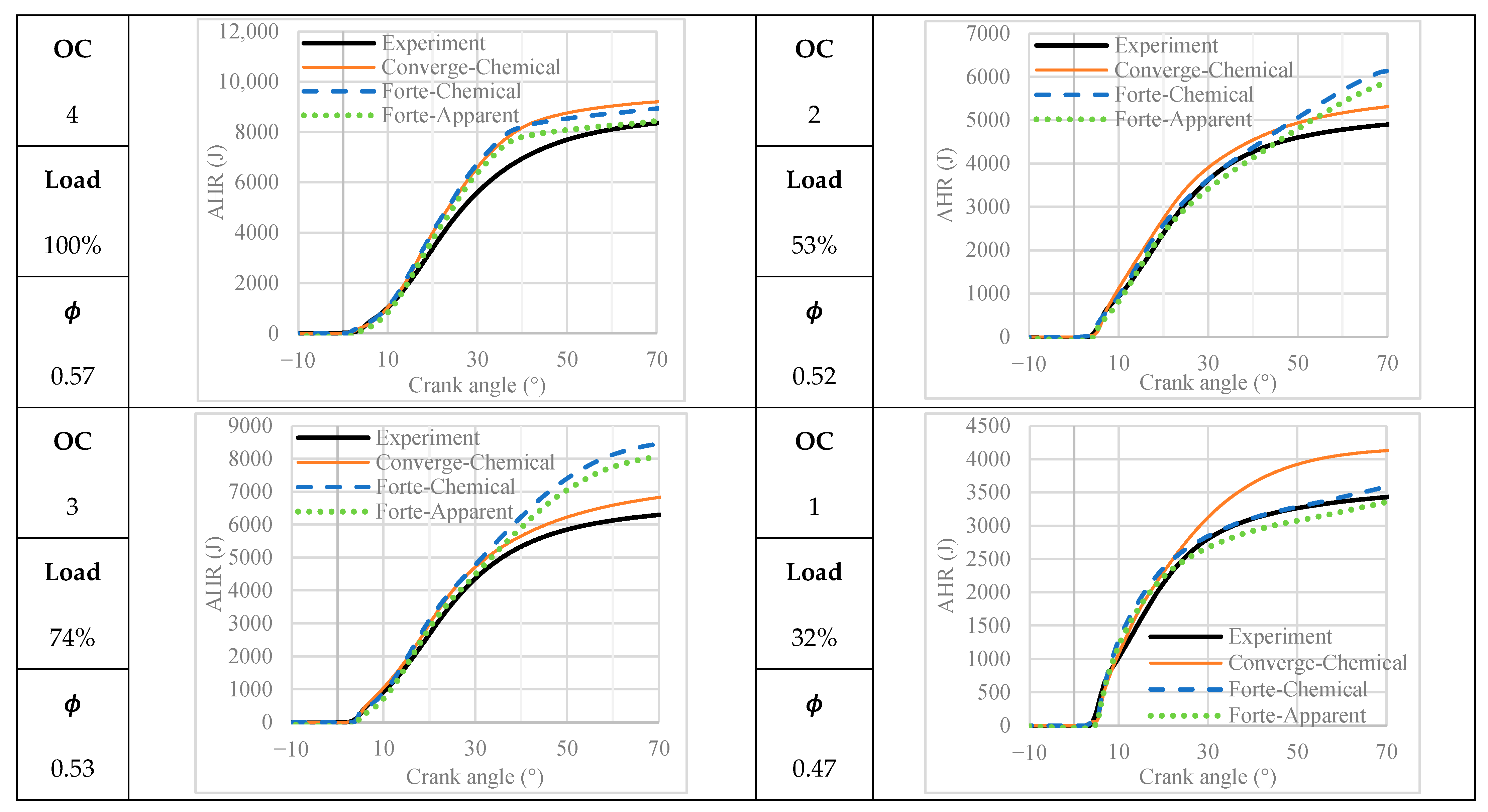
The simulation results from both ANSYS Forte^® and Converge^® are presented in this section. Figure 2 and Figure 3 present in-cylinder pressure, Heat Release Rate (HRR) and Accumulated Heat Release (AHR) superimposed on experimental data for the four operating conditions (OC) described in Table 3. In Figure 3, it is important to distinguish between the heat release definitions. The experimental AHR represents the apparent heat release derived from in-cylinder pressure data. Conversely, the Converge^® AHR represents the chemical heat release, which is the gross heat released by combustion. Hence, to ensure rigorous comparison, Forte^® results include both the chemical AHR and the apparent AHR.

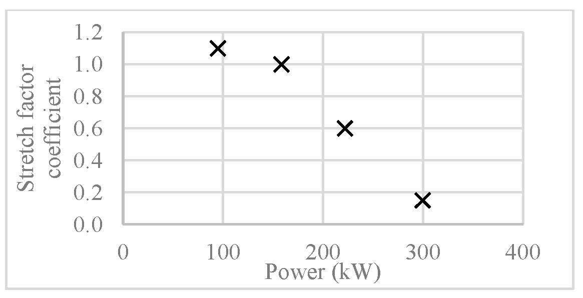
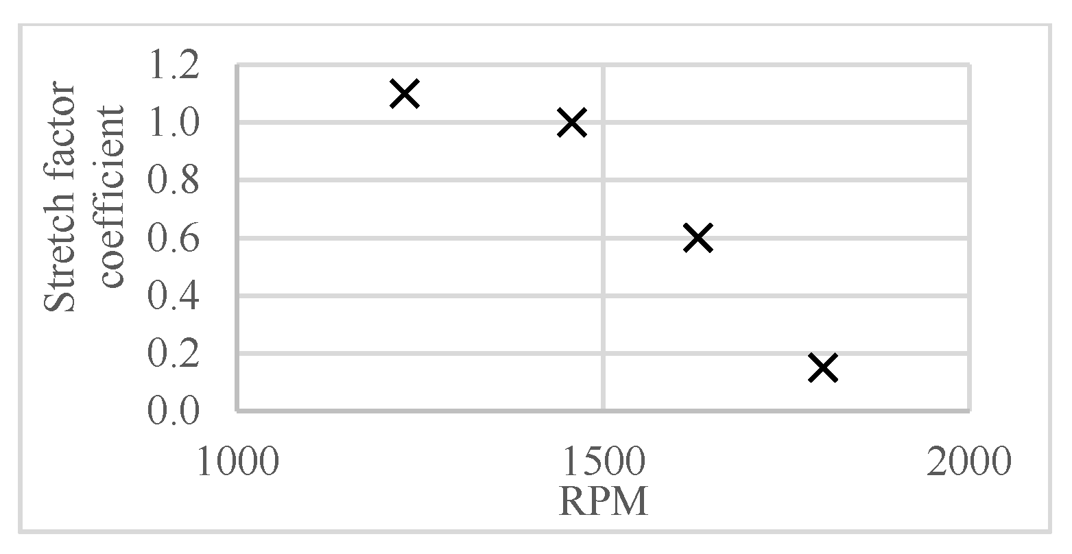
The stretch factor coefficient $C_{ms}$ resulting from the tuning procedure in Forte^®, as described in Section 4, is plotted with engine power and RPM in Figure 4 and Figure 5, respectively. Power and rotational speed are interrelated since the engine was operated under a propulsion characteristics curve in the experiments as described in Section 3.

The ANSYS Forte^® results for 100% and 32% load agreed very well with experimental in-cylinder pressure. Good agreement was also observed for HRR and AHR at 100% load. The Forte^®-apparent AHR matched the experimental (apparent) AHR well. Furthermore, the Forte^®-chemical AHR agreed well with the Converge^® (chemical) AHR. The same can be said for 32% load, although Converge^® predicted slightly higher (chemical) AHR compared to Forte^®-chemical AHR. This was a consequence of the higher HRR predicted in Converge^® between CA20 and CA50. Nonetheless, the pressure predictions show good agreement.

The mid-load simulation results (74% and 53% load) agreed with experimental results up to CA30, but after CA30, the Forte^® HRR was over-predicted compared to both the experimental data and Converge^® results. Consequently, the Forte^® AHR (both chemical and apparent) was higher than experimental and Converge^® values.

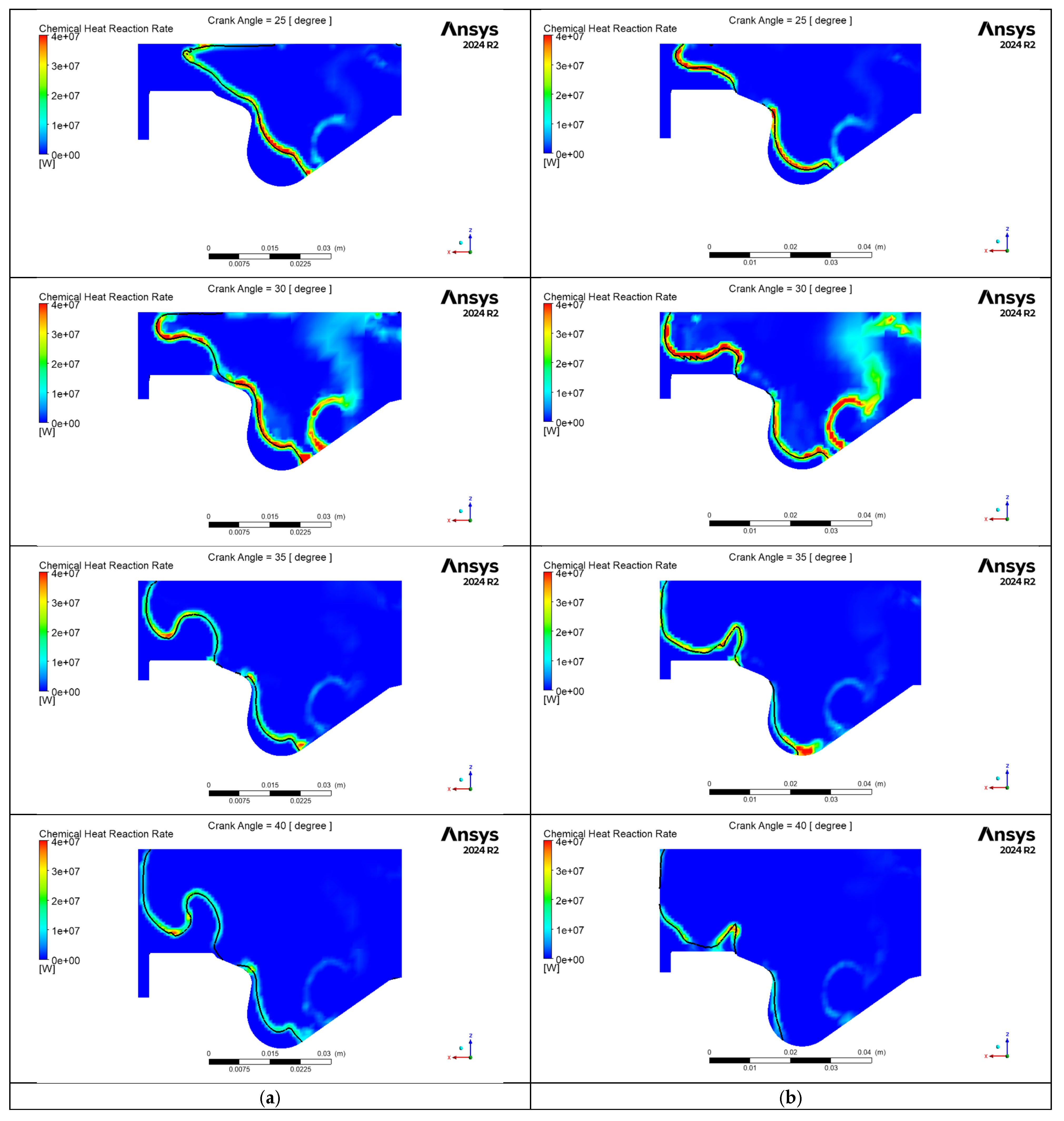
This discrepancy suggests a limitation in the flame quench modelling within this combustion regime. The period between CA30 and CA40 coincides with the flame front reaching the cylinder liner. The persistence of high HRR in the simulation implies that the flame quench model did not sufficiently retard the reaction rate close to the walls. This hypothesis is supported by Figure 6a, which shows the contour plot for Chemical Heat Release Rate (CHRR) at 74% load for a range of CA. The mean flame front is indicated by the black iso-line ($G=0$). The visualisation showed that from CA25 to CA30, the heat release rate increased rather than decreased, contradicting the experimental HRR data shown in Figure 2. This behaviour indicates continued flame propagation towards the wall rather than quenching. Flames may quench due to heat loss to the liner or charge stratification ([9], Section 7.4.5). The latter may not have occurred since the simulation setup assumed a homogeneous mixture of O₂, N₂ and CH₄, neglecting any residual combustion products.

This discrepancy between experimental and Forte^® HRR after CA30 (in mid-load results) may also be an indication that the flame stretch parameter has to vary with combustion in line with what was stated in Section 2.2 (Observations) and in [21]. Simulation trials showed that increasing the flame stretch coefficient in later periods (after CA30) did decrease the HRR, but this could not be concluded since a variable flame stretch coefficient is currently not implemented in Forte^®.

The CHRR depicted in Figure 6 is based on the flame front heat release calculation, which is calculated on sub-grid volume modelling of flame-containing cells as described in Section 4. The result is presented on the larger overall computational mesh, which therefore pixelates the depiction of CHRR. The CHRR computation is valid, and a mesh independence study was conducted.

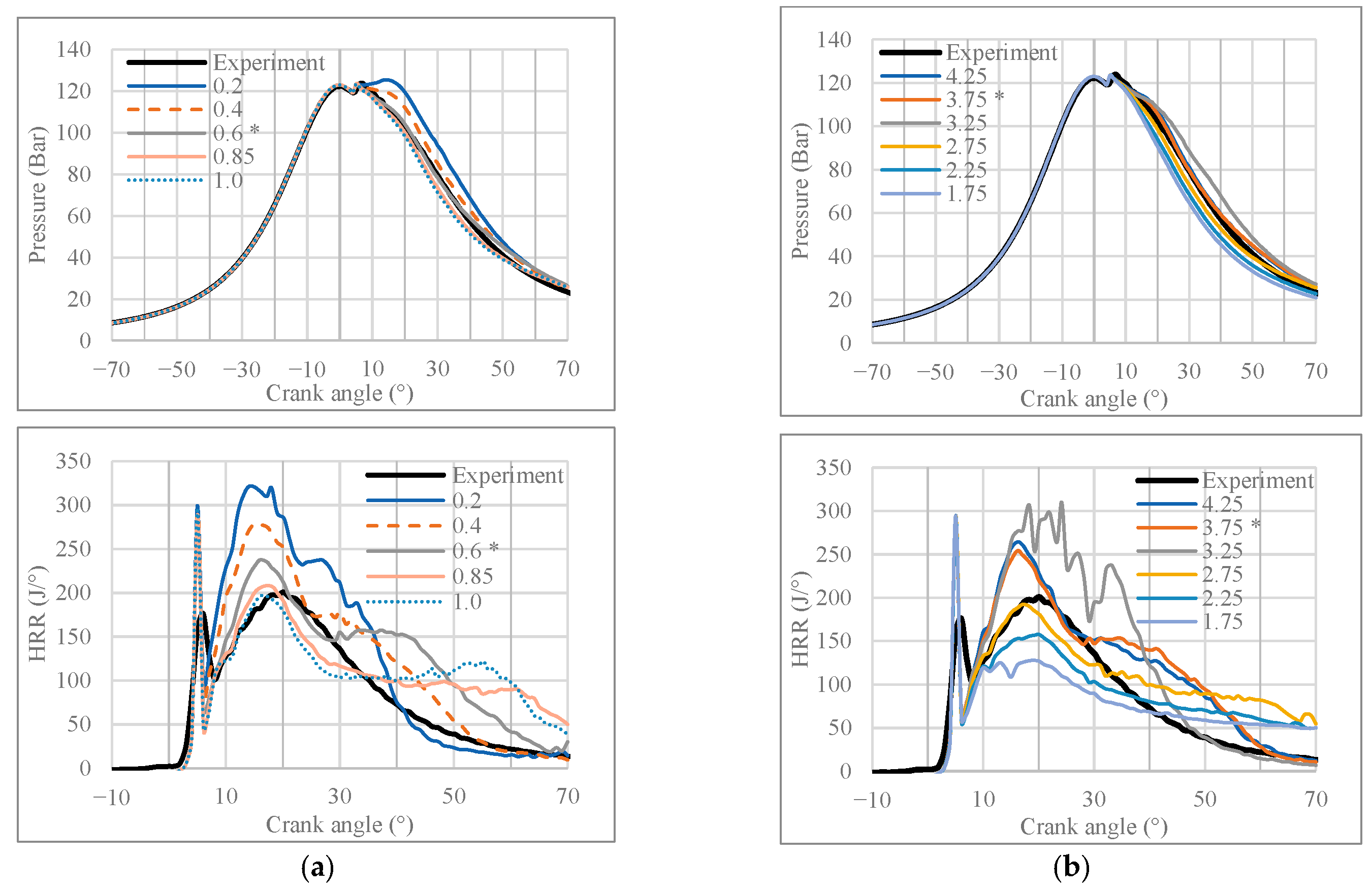
In order to further understand the respective effect of tuning the flame stretch coefficient $C_{ms}$ or the flame speed ratio $b_1$ (in Forte^®), the simulation results for a range of these parameters are now presented for the same engine load condition. Figure 7a shows the effect of varying the flame stretch coefficient $C_{ms}$ on the 74% load simulation. The tuning process yielded an optimal value of $C_{ms}$ = 0.6 to match simulation and experimental HRR. Decreasing $C_{ms}$ results in a faster flame speed (as per Equation (8) for $I_0$) and a respective higher HRR during flame propagation (CA15). Increasing $C_{ms}$ does the opposite. The effects on flame speed are visually confirmed in Figure 6a,b, which show the CHRR and flame front at 74% load with $C_{ms}$ = 0.6 and $C_{ms}$ = 0.2, respectively. The flame front for $C_{ms}$ = 0.2 is more advanced than $C_{ms}$ = 0.6 at any crank angle.

Similarly, Figure 7b presents the effects of changing the flame speed ratio $b_1$ with $C_{ms}$ kept constant at 0.6 (presented for the 74% load). As expected, increasing $b_1$ resulted in a faster flame propagation as shown by the higher HRR at CA20. It is interesting to note that when changing $C_{ms}$ and $b_1$, the elevated HRR after CA30 persisted, indicating that this result from the simulation is not an effect of flame speed parameter tuning. This further supports the conclusion that the late-cycle discrepancy is driven by the wall-interaction and quenching physics rather than the turbulent flame speed calibration.

6. Conclusions

This article presented experimental and simulation results of lean dual-fuel combustion of premixed methane-air mixtures ignited by pilot-injected diesel fuel. The range of methane-air equivalence ratio was 0.47–0.57 across four load conditions (operating conditions).

The simulation In-Cylinder Pressure (ICP) and HRR results of the 100% and 32% load agreed well with experimental results. The AHR for these load conditions presented by the simulations was close to that determined experimentally. Apart from being important for the final heat release, this feature is critical for final combustion product analysis.

The results at 53 and 74% load were also presented, compared and the discrepancy in HRR after CA30 was described and addressed.

The use of the G-equation model presented details of the mean flame front, including the flame propagation, both during computation and post-processing analysis. The drawback of this model was the tuning effort required in the simulation setup.

The variation of the stretch factor coefficient across the range of 4 load conditions was presented. A strong correlation was observed between the methane-air equivalence ratio and the required stretch factor coefficient $C_{ms}$. As the mixture became leaner, the calibrated $C_{ms}$ value increased.

The experimental data involved coupled variation in both load and RPM. Therefore, the variation of the stretch factor coefficient $C_{ms}$ experienced through this simulation campaign cannot be attributed entirely to load or RPM changes. It is known that both load and RPM affect flame propagation and, therefore, flame stretch sensitivity. Following the study presented herein, a continuation of the research is planned, which will collect experimental data from a dual-fuel engine operating with variable-load/fixed-RPM and variable-RPM/fixed-load. This experimental data will be used to perform simulations using the G-equation methodology to further explore the effects of the flame stretch coefficient. That said, load variation is linked to variation in equivalence ratio, and this is thought to be the major contributor to the variation in stretch factor coefficient $C_{ms}.$

It is expected that the variation of flame stretch coefficient came as a result of the significantly lean methane-air equivalence ratios and the use of methane as the premixed gaseous fuel. It is known that methane has a negative Markstein number below an equivalence ratio of 0.9 at atmospheric conditions and a negative Markstein length for $\varphi$ < 1.0 and pressure of 1.0 MPa [27,28,29]. The lean methane-air equivalence ratios are a result of the lean burn combustion concept.

Given methane’s faster diffusivity compared to air, lean equivalence ratios of methane-air mixtures do not have a Lewis number equal to unity and will experience preferential diffusion, leading to changes in the local flame speed.

Due to preferential diffusion, methane is unstable in fuel-lean conditions (due to a negative Markstein number) and stable in fuel-rich conditions (due to a positive Markstein number), ([23], Figure 8). (Methane being the fast-diffusing reactant in methane-air flames). The change in flame stretch factor coefficient $C_{ms}$ in this work was thus large due to the low equivalence ratios.

The change in stretch factor coefficient $C_{ms}$ in the case of propane-air combustion simulation is therefore expected to be reversed since propane has a negative Markstein number at rich equivalence ratios and a positive Markstein number at lean equivalence ratios (Oxygen being the fast-diffusing reactant in propane-air flames), ([23], Figure 7).

Since ethane and ethylene have mass diffusivities intermediate to those of methane and propane, resulting in a reduced response to the effects of stretch [23], combustion simulations with ethane or ethylene-air mixtures are expected to have smaller variation of the flame stretch factor coefficient $C_{ms}$.

The resulting flame stretch factor coefficient used in the present simulations increased with decreasing equivalence ratio. With reference to Equations (7) and (8), an increase in $C_{ms}$ decreases $I_0$ and decreases the modeled turbulent flame speed $S_T$.

The findings on the variation of the flame stretch factor coefficient in this study show the importance of taking into consideration thermo-diffusive effects to account for flame stretch and preferential diffusion during flame propagation in simulation work.

Future work may investigate alternative modelling strategies to better account for such flame instabilities. An improvement could be achieved by integrating a computational routine in the numerical scheme to calculate the near-flame Lewis number and Markstein lengths to directly implement stretch sensitivity effects on flame propagation.

References

- Karim, G.A. Dual-Fuel Diesel Engines; CRC Press: London, UK, 2021. [Google Scholar]
- Weaver, C.S.; Turnier, S.H. Dual Fuel Natural Gas/Diesel Engines: Technology, Performance, and Emissions. In Proceedings of the International Congress and Exposition, Detroit, MI, USA, 28 February–3 March 1994; pp. 77–92, SAE Technical Paper 940548. [Google Scholar] [CrossRef] [Scilit]
- Heywood, J. Internal Combustion Engine Fundamentals, 2nd ed.; McGraw Hill Professional: New York, NY, USA, 2018. [Google Scholar]
- De Robbio, R.; Cameretti, M.C.; Mancaruso, E.; Tuccillo, R.; Vaglieco, B.M. Combined CFD—Experimental Analysis of the In-Cylinder Combustion Phenomena in a Dual Fuel Optical Compression Ignition Engine; SAE Technical Paper Series; SAE International: Warrendale, PA, USA, 2021; SAE Technical Paper 2021-24-0012. [Google Scholar] [CrossRef] [Scilit]
- De Robbio, R.; Mancaruso, E. Hydrogen combustion analysis via infrared and visible optical diagnostics combined with CFD in a dual fuel engine at low load. Int. J. Hydrogen Energy 2024, 81, 418–435. [Google Scholar] [CrossRef] [Scilit]
- de Oliveira, A.; Yang, J.; Sodré, J.R. Numerical and experimental study on the impact of mild cold exhaust gas recirculation on exhaust emissions in a biodiesel-fueled diesel engine. J. Eng. Gas Turbines Power 2021, 143, 111014. [Google Scholar] [CrossRef] [Scilit]
- Cameretti, M.C.; De Robbio, R.; Mancaruso, E.; Palomba, M. CFD study of dual fuel combustion in a research diesel engine fueled by hydrogen. Energies 2022, 15, 5521. [Google Scholar] [CrossRef] [Scilit]
- Puduppakkam, K.V.; Liang, L.; Naik, C.V.; Meeks, E.; Kokjohn, S.L.; Reitz, R.D. Use of detailed kinetics and advanced chemistry-solution techniques in CFD to investigate dual-fuel engine concepts. SAE Int. J. Engines 2011, 4, 1127–1149. [Google Scholar] [CrossRef] [Scilit]
- Ansys. Forte Theory Manual—2023 R2; Ansys: Canonsburg, PA, USA, 2023. [Google Scholar]
- Verma, I.; Bish, E.; Kuntz, M.; Meeks, E.; Puduppakkam, K.; Naik, C.; Liang, L. CFD Modeling of Spark Ignited Gasoline Engines—Part 1: Modeling the Engine Under Motored and Premixed-Charge Combustion Mode; SAE Technical Paper Series; SAE International: Warrendale, PA, USA, 2016; SAE Technical Paper 2016-01-0591. [Google Scholar] [CrossRef] [Scilit]
- Heywood, J.B. Internal Combustion Engine Fundamentals; McGraw-Hill Education: New York, NY, USA, 1989. [Google Scholar]
- Poinsot, T.; Veynante, D. Theoretical and Numerical Combustion; Éditions du Becquart: Albi, France, 2022; ISBN 9782746639904. [Google Scholar]
- Abraham, J.; Williams, F.A.; Bracco, F.V. A Discussion of Turbulent Flame Structure in Premixed Charges; SAE Technical Paper Series; SAE International: Warrendale, PA, USA, 1985; SAE Technical Paper 850345. [Google Scholar] [CrossRef] [Scilit]
- Han, Z. Simulation and Optimization of Internal Combustion Engines; SAE International: Warrendale, PA, USA, 2021. [Google Scholar]
- Karlovitz, B.; Denniston, D.W., Jr.; Knapschaefer, D.H.; Wells, F.E. Studies on turbulent flames. Symp. Int. Combust. 1953, 4, 613–620. [Google Scholar] [CrossRef] [Scilit]
- Bray, K.N.C. Turbulent flows with premixed reactants. In Topics in Applied Physics; Springer: Berlin/Heidelberg, Germany, 1980; pp. 115–183. [Google Scholar]
- Williams, F.A. A review of some theoretical considerations of turbulent flame structure. In AGARD Conference Proceedings No. 164 on Analytical and Numerical Methods for Investigation of Flow Fields with Chemical Reactions, Especially Related to Combustion; AGARD: Neuilly-sur-Seine, France, 1975. [Google Scholar]
- Markstein, G.H. Nonsteady Flame Propagation; Pergamon Press: Oxford, UK, 1964. [Google Scholar]
- Williams, F.A. Combustion Theory, 2nd ed.; Benjamin-Cummings Publishing Company: San Francisco, CA, USA, 1985. [Google Scholar]
- Oppong, F.; Luo, Z.; Li, X.; Song, Y.; Xu, C. Intrinsic instability of different fuels spherically expanding flames: A review. Fuel Process. Technol. 2022, 234, 107325. [Google Scholar] [CrossRef] [Scilit]
- Brequigny, P.; Halter, F.; Mounaïm-Rousselle, C.; Dubois, T. Fuel performances in Spark-Ignition (SI) engines: Impact of flame stretch. Combust. Flame 2016, 166, 98–112. [Google Scholar] [CrossRef] [Scilit]
- Brequigny, P.; Halter, F.; Mounaïm-Rousselle, C.; Moreau, B.; Dubois, T. Thermodiffusive Effect on the Flame Development in Lean Burn Spark Ignition Engine; SAE Technical Paper Series; SAE International: Warrendale, PA, USA, 2014; SAE Technical Paper 2014-01-2630. [Google Scholar] [CrossRef] [Scilit]
- Tseng, L.-K.; Ismail, M.A.; Faeth, G.M. Laminar burning velocities and Markstein numbers of hydrocarbonair flames. Combust. Flame 1993, 95, 410–426. [Google Scholar] [CrossRef] [Scilit]
- Brequigny, P.; Mounaïm-Rousselle, C.; Halter, F.; Moreau, B.; Dubois, T. Impact of Fuel Properties and Flame Stretch on the Turbulent Flame Speed in Spark-Ignition Engines; SAE Technical Paper Series; SAE International: Warrendale, PA, USA, 2013; SAE Technical Paper 2013-24-0054. [Google Scholar] [CrossRef] [Scilit]
- Egolfopoulos, F.N.; Law, C.K. An experimental and computational study of the burning rates of ultra-lean to moderately-rich H2/O2/N2 laminar flames with pressure variations. Symp. Int. Combust. 1991, 23, 333–340. [Google Scholar] [CrossRef] [Scilit]
- Egolfopoulos, F.N.; Law, C.K. Chain mechanisms in the overall reaction orders in laminar flame propagation. Combust. Flame 1990, 80, 7–16. [Google Scholar] [CrossRef] [Scilit]
- Matalon, M. Flame dynamics. Proc. Combust. Inst. 2009, 32, 57–82. [Google Scholar] [CrossRef] [Scilit]
- Gu, X.J.; Haq, M.Z.; Lawes, M.; Woolley, R. Laminar burning velocity and Markstein lengths of methane–air mixtures. Combust. Flame 2000, 121, 41–58. [Google Scholar] [CrossRef] [Scilit]
- Li, H.; Xiao, H.; Sun, J. Laminar burning velocity, Markstein length, and cellular instability of spherically propagating NH3/H2/Air premixed flames at moderate pressures. Combust. Flame 2022, 241, 112079. [Google Scholar] [CrossRef] [Scilit]
- Manton, J.; von Elbe, G.; Lewis, B. Nonisotropic propagation of combustion waves in explosive gas mixtures and the development of cellular flames. J. Chem. Phys. 1952, 20, 153–157. [Google Scholar] [CrossRef] [Scilit]
- Aleiferis, P.G.; Serras-Pereira, J.; Richardson, D. Characterisation of flame development with ethanol, butanol, iso-octane, gasoline and methane in a direct-injection spark-ignition engine. Fuel 2013, 109, 256–278. [Google Scholar] [CrossRef] [Scilit]
- Xiang, L. Marine Dual Fuel Engines Modelling and Optimisation Employing a Novel Combustion Characterisation Method. Ph.D. Thesis, University of Strathclyde, Glasgow, UK, 2021. [Google Scholar]
- Han, Z.; Reitz, R.D. Turbulence modeling of internal combustion engines using RNG κ-ε models. Combust. Sci. Technol. 1995, 106, 267–295. [Google Scholar] [CrossRef] [Scilit]
- Ansys. Forte Best Practices—2023 R2; Ansys: Canonsburg, PA, USA, 2023. [Google Scholar]
- Saliba, A.T.; Mollicone, J.P.; Scerri, K.; Farrugia, M. Characterisation of Diesel Fuel Injection Rate Profile by Means of a Metaheuristic Approach. In 2024 Industrial Simulation Conference; Universitat Politecnica de Valencia: Valencia, Spain, 2024. [Google Scholar]
- Williams, F.A. Turbulent combustion. In The Mathematics of Combustion; Buckmaster, J.D., Ed.; Society for Industrial and Applied Mathematics: Philadelphia, PA, USA, 1985. [Google Scholar]
- Peters, N. Turbulent Combustion; Cambridge University Press: Cambridge, UK, 2000. [Google Scholar]
- Tan, Z.; Reitz, R.D. An ignition and combustion model based on the level-set method for spark ignition engine multidimensional modeling. Combust. Flame 2006, 145, 1–15. [Google Scholar] [CrossRef] [Scilit]
- Liang, L.; Reitz, R.D. Spark Ignition Engine Combustion Modeling Using a Level Set Method with Detailed Chemistry; SAE Technical Paper Series; SAE International: Warrendale, PA, USA, 2006; SAE Technical Paper 2006-01-0243. [Google Scholar] [CrossRef] [Scilit]
- Liang, L.; Reitz, R.D.; Iyer, C.O.; Yi, J. Modeling Knock in Spark-Ignition Engines Using a G-Equation Combustion Model Incorporating Detailed Chemical Kinetics; SAE Technical Paper Series; SAE International: Warrendale, PA, USA, 2007; SAE Technical Paper 2007-01-0165. [Google Scholar] [CrossRef] [Scilit]
- Herweg, R.; Maly, R.R. A Fundamental Model for Flame Kernel Formation in SI Engines; SAE Technical Paper Series; SAE International: Warrendale, PA, USA, 1992; SAE Technical Paper 922243. [Google Scholar] [CrossRef] [Scilit]
- Liu, J.; Szybist, J.; Dumitrescu, C. Choice of Tuning Parameters on 3D IC Engine Simulations Using G-Equation; SAE Technical Paper Series; SAE International: Warrendale, PA, USA, 2018; SAE Technical Paper 2018-01-0183. [Google Scholar] [CrossRef] [Scilit]
- Singh, S.; Liang, L.; Kong, S.-C.; Reitz, R.D. Development of a flame propagation model for dual-fuel partially premixed compression ignition engines. Int. J. Engine Res. 2006, 7, 65–75. [Google Scholar] [CrossRef] [Scilit]
- Liang, L. Multidimensional Modeling of Combustion and Knock in Spark-Ignition Engines with Detailed Chemical Kinetics. Ph.D. Thesis, University of Wisconsin-Madison, Madison, WI, USA, 2006. [Google Scholar]
- ANSYS. ANSYS Chemkin-Pro Theory Manual—2023 R1; ANSYS: Canonsburg, PA, USA, 2023. [Google Scholar]
- Rahimi, A.; Fatehifar, E.; Saray, R.K. Development of an optimized chemical kinetic mechanism for homogeneous charge compression ignition combustion of a fuel blend of n-heptane and natural gas using a genetic algorithm. Proc. Inst. Mech. Eng. Pt. D J. Automob. Eng. 2010, 224, 1141–1159. [Google Scholar] [CrossRef] [Scilit]
- Liu, L.; Liu, S.; Xia, Q.; Liu, B.; Ma, X. Numerical investigation on mixing characteristics and mechanism of natural gas/air in a super-large-bore dual-fuel marine engine. Atmosphere 2022, 13, 1528. [Google Scholar] [CrossRef] [Scilit]
- Nazemian, M.; Nazemian, M. A Holistic Approach to Reactivity-Controlled Compression Ignition Engine Performance: 4E Analysis (Evaporation, Energy, Emissions, Exergy) and Multidimensional Efficiency Metrics under Varying Engine Speed. Automot. Sci. Eng. 2025, 15, 4704–4738. [Google Scholar] [CrossRef]
- Altinkurt, M.D.; Coskun, G.; Tunér, M.; Turkcan, A. A comprehensive investigation of early pilot (e-pilot) mode split injection variations for improving NG-diesel dual-fuel combustion in a medium-speed marine engine: Experiments and CFD study. Case Stud. Therm. Eng. 2025, 68, 105881. [Google Scholar] [CrossRef] [Scilit]
- Wijeyakulasuriya, S.; Jupudi, R.S.; Givler, S.; Primus, R.J.; Klingbeil, A.E.; Raju, M.; Raman, A. Multidimensional modeling and validation of dual-fuel combustion in a large bore medium speed diesel engine. In Proceedings of the ASME 2015 Internal Combustion Engine Division Fall Technical Conference, Houston, TX, USA, 8–11 November 2015; Volume 1: Large Bore Engines; Fuels; Advanced Combustion. Paper No: ICEF2015-1077, V001T01A006. 14p. [Google Scholar] [CrossRef] [Scilit]
- Pomraning, E.; Richards, K.; Senecal, P.K. Modeling Turbulent Combustion Using a RANS Model, Detailed Chemistry, and Adaptive Mesh Refinement; SAE Technical Paper Series; SAE International: Warrendale, PA, USA, 2014; SAE Technical Paper 2014-01-1116. [Google Scholar] [CrossRef] [Scilit]
- Converge CFD Software. Converge 3.1 Manual; Converge CFD: Madison, WI, USA, 2023. [Google Scholar]
- Senecal, P.K.; Pomraning, E.; Richards, K.J.; Briggs, T.E.; Choi, C.Y.; McDavid, R.M.; Patterson, M.A. Multi-Dimensional Modeling of Direct-Injection Diesel Spray Liquid Length and Flame Lift-Off Length Using CFD and Parallel Detailed Chemistry; SAE Technical Paper Series; SAE International: Warrendale, PA, USA, 2003; SAE Technical Paper 2003-01-1043. [Google Scholar] [CrossRef] [Scilit]
- Ansys. Forte User’s Guide—2023 R2; Ansys: Canonsburg, PA, USA, 2023. [Google Scholar]
Figure 1.
Computational mesh superimposed on CHRR (Forte®).
Figure 2.
Simulation and experimental results—Converge® (SAGE), Forte® (G-equation).
Figure 3.
Accumulated Heat Release (AHR), simulation and experimental results—Converge® (SAGE), Forte® (G-equation).
Figure 4.
Stretch factor coefficient with engine power.
Figure 5.
Stretch factor coefficient with engine RPM.
Figure 6.
Simulation contour plot of CHRR (Forte®) at 74% power at different crank angle intervals. (a) [ = 0.6, = 3.75]. (b) [ = 0.2, = 3.75].
Figure 7.
Simulation results (Forte®). (a) with different stretch factor coefficient [With = 3.75]; (b) with different turbulent flame speed ratio [With = 0.6]. (*) indicates the optimal value determined through the tuning procedure.