Carbon Trading-Driven Optimal Collaborative Scheduling of Integrated Energy Systems with Multiple Flexible Loads

Abstract

To address the challenges associated with energy decarbonization and economic operation in integrated energy systems (IESs), this paper proposes a collaborative optimal dispatch strategy for IES that considers multiple flexible loads under a carbon trading mechanism. First, a mathematical model of user-side loads is constructed according to the characteristics of flexible loads. Second, a comprehensive optimization framework is constructed by embedding the carbon trading mechanism into the IES operational model. The objective function minimizes the total operating costs, including energy purchase costs, fuel costs, carbon trading costs, operation and maintenance costs, compensation costs, and green certificate revenues. The CPLEX solver is then employed to solve the model. Finally, a case study is conducted to validate the proposed method. Simulation results demonstrate that the carbon trading mechanism effectively leverages the demand response capabilities and coordinates multiple resources, including electricity, heat, and storage, thereby achieving low-carbon economic operation of the system.

1. Introduction

The development and efficient utilization of integrated energy, along with multi-energy complementarity, are pivotal for improving energy efficiency and protecting the environment [1]. The integrated energy system (IES), characterized by multi-energy complementarity, intelligent configuration, and optimized dispatching, has become a key technology for driving the energy structure transformation and achieving low-carbon emission strategic goals. By leveraging various energy carriers, such as electricity, heat, gas, and transmission networks, the IES provides critical support for the high-efficiency use of distributed energy, as well as for reducing energy costs and carbon emissions [2,3,4].

In the context of the low-carbon policies, it is of great significance to study the impact of carbon emission trading on IES [5,6,7]. For years, there have been extensive explorations conducted by both academia and industry from the supply and demand sides [8,9,10]. On the supply side, the carbon trading mechanism, as an effective policy tool, guides power generation entities to optimize their output and promotes the accommodation of renewable energy by imposing an economic cost on carbon emissions. Reference [11] successfully balanced the system’s economic and low-carbon benefits by freely allocating initial carbon emission permits and calculating the actual carbon emission costs. Reference [12] incorporated the carbon trading mechanism into a virtual power plant and utilized the baseline method to allocate carbon quotas, significantly improving the level of renewable energy accommodation. On the demand side, demand response (DR), as a key technology for enhancing supply-demand interaction and tapping the potential of the demand side, has also garnered significant attention. Researchers have verified the immense potential of DR in alleviating peak shaving pressure and improving energy utilization efficiency by introducing a price elasticity matrix [13], establishing coupled electricity-gas-heat DR models [14], and refining load types (e.g., curtailable, shiftable, substitutable) while considering user satisfaction [15]. Reference [16] introduced multi-energy devices, such as combined heat and power (CHP) units, to facilitate electric-heat demand response. This study achieved economic dispatch of multi-energy parks, improved renewable energy accommodation, and reduced system losses. Reference [17] developed an integrated demand response model covering electricity, heat, and cooling loads, achieving optimal operational scheduling via a Stackelberg game framework. Focusing on building integrated energy systems, Reference [18] proposed an energy management optimization model wherein cooling and heating loads are subject to tiered subsidies, and electric loads participate in price-based integrated demand response. By incorporating demand response subsidies in the objective function, this approach comprehensively accounts for user comfort and energy expenditure, ultimately improving the economic benefits for both the system and its users.

However, there are several limitations among the existing research. Most studies either focus solely on the impact of the carbon trading mechanism on the supply side or independently analyze the application of demand response, failing to organically integrate them together to synergistically optimize the system’s low-carbon and economic performance. Reference [19] proposed a low-carbon economic operation optimization scheduling model for integrated energy systems that considers a tiered carbon trading mechanism and demand-side response. Reference [20] investigated the coordinated optimal scheduling of multiple integrated energy systems under a dynamic carbon-green certificate trading mechanism, aiming to improve the low-carbon economic efficiency and resource supply-demand flexibility of integrated energy systems incorporating electricity, heat, and gas. Although some studies have focused on integrated electricity and heat energy systems (IEHS) [21,22], they often suffered from insufficient refinement of the demand-side models. For instance, Reference [22] proposed an integrated demand-side response scheme but failed to construct a refined load model that could fully reflect the diversity of user energy consumption behavior. In recent years, research on community-level IES based on the Energy Hub (EH) model [23,24], despite having recognized the scheduling value of flexible loads [25], still lacks a unified dynamic response framework that encompasses multiple load characteristics, such as shiftable, transferable, and curtailable loads, under the carbon trading mechanism. Consequently, there is a need to achieve optimal scheduling of integrated energy systems that integrate user-side flexible load demand response within the context of carbon trading.

To address the limitations associated with low-carbon and economic performance, this paper proposes a coordinated optimal dispatch strategy for integrated energy systems with diverse flexible loads under a carbon trading mechanism, achieved by synergistically fusing carbon trading and user-side demand responses. The main contributions are as follows:

(1)

Comprehensive modeling of multi-type flexible loads. Mathematical models for shiftable, transferable, and curtailable loads are formulated, providing a comprehensive and practical framework for characterizing user-side flexible resources in the IES.

(2)

Multi-objective economic framework integrating carbon trading and green certificates. This work constructs a comprehensive cost model that combines energy purchase, fuel, carbon trading, operation and maintenance, and compensation costs. Distinct from existing literature, this model explicitly incorporates green certificate revenue (with a specific sign definition) into the objective function, thereby establishing a synergistic mechanism to enhance both economic and low-carbon performance.

(3)

A coordinated optimal dispatch strategy under tiered carbon pricing. This work employs a strict tiered carbon trading mechanism where pricing rules are consistently applied regardless of interval length. By embedding this mechanism with flexible load constraints into a coordinated dispatch model, the proposed strategy effectively minimizes total operating costs while maximizing system flexibility.

The remainder of this paper is organized as follows: Section 2 presents the integrated energy system and flexible load models. The carbon trading mechanism is presented in Section 3. A collaborative optimization model of IES under a carbon trading mechanism is described in Section 4. In Section 5, a case study is conducted, and the results are discussed. Finally, the conclusion is drawn in Section 6.

2. Integrated Energy System and Flexible Load Models

2.1. Integrated Energy System

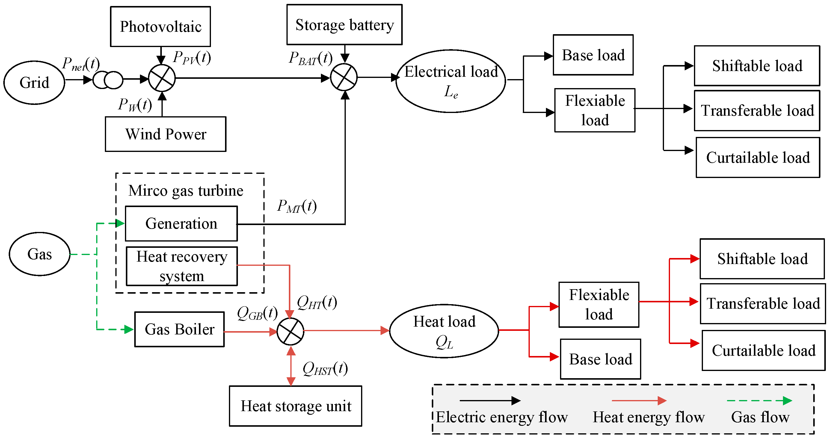
To accurately characterize the coupling relationships of multi-energy flows within the community integrated energy system, this work introduces a mathematical model based on the Energy Hub (EH) theory [23,24]. This model treats the entire system as a multi-input, multi-output energy conversion and distribution unit, as illustrated in Figure 1. It comprehensively encompasses the four core links of the system: energy input, conversion, storage, and output, thereby laying the foundation for subsequent optimal scheduling analysis.

In this EH model, energy inputs are primarily derived from the upper-level grid, local distributed energy resources (such as photovoltaic and wind power), and natural gas. The energy conversion link consists of transformers and micro gas turbines (MT). The transformer converts high-voltage electricity into low-voltage electricity suitable for end-users, while the MT facilitates combined heat and power (CHP) generation by combusting natural gas. Its output electricity supplies the electrical load, while its recovered heat supplies the heat load.

Energy output in the IES is achieved through the coordination of multiple devices. Electricity is jointly supplied by the transformer and the MT generation system, whereas heat output is provided by the waste heat recovery system of the MT and the gas boiler (GB). To smooth energy fluctuations and enhance operational flexibility, the model also incorporates an energy storage link, including batteries for electrical energy storage and heat storage tanks for heat energy.

2.2. Flexible Load Characteristic Analysis

In integrated energy systems, system output is primarily utilized to meet the diversified load demands of users. To accurately quantify the potential of user-side demand response, this work categorizes user-side loads into four fundamental types based on their adjustment modes and physical characteristics: base loads, shiftable loads, curtailable loads, and transferable loads. Among these, base loads, also referred to as rigid loads, are not subject to any form of scheduling intervention by the system; the others are classified as flexible loads, and the models of which are described as follows.

2.2.1. Shiftable Load Model

Shiftable loads refer to loads for which the execution time of tasks can be shifted backward or forward as a whole. Their core characteristics are that during the shifting process, both the power profile and the duration of the load remain unchanged, and task execution is non-interruptible. Typical applications include periodic appliances such as washing machines and dishwashers.

Let the unit scheduling period be 1 h. For a specific shiftable load $L_{shift}^{t,x}$, its power distribution vector before participating in scheduling can be expressed as follows:

$$L_{shift}^{t,x}=\left(0,\dots ,P_t^{shift,x},P_{t+1}^{shift,x},P_{t+t_D}^{shift,x},\dots ,0\right)$$

(1)

where the superscript x denotes the load type (i.e., x ∈ {e: electric load, h: heat load}), and t represents the starting time; $P_t^{shift,x}$ represents the power of the load at time t; and t_D is the execution duration.

To accurately describe the scheduling behavior of shiftable loads, this work introduces a binary decision variable to characterize their start times. Assume that the allowable shifting time window for a shiftable load $L_{shift}^{\tau ,x}$ is $\left[t_{sh}^{-}, t_{sh}^{+}\right]$. To indicate whether the load starts at a specific moment, a binary decision variable ${\alpha }_t^x$ is defined, where ${\alpha }_t^x$ = 1 indicates that $L_{shift}^{\tau ,x}$ starts at time τ; ${\alpha }_t^x$ = 0 indicates that $L_{shift}^{\tau ,x}$ is not shifted. Thus, the set of possible start periods $S_{shift}^x$ is expressed as follows:

$$S_{shift}^x=\left[t_{sh}^{-},t_{sh}^{+}-t_D+1\right], t_{sh}^{+}-t_{sh}^{-}>t_D$$

(2)

If τ = t, the load remains unchanged; if τ ∈ $\left[t_{sh}^{-},t_{sh}^{+}-t_D+1\right]$ and τ ≠ t, the power distribution vector shifted from the original start period t to the new start period τ is as follows:

$$L_{shift}^{\tau ,x}=\left(0,\dots ,P_{\tau }^{shift,x},P_{\tau +1}^{shift,x},P_{\tau +t_D}^{shift,x},\dots ,0\right)$$

(3)

Therefore, during the shifting process, the shiftable load does not alter the power magnitude, but only the timing; this can be described as follows:

$${\displaystyle \sum _{t=\tau }^{\tau +t_D-1}\left(L_{shift}^{\tau ,x}-L_{shift}^{t,x}\right)}=0$$

(4)

To incentivize users actively participate in balancing supply and demand, and to remunerate them for any financial losses or additional costs caused by modifying their electricity usage or production plans, the compensation cost $f_{shift}^x$ paid to the user after load shifting is as follows:

$$f_{shift}^x={\lambda }_{cost}^{shift,x}{\displaystyle \sum _{t=1}^T{\alpha }_t^x{P}_t^{shift,x}}$$

(5)

where ${\lambda }_{cost}^{shift,x}$ represents the compensation coefficient per unit power for a shiftable load of type x; T is the number of time intervals in a day, with T = 24.

2.2.2. Transferable Load Model

Transferable loads are the most flexible type of loads. Their core characteristic is that the power consumption within each scheduling period can be adjusted, and task execution is allowed to be interrupted. The primary constraint is that the total energy demand remains constant throughout the entire scheduling cycle. For instance, the charging behavior of Electric Vehicles (EVs) under orderly charging mode is a typical representative of this category.

Assume the transfer time interval for a transferable load $L_{tran}^x$ is $\left[t_{tr}^{-}, t_{tr}^{+}\right]$. A binary variable ${\beta }_t^x$ is used to indicate the transfer state of $L_{tran}^x$ at a specific time t, where ${\beta }_t^x$ = 1 indicates that the power $P_t^{tran}$ in $L_{tran}^x$ is transferred at time t. The constraint on the transferred power is defined as follows:

$${\beta }_t^x{P}_{\min }^{tran,x}\le P_t^{tran,x}\le {\beta }_t^x{P}_{\max }^{tran,x}$$

(6)

where $P_{\min }^{tran,x}$ and $P_{\max }^{tran,x}$ represent the minimum and maximum power limits of the transferable load with type x, respectively.

For transferable loads, relying solely on the total energy conservation without additional constraints may logically result in frequent start-stop operations across multiple discontinuous periods, thereby affecting the lifespan of equipment. Therefore, to ensure the engineering feasibility of the scheduling scheme, it is necessary to impose a minimum continuous operation time constraint:

$${\displaystyle \sum _{\tau =t}^{t+T_{\min }^{tran,x}-1}{\beta }_{\tau }^x}\ge T_{\min }^{tran,x}$$

(7)

where $T_{\min }^{tran,x}$ represents the minimum continuous operation time.

Similarly, the compensation cost $f_{tran}^x$ paid to the user for transferable loads is calculated as follows:

$$f_{tran}^x={\lambda }_{cost}^{tran,x}{\displaystyle \sum _{t=1}^T\left({\beta }_t^x{P}_t^{tran,x}\right)}$$

(8)

where ${\lambda }_{cost}^{tran,x}$ represents the compensation coefficient per unit power for transferable load of type x.

2.2.3. Curtailable Load Model

Curtailable loads refer to loads that users are willing to accept a power interruption or a reduction in power levels during specific periods in response to scheduling commands. Regulating these loads typically involves a trade-off with partial user comfort. Typical examples include air conditioners, lighting systems, and certain industrial production equipment.

Unlike shiftable or transferable loads, the defining characteristic of curtailable loads is the modification of the user’s total electricity consumption, rather than merely shifting the time of use. To characterize this behavior in an optimization model, a binary decision variable ${\gamma }_t^x$ is introduced to indicate the curtailing state of the load $L_{cut}^x$ at time t.

Let $P_t^{cut,x}$ represent the power of the load at time t participating in scheduling. Load curtailment will incur economic losses and comfort degradation for users, with the magnitude of such losses increasing in proportion to the curtailment level. Therefore, it is necessary to impose power constraints on the curtailable loads, expressed as follows:

$$0\le P_t^{cut,x}\le P_{t,\max }^{cut,x}={\alpha }_{cut}^x{P}_{t,total}^x$$

(9)

where $P_{t,\max }^{cut,x}$ is the maximum power of the curtailable load; ${\alpha }_{cut}^x$ is a proportionality coefficient; $P_{t,total}^x$ denotes the total load at time t.

Similarly, the compensation cost $f_{cut}^x$ paid to the user for load curtailment is calculated as follows:

$$f_{cut}^x={\lambda }_{cost}^{cut,x}{\displaystyle \sum _{t=1}^T{P}_t^{cut,x}}$$

(10)

where ${\lambda }_{cost}^{cut.x}$ denotes the compensation coefficient per unit power for the curtailable load of type x.

3. Carbon Trading Mechanism

The carbon trading mechanism takes the carbon emission allowances as tradable commodities in the carbon market [19,26]. Its implementation effectively promotes carbon emission reduction and improves energy efficiency, thereby mitigating greenhouse gas emissions. In general, government authorities allocate carbon emission quotas to various emission sources. If an entity’s actual carbon emissions are within its allocated quota, the surplus quota can be sold in the market for profits; conversely, if emissions exceed the quota, the deficit carbon allowances have to be purchased from the market. Driven by the objective of maximizing economic benefits, carbon-emitting enterprises are incentivized to adopt effective energy conservation and emission reduction measures.

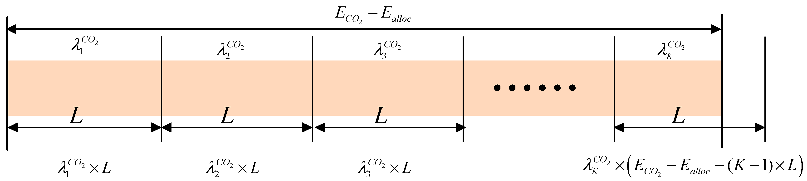
To encourage IES participation in the carbon market, this work introduces a strategy allowing for the independent trading of carbon emission quotas. Specifically, if actual carbon emissions are lower than the allocated quota, the surplus quotas can be sold at market prices to obtain economic returns; conversely, any deficit must be offset by purchasing carbon allowances from the market. Therefore, the carbon trading cost can be expressed:

$$f_{C{O}_2}={\lambda }_{base}^{C{O}_2}\left(E_{C{O}_2}-E_{alloc}\right)$$

(11)

where $f_{C{O}_2}$ denotes the carbon trading cost. Notably, a positive value indicates that carbon emissions have exceeded the quota, meaning additional carbon allowances need to be purchased, while a negative value indicates revenue gained from the sale of surplus carbon quotas. ${\lambda }_{base}^{C{O}_2}$ is the market price of carbon trading on the day; $E_{C{O}_2}$ represents the total emissions of CO₂; E_alloc represents the carbon emission allowances [19], and is expressed as follows:

$$E_{alloc}={\displaystyle \sum _{t=1}^T\left({\gamma }_{MT}{P}_t^{MT}+{\gamma }_{GB}{P}_t^{GB}+{\gamma }_{PV}{P}_t^{PV}+{\gamma }_{WT}{P}_t^{WT}+{\gamma }_{NET}{P}_t^{NET}\right)}$$

(12)

where ${\gamma }_{MT}$, ${\gamma }_{GB}$, ${\gamma }_{PV}$, ${\gamma }_{WT}$ and ${\gamma }_{NET}$ are the conversion coefficients of the carbon allowance allocation corresponding to the aforementioned energy generation and consumption processes, respectively.

Carbon emissions in the IES are generated throughout the production, transportation, and consumption processes of various energy sources, including CO₂ emissions from the MT and GB fueled by natural gas, as well as CO₂ emissions associated with the operation of photovoltaics (PV), wind power, and energy storage batteries. Accordingly, total carbon emissions can be expressed as follows:

$$E_{C{O}_2}={\displaystyle \sum _{t=1}^T\left({\eta }_{MT}{P}_t^{MT}+{\eta }_{GB}{P}_t^{GB}+{\eta }_{PV}{P}_t^{PV}+{\eta }_{WT}{P}_t^{WT}+{\eta }_{ESS}{P}_t^{ESS}+{\eta }_{NET}{P}_t^{NET}\right)}$$

(13)

where $P_t^{MT}$ and $P_t^{GB}$ represent the output power of the MT and the GB at time t, respectively; $P_t^{PV}$ and $P_t^{WT}$ represent the power output of PV and WT generation during operation; $P_t^{BAT}$ represents the magnitude of power during the charging/discharging process of the battery; $P_t^{NET}$ represents the power exchanged with the grid; ${\eta }_{MT}$, ${\eta }_{GB}$, ${\eta }_{PV}$, ${\eta }_{WT}$, ${\eta }_{ESS}$ and ${\eta }_{NET}$ are the CO₂ emission factors corresponding to the aforementioned energy generation and consumption processes, respectively.

Furthermore, to encourage the development of renewable energy generation, verified green certificates (green electricity certificates) can be issued by authoritative institutions for renewable power generation. These green certificates can be traded in the carbon emission rights market or green electricity market to enterprises that are subject to carbon emission quota constraints, thereby creating additional revenue for renewable energy producers, which is expressed as follows:

$$f_{green}={\lambda }^{green}{\displaystyle \sum _{t=1}^T\left(P_t^{PV}+P_t^{WT}\right)}$$

(14)

where ${\lambda }^{green}$ denotes the quantitative conversion coefficient of renewable energy generation to green certificates.

4. Collaborative Optimization Model of IES Under Carbon Trading

4.1. Objective Function

The optimal operation model of the IES, incorporating demand response under the carbon trading mechanism, is designed to achieve optimal economic efficiency for the entire system while satisfying all system operation constraints. The objective function is formulated as follows:

$$\min f=f_{Buy}+f_{Fuel}+f_{C{O}_2}+f_{OP}+f_{Pun}-f_{green}$$

(15)

where $f_{Buy}$ denotes the energy purchase costs; $f_{Fuel}$ denotes the fuel costs; $f_{C{O}_2}$ denotes the carbon trading costs; $f_{OP}$ denotes the operation and maintenance costs.

4.1.1. Energy Purchase Costs $f_{Buy}$

The IES can trade electricity with the upper-level power grid. When the system’s self-generated power cannot meet its internal load demand, electricity is purchased from the upper-level power grid; conversely, surplus power from self-generation can be sold to the upper-level power grid for revenue. Therefore, the grid power purchase cost of the system is expressed as follows:

$$f_{Buy}={\displaystyle \sum _{t=1}^T\left({\lambda }_t^{b,e}{P}_t^{b,e}-{\lambda }_t^{s,e}{P}_t^{s,e}\right)}$$

(16)

where T denotes an operating cycle; $P_t^{b,e}$ and $P_t^{s,e}$ represent the power purchased from and sold to the upper-level power grid at time t, respectively; ${\lambda }_t^{b,e}$ and ${\lambda }_t^{s,e}$ denote the electricity purchase price and electricity sale price at time t, respectively.

4.1.2. Fuel Costs $f_{Fuel}$

Fuel-consuming equipment, including the MT and GB, requires natural gas procurement to sustain their operation. The corresponding fuel cost is expressed as follows:

$$f_{Fuel}={\displaystyle \sum _{t=1}^T\left[{\lambda }^{MT}{P}_t^{MT}+{\lambda }^{GB}{P}_t^{GB}\right]}$$

(17)

where ${\lambda }^{MT}$ and ${\lambda }^{GB}$ are the cost coefficients for the MT and GB, respectively.

4.1.3. Carbon Trading Costs $f_{C{O}_2}$

Under the carbon trading mechanism, energy suppliers are required to control their carbon emissions by virtue of carbon emission quotas. Any carbon emission deficit must be offset by purchasing additional carbon emission allowances in the carbon market to avoid relevant penalties. This work adopts a tiered carbon trading mechanism, in which carbon trading prices are tiered according to the volume of carbon emissions, with the unit carbon price increasing as the purchase volume rises. The tiered carbon trading price is defined as follows:

$${\lambda }_k^{C{O}_2}={\lambda }_{base}^{C{O}_2}\left({\displaystyle \frac{1}{4}}\left(k-1\right)+1\right)$$

(18)

where ${\lambda }_k^{C{O}_2}$ denotes the tiered carbon trading price. Therefore, Equation (11) can be modified as follows:

$$f_{C{O}_2}=\sum _{k=1}^K{\lambda }_k^{C{O}_2}\mathrm{m}\mathrm{i}\mathrm{n}\left(\mathrm{m}\mathrm{a}\mathrm{x}\left(\left(E_{C{O}_2}-E_{alloc}\right)-L\times \left(k-1\right),0\right),L\right)$$

(19)

where K represents the tier length of carbon trading volume; L represents the tier step size. For clarity, Figure 2 illustrates the schematic diagram of the calculation process.

4.1.4. Operation and Maintenance Costs $f_{OP}$

In the IES, photovoltaics (PV), wind power, and energy storage systems have corresponding operation and maintenance costs, which can be expressed as follows:

$$f_{OP}={\displaystyle \sum _{t=1}^T\left[{\lambda }^{PV}{P}_t^{PV}+{\lambda }^{WT}{P}_t^{WT}+{\lambda }^{ESS}{P}_t^{ESS}\right]}$$

(20)

where ${\lambda }^{PV}$ and ${\lambda }^{WT}$ represent the operation and maintenance cost coefficients for PV and wind power, respectively; and ${\lambda }^{ESS}$ denotes the operation and maintenance cost coefficient of the energy storage system.

4.1.5. Compensation Costs $f_{Pun}$

Compensation cost mainly refers to the total compensation paid to users for scheduling flexible electric and heat loads during the demand response, which is defined as follows:

$$f_{Pun}=f_{shift}+f_{tran}+f_{cut}$$

(21)

where $f_{shift}$ denotes the compensation cost incurred by the shifting of electric and heat loads, which is expressed as follows:

$$f_{shift}={\displaystyle \sum _{x\in \{e,h\}}{\lambda }_{cost}^{shift,x}{\displaystyle \sum _{t=1}^T{\alpha }_t^x{P}_t^{shift,x}}}$$

(22)

$f_{tran}$ denotes the compensation cost resulting from load transfer, which is expressed as follows:

$$f_{tran}={\displaystyle \sum _{x\in \{e,h\}}{\lambda }_{cost}^{tran,x}{\displaystyle \sum _{t=1}^T\left({\beta }_t^x{P}_t^{tran,x}\right)}}$$

(23)

$f_{cut}$ denotes the compensation cost caused by the curtailment of electric and heat loads, which is expressed as follows:

$$f_{cut}={\displaystyle \sum _{x\in \{e,h\}}{\lambda }_{cost}^{cut,x}{\displaystyle \sum _{t=1}^T{P}_t^{cut,x}.}}$$

(24)

In the above expressions, x = e denotes the electric load, and x = h denotes the heat load.

4.2. Constraints

The optimal operation constraints of the IES, incorporating demand response under the carbon trading mechanism, include electrical and heat power balance constraints, energy conversion constraints of the equipment, and operations constraints of the energy storage equipment.

4.2.1. Energy Balance Constraints

The IES is subject to the power balance constraints of electric and heat loads during operation, which must be strictly satisfied.

(1)

Electrical Power Balance

$$P_t^{PV}+P_t^{WT}+P_t^{MT}+P_t^{NET}-P_t^c+P_t^d=P_t^{base}+P_t^{flex}$$

(25)

where $P_t^{NET}$ represents the interactive power between the IES and the power grid at time t; $P_t^{base}$ represents the power of the rigid electric load at time t; $P_t^{flex}$ represents the power of the flexible load power at time t; $P_t^c$ and $P_t^d$ represent the charging and discharging powers of the energy storage battery at time t, respectively.

(2)

Heat Power Balance

$$P_t^{GB}+{\eta }_h{P}_t^{MT}-Q_t^c+Q_t^d=Q_t^{base}+Q_t^{flex}$$

(26)

where ${\eta }_h$ represents the heat exchange coefficient; $Q_t^c$ and $Q_t^d$ represent the heat charging and discharging power of the heat storage tank at time t, respectively; $Q_t^{base}$ represents the heat power of the rigid heat load at time t; and $Q_t^{flex}$ represents the heat power of the flexible heat load at time t.

4.2.2. Energy Storage Constraints

The energy storage constraints cover the charging and discharging operational constraints of the electrical energy storage battery and the heat storage tank, which are given as follows.

(1)

Battery Charging and Discharging Constraints

$$E_{cap,\min }\le E_{cap}\left(t\right)\le E_{cap,\max }$$

(27)

$$P_{ex,\min }\le P_{ex}\left(t\right)\le P_{ex,\max }$$

(28)

$$0\le S\left(t\right)+R\left(t\right)\le 1$$

(29)

$$0\le {\displaystyle \sum _{t=1}^T\left[S\left(t\right)+R\left(t\right)\right]}\le N_e$$

(30)

where E_cap(t) and P_ex(t) represent the stored energy capacity and the charging/discharging power of the battery at time t, respectively; E_{cap, max} and E_{cap, min} represent the upper and lower limits of the battery energy storage capacity, respectively; P_{ex, max} and P_{ex, min} represent the maximum and minimum charging and discharging power of the battery, respectively; S(t) and R(t) represent the charging and discharging states of the battery, respectively, where both S(t) and R(t) are binary variables. This binary constraint in Equation (29) ensures that the battery cannot be charged and discharged simultaneously. In consideration of the battery service life, N_e in Equation (30) represents the maximum number of charge–discharge cycles per day. In this work, N_e is set to 16.

(2)

Heat Storage Tank Charging and Discharging Constraints

$$Q_{cap,\min }\le Q_{cap}\left(t\right)\le Q_{cap,\max }$$

(31)

$$Q_{ex,\min }\le P_{ex}\left(t\right)\le Q_{ex,\max }$$

(32)

$$0\le W\left(t\right)+V\left(t\right)\le 1$$

(33)

$$0\le {\displaystyle \sum _{t=1}^T\left[W\left(t\right)+V\left(t\right)\right]}\le N_h$$

(34)

where Q_cap(t) and Q_ex(t) represent the stored heat energy capacity and the heat charging/discharging power of the heat storage tank at time t, respectively; Q_{cap, max}, Q_{cap, min} represent the upper and lower limits of the heat storage capacity of the tank, respectively; Q_{ex, max}, Q_{ex, min} represent the maximum and minimum charging and discharging heat power of the tank, respectively; W(t) and V(t) represent the heat charging and discharging states of the tank, respectively, where both W(t) and V(t) are binary variables. This binary constraint in Equation (33) ensures that heat charging and discharging cannot be performed simultaneously. In consideration of the service life of the heat storage tank, N_h in Equation (34) represents the maximum number of heat charge–discharge cycles per day. In this work, N_h is set to 16.

4.2.3. Power Output Constraints

In the IES, the power output of distributed energy resources must satisfy the following constraints:

$$0\le P_t^{PV}\le P_{t,\max }^{PV}$$

(35)

$$0\le P_t^{WT}\le P_{t,\max }^{WT}$$

(36)

$$P_{t,\min }^{Net}\le P_t^{Net}\le P_{t,\max }^{Net}$$

(37)

$$0\le P_t^{MT}\le P_{t,\max }^{MT}$$

(38)

$$0\le P_t^{GB}\le P_{t,\max }^{GB}$$

(39)

where $P_{t,\max }^{WT}$ and $P_{t,\max }^{PV}$ represent the upper limits of the predicted WT and PV outputs, respectively; $P_{t,\min }^{Net}$ and $P_{t,\max }^{Net}$ represent the minimum and maximum values of the power exchange with the power grid; $P_{t,\max }^{MT}$ and $P_{t,\max }^{GB}$ represent the rated electric power of the MT and GB, respectively.

5. Case Study

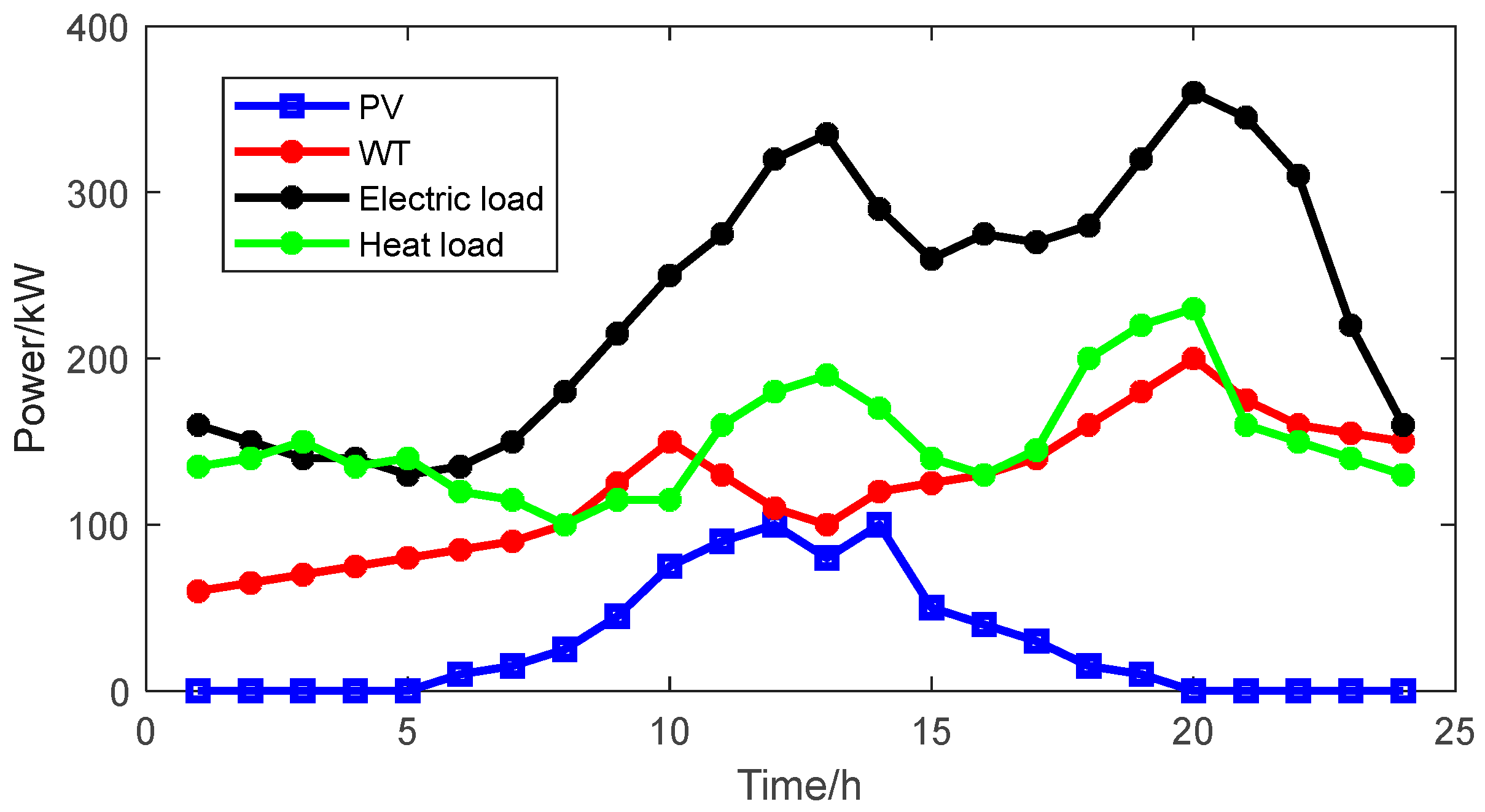
To verify the effectiveness of the proposed method, a classical integrated energy system (IES) consisting of PV, WT, MT, electrical energy storage batteries, and heat storage tanks is selected as the test system. The forecasted output power of the PV and WT, together with the forecasted electric and heat load profiles, is illustrated in Figure 3. All data were derived from the representativeness of the simulation scenarios. The technical parameters of each component are tabulated in

Table 1. Unit power and equipment parameters.

Type	Power/kW		Coefficient CNY/(kW·h)	CO2 Emission Cost Coefficient /g/(kW·h)	Conversion Coefficient of Carbon Emission Allowances/g/(kW·h)
	Minimum	Maximum
WT	0	$P_{t,\max }^{WT}$: Forecasted output	${\lambda }^{WT}$: 0.30	${\eta }_{WT}$: 76.6	${\gamma }_{WT}$: 43
PV	0	$P_{t,\max }^{PV}$: Forecasted output	${\lambda }^{PV}$: 0.35	${\eta }_{PV}$: 132.5	${\gamma }_{PV}$: 78
Microgrid	0	$P_{t,\max }^{Net}$: 160	Time of Use	${\eta }_{NET}$: 1303	${\gamma }_{NET}$: 798
MT	0	$P_{t,\max }^{MT}$: 65	${\lambda }^{MT}$: 0.57	${\eta }_{MT}$: 129.37	${\gamma }_{MT}$: 97.14
GB	0	$P_{t,\max }^{GB}$: 160	${\lambda }^{GB}$: 0.26	${\eta }_{GB}$: 58.21	${\gamma }_{GB}$: 43.71
ESS	-	-	${\lambda }^{ESS}$: 0.5	${\eta }_{ESS}$: 91.30	-

and

Table 2. Parameters of the energy storage system.

Type	Parameters
Battery	Ecap, min /kW·h	Ecap, max /kW·h	Pex, min /kW	Pex, max /kW	SOC(0) /kW·h	Charging/discharging efficiency
	40	95	30	40	40	0.9/0.9
Heat storage tanks	Qcap, min /kW·h	Qcap, max /kW·h	Qex, min /kW	Qex, max /kW	SOC(0) /kW·h	Charging/discharging efficiency
	40	95	5	30	40	0.9/0.9

. Notably, the heat conversion efficiency of the MT is set to 0.83. The optimal problem of the proposed model is formulated as a Mixed-Integer Linear Programming (MILP) model and solved exactly using the CPLEX solver. The simulation platform is MATLAB 2022b, utilizing the YALMIP and CPLEX optimization toolboxes for modeling and optimal solution analysis. The key parameters of CPLEX are listed in

Table 3. The key parameters of CPLEX.

Parameter	MIP Gap	Time Limits
Value	1.0 × 10−4	600 s

.

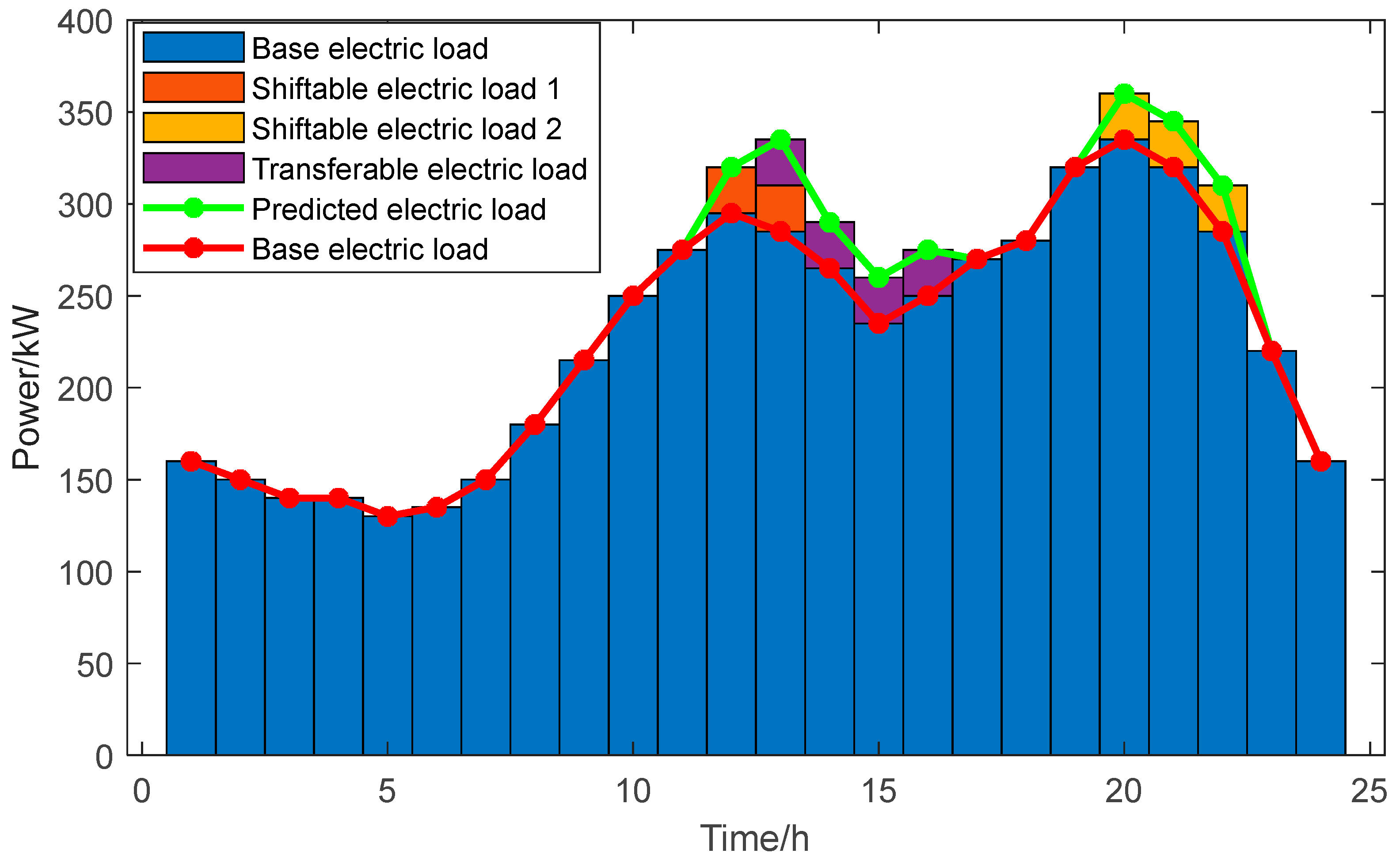
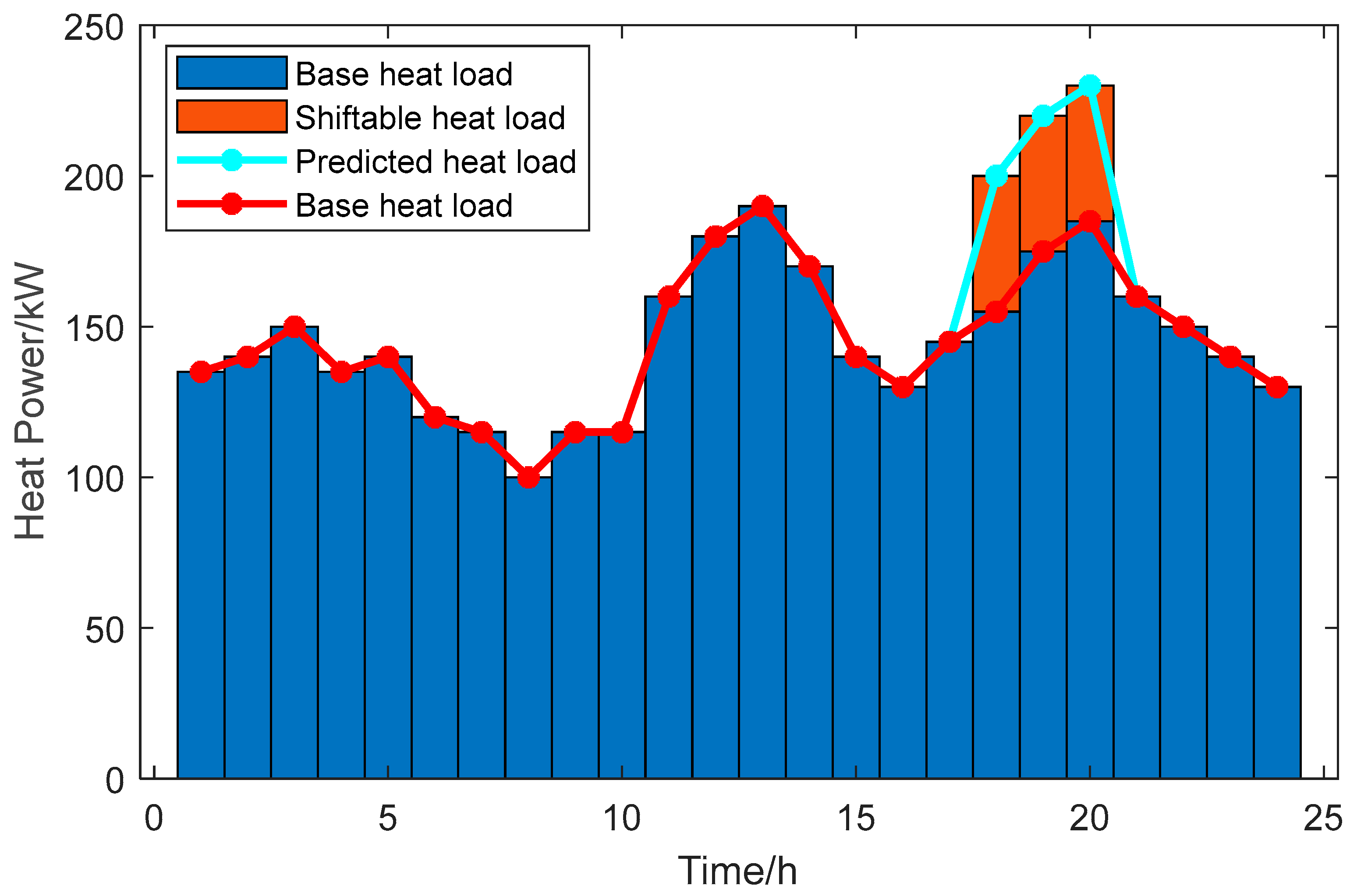
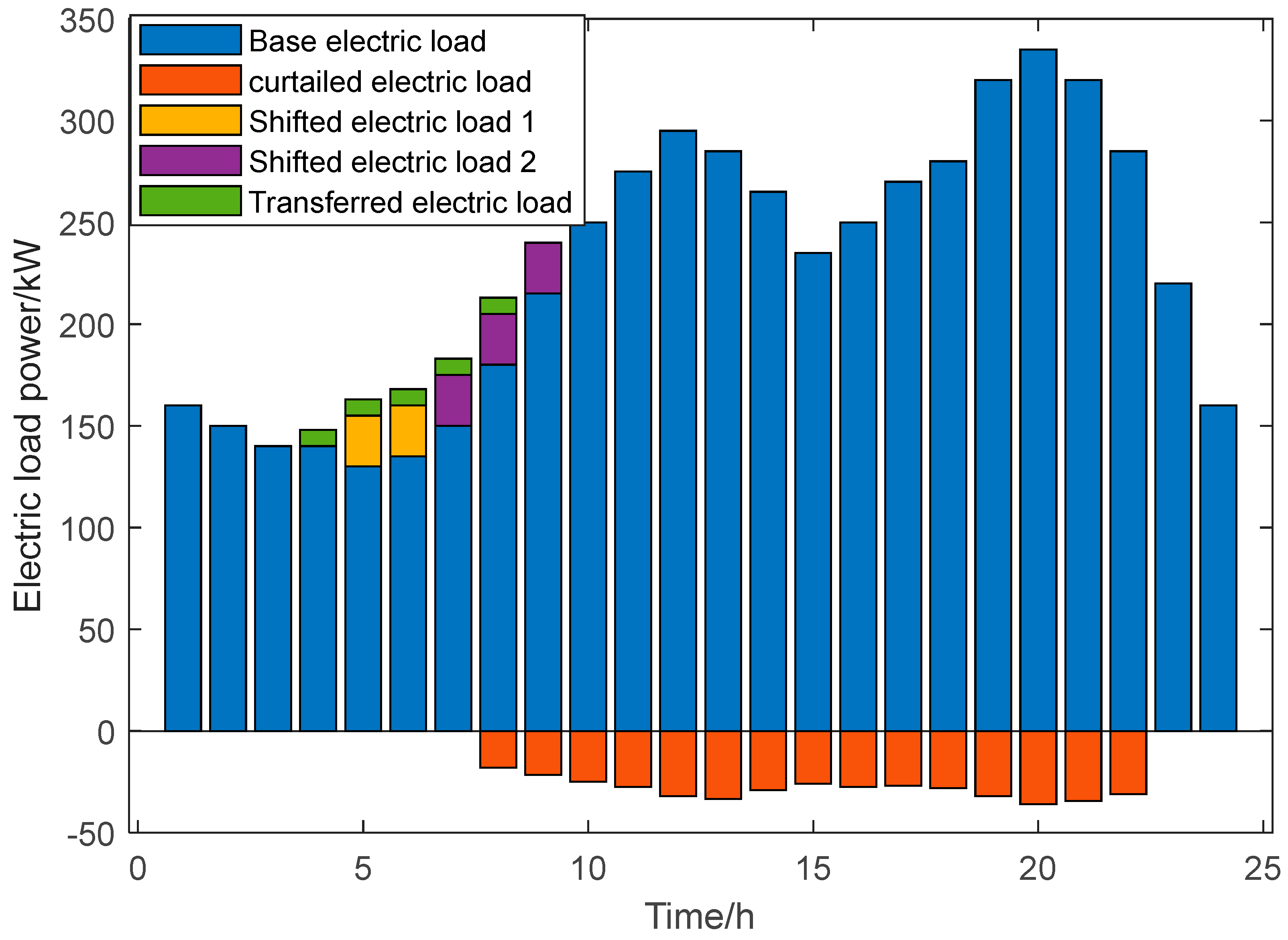
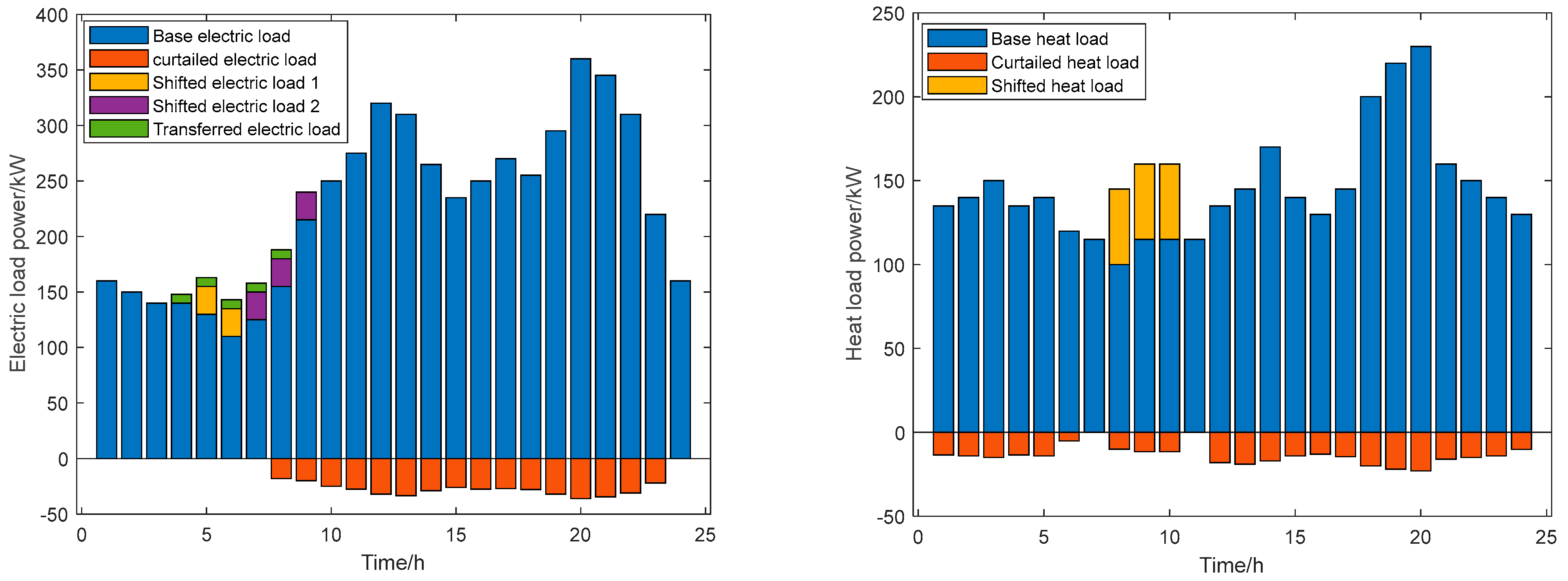
Figure 4 illustrates the distribution of predicted user-side electric loads, comprising the base electric load, two shiftable electric loads (designated as shiftable electric load 1 and shiftable electric load 2, respectively), and a transferable electric load. Correspondingly, Figure 5 presents the distribution of predicted user-side heat loads, comprising the base heat load and a shiftable heat load. The parameters of the flexible electric and heat loads prior to optimization are listed in

Table 4. Parameters of shiftable loads.

Type	Start Time	tD/h	$\left[{\mathit{t}}_{\mathit{s}\mathit{h}}^{-}, {\mathit{t}}_{\mathit{s}\mathit{h}}^{+}\right]$	${\mathit{\lambda }}_{\mathit{c}\mathit{o}\mathit{s}\mathit{t}}^{\mathit{s}\mathit{h}\mathit{i}\mathit{f}\mathit{t},\mathit{x}}$/CNY/(kW·h)
shiftable electric load 1	11:00	2	04:00~22:00	0.2
shiftable electric load 2	19:00	3	06:00~21:00	0.2
shiftable heat load 1	17:00	3	05:00~21:00	0.1

,

Table 5. Parameters of the transferable load.

Type	${\mathit{T}}_{\mathbf{min}}^{\mathit{t}\mathit{r}\mathit{a}\mathit{n},\mathit{x}}$/h	${\mathit{P}}_{\mathbf{min}}^{\mathit{t}\mathit{r}\mathit{a}\mathit{n},\mathit{x}}$/kW	${\mathit{P}}_{\mathbf{max}}^{\mathit{t}\mathit{r}\mathit{a}\mathit{n},\mathit{x}}$/kW	$\left[{\mathit{t}}_{\mathit{t}\mathit{r}}^{-},{\mathit{t}}_{\mathit{t}\mathit{r}}^{+}\right]$	${\mathit{\lambda }}_{\mathit{c}\mathit{o}\mathit{s}\mathit{t}}^{\mathit{t}\mathit{r}\mathit{a}\mathit{n},\mathit{x}}$/CNY/(kW·h)
transferable electric load 1	2	8	26.7	04:00~22:00	0.3

and

Table 6. Parameters of curtailable loads.

Type	${\mathit{\alpha }}_{\mathit{c}\mathit{u}\mathit{t}}^{\mathit{x}}$	${\mathit{\lambda }}_{\mathit{c}\mathit{o}\mathit{s}\mathit{t}}^{\mathit{c}\mathit{u}\mathit{t},\mathit{x}}$/CNY/(kW·h)
curtailable electric load	10%	0.4
curtailable heat load	10%	0.2

. It should be noted that heat loads that possess this transferable characteristic are rarely encountered in practice. Therefore, the transferable heat load is not tested in the experiment. In addition, it is stipulated that the maximum load curtailment ratio shall not exceed 10% of the predicted value.

5.1. Simulation Results Analysis

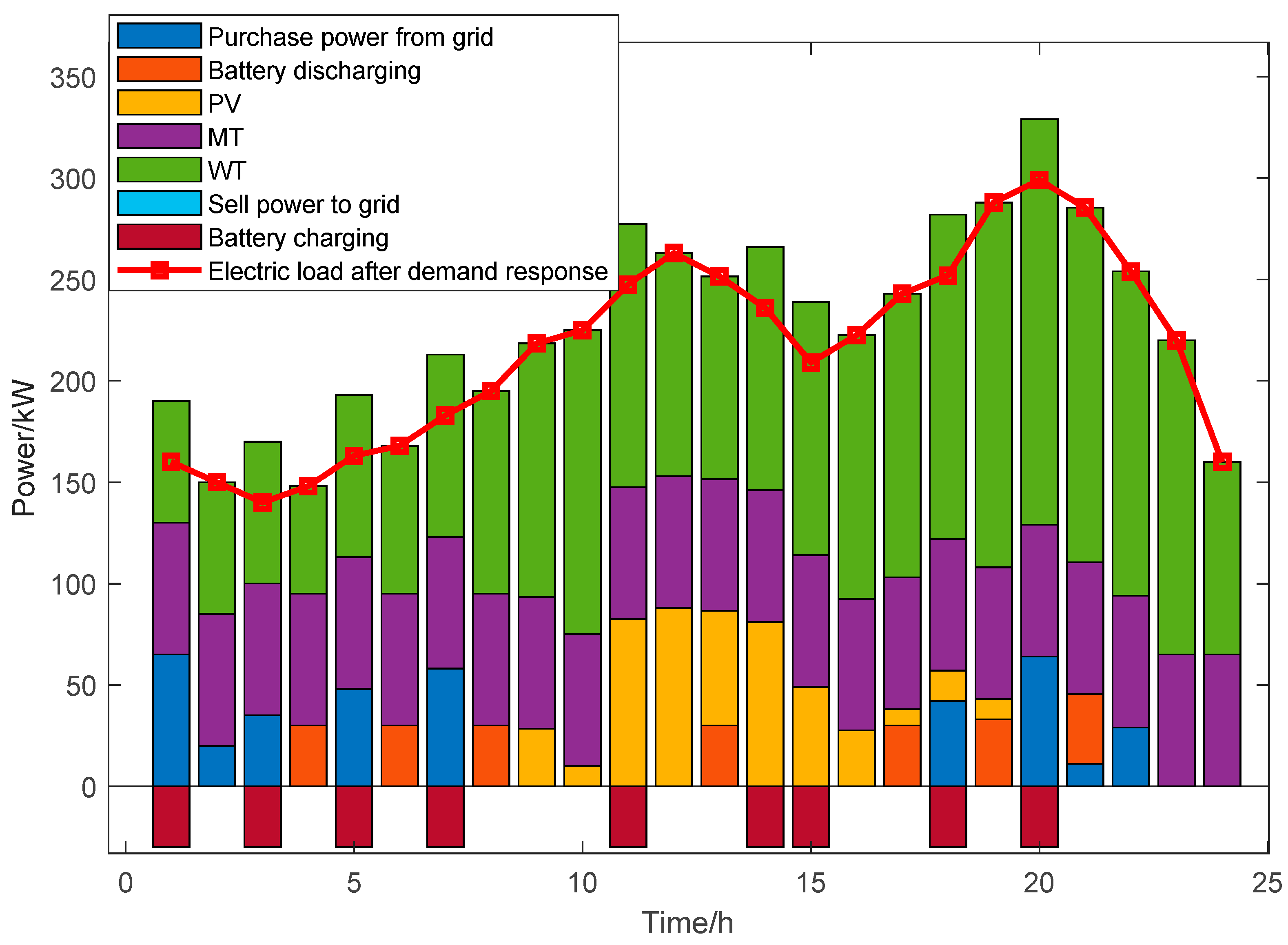
Figure 6 presents the collaborative optimization results of the IES with diverse flexible loads under the carbon trading mechanism. For the electric load, during the 00:00–06:00 period, the electricity price is in the valley period at 0.25 CNY/kW·h (as shown in Figure 7), while the operating cost of the WT is 0.30 CNY/kW·h, slightly higher than the grid purchasing price. Therefore, priority is given to power supply from the power grid and WT. As the MT operates in the “heat-following” mode, it generates a certain amount of electricity, and the surplus energy is used to charge the energy storage batteries. During the 09:00–15:00 and 18:00–21:00 periods, distributed energy resources are abundant, and the grid purchasing cost is high; thus, wind and solar resources are fully utilized for power supply. Meanwhile, the energy stored in the batteries is discharged during peak load periods (e.g., 19:00–21:00) to meet the high demand.

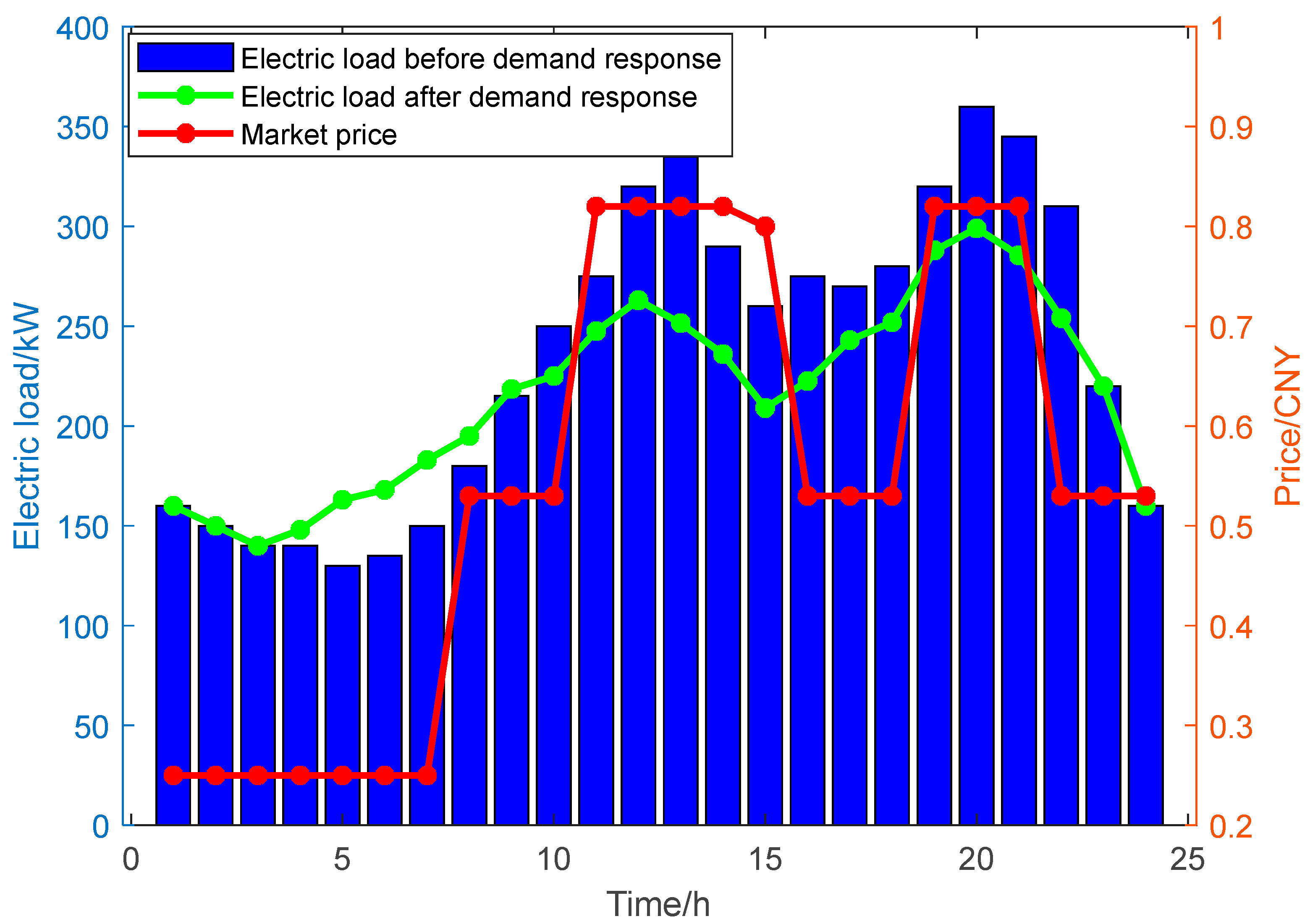
Figure 7 shows the electric load curves before and after demand response. It can be observed that electricity prices are relatively high during the periods of 10:00–14:00 and 18:00–20:00. Consequently, under the carbon trading mechanism and following user-side demand response (including load shifting, transferring, and curtailment), the optimized results are presented in Figure 8. Specifically, shiftable electric load 1 is shifted to 04:00–06:00, shiftable electric load 2 to 06:00–9:00, and the transferable load to 03:00–08:00. All these time windows fall within the low electricity price range, which contributes to reducing user costs. Regarding curtailable load, as indicated by the red bar in Figure 8, curtailment is concentrated between 07:00 and 22:00, a period when electricity prices are relatively high, and peak power demand occurs. The demand response of these flexible loads makes the load distribution smoother compared to that before demand response, as shown by the green curve in Figure 7. This indicates that user-side demand response can reduce the overall operating cost of the IES and achieve the effect of peak shaving and valley filling, to a certain extent.

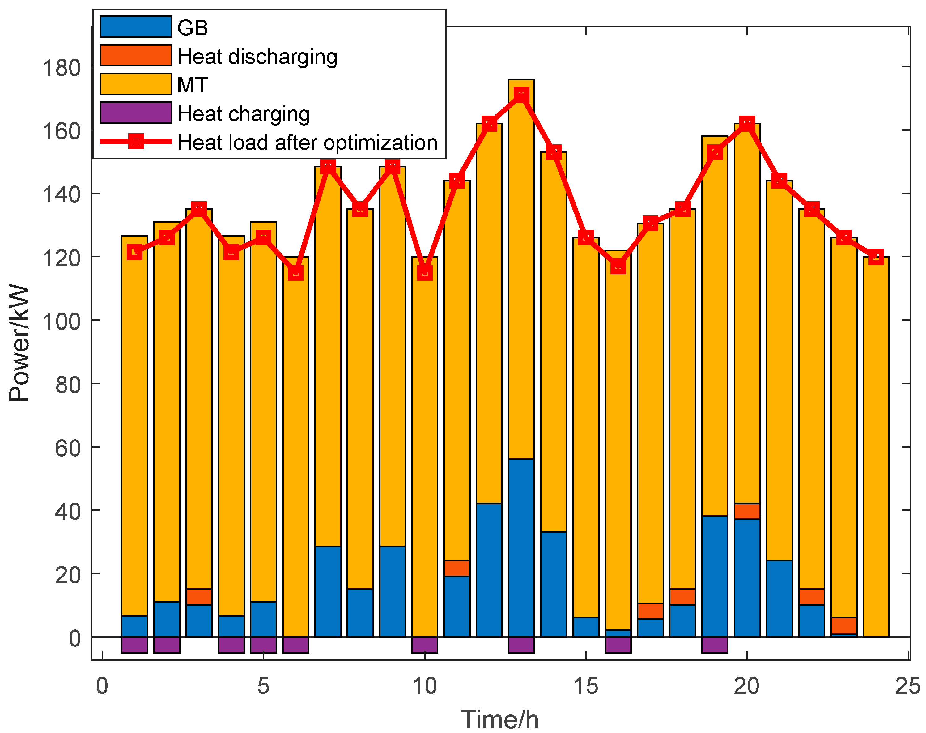
For the heat load, the collaborative optimization results of the IES are shown in Figure 9. It can be observed that the heat output is primarily provided by the MT, in coordination with supplementary supply from the GB and the heat storage tank. Combining the analysis of Figure 6 and Figure 9, the MT operates almost at full capacity, compensating for both electricity and heat deficits. During the 00:00–06:00 period, the combined electrical and heat output of the MT minimizes grid power purchases; the surplus electrical energy is absorbed by the batteries, thereby reducing the power dispatch cost during this period. During the 08:00–24:00 period, specifically at 00:00–06:00, 10:00, 13:00, 16:00, and 19:00, the GB charges the heat storage tank. When the heat load reaches peak periods, such as at 20:00 and 22:00–23:00, the heat storage tank discharges heat to meet the increased demand.

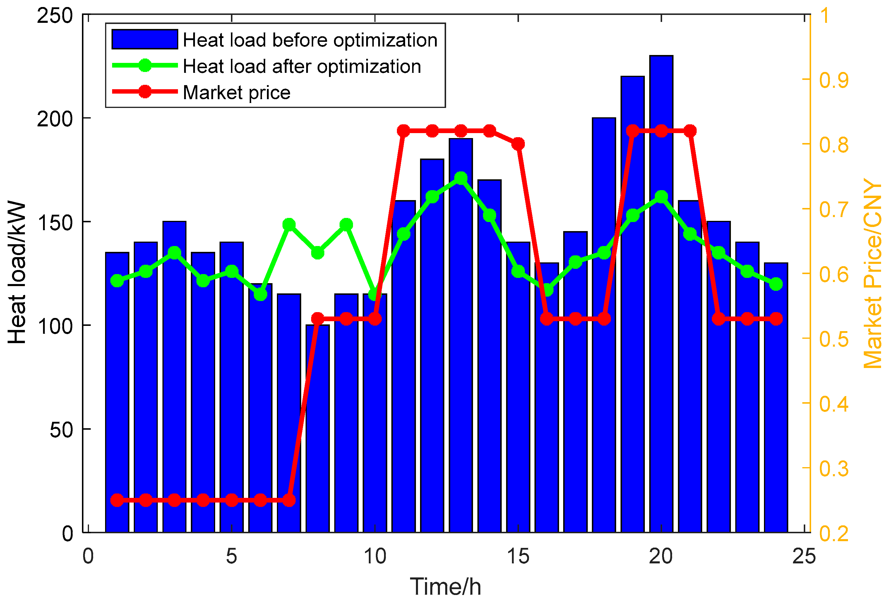
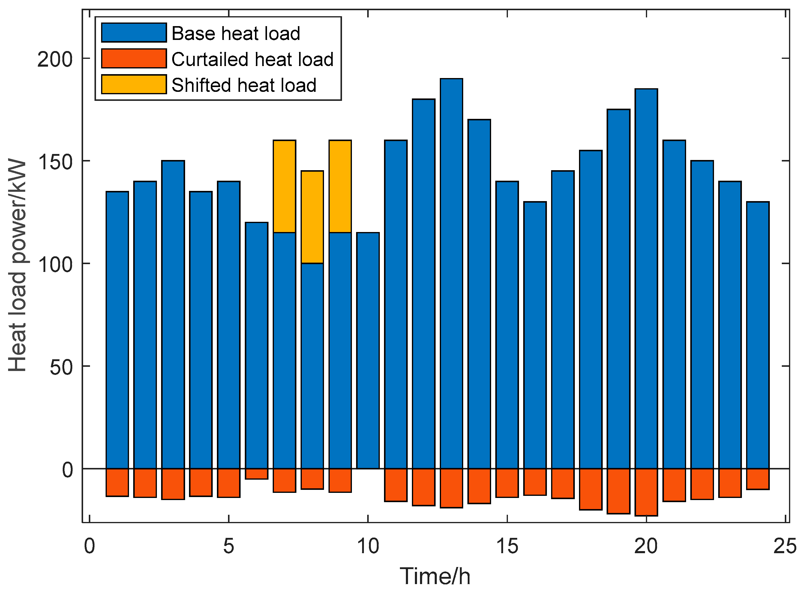
Figure 10 presents the heat load curves before and after demand response. Heat prices are relatively high during the periods of 10:00–15:00 and 18:00–21:00. Under the carbon trading mechanism and following user-side demand response (including heat load shifting and curtailment), the results are shown in Figure 11. Specifically, Shiftable heat load 1 is shifted to 06:00–09:00, a time window with lower heat prices, which helps reduce user costs. Additionally, as indicated by the green curve in Figure 10, the demand response of flexible heat loads results in a smoother heat load profile compared to the pre-demand response scenario. This further confirms that user-side demand response not only reduces the overall operating cost of the IES but also plays a significant role in peak shaving and valley filling for heat loads.

5.2. Comparison

5.2.1. Benefits of Considering Demand Response

To further illustrate the economic benefits of considering demand response under the carbon trading mechanism (the parameters in

Table 7. Parameters of the carbon trading mechanism.

Parameter	L/g	${\mathit{\lambda }}_{\mathit{b}\mathit{a}\mathit{s}\mathit{e}}^{\mathit{C}{\mathit{O}}_2}$/(CNY/g)	K	${\mathit{\lambda }}^{\mathit{g}\mathit{r}\mathit{e}\mathit{e}\mathit{n}}$/(CNY/g)
Value	120,000	0.00015	5	0.21

),

Table 8. Cost analysis.

Case	${\mathit{f}}_{\mathit{B}\mathit{u}\mathit{y}}$/CNY	${\mathit{f}}_{\mathit{C}{\mathit{O}}_2}$/CNY	${\mathit{f}}_{\mathit{F}\mathit{u}\mathit{e}\mathit{l}}$/CNY	${\mathit{f}}_{\mathit{O}\mathit{P}}$/CNY	${\mathit{f}}_{\mathit{P}\mathit{u}\mathit{n}}$/CNY	${\mathit{f}}_{\mathit{g}\mathit{r}\mathit{e}\mathit{e}\mathit{n}}$/CNY	f/CNY
Case 1	895.04	316.49	1066.62	2078.04	0	647.12	3709.06
Case 2	155.78	80.37	997.22	2092.05	289.87	693.42	2921.87

presents the results of the proposed model under two scenarios: Case 1 (without flexible load demand response) and Case 2 (with flexible load demand response, i.e., the proposed method). It can be observed that the total cost in Case 2 is lower than that of Case 1. Specifically, flexible load demand response enables the transfer of part of the load from high-price periods to low-price periods, thereby reducing the cost of power transactions with the main grid. Secondly, with the incorporation of demand response, the coordinated operation of various energy units leads to a significant reduction in the cost of carbon trading $f_{C{O}_2}$. In addition, although the cost of $f_{Pun}$ in Case 1 is zero, the final total cost of Case 1 is still 787.19 CNY higher than that of Case 2. This indicates that the economic advantages brought by demand response (e.g., reduced grid transaction costs and optimized unit operation efficiency) outweigh the potential carbon trading expenses, verifying the economic feasibility and superiority of the proposed model.

5.2.2. Benefits of Considering the Green Certificate

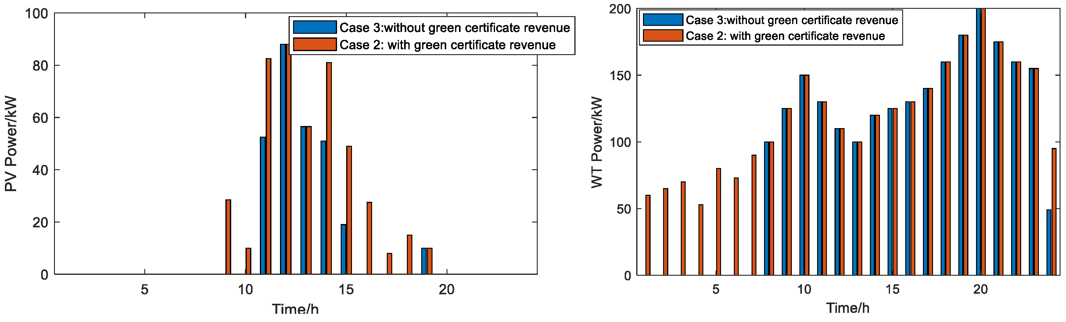
To verify the validity of the green certificate revenue, denoted as $f_{green}$, which is subtracted from total costs, three cases were established. Case 2 represents the proposed method, Case 3 removes the green certificate revenue, and Case 4 involves the green certificate revenue with changing the sign. The respective objective functions are presented as follows:

$$\begin{array}{ll}\mathrm{Case} 2:& \min f=f_{Buy}+f_{Fuel}+f_{C{O}_2}+f_{OP}+f_{Pun}-f_{green}\\ \mathrm{Case} 3:& \min f=f_{Buy}+f_{Fuel}+f_{C{O}_2}+f_{OP}+f_{Pun}\\ \mathrm{Case} 4:& \min f=f_{Buy}+f_{Fuel}+f_{C{O}_2}+f_{OP}+f_{Pun}+f_{green}\end{array}$$

Figure 12 illustrates the distribution of wind and PV energy usage. In terms of PV distribution, the PV energy used in Case 3 and Case 4 is significantly lower than that in Case 2 during 9:00–11:00 and 14:00–19:00. Additionally, from the perspective of wind energy, there is basically no wind energy utilization in Case 3 and Case 4 from 0:00 to 8:00. This demonstrates that by subtracting the green certificate revenue from the total costs, the proposed method can improve the utilization of renewable energy sources such as PV and wind power.

Table 9. Cost analysis by considering the green certificate.

Case	${\mathit{f}}_{\mathit{B}\mathit{u}\mathit{y}}$/CNY	${\mathit{f}}_{\mathit{C}{\mathit{O}}_2}$/CNY	${\mathit{f}}_{\mathit{F}\mathit{u}\mathit{e}\mathit{l}}$/CNY	${\mathit{f}}_{\mathit{O}\mathit{P}}$/CNY	${\mathit{f}}_{\mathit{P}\mathit{u}\mathit{n}}$/CNY	${\mathit{f}}_{\mathit{g}\mathit{r}\mathit{e}\mathit{e}\mathit{n}}$/CNY	f/CNY
Case 2	155.78	80.37	997.22	2092.05	289.87	693.42	2921.87
Case 3	895.04	316.49	1066.62	2078.04	0	647.12	3709.06
Case 4	915.59	997.22	305.60	1133.00	345.26	322.03	4018.70

lists the cost of three cases. It can be seen that the energy trading costs $f_{Buy}$ and carbon trading costs $f_{C{O}_2}$ in the proposed method (Case 2) are significantly lower than those of Case 3 and Case 4. Although the fuel costs $f_{Fuel}$ and operation and maintenance costs $f_{OP}$ decreased in Case 4, the final cost is higher than that of the proposed method due to the $f_{Buy}$ and $f_{C{O}_2}$. This indicates that the proposed method can reduce carbon trading costs and provide support for the low-carbon target.

5.3. Sensitivity Analysis of Parameters in the Flexible Load

In the proposed method, this compensation cost $f_{Pun}$ is divided into three parts: shiftable, transferable, and curtailable loads, which contains several parameters. To evaluate their impact on the overall objective function, an optimal search for the parameters of the flexible load was performed using the Harris Hawks Optimization (HHO) method [27] with a population size of 30. The upper and lower limits of the parameters are listed in the ‘Search Range’ column of

Table 10. Parameters setting for the flexible load.

Parameter	Search Range	Optimal Value
${\lambda }_{cost}^{shift,e}$/(CNY/kW·h)	[0.1, 2]	2
${\lambda }_{cost}^{shift,h}$/(CNY/kW·h)	[0.1, 2]	0.1
${\lambda }_{cost}^{tran,e}$/(CNY/kW·h)	[0.1, 2]	0.1
${\lambda }_{cost}^{tran,h}$/(CNY/kW·h)	[0.1, 2]	--
${\lambda }_{cost}^{cut,e}$/(CNY/kW·h)	[0.1, 2]	0.1
${\lambda }_{cost}^{cut,h}$/(CNY/kW·h)	[0.1, 2]	1.9272
$P_{\min }^{tran,e}$/kW	[8.0, 26.7]	17.4528
${\alpha }_{cut}^e$	[10%, 50%]	50%
${\alpha }_{cut}^h$	[10%, 50%]	50%

. The optimal results obtained through the HHO search are presented in the ‘Optimal Value’ column.

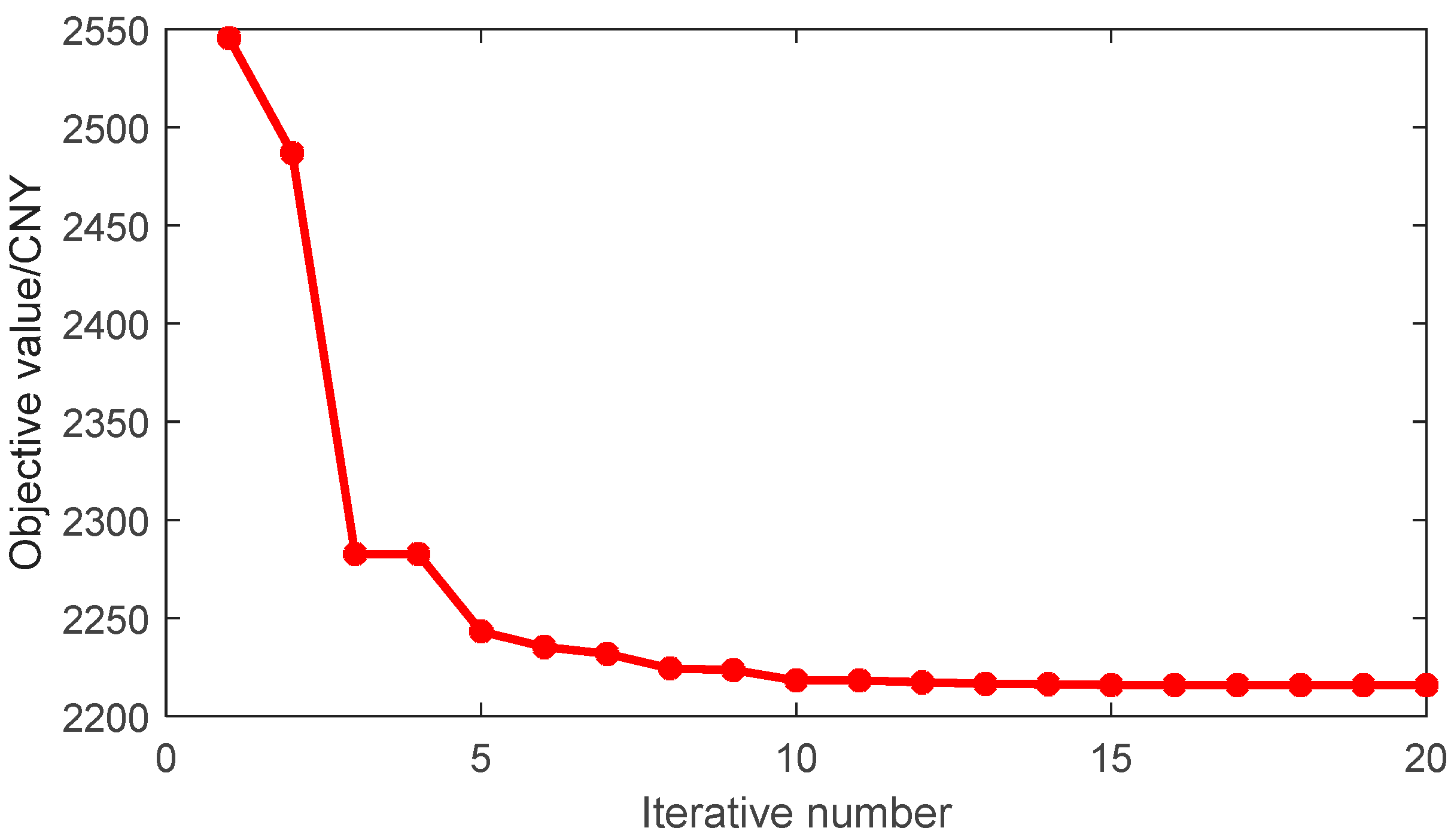
Figure 13 illustrates the objective function curve throughout the iteration process. It can be observed that a superior objective value is ultimately achieved as the parameters are optimized. Compared with the objective value obtained by the baseline method (using default parameters), this optimal parameter setting strategy yields better economic benefits, as shown in

Table 11. Cost analysis by considering the flexible load demand with the optimal parameter.

	${\mathit{f}}_{\mathit{B}\mathit{u}\mathit{y}}$/CNY	${\mathit{f}}_{\mathit{C}{\mathit{O}}_2}$/CNY	${\mathit{f}}_{\mathit{F}\mathit{u}\mathit{e}\mathit{l}}$/CNY	${\mathit{f}}_{\mathit{O}\mathit{P}}$/CNY	${\mathit{f}}_{\mathit{P}\mathit{u}\mathit{n}}$/CNY	${\mathit{f}}_{\mathit{g}\mathit{r}\mathit{e}\mathit{e}\mathit{n}}$/CNY	f/CNY
value	−422.24	104.87	1084.88	1305.23	555.73	412.60	2215.87

. This demonstrates that the participation of flexible load in demand response, combined with reasonable parameter settings, can effectively improve the economic benefits of the integrated energy system. Nevertheless, as it is based on the known flexible loads and load forecasting, adopting fixed values of parameters might be more practical for actual scenarios.

5.4. Coupling Effects Between the Start Time of the Flexible Load and Its Demand Response

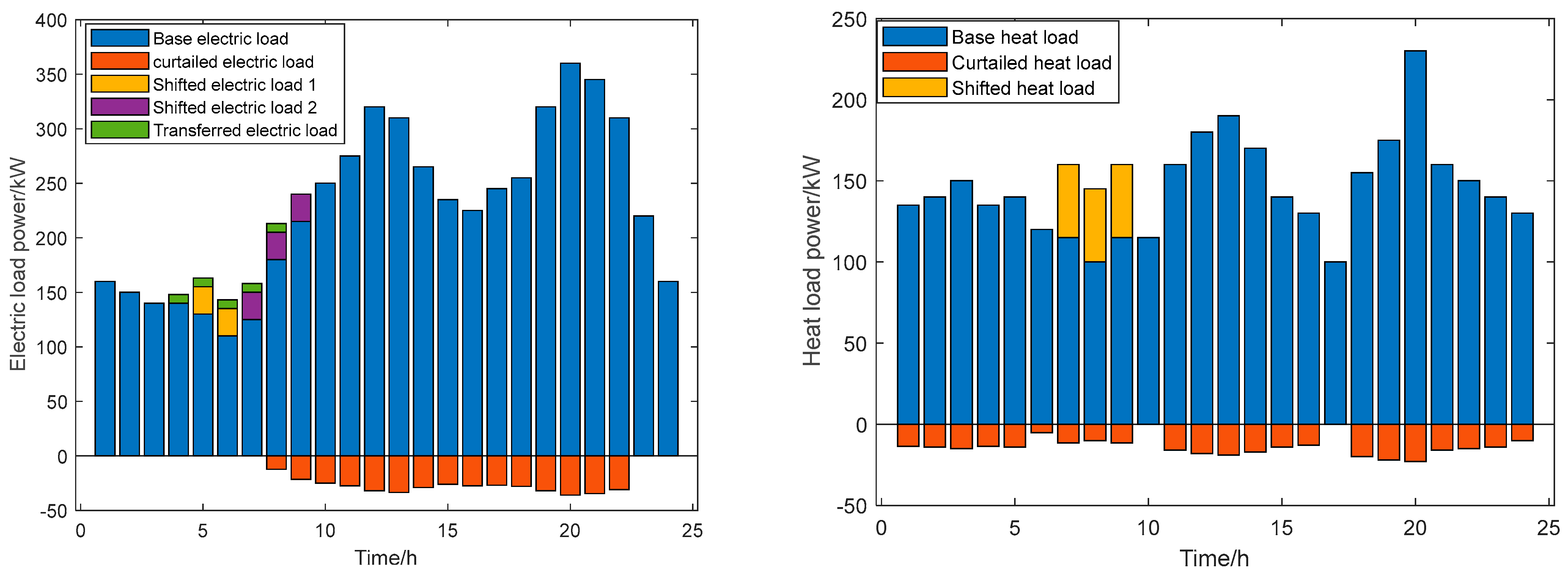
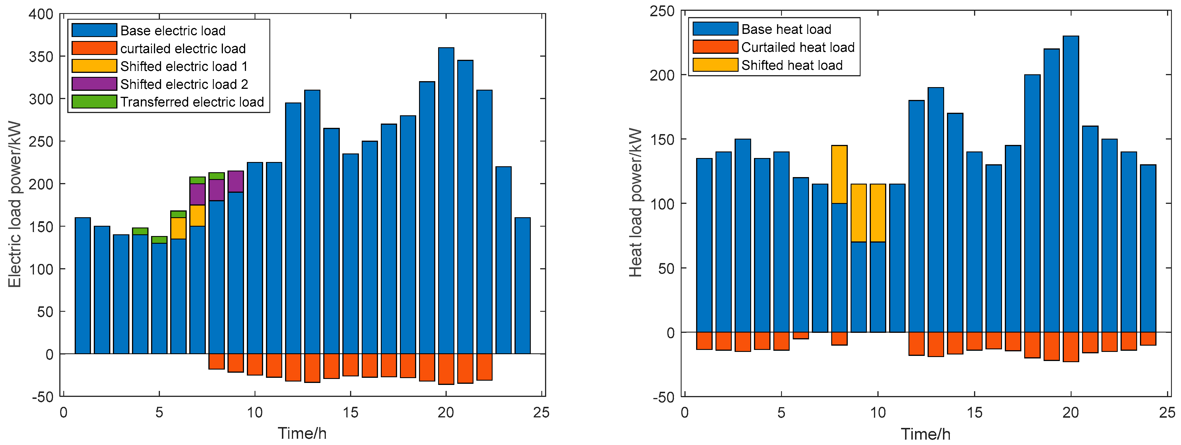
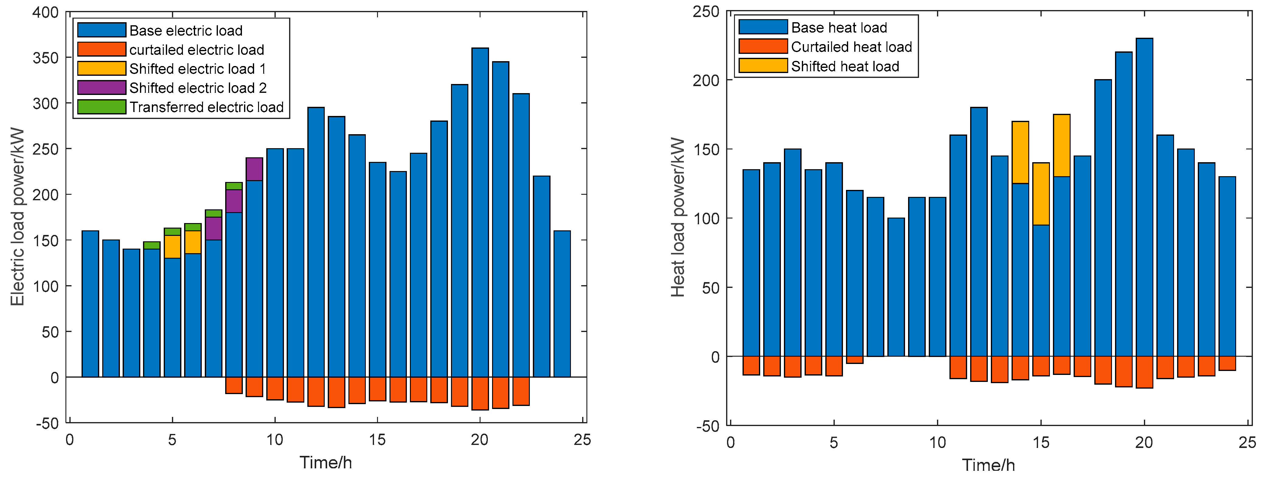
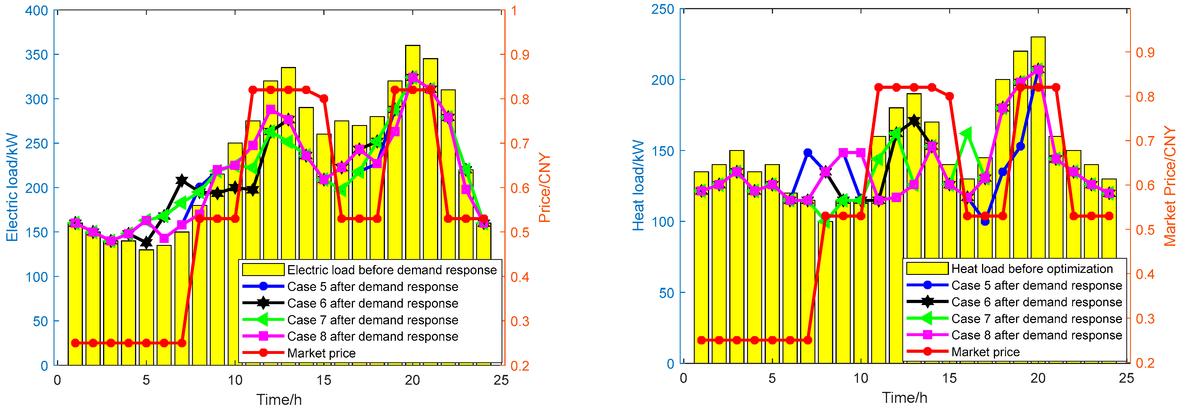
To further discuss the shiftable loads with specific start times, four cases with different start times of flexible loads were analyzed, as shown in

Table 12. Parameters of shiftable loads with different starting times.

Type	Start Time (Case 5)	Start Time (Case 6)	Start Time (Case 7)	Start Time (Case 8)	tD/h	$\left[{\mathit{t}}_{\mathit{s}\mathit{h}}^{-}, {\mathit{t}}_{\mathit{s}\mathit{h}}^{+}\right]$	${\mathit{\lambda }}_{\mathit{c}\mathit{o}\mathit{s}\mathit{t}}^{\mathit{s}\mathit{h}\mathit{i}\mathit{f}\mathit{t},\mathit{x}}$/CNY/(kW·h)
shiftable electric load 1	5:00	10:00	15:00	17:00	2	04:00~22:00	0.2
shiftable electric load 2	15:00	8:00	10:00	5:00	3	06:00~21:00	0.2
shiftable heat load 1	16:00	8:00	12:00	10:00	3	05:00~21:00	0.1

. The results are presented in Figure 14, Figure 15, Figure 16 and Figure 17. From the results, the start times for shiftable electric load 1 in Case 5, Case 7, and Case 8 occur at 04:00, while Case 6 occurs at 05:00; the start times for shiftable electric load 2 are all at 06:00. These time windows correspond to periods of relatively low electricity prices. For shiftable heat load 1, the start time in Case 5 occurs at 06:00, Case 6 and Case 8 at 07:00, and Case 7 at 13:00. Due to the changes in the start times of shiftable loads, the transferable loads and curtailable loads also underwent corresponding adjustments to enable the IES to coordinate various resources. Figure 18 presents the load curves after flexible load demand response. Compared with the original predicted load, these results reflect the effect of peak shaving and valley filling to a certain extent.

Additionally,

Table 13. Cost analysis by considering the shiftable load with different starting times.

Case	${\mathit{f}}_{\mathit{B}\mathit{u}\mathit{y}}$/CNY	${\mathit{f}}_{\mathit{C}{\mathit{O}}_2}$/CNY	${\mathit{f}}_{\mathit{F}\mathit{u}\mathit{e}\mathit{l}}$/CNY	${\mathit{f}}_{\mathit{O}\mathit{P}}$/CNY	${\mathit{f}}_{\mathit{P}\mathit{u}\mathit{n}}$/CNY	${\mathit{f}}_{\mathit{g}\mathit{r}\mathit{e}\mathit{e}\mathit{n}}$	f/CNY
Case 5	185.43	82.98	1000.17	2106.00	284.70	697.32	2961.96
Case 6	211.28	89.57	1007.17	2036.98	282.13	677.36	2949.77
Case 7	191.66	88.21	1004.87	2069.30	283.31	686.78	2950.57
Case 8	180.73	80.39	1001.29	2083.53	294.89	689.01	2951.82

lists the cost components within the objective function. The variation in the start times of shiftable loads did not have a significant impact on the final operating costs. This indicates that through synergistic interaction with the carbon trading mechanism and the flexible adjustment of flexible loads, the linkage of multi-energy equipment, such as energy storage, heat, and electricity, can be realized. This enhances the energy system’s coordination capabilities for various resources, improves the flexibility of resource supply and demand, and reduces overall system carbon emissions, thereby balancing economic benefits with low-carbon objectives.

6. Conclusions

This paper establishes a flexible load model for an IES and proposes a collaborative optimization model tailored to the carbon trading mechanism. Specifically, a joint optimal scheduling model for system supply and demand is further established to minimize daily costs. Case study results demonstrate that the curtailable loads can achieve peak load shaving, while shiftable and transferable loads play a role in load peak shifting. Through comparative analysis of the IES operating costs with and without flexible load participation, it is verified that the participation of flexible loads not only optimizes the profiles of electric and heat load curves but also significantly reduces the total system operating cost, thereby achieving the goal of economic dispatch for the IES. Furthermore, the flexible load model takes into account user electricity consumption characteristics and satisfies user comfort requirements, demonstrating good feasibility for engineering applications. In future research, degradation-related costs associated with energy storage systems will be refined, and the compensation cost mechanism for demand response will be further enhanced. Additionally, the optimal method for the carbon allowance allocation will be designed, and the scope of application will be expanded to extend the flexible load model to interconnected multi-integrated energy systems (multi-IESs), aiming to achieve more comprehensive optimal operation of regional integrated energy networks.