Capacity Optimization and Rolling Scheduling of Offshore Multi-Energy Coupling Systems

Abstract

Increasing penetration of offshore renewable energy has highlighted the challenges posed by strong intermittency, output uncertainty, and insufficient utilization of marine energy resources. To address these issues, this study investigates an offshore multi-energy coupling system integrating wind, photovoltaic, tidal, and wave energy with flexible loads such as seawater desalination and hydrogen production. A coordinated two-stage optimization framework is proposed. In the planning stage, a joint operation–planning capacity configuration model is formulated to minimize the annualized system cost while determining the optimal sizes of generation units and energy storage. In the operational stage, a multi-time-scale rolling scheduling model combining day-ahead and intra-day optimization is developed to dynamically mitigate renewable output fluctuations and enhance system flexibility. Case studies verify that the proposed framework significantly improves renewable energy utilization, reducing the curtailment rate to 0.7%, while achieving stable and cost-effective operation. The results demonstrate the effectiveness of coordinated planning and rolling scheduling for future offshore integrated energy systems.

1. Introduction

Driven by global decarbonization goals, offshore renewable energy systems are gaining strategic importance due to their large resource potential and suitability for large-scale clean-energy deployment. Wind, photovoltaic, tidal current, and wave resources exhibit strong complementarity but also pronounced intermittency, stochasticity, and forecast uncertainty [1,2,3,4]. These characteristics significantly constrain the operational stability of single-source systems and have motivated growing interest in integrated multi-energy coupling architectures that can exploit cross-resource complementarities [5,6,7].

To address the limitations of standalone generation units, offshore energy development is increasingly shifting toward unified, multi-energy integrated configurations [8,9]. Hybrid systems combining wind, wave, tidal current, and offshore photovoltaic generation have shown significant potential to enhance energy utilization and improve robustness under dynamic marine conditions [10,11]. These systems further extend into diversified application scenarios—including offshore agriculture, renewable-powered offshore platforms, and multi-energy service clusters [12,13]. However, despite these advancements, challenges persist in the depth of energy integration, platform compactness, real-time control coordination, operational resilience under fluctuating sea states, and economic optimality [14,15]. These gaps highlight the need for a joint framework capable of simultaneously addressing system-level configuration and time-sensitive operational decision-making.

Existing research on offshore multi-energy systems covers capacity planning, economic optimization, and scheduling coordination, often formulated as multi-objective optimization problems balancing economy, carbon reduction, and reliability [16,17]. Day-ahead scheduling models focus on long-horizon economic operation [18,19,20], whereas intra-day models emphasize high-resolution adaptation to rapid fluctuations [21,22]. Emerging hybrid storage frameworks incorporating electrolysis, compressed-air storage, and battery systems improve operational flexibility [23,24,25,26]. Nevertheless, many existing methods rely on static time-scale assumptions or isolated scheduling layers, limiting their ability to handle forecast errors and sudden renewable variability [27,28]. Moreover, multi-energy microgrids and carbon emission are the key point of the application of renewable variability [29,30].

This study addresses these limitations by proposing a coordinated two-level operation–planning optimization framework. At the planning level, the model identifies an optimal capacity mix that balances investment cost and operational adaptability while capturing multi-energy complementarities. At the operational level, a rolling optimization strategy integrates day-ahead and intra-day scheduling, enabling real-time adjustments based on updated renewable forecasts. Leveraging the reduced prediction error at shorter time scales, a multi-time-scale scheduling scheme is established to enhance renewable-energy absorption and system stability. The proposed framework provides a unified pathway for achieving economic efficiency and dynamic operational robustness in offshore multi-energy coupling systems.

The novelty of our proposed framework for optimizing renewable energy systems with seasonal considerations lies in a combination of multiple aspects, rather than being solely attributed to a single element. Firstly, the integration of the four offshore resources is indeed a significant innovative point. Traditional offshore energy systems often focus on a single or a limited number of energy sources. Secondly, the coupling of flexible loads also contributes to the novelty. Flexible loads, such as energy storage systems and demand—response are seamlessly integrated into our framework. This allows for dynamic adjustment of energy consumption according to the real—time availability of offshore renewable energy. Lastly, the improved Particle Swarm Optimization (PSO) mechanism plays a vital role. The standard PSO algorithm has certain limitations in dealing with complex multi—objective optimization problems in the context of offshore energy systems.

2. Offshore Multi-Energy Integrated Coupling System

2.1. Multi-Energy Coupling System Architecture

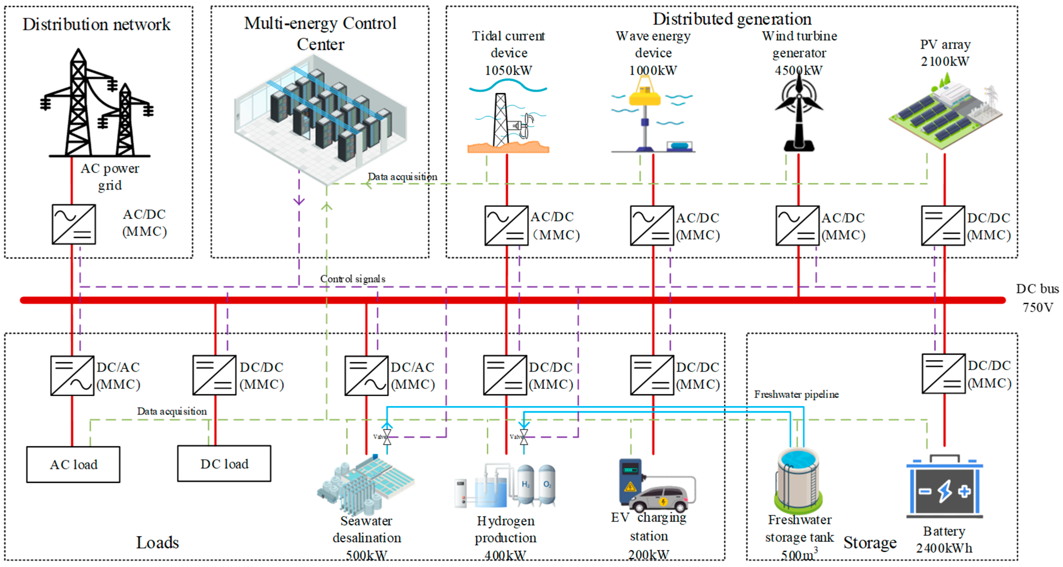
This study takes marine energy development as the starting point and establishes a multi-energy coupling direct current (DC) microgrid system incorporating renewable energy sources such as wind, tidal current, and wave energy, together with energy-consuming flexible loads including seawater desalination and hydrogen production. The structural configuration of the proposed multi-energy coupling DC microgrid system is illustrated in Figure 1.

In Figure 1, a single DC bus operating at a voltage level of 750 V is adopted to supply the multi-energy coupling DC microgrid system. Distributed energy sources—including tidal current energy devices, wave energy converters, wind turbine generators, and photovoltaic arrays—together with DC loads such as hydrogen production units and EV charging stations, Alternating current (AC) loads such as seawater desalination facilities, and energy storage devices such as batteries, are all connected to the DC bus via power electronic converters. The rectifier is used to convert AC into direct current DC. The inverter is employed to convert direct current DC into alternating current AC. The DC bus is interfaced with the AC distribution network through a bidirectional AC/DC modular multilevel converter to enable power exchange. A multi-energy complementary control center collects operational states of all distributed generation units, loads, and energy storage systems through a data acquisition bus, and dispatches control signals to the respective power electronic converters and freshwater delivery valves directly connected to the DC bus. Desalination meets the corresponding power load demand, while energy storage provides regulatory functions for the DC microgrid.

2.2. Models of Distributed Energy Generation Units

2.2.1. Wind Turbine Generation Model

The output power of the wind turbine can be expressed as follows:

$$\begin{array}{c}{P}_{WT}=\left\{\begin{array}{ll}0,\hfill & v<v_{in}\hfill \\ P_{W{T}_{rat}}({\displaystyle \frac{v-v_{in}}{v_{out}-v_{in}}}),\hfill & v_{in}\le v<v_{rat}\hfill \\ P_{W{T}_{rat}},\hfill & v_{rat}\le v<v_{out}\hfill \\ 0,\hfill & v\ge v_{out}\hfill \end{array}\right.\end{array}$$

(1)

where $P_{WT}$ is the output power of the wind turbine, $P_{WTrat}$ is the rated power of the wind turbine, $v$ denotes the wind speed, $v_{in}$ denotes the cut-in wind speed, $v_{out}$ denotes the cut-out wind speed, and $v_{rat}$ denotes the rated wind speed. When the wind speed is lower than $v_{in}$ or higher than $v_{out}$, the wind turbine shuts down. When the wind speed lies between $v_{in}$ and $v_{rat}$, the output power is a function of wind speed. When the wind speed lies between $v_{rat}$ and $v_{out}$, the wind turbine produces the rated power $P_{WTrat}$.

2.2.2. Photovoltaic Cell Model

The output power of the photovoltaic cell can be expressed as follows:

$$\begin{array}{c}{P}_{PV}={\alpha }_{PV}{S}_{PV}{\varphi }_t\end{array}$$

(2)

where $P_{PV}$ denotes the output power of the photovoltaic cell, ${\alpha }_{PV}$ denotes the power generation efficiency of the photovoltaic cell under maximum power point tracking (MPPT), $S_{PV}$ represents the total surface area of the PV panel, and ${\varphi }_t$ denotes the solar irradiance at time $t$.

2.2.3. Tidal Current Energy Generation Model

Since tidal current energy is more continuous and stable compared with wind energy, the output of a tidal current energy generator exhibits less variability than that of a wind turbine. In general, the water flow speed is insufficient to cause shutdown of the tidal current generator, and the cut-out flow speed is therefore not considered. Its output power can be expressed as follows:

$$P_{\mathrm{tidal}}(t)=\left\{\begin{array}{ll}{\left({\displaystyle \frac{v_{\mathrm{tidal}}(t)-v_{ci}^{\mathrm{tidal}}}{v_r^{\mathrm{tidal}}-v_{ci}^{\mathrm{tidal}}}}\right)}^3{P}_r^{\mathrm{tidal}},\hfill & v_{ci}^{\mathrm{tidal}}\le v_{\mathrm{tidal}}(t)\le v_r^{\mathrm{tidal}}\hfill \\ P_r^{\mathrm{tidal}},\hfill & v_{\mathrm{tidal}}(t)>v_r^{\mathrm{tidal}}\hfill \\ 0,\hfill & v_{\mathrm{tidal}}(t)<v_{ci}^{\mathrm{tidal}}\hfill \end{array}\right.$$

(3)

where $v_{\mathrm{tidal}}(t)$ denotes the tidal current velocity and represents the actual seawater flow speed at time $t$; $v_{ci}^{\mathrm{tidal}}$ denotes the cut-in flow speed; $v_r^{\mathrm{tidal}}$ denotes the rated flow speed; $P_r^{\mathrm{tidal}}$ denotes the rated power; and $P_{\mathrm{tidal}}(t)$ denotes the real-time output power.

2.2.4. Wave Energy Conversion Model

Based on its operating principle, the power output of a wave energy converter (WEC) can be divided into two processes: energy release and energy storage. During the energy-release process, the accumulator pressure decreases from the valve-opening pressure. During the energy-storage process, the accumulator pressure increases until it reaches the valve-opening pressure. Under large-wave conditions, the WEC operates continuously, and the accumulator pressure begins to rise before it drops to the valve-closing pressure. In this case, the WEC continues to produce electrical output even during the energy-storage phase. Under small-wave conditions, the WEC operates intermittently, and the accumulator pressure decreases to the valve-closing pressure. During the energy-storage phase under this condition, no electrical power is produced.

According to this principle, the time-varying wave energy output power under continuous and intermittent operating conditions can be expressed by (4) and (5).

$$P_{\mathrm{WEG},t}=\left\{\begin{array}{ll}{\displaystyle \frac{P_{\mathrm{low}}-P_{\mathrm{open}}}{T_{\mathrm{rele}}}}\cdot t+P_{\mathrm{open}},\hfill & 0\le t<T_{\mathrm{rele}}\hfill \\ -{\displaystyle \frac{P_{\mathrm{low}}-P_{\mathrm{open}}}{T_{\mathrm{acc}}}}\cdot (t-T_{\mathrm{rele}})+P_{\mathrm{low}},\hfill & T_{\mathrm{rele}}\le t<T_{\mathrm{WEG}}\hfill \end{array}\right.$$

(4)

$$P_{\mathrm{WEG},t}=\left\{\begin{array}{ll}{\displaystyle \frac{P_{\mathrm{close}}-P_{\mathrm{open}}}{T_{\mathrm{rele}}}}\cdot t+P_{\mathrm{open}},\hfill & 0\le t<T_{\mathrm{rele}}\hfill \\ 0,\hfill & T_{\mathrm{rele}}\le t<T_{\mathrm{WEG}}\hfill \end{array}\right.$$

(5)

where $P_{open}$ and $P_{close}$ denote the electrical output power of the wave energy device corresponding to the accumulator’s valve-opening pressure and valve-closing pressure, respectively, referred to as the “opening power” and “closing power”; $P_{\mathrm{low}}$ denotes the minimum output power of the wave energy device under continuous operating conditions; $T_{\mathrm{rele}}$ denotes the duration of the energy-release process; and $T_{\mathrm{WEG}}$ denotes the power-output variation period of the wave energy device.

In addition, the periodic characteristics of the wave energy power output can be mathematically described by (6):

$$P_{\mathrm{WEG},t+T_{\mathrm{WEG}}}=P_{\mathrm{WEG},t}$$

(6)

Thus, the mathematical modeling of the wave energy power output and its impact characteristics is completed.

2.3. Energy Storage System Modeling

2.3.1. Battery Energy Storage Model

To mitigate the intermittency and uncertainty of renewable distributed energy sources, an energy storage subsystem is integrated into the multi-energy coupled DC microgrid. The storage unit is composed of battery modules, whose stored energy is determined by the charging/discharging power, efficiency, and duration. The relationship can be expressed as follows:

$$\begin{array}{c}{W}_{ES}^t=W_{ES}^{t-1}(1-{\sigma }_{ES})+(P_{ESC}{\eta }_{ESC}-{\displaystyle \frac{P_{ESD}}{{\eta }_{ESD}}})\Delta t\end{array}$$

(7)

where $W_{ES}^t$ denotes the battery energy at time $t$, and $W_{ES}^{t-1}$ represents the stored energy at time $t-1$; ${\sigma }_{ES}$ denotes the self-discharge rate; $P_{ESC}$ and $P_{ESD}$ denote the charging and discharging power, respectively; ${\eta }_{ESC}$ and ${\eta }_{ESD}$ denote the charging and discharging efficiencies; and $\Delta t$ represents the charging/discharging duration.

2.3.2. Water Storage Tank Model

Due to the existing technical limitations of seawater electrolysis for hydrogen production, a seawater desalination unit is employed to supply fresh water for the electrolyzer. To ensure rapid response capability of the hydrogen production unit, a freshwater storage tank is incorporated into the system. The water storage tank model can be expressed as follows:

$$\begin{array}{c}{V}_{WS}^t=V_{WS}^{t-1}(1-{\sigma }_{WS})+(v_{WSC}{\eta }_{WSC}-{\displaystyle \frac{v_{WSD}}{{\eta }_{WSD}}})\Delta t\end{array}$$

(8)

where $V_{WS}^t$ denotes the volume of freshwater stored in the tank at time $t$, and $V_{WS}^{t-1}$ represents the stored freshwater volume at time $t-1$; ${\sigma }_{WS}$ denotes the self-loss rate of the storage tank; $v_{WSC}$ and $v_{WSD}$ denote the freshwater inflow and outflow rates, respectively; ${\eta }_{WSC}$ and denote the freshwater transfer efficiencies during storage and release; and $\Delta t$ represents the duration of the storage/release interval.

2.4. Load Modeling

2.4.1. EV Charging Pile Model

Because the charging load of EV charging piles exhibits randomness in both charging/discharging power and duration, the load level depends on user demand and the number of connected users. Most existing studies conduct theoretical analysis under idealized assumptions. In this work, the EV charging load profile is obtained using a stochastic simulation approach based on historical data.

2.4.2. Electrolytic Hydrogen Production Model

Electrolytic hydrogen production provides an effective means to absorb surplus marine renewable energy and offers fast response capability, making it suitable for optimization scheduling in multi-energy coupling systems. The electrolyzer serves as the core component of the hydrogen production process. The model of the electrolyzer can be expressed as follows:

$$\begin{array}{c}{V}_{H2}={\eta }_{H2}{P}_{H2}\Delta t\end{array}$$

(9)

where $V_{H2}\left(t\right)$ denotes the volume of hydrogen produced by the electrolyzer during time interval $\Delta t$; ${\eta }_{H2}$ denotes the conversion coefficient representing the amount of hydrogen generated per unit of electrical energy, including conversion efficiency; $P_{H2}$ denotes the input power of the electrolyzer during time interval $\Delta t$; and $\Delta t$ represents the operating duration of the electrolyzer.

2.4.3. Seawater Desalination Unit Model

The model of the seawater desalination unit can be expressed as follows:

$$\begin{array}{c}{V}_W={\eta }_W{P}_W\Delta t\end{array}$$

(10)

where $V_W$ denotes the volume of freshwater produced by the desalination unit during time interval $\Delta t$; ${\eta }_W$ denotes the conversion coefficient representing the amount of freshwater generated per unit of electrical energy, including conversion efficiency; $P_W$ denotes the input power of the desalination unit during time interval $\Delta t$; and $\Delta t$ represents the operating duration of the desalination process.

2.5. Performance Metrics of Multi-Energy Coupling Systems

2.5.1. Energy Efficiency and Low-Carbon Indicators

A multi-energy system can effectively promote the interconnection, complementarity, coordinated optimization, and efficient utilization of various energy forms, thereby enhancing the overall system performance. Energy-efficiency indicators characterize the comprehensive utilization efficiency and allocation effectiveness of system energy resources, while low-carbon indicators reflect the environmental impact associated with system emissions.

(1)

Comprehensive Energy Utilization Efficiency

The comprehensive energy utilization efficiency measures the capability of a multi-energy system to efficiently use multiple forms of energy. Evaluating energy efficiency within such systems remains a complex task, and researchers have examined this issue from a variety of perspectives.

This indicator is commonly expressed as the ratio of total output energy to total input energy, formulated as:

$$\eta ={\displaystyle \frac{{\displaystyle \sum _{j=1}^n{E}_j^{\mathrm{out}}}}{{\displaystyle \sum _{j=1}^m{E}_j^{\mathrm{in}}}}}$$

(11)

where $E_j^{\mathrm{in}}$ denotes the energy of the j-th type of input source, and $E_j^{\mathrm{out}}$ denotes the energy of the i-th type of output form.

(2)

Renewable Energy Utilization

The renewable energy utilization rate is defined as the ratio between the actual renewable power generation and its maximum possible generation within a multi-energy system. Taking wind power as an example, the renewable energy curtailment ratio is introduced to evaluate the extent of wind curtailment in the system, expressed as:

$$S_{ex}={\displaystyle \sum _{i=1}^M\frac{P_{\mathrm{total}}(t)-P_{\mathrm{use}}(t)}{P_{\mathrm{total}}(t)}}$$

(12)

where $P_{\mathrm{total}}(t)$ represents the total renewable power generation (kW), and $P_{\mathrm{use}}(t)$ denotes the portion of renewable power actually consumed by the users.

2.5.2. Economic Indicators

The economic indicators of a multi-energy system generally include three categories: life-cycle cost, project financial performance, and operational economic metrics. This section provides a brief discussion of the most essential evaluation indicators.

(1)

Life-Cycle Cost

Life-cycle cost refers to all expenses incurred throughout the entire lifespan of the system—from initial construction to final decommissioning—including investment cost, operation and maintenance (O&M) cost, and energy purchase cost.

The initial investment represents the total expenditure required for procuring all system components. Since distributed multi-energy systems involve numerous devices and can be configured into various structural schemes, the investment cost is directly related to the optimized design capacity of each component, expressed as:

$$C_{\mathrm{total},\mathrm{cap}}={\displaystyle \sum I_{\mathrm{nvtech}}}{C}_{\mathrm{aptech}}$$

(13)

where $C_{\mathrm{total},\mathrm{cap}}$ denotes the total investment cost, $I_{\mathrm{nvtech}}$ represents the expenditure for procuring device, and $I_{\mathrm{nvtech}}$ denotes the optimal capacity of each device.

The operation and maintenance (O&M) cost consists of personnel-related management expenses and equipment maintenance expenses. The energy purchase cost refers to the expenditure for purchasing electricity and natural gas, expressed as:

$$C_{\mathrm{op}}=\left(C_{\mathrm{re},d}+I_{\mathrm{va},d}{\displaystyle \sum P_{d,t}}\Delta t\right)$$

(14)

$$C_{\mathrm{fuel}}={\displaystyle \sum \left(c_{e,t}{P}_{e,t}+c_g{P}_{g,t}\right)}$$

(15)

where $C_{\mathrm{op}}$ denotes the operation and maintenance cost, $C_{\mathrm{fuel}}$ epresents the energy purchase cost; d indexes the devices in the system; $C_{\mathrm{re},d}$ denotes the fixed cost of device d; $I_{\mathrm{va},d}$ is the unit maintenance cost of device d; the subscript t indicates the value at time t; $P_{d,t}$ represents the operating power of device d at time t; $c_{e,t}$ and $c_g$ denote the unit prices of purchased electricity and natural gas, respectively; $P_{e,t}$ is the purchased electricity power; and $P_{g,t}$ represents the purchased natural gas power, defined as the energy released by the complete combustion of the gas purchased per unit time.

(2)

Payback Period

The payback period refers to the number of years required for the economic returns generated after the project is commissioned to offset the total investment. It can be classified into dynamic and static payback periods, expressed as:

$$O={\displaystyle \sum _{a=0}^{T_{\mathrm{DPP}}}\left(A_{\mathrm{cin}}(a)-A_{\mathrm{cout}}(a)\right)}·{(1+t)}^{-a}$$

(16)

$$O={\displaystyle \sum _{a=0}^{T_{\mathrm{APP}}}\left(A_{\mathrm{cin}}(a)-A_{\mathrm{cout}}(a)\right)}$$

(17)

where $T_{\mathrm{DPP}}$ denotes the dynamic payback period (years); $A_{\mathrm{cin}}(a)$ represents the system’s economic revenue in year a (CNY); $A_{\mathrm{cout}}(a)$ denotes the total investment in year a (CNY); i is the annual interest rate; and $T_{\mathrm{APP}}$ denotes the static payback period (years).

(3)

Deferred-Investment Capability

After integration into the grid, a multi-energy complementary system enables local consumption of part of the generated energy, reducing long-distance transmission demand and partially substituting grid reinforcement investments. The deferred-investment capability is quantified by the unit power cost, expressed as:

$$C_{i,p}^{\mathrm{RP}}={\displaystyle \frac{C_{i,p}}{\Delta p}},C_{i,q}^{\mathrm{RP}}={\displaystyle \frac{C_{i,q}}{\Delta q}}$$

(18)

where $C_{i,p}^{\mathrm{RP}}$ and $C_{i,q}^{\mathrm{RP}}$ denote the unit costs of active and reactive power, respectively; $C_{i,p}$ represents the cost induced by active-power fluctuations at node i; $\Delta p$ is the corresponding active-power fluctuation; $C_{i,q}$ represents the cost induced by reactive-power fluctuations at node i; and $\Delta q$ is the corresponding reactive-power fluctuation.

3. Two-Level Optimization Configuration Model

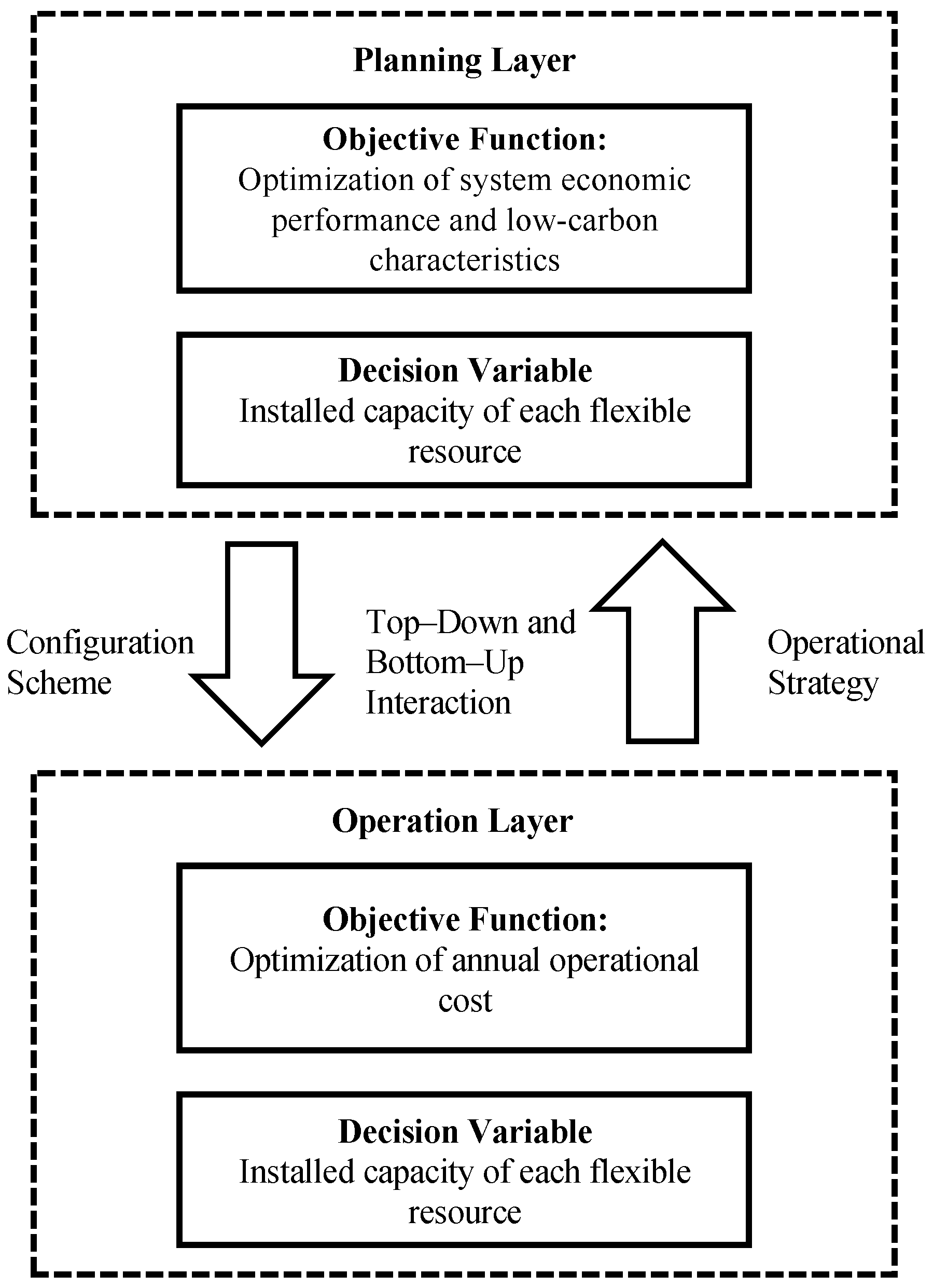
A two-level optimization framework is adopted to determine the optimal capacity allocation of various energy resources within the system. By establishing a coordinated operation–planning joint optimization model, the proposed two-level structure effectively balances both the economic performance and the operational flexibility of a system with a high penetration of renewable energy. The planning layer and the operation layer interact in a top–down and bottom–up manner, jointly determining the optimal configuration of flexible resources. The interaction mechanism is illustrated in Figure 2.

3.1. Operation Layer

3.1.1. Objective Function of the Operation Layer

In the operation layer, system operating cost, system revenue, and renewable energy consumption rate are adopted as performance evaluation indicators. The objective of the operation layer is to minimize the overall system cost by optimizing the output of flexible resources. The mathematical expression of the objective function is given as follows:

$$\min F_1=C_1+c_f{f}_{ex}-R$$

(19)

$$f_{ex}={\displaystyle \sum _{i=1}^M\frac{P_{\mathrm{total}}(t)-P_{\mathrm{use}}(t)}{P_{\mathrm{total}}(t)}}$$

(20)

where $F_1$ denotes the objective function of the operation layer; $C_1$ denotes the system operating cost; $R$ denotes the system revenue; $f_{ex}$ denotes the renewable-energy consumption rate; $P_{\mathrm{total}}(t)$ denotes the total power output of renewable energy sources (kW); and $P_{\mathrm{use}}(t)$ denotes the renewable energy power actually consumed by the users.

The operating cost of the system is given as:

$$\begin{array}{l}{C}_1={\mathrm{c}}_1{P}_{wt}+{\mathrm{c}}_2{P}_{pv}+{\mathrm{c}}_3{P}_{tide}+{\mathrm{c}}_4{P}_{wave}+{\mathrm{c}}_5{P}_{ess}+{\mathrm{c}}_6{P}_{ev}\\ +{\mathrm{c}}_7{P}_w+{\mathrm{c}}_8{P}_{h2}+{\mathrm{c}}_9{P}_{grid\_buy}{+\mathrm{c}}_9{P}_{ev}+{\mathrm{c}}_{10}{P}_w+{\mathrm{c}}_{11}{P}_{h2}\end{array}$$

(21)

where $P_{\mathrm{wt}}$ denotes the wind power output (kW); $P_{\mathrm{pv}}$ denotes the photovoltaic power output (kW); $P_{\mathrm{tide}}$ denotes the tidal current power output (kW); $P_{\mathrm{wave}}$ denotes the wave energy power output (kW); $P_{\mathrm{ess}}$ denotes the battery discharge power (kW); $P_{\mathrm{ev}}$ denotes the electric vehicle power; $P_{\mathrm{h}2}$ denotes the electrolyzer power (kW); $P_{\mathrm{w}}$ denotes the seawater desalination power; $P_{\mathrm{grid}\_\mathrm{buy}}$ denotes the purchased grid power (kW); $P_{\mathrm{grid}\_\mathrm{sell}}$ denotes the sold grid power (kW); and ${\mathrm{c}}_1$~${\mathrm{c}}_{11}$ denote the cost coefficients (CNY/kW) of different power equipment.

The revenue of the system is given as:

$$R={\mathrm{r}}_1{P}_{ev}+{\mathrm{r}}_2{P}_w+{\mathrm{r}}_3{P}_{h2}+{\mathrm{r}}_4{P}_{grid\_sell}$$

(22)

where ${\mathrm{r}}_1$~${\mathrm{r}}_4$ denote the revenue coefficients of power stations (CNY/kW).

3.1.2. Operational Constraints of the Operation Layer

The maximum–minimum power constraints of each unit are given as:

$$\left\{\begin{array}{c}{P}_{wt,\min }<P_{wt}<P_{wt,\max }\\ P_{pv,\min }<P_{pv}<P_{pv,\max }\\ P_{tide,\min }<P_{tide}<P_{tide,\max }\\ P_{wave,\min }<P_{wave}<P_{wave,\max }\\ P_{ev,\min }<P_{ev}<P_{ev,\max }\\ P_{w,\min }<P_w<P_{w,\max }\\ P_{h2,\min }<P_{h2}<P_{h2,\max }\end{array}\right.$$

(23)

The ramping constraints are given as:

$$0<d{P}_w<d{P}_{w,\max }$$

(24)

The maximum–minimum constraints of hydrogen production and freshwater output are given as:

$$Q_{P_w,\min }<Q_{P_w}<Q_{P_w,\max }$$

(25)

$$Q_{P_{h2,\min }}<Q_{P_{h2}}<Q_{P_{h2,\max }}$$

(26)

Energy Storage Constraints:

(1)

Dynamic State Balance

The state of charge (SOC) at time $t$ is updated recursively, where the SOC in the current time period equals the remaining energy of the previous time period plus the charging increment and minus the discharging consumption, and can be expressed as:

$$E_{\mathrm{ba}}(t+1)=E_{\mathrm{ba}}(t)+\left(P_t^{ba,c}\cdot {\eta }_{\mathrm{ba},c}-{\displaystyle \frac{P_t^{ba,d}}{{\eta }_{\mathrm{ba},\mathrm{d}}}}\right)\cdot \mathsf{\Delta }t,\forall t\in T.$$

(27)

$$0⩽P_t^{ba,c}⩽P_{\max }^{ba,c}$$

(28)

$$0⩽P_t^{ba,d}⩽P_{\max }^{ba,d}$$

(29)

(2)

SOC Boundary

The state of charge (SOC) of the energy storage system must remain within the safe operating range:

$$S_{\mathrm{OC}}(t)=E_{\mathrm{ba}}(t)/E_{\mathrm{ba},0}$$

(30)

$$S_{\mathrm{OC},\min }⩽S_{\mathrm{OC}}(t)⩽S_{\mathrm{OC},\max }$$

(31)

(3)

Charging–Discharging Mutual-Exclusion Constraint

The energy storage system cannot charge and discharge simultaneously at any time:

$$P_t^{ba,d}\cdot P_t^{ba,c}=0$$

(32)

3.2. Planning Layer

3.2.1. Objective Function of the Planning Layer

In the planning layer, system investment indicators are incorporated into the evaluation framework. The objective of the planning layer is to minimize the annual total cost of the system by comprehensively planning the capacities of flexible resources. The objective function is expressed as follows:

$$\min F_2=F_1+C_2$$

(33)

where $F_2$ denotes the objective function of the planning layer, and $C_2$ denotes the investment cost annualized by the interest rate.

The annualized investment cost of the system is given as:

$$C_2={\displaystyle \frac{r{(1+r)}^n}{{(1+r)}^n-1}}{\displaystyle \sum _{i=1}^{N_0}{c}_{\mathrm{i}}}{P}_i$$

(34)

3.2.2. Constraints

The maximum–minimum constraints on the number of units are given as:

$$\left\{\begin{array}{c}{N}_{WT,\min }<N_{WT}<N_{WT,\max }\\ N_{PV,\min }<N_{PV}<N_{PV,\max }\\ N_{WAVE,\min }<N_{WAVE}<N_{WAVE,\max }\\ N_{TI,\min }<N_{TI}<N_{TI,\max }\\ N_{ESS,\min }<N_{ESS}<N_{ESS,\max }\end{array}\right.$$

(35)

where $N_{WT,\min }$, $N_{PV,\min }$, $N_{WAVE,\min }$, $N_{TI,\min }$, and $N_{ESS,\min }$ denote the required minimum number of wind turbine units, photovoltaic units, wave energy units, tidal current energy units, and battery storage units in the system, respectively; $N_{WT,\max }$, $N_{PV,\max }$, $N_{WAVE,\max }$, $N_{TI,\max }$, and $N_{ESS,\max }$ denote the allowed maximum number of wind turbine units, photovoltaic units, wave energy units, tidal current energy units, and battery storage units in the system, respectively.

4. Optimal Scheduling Model

Considering that the prediction errors of wind power, photovoltaic output, and offshore renewable energy generation decrease as the time scale becomes shorter, this paper proposes a multi-time-scale rolling optimization scheduling strategy that incorporates both day-ahead and intra-day scheduling.

In the day-ahead scheduling stage, the objective is to maximize the economic benefits of system operation. Based on the short-term forecasts of wind power, photovoltaic output, tidal current power, wave energy output, and system load, a scheduling interval of 1 h is adopted. Under the premise of meeting the load demand for the upcoming day, and by considering the output characteristics of each distributed energy source, as well as the charging and discharging power limits of the energy storage devices, a system-level economic optimal scheduling model is established. The solution of this model provides the dispatch plan for each distributed generation unit at each time interval for the following day, enabling coordinated economic operation through reasonable scheduling of distributed energy units, energy storage devices, and tie-line power exchanges.

In the intra-day scheduling stage, rolling optimization is performed with a scheduling interval of 1 h and a rolling horizon of 4 h. Since the day-ahead dispatch plan may deviate from real-time operational conditions due to uncertainties in wind, photovoltaic, tidal current, and wave outputs, as well as load variations, it cannot be directly applied to practical system operation. Therefore, an intra-day scheduling model is constructed based on ultra-short-term forecasts of uncontrollable renewable resources and load demand. Subject to the operational constraints of each device and relevant energy balance constraints, the objective is to minimize power fluctuations and operating cost. The model continuously updates the scheduled outputs of distributed energy units and energy storage devices through rolling corrections, and real-time power sampling of distributed sources is performed to ensure feedback-based adjustment and compensation.

4.1. Day-Ahead Scheduling

4.1.1. Objective Function

The day-ahead scheduling plan is obtained by minimizing the system operating cost, maximizing system revenue, and improving the renewable-energy consumption rate. The objective function is consistent with the operation-layer objective defined in (19)–(22).

4.1.2. Constraints

The constraints include the maximum–minimum power limits of each unit (23); ramping constraints (24); maximum–minimum limits of hydrogen production and freshwater output (25) and (26); and the energy storage constraints (27)–(32).

4.2. Intra-Day Rolling Scheduling

The objective of the intra-day rolling scheduling model is to minimize the cost while mitigating the intra-day fluctuations of renewable energy. The objective function is given as follows:

$$\min F_3=C_{rt1}+C_{rt2}+C_{rt3}$$

(36)

where $F_3$ denotes the objective function of the intra-day scheduling model; $C_{rt1}$ denotes the system regulation cost; $C_{rt2}$ denotes the system operating cost; and $C_{rt3}$ denotes the renewable-energy curtailment cost.

The regulation cost of the system is given as:

$$\begin{array}{l}{C}_{rt1}={\eta }_1{(P_{ess\_rt}-P_{ess})}^2+{\eta }_2{(P_{ev\_rt}-P_{ev})}^2+{\eta }_3{(P_{w\_rt}-P_w)}^2\\ +{\eta }_4{(P_{h2\_rt}-P_{h2})}^2+{\eta }_5{(P_{grid\_rt}-P_{grid})}^2\end{array}$$

(37)

where ${\eta }_1$~${\eta }_5$ denote the intra-day power adjustment cost coefficients (CNY/kW).

$$\begin{array}{l}{C}_{rt2}={\mathrm{c}}_1{P}_{wt\_rt}+{\mathrm{c}}_2{P}_{pv\_rt}+{\mathrm{c}}_3{P}_{tide\_rt}+{\mathrm{c}}_4{P}_{wave\_rt}+{\mathrm{c}}_5{P}_{ess\_rt}+{\mathrm{c}}_6{P}_{ev\_rt}+{\mathrm{c}}_7{P}_{w\_rt}+{\mathrm{c}}_8{P}_{h2\_rt}\\ +{\mathrm{c}}_9{P}_{grid\_buy\_rt}+{\mathrm{c}}_9{P}_{ev\_rt}+{\mathrm{c}}_{10}{P}_{w\_rt}+{\mathrm{c}}_{11}{P}_{h2\_rt}-{\mathrm{r}}_1{P}_{ev\_rt}-{\mathrm{r}}_2{P}_{w\_rt}-{\mathrm{r}}_3{P}_{h2\_rt}+{\mathrm{r}}_4{P}_{grid\_sell\_rt}\end{array}$$

(38)

The renewable-energy curtailment cost of the system is given as:

$$\begin{array}{l}{C}_{rt3}=f_1(P_{wt\_rt}-P_{wt\_n})+f_2(P_{pv\_rt}-P_{pv\_n})\\ +f_3(P_{ti\_rt}-P_{ti\_n})+f_4(P_{wave\_rt}-P_{wave\_n})\end{array}$$

(39)

where $f_1$~$f_4$ denote the intra-day renewable-energy curtailment cost coefficients (CNY/kW).

4.3. Network Constraints of Power System

Each transmission line (including both AC and DC lines) has an upper limit on the maximum allowable power that can pass through it. It can be expressed as:

$$\left|P_{\mathrm{ij}}\right|⩽P_{\mathrm{ij}}^{\max }$$

(40)

where $P_{\mathrm{ij}},P_{\mathrm{ij}}^{\max }$ are the transmission line power and the upper limit power of transmission line power.

The calculation formula for distribution network losses is as follows:

$$P^{LOSS}={\displaystyle \sum _l{r}_l}{(F_l)}^2\approx {\displaystyle \sum _l{r}_l}{(P_l^f)}^2$$

(41)

$$Q^{LOSS}={\displaystyle \sum _l{x}_l}{(F_l)}^2\approx {\displaystyle \sum _l{x}_l}{(Q_l^f)}^2$$

(42)

where $F_l$ represents the current of line l. The branch network losses can be expressed as the product of loss factors and the net injected power at nodes, plus a deviation term.

Moreover, this study emphasized that the results are preliminary and intended to identify high-level trends rather than provide precise operational guidelines.

5. Case Study Analysis

5.1. Basic Data and Parameters

In terms of capacity configuration, the scale of the EV charging demand, freshwater demand, and hydrogen production demand at the project site is first used to determine the capacities of the EV charging system, seawater desalination system, and electrolysis system. The EV capacity is set to 200 kW, the seawater desalination capacity is set to 500 kW, and the hydrogen production capacity is set to 400 kW. The remaining parameters are listed in

Table 1. Rated Capacity of Single Units.

Unit Type	Capacity per Unit (kW)
Wind turbine	1500
Solar panel	0.6
Wave energy device	50
Tidal current device	70
Battery module	300

,

Table 2. Investment Cost of Equipment.

Unit Type	Investment Cost (CNY/kW)	Lifetime (Years)
Wind turbine	14,000	30
Solar power equipment	5800	20
Wave energy device	20,000	25
Tidal current device	16,000	25
Battery module	1500	10

and

Table 3. Operation and Maintenance Levelized Cost of Electricity (LCOE).

Unit Type	LCOE (CNY/kW)
Wind turbine	0.15
Solar power equipment	0.1
Wave energy device	0.3
Tidal current device	0.25
Battery module	0.13
Electric vehicle system	−0.5
Hydrogen production unit	−0.7
Seawater desalination	−0.8

.

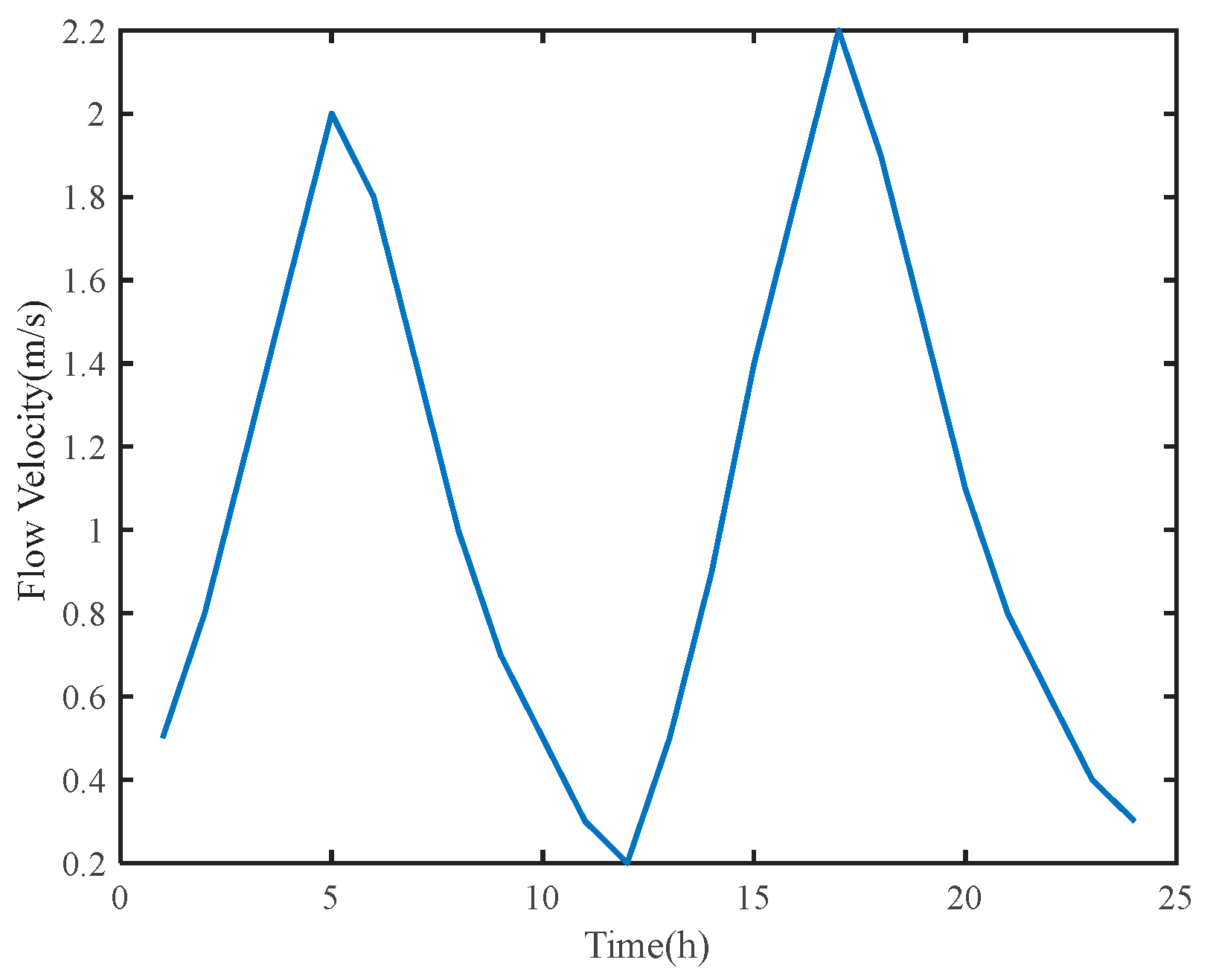
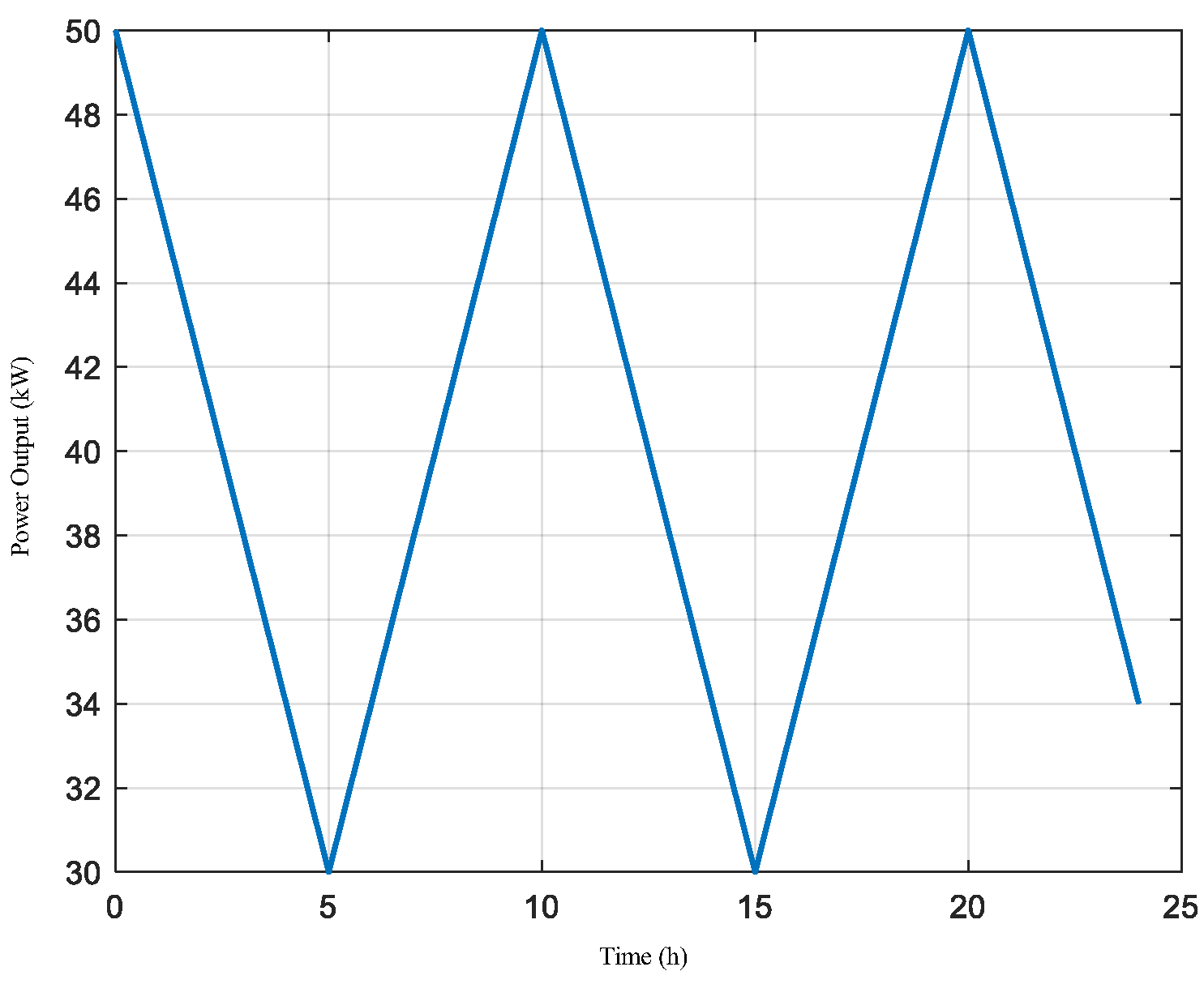
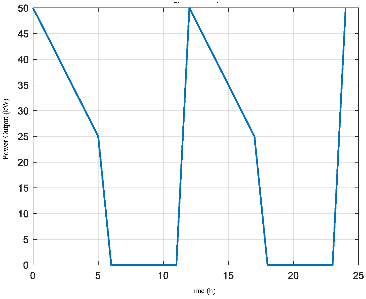
The tidal current velocity profile is given in Figure 3. The wave energy output differs under large-wave and small-wave operating conditions; the specific outputs are shown in Figure 4 and Figure 5. In this case study, the wave energy device is assumed to operate under the large-wave condition throughout [31].

5.2. Continuous Operating Conditions and Intermittent Operating Conditions

In the system dispatch optimization stage, the installed capacities are set as follows: 4500 kW of wind turbines, 2100 kW of photovoltaic units, 1050 kW of tidal current units, 1000 kW of wave energy units, and 1200 kW of battery storage. The adjustment cost parameters for load-side resources and battery storage are listed in

Table 4. Cost Coefficients for Intra-day Power Adjustment.

Type	Adjustment Cost/kW (Yuan)
Tie-line power	0.02
Electrolytic hydrogen unit	0.1
Seawater desalination unit	0.1
Electric vehicle unit	0.05
Battery storage	0.2

, while the curtailment cost coefficients for renewable energy units are provided in

Table 5. Curtailment Cost Coefficients for Intra-day Renewable Power.

Type	Curtailment Cost/kW (Yuan)
Wind turbine	0.3
Photovoltaic unit	0.3
Wave energy unit	0.2
Tidal current unit	0.2

.

5.3. Analysis of Capacity Configuration Optimization Results

This paper employs an improved Particle Swarm Optimization (PSO) algorithm, which aims to overcome the drawbacks of basic PSO, such as its tendency to get trapped in local optima and its slow convergence speed. The algorithm enhances its performance by introducing various strategies, specifically by gradually decreasing the inertia weight from its maximum to its minimum value. This approach enables the algorithm to possess strong global search capabilities in the early stages and robust local convergence capabilities in the later stages. While this method is simple and effective, it may not be adaptable to the characteristics of all problems.

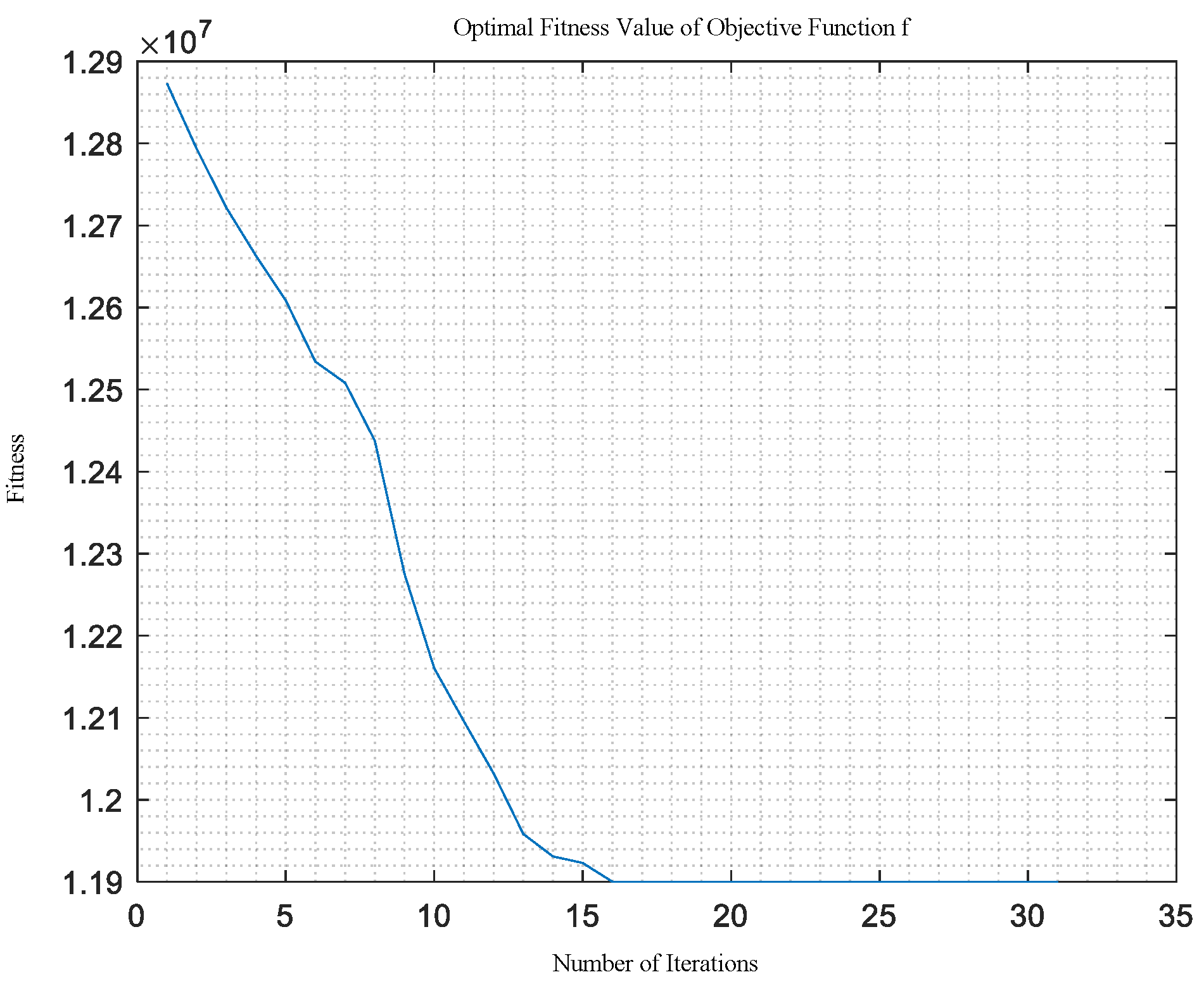
By employing an improved particle swarm optimization (PSO) algorithm, the convergence behavior is illustrated in Figure 6. The final capacity configuration is summarized in

Table 6. Capacity Allocation Results.

Resource Type	Number of Wind Turbines	Number of PV Panels	Number of Tidal Units	Number of Wave Units	Number of Battery Units	Net Cost (Yuan)	Curtailment Rate
Configuration	3	350	15	20	8	1.19 × 107	0.7%

, yielding a configuration of 4500 kW wind power, 2100 kW photovoltaic capacity, 1050 kW tidal current generation, 1000 kW wave energy generation, and 2400 kW battery storage. Under this configuration, the minimum net cost is 1.19 × 10⁷, and the curtailment rate is reduced to only 0.7%.

A comprehensive sensitivity analysis is shown in

Table 7. Sensitivity analysis.

Resource Type	Number of Wind Turbines	Number of PV Panels	Number of Tidal Units	Number of Wave Units	Number of Battery Units	Net Cost (Yuan)	Curtailment Rate
Scenario 1	4	350	15	20	8	1.21 × 107	1%
Scenario 2	3	385	15	20	8	1.25 × 107	0.8%
Scenario 3	3	350	17	20	8	1.72 × 107	1.3%
Scenario 4	3	350	15	22	8	1.69 × 107	1.1%
Scenario 5	3	350	15	20	9	1.45 × 107	0%

. We set up five scenarios to analyze the sensitivity of the optimization results corresponding to Table 6, where each optimized variable is increased by 10%, and then analyze the outcomes of net cost and curtailment. The results demonstrate that the proposed configuration remains relatively stable and robust under a reasonable range of parameter changes, which significantly strengthens the conclusions of our study.

5.4. System Optimization and Scheduling Results Analysis

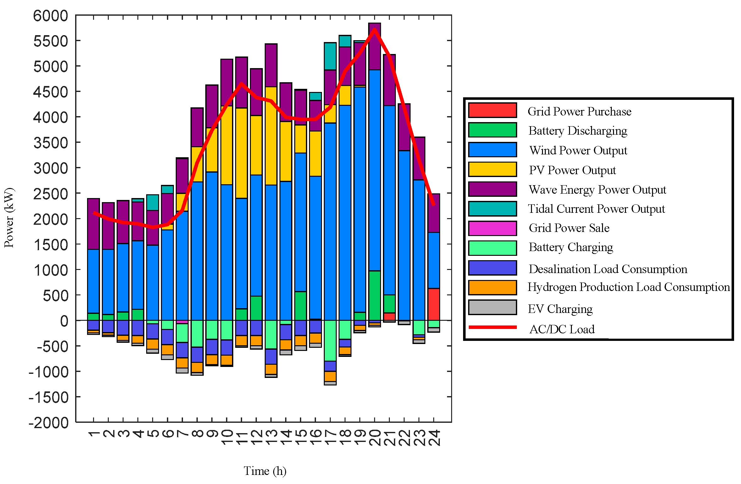
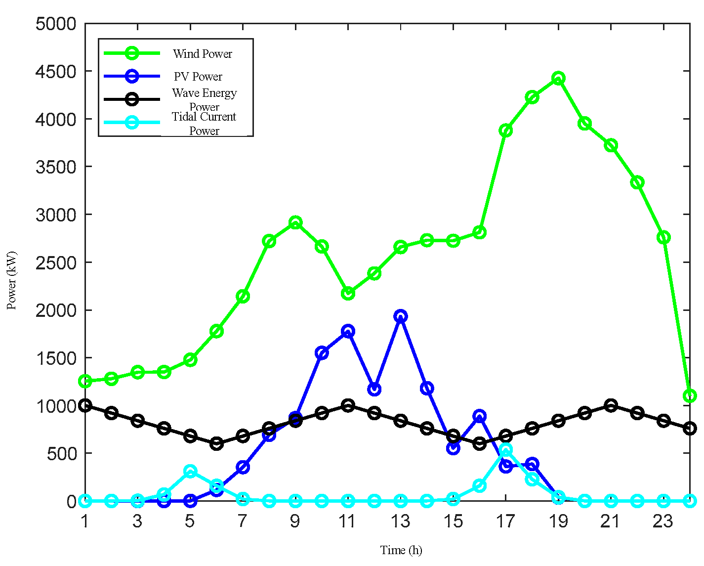
The day-ahead scheduling results are illustrated in Figure 7, Figure 8, Figure 9 and Figure 10. Under the optimal capacity configuration, renewable energy generation is abundant. Figure 11 presents the output profiles of each renewable energy source. Wind power exhibits the largest available capacity. Photovoltaic generation starts to produce electricity from approximately 07:00 and continues until 18:00. Tidal energy production is determined by the gravitational interactions among the Earth, the Moon, and the Sun. The tidal phenomenon produces two high tides and two low tides per day, with a cycle of approximately 12 h 24 min (semi-diurnal tide), resulting in a periodic pattern in the tidal current output within a single day. Wave energy output fluctuates between 600 kW and 420 kW under large-wave operating conditions.

We have included data and results from at least 7-day scenarios in the revised manuscript. These extended scenarios cover different seasons, allowing us to better account for the seasonal fluctuations in renewable energy generation. We have analyzed the solar power output over a 7-day period in both summer and winter, considering factors such as varying daylight hours and cloud cover. Similarly, for wind power, we have examined data from multiple 7-day intervals across different seasons to capture the changes in wind speed and direction.

As shown in Figure 7 and Figure 8, the system satisfies the power balance constraints. Due to the high availability of renewable energy, the seawater desalination unit, electric vehicle charging stations, and electrolyzer fully absorb the surplus renewable electricity, achieving multi-channel utilization and economic efficiency.

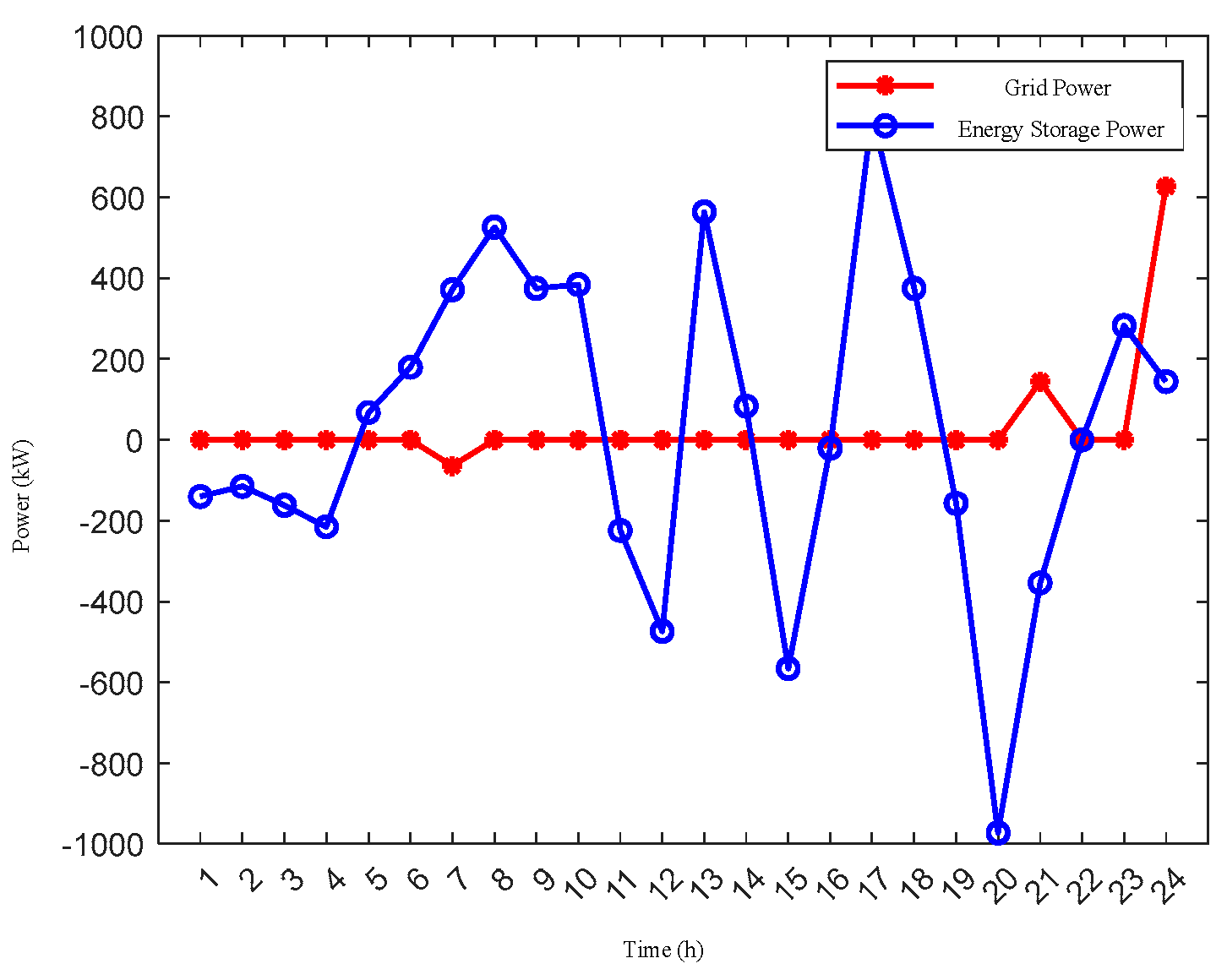
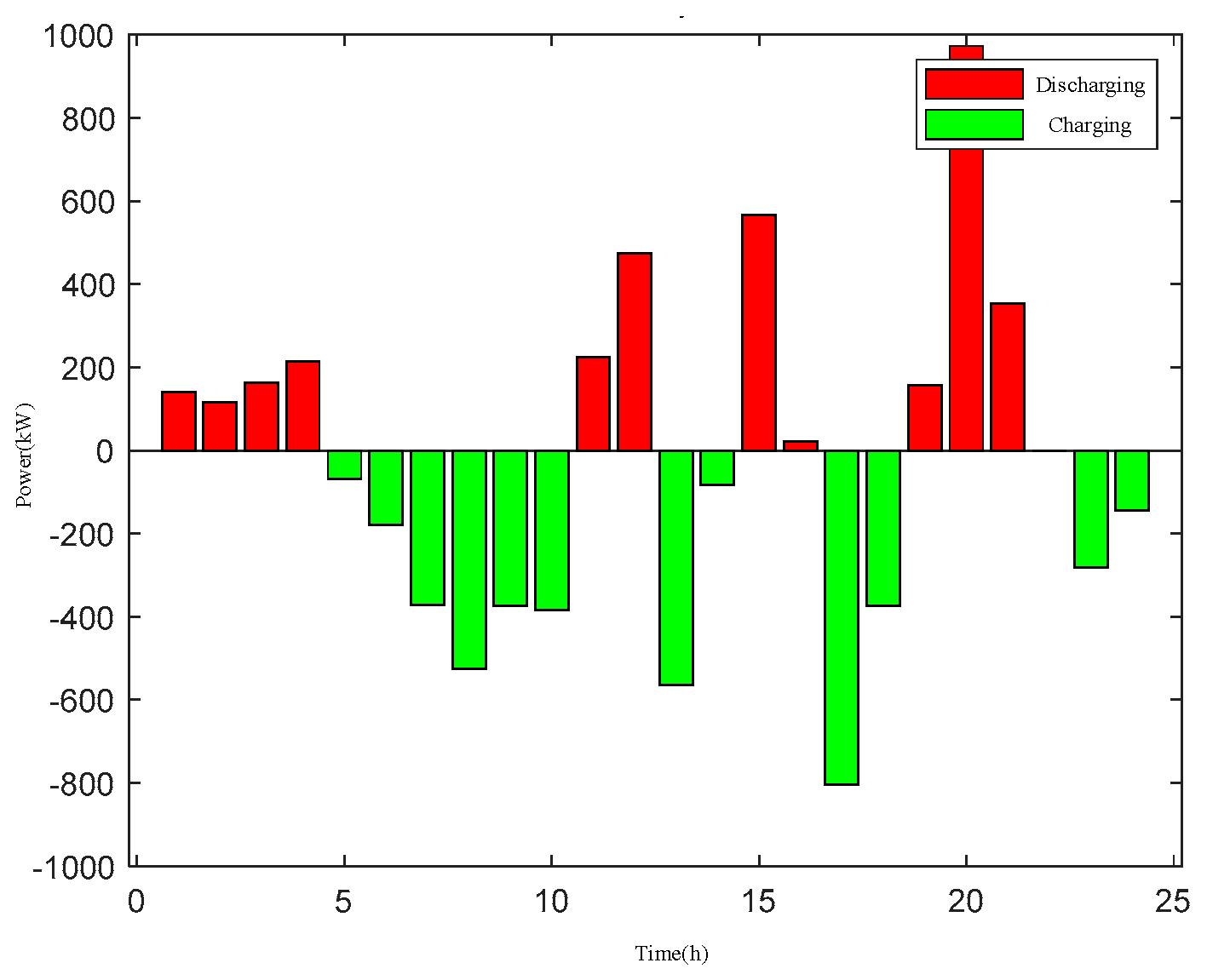
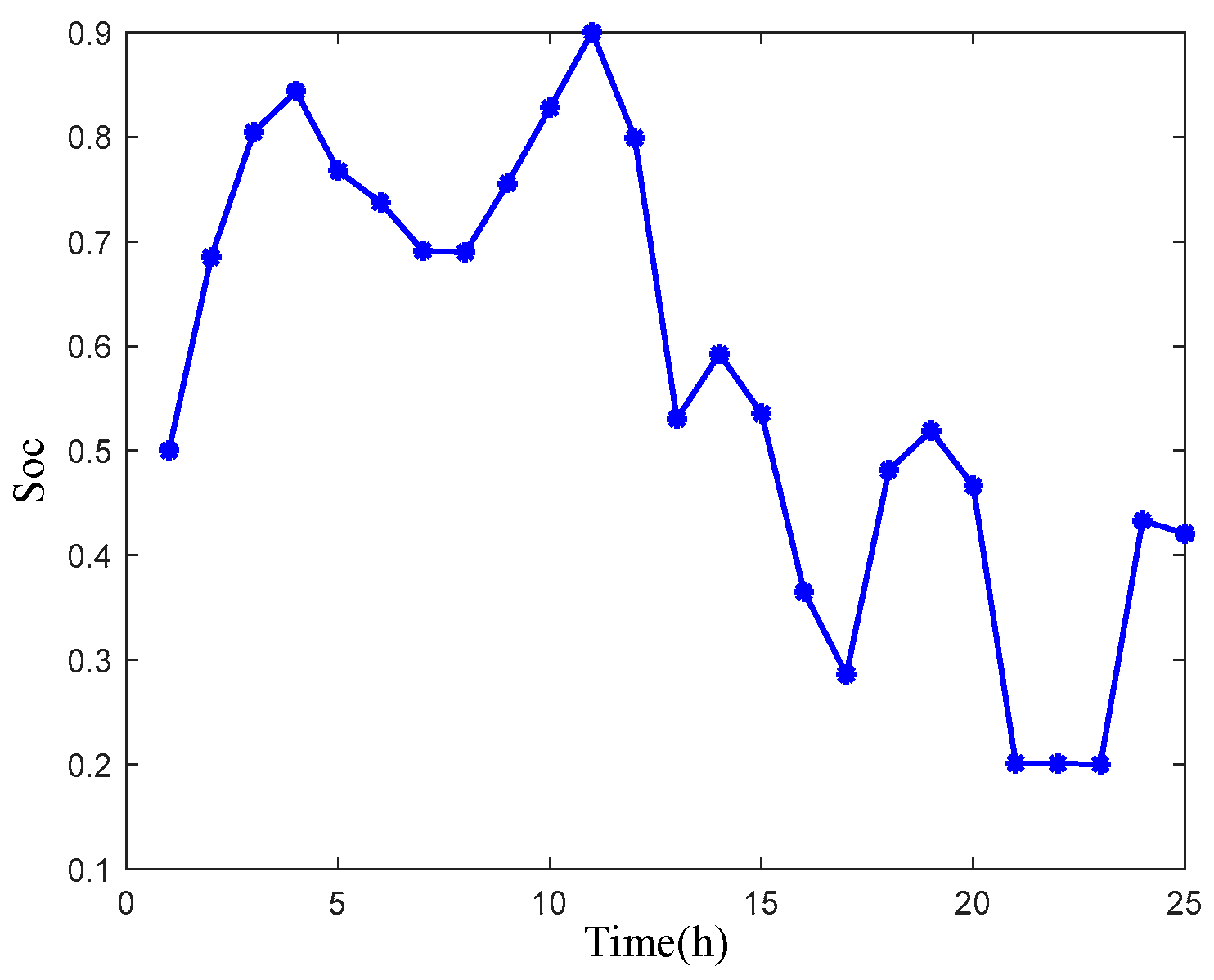
Energy storage output is given in Figure 10 and Figure 11. The storage system charges during low-price periods and discharges during high-price periods, improving overall system revenue by leveraging the intrinsic arbitrage characteristics of energy storage. Meanwhile, the state of charge (SOC) at the end of each day is maintained within 5% of the initial state, ensuring safe and stable operation.

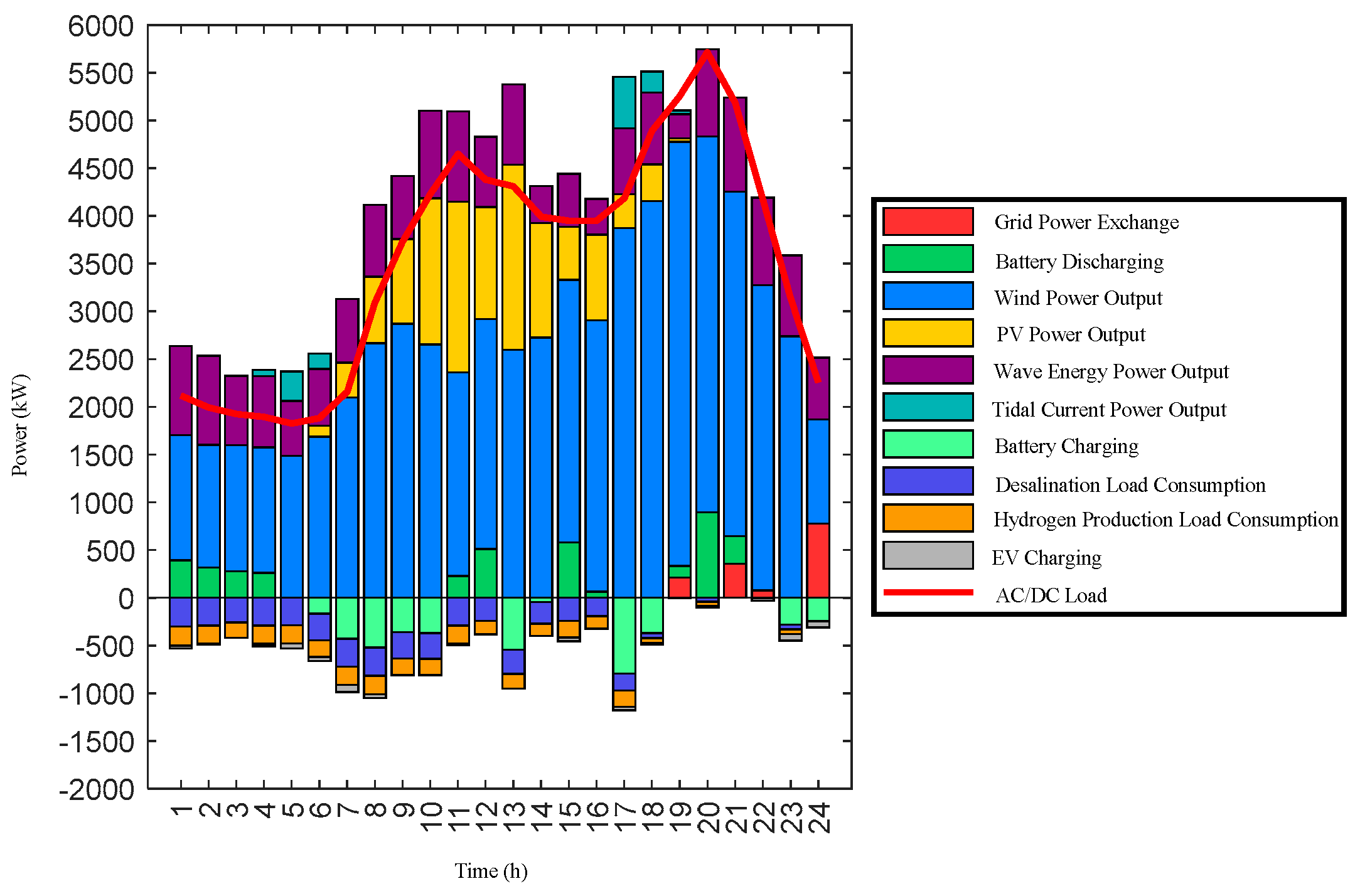
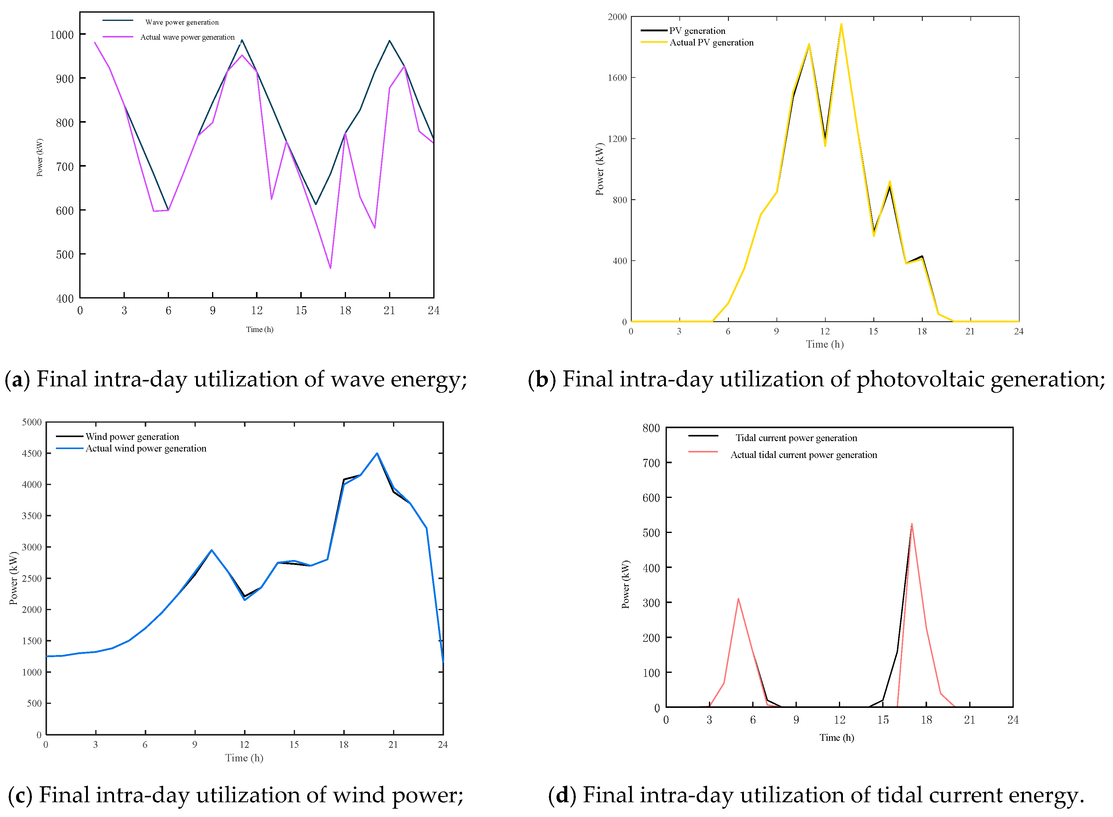
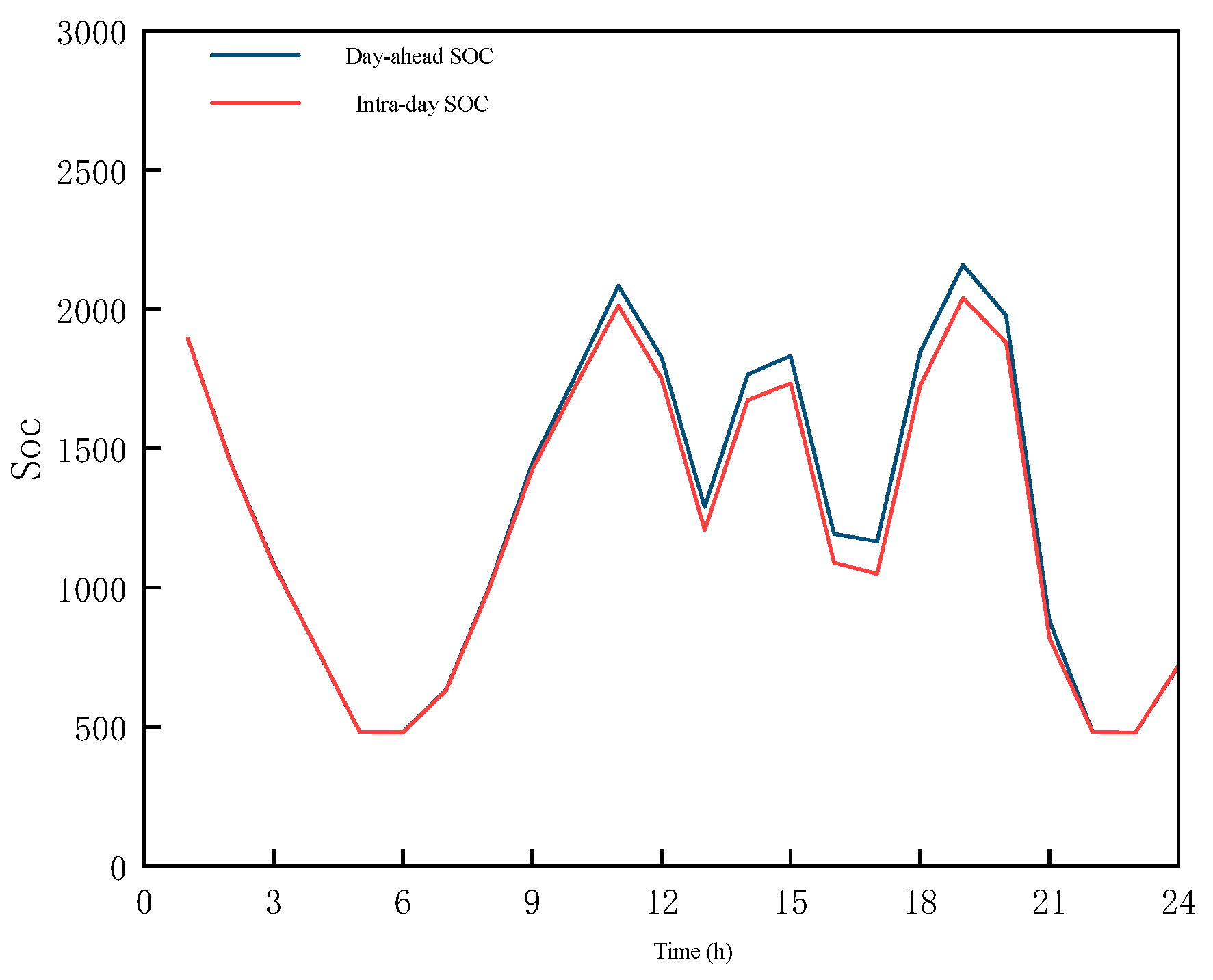
As illustrated in Figure 12, the system maintains power balance by adjusting energy storage units, tie-line power flows, and load-side flexible resources, thereby accommodating the real-time fluctuations of renewable energy. Figure 13 shows that renewable energy utilization is satisfactory, with only minor curtailment occurring in wave and tidal generation. The proposed rolling optimization strategy effectively mitigates wind and solar curtailment. The scheduling results of the energy storage system are presented in Figure 14, where the state of charge also satisfies the operational constraints, and the deviation from the day-ahead SOC remains within 10%.

The intra-day rolling scheduling adopts a 1 h time window and continuously updates the scheduling plan for the subsequent 4 h. Compared with conventional single-stage day-ahead scheduling, this approach effectively reduces the forecasting errors of renewable generation during the execution period. Through the rolling correction mechanism, the wind–solar output trajectories are continuously recalibrated, which significantly improves the reliability and applicability of the forecasted data.

The rapid regulation capability of electrochemical energy storage provides sufficient buffer capacity for instantaneous power fluctuations, making it particularly suited for mitigating typical variability scenarios such as midday photovoltaic power drops or nighttime wind-power surges. On the demand side, resources such as electric vehicles and seawater desalination facilities absorb excess renewable generation during high-output periods by shifting their loads, and reduce non-essential demand during low-output periods, thereby enhancing the system’s flexibility in responding to renewable energy fluctuations.

Overall, the coordinated optimization across day-ahead and intra-day timescales, combined with the flexible regulation of multiple resources, substantially improves the system’s ability to accommodate fluctuations in renewable energy generation.

6. Conclusions

This study focuses on an offshore multi-energy coupling system and conducts systematic research on capacity optimization and rolling scheduling. A two-stage optimization framework featuring coordinated operation–planning on assumptions data is proposed. The main conclusions are as follows:

(1)

A comprehensive multi-energy coupling system model is constructed, integrating wind power, photovoltaic generation, tidal current energy, wave energy, energy storage, hydrogen production by electrolysis, and seawater desalination loads. The model characterizes the complementary relationships among energy units and clarifies the energy flow pathways, thereby providing a solid foundation for optimal operation of offshore integrated energy systems.

(2)

A bi-level capacity configuration method based on coordinated operation–planning optimization is proposed. At the planning level, the annualized total system cost is minimized to achieve a rational allocation of energy and storage units. At the operation level, economic performance and system flexibility are jointly optimized to determine the optimal configuration of flexible resources.

(3)

A multi-timescale rolling dispatch model is designed, integrating day-ahead and intra-day collaborative optimization mechanisms. This enables dynamic adjustments and real-time correction of system operations, significantly enhancing the system’s capability to accommodate renewable energy fluctuations and improve energy utilization efficiency. Simulation results indicate that the proposed method reduces the curtailment rate to 0.7%, markedly improving system economy and stability.

(4)

The research validates the feasibility and effectiveness of coordinated operation–planning and rolling scheduling strategies, offering a new technical roadmap and theoretical basis for capacity configuration and operational optimization in offshore multi-energy systems. Future research may further incorporate uncertainty modeling and market-responsive mechanisms, and explore coordinated strategies for energy storage control and multi-agent decision-making, promoting the intelligent and economic development of offshore integrated energy systems. Our findings are intended to provide insights for future research and development rather than immediate operational guidelines.

References

- Zaidi, S.; Abbas, M.K.; Saleem, S.; Khan, B.M.; Haider, S. Renewable Tidal Power Generation Significance & Challenges. In Proceedings of the 2021 International Bhurban Conference on Applied Sciences and Technologies (IBCAST), Islamabad, Pakistan, 12–16 January 2021; pp. 1–6. [Google Scholar] [CrossRef]
- Dhabliya, D.; Varshney, N.; Sasikumar, M.; Vijayaraghavan, P.; Vimala, M.; Sapaev, J.B.; Almusawi, M.; Ushasree, D. Harnessing Tidal Energy: Design and Performance Evaluation of Marine Energy Conversion Systems. In Proceedings of the 2023 International Conference for Technological Engineering and its Applications in Sustainable Development (ICTEASD), AL-Najaf, Iraq, 20–23 August 2023; pp. 190–195. [Google Scholar] [CrossRef]
- Singh, D.; Verma, P.; Nema, R. Harnessing the Power of Nature: A Short Review of Renewable Energy Resources. In Proceedings of the 2024 IEEE International Students’ Conference on Electrical, Electronics and Computer Science (SCEECS), Bhopal, India, 24–25 February 2024; pp. 1–7. [Google Scholar] [CrossRef]
- Ma, X.; Wang, D.; Zhao, Z.; Lu, C.; Wang, C.; Liu, B.; Zhang, X.; Zhu, S. Preliminary Exploration on the Integrated Development of Offshore Wind Power Industry. In Proceedings of the 2025 International Conference on Smart Grid and Sustainable Energy (SGSE), Guangzhou, China, 12–14 December 2025; pp. 1–6. [Google Scholar] [CrossRef]
- Gong, Y.; Yang, Z.B.; Shan, X.B.; Sun, Y.B.; Xie, T.; Zi, Y.L. Capturing Flow Energy from Ocean and Wind. Energies 2019, 12, 2184. [Google Scholar] [CrossRef]
- Marino, E.; Gkantou, M.; Malekjafarian, A.; Bali, S.; Baniotopoulos, C.; van Beeck, J.; Borg, R.P.; Bruschi, N.; Cardiff, P.; Chatzi, E.; et al. Offshore renewable energies: A review towards Floating Modular Energy Islands-Monitoring, Loads, Modelling and Control. Ocean Eng. 2024, 313, 20. [Google Scholar] [CrossRef]
- Kamali-Sarvestani, R.; Nademi, H. Harnessing the Power of Ocean Waves to Make Electric Energy. In Proceedings of the 9th Annual IEEE Conference on Technologies for Sustainability (IEEE SusTech), ELECTR NETWORK, Riverside, CA, USA, 21–23 April 2022; pp. 173–176. [Google Scholar]
- Wiegner, J.F.; Andreasson, L.M.; Kusters, J.E.H.; Nienhuis, R.M. Interdisciplinary perspectives on offshore energy system integration in the North Sea: A systematic literature review. Renew. Sustain. Energy Rev. 2024, 189, 23. [Google Scholar] [CrossRef]
- Santhakumar, S.; Meerman, H.; Faaij, A.; Gordon, R.M.; Gusatu, L.F. The future role of offshore renewable energy technologies in the North Sea energy system. Energy Convers. Manag. 2024, 315, 15. [Google Scholar] [CrossRef]
- Kazemi-Robati, E.; Silva, B.; Bessa, R.J. Stochastic optimization framework for hybridization of existing offshore wind farms with wave energy and floating photovoltaic systems. J. Clean. Prod. 2024, 454, 18. [Google Scholar] [CrossRef]
- Gao, Q.; Bechlenberg, A.; Jayawardhana, B.; Ertugrul, N.; Vakis, A.I.; Ding, B.Y. Techno-economic assessment of offshore wind and hybrid wind-wave farms with energy storage systems. Renew. Sustain. Energy Rev. 2024, 192, 12. [Google Scholar] [CrossRef]
- Dallavalle, E.; Zanuttigh, B.; Contestabile, P.; Giuggioli, A.; Speranza, D. Improved methodology for the optimal mixing of renewable energy sources and application to a multi-use offshore platform. Renew. Energy 2023, 210, 575–590. [Google Scholar] [CrossRef]
- Elginoz, N.; Bas, B. Life Cycle Assessment of a multi-use offshore platform: Combining wind and wave energy production. Ocean Eng. 2017, 145, 430–443. [Google Scholar] [CrossRef]
- Chen, P.H.; Wu, D.W. A review of hybrid wave-tidal energy conversion technology. Ocean Eng. 2024, 303, 14. [Google Scholar] [CrossRef]
- Zhang, N.B.; Li, C.X.; Li, Z.; Liu, P. Strategies for sustainable development of offshore wind power in regions with limited resources. Energy 2024, 311, 17. [Google Scholar] [CrossRef]
- Gangil, G.; Goyal, S.K.; Saraswat, A. A multi-objective techno-economic operation of distribution network considering reactive power support from renewable energy and battery storage system. J. Energy Storage 2024, 102, 18. [Google Scholar] [CrossRef]
- Megantoro, P.; Abd Halim, S.; Kamari, N.A.M.; Awalin, L.J.; Mohamed, R.; Rosli, H.M. An enhanced multi-objective reactive power dispatch for hybrid Wind-Solar power system using Archimedes optimization algorithm. Int. J. Electr. Power Energy Syst. 2025, 168, 19. [Google Scholar] [CrossRef]
- Yin, Y.; Liu, T.Q.; Wu, L.; He, C.; Liu, Y.K. Day-ahead Risk-constrained Stochastic Scheduling of Multi-energy System. J. Mod. Power Syst. Clean Energy 2021, 9, 720–733. [Google Scholar] [CrossRef]
- Liu, S.W.; Yang, Z.B.; Du, Y.C.; Kong, F.X.; Ding, Y.R.; Wang, X.C. Day-Ahead Hierarchical Optimal Scheduling for Offshore Integrated Electricity-Gas-Heat Energy System Considering Load Forecasting. In Proceedings of the 45th Annual Conference of the IEEE Industrial Electronics Society (IECON), Lisbon, Portugal, 14–17 October 2019; IEEE: New York, NY, USA, 2019; pp. 2342–2347. [Google Scholar]
- Wang, J.; Zhao, Z.P.; Zhou, J.L.; Cheng, C.T.; Su, H.Y. Co-optimization for day-ahead scheduling and flexibility response mode of a hydro-wind-solar hybrid system considering forecast uncertainty of variable renewable energy. Energy 2024, 311, 22. [Google Scholar] [CrossRef]
- Liu, X.H.; Xie, S.H.; Tian, J.Q.; Wang, P. Two-Stage Scheduling Strategy for Integrated Energy Systems Considering Renewable Energy Consumption. IEEE Access 2022, 10, 83336–83349. [Google Scholar] [CrossRef]
- Ovstebo, M.L.; Naversen, C.O.; Helsetht, A.; Farahmand, H. Continuous-time scheduling of a hydrothermal system with integration of offshore wind power. In Proceedings of the 17th International Conference on the European Energy Market (EEM), Stockholm, Sweden, 16–18 September 2020; IEEE: New York, NY, USA, 2020. [Google Scholar]
- Zhang, Y.; Sun, H.; Tan, J.; Li, Z.; Hou, W.; Guo, Y. Capacity configuration optimization of multi-energy system integrating wind turbine/photovoltaic/hydrogen/battery. Energy 2022, 252, 124046. [Google Scholar] [CrossRef]
- Liu, H.; Xu, Y.; Yan, R.; Wang, Q. Capacity allocation optimization of power-hydrogen multi-energy microgrid including offshore wind power, underwater compressed air energy storage. J. Energy Storage 2025, 133, 117973. [Google Scholar] [CrossRef]
- Fu, J.; Zeng, G.; Ji, Y.; Zhou, A. Development of a Capacity Allocation Model for the Multi-Energy Hybrid Power System. J. Therm. Sci. 2025, 34, 936–952. [Google Scholar] [CrossRef]
- Shen, W.J.; Zeng, B.; Zeng, M. Multi-timescale rolling optimization dispatch method for integrated energy system with hybrid energy storage system. Energy 2023, 283, 16. [Google Scholar] [CrossRef]
- Huang, S.J.; Lu, H.; Chen, M.Z.; Zhao, W.J. Integrated energy system scheduling considering the correlation of uncertainties. Energy 2023, 283, 13. [Google Scholar] [CrossRef]
- Dong, F.X.; Wang, J.J.; Xu, H.W.; Zhang, X.T. A robust real-time energy scheduling strategy of integrated energy system based on multi-step interval prediction of uncertainties. Energy 2024, 300, 19. [Google Scholar] [CrossRef]
- Wang, Z.; Hou, H.; Zhao, B.; Zhang, L.; Shi, Y.; Xie, C. Risk-averse stochastic capacity planning and P2P trading collaborative optimization for multi-energy microgrids considering carbon emission limitations: An asymmetric Nash bargaining approach. Appl. Energy 2024, 357, 45–47. [Google Scholar] [CrossRef]
- Chang, L.; Li, Z.; Tian, X.; Su, J.; Chang, X.; Xue, Y.; Li, Z.; Jin, X.; Wang, P.; Sun, H. A two-stage distributionally robust low-carbon operation method for antarctic unmanned observation station integrating virtual energy storage and hydrogen waste heat recovery. Appl. Energy 2025, 400, 78–84. [Google Scholar] [CrossRef]
- Xiao, Y.; Ye, B.; Zhang, H.; Yuan, Y.; Zhou, B.; Jin, P.; Kang, J. Optimization of motion and power performance of a wind-wave hybrid system with built-in wave energy converters. Energy 2025, 339, 191–201. [Google Scholar] [CrossRef]
Figure 1.
Structure of the Multi-Energy Coupling DC Microgrid System.
Figure 2.
Capacity Configuration Process.
Figure 3.
Tidal Current Velocity.
Figure 4.
Wave Energy Output under continuous operation.
Figure 5.
Wave Energy Output under intermittent operation.
Figure 6.
Iteration Process.
Figure 7.
Day-ahead total resource output.
Figure 8.
Renewable energy generation output.
Figure 9.
Power exchange profile.
Figure 10.
Energy storage output.
Figure 11.
State of charge (SOC).
Figure 12.
Intra-day output of energy resources.
Figure 13.
Intra-day renewable energy utilization performance.
Figure 14.
State-of-charge scheduling results of the energy storage system.