Restoration of Distribution Network Power Flow Solutions Considering the Conservatism Impact of the Feasible Region from the Convex Inner Approximation Method

Abstract

Under the “Dual Carbon” strategy, high-penetration integration of distributed generators (DG) into distribution networks has triggered bidirectional power flow and reactive power-voltage violations. This phenomenon undermines the accuracy guarantee of conventional relaxation models (represented by second-order cone programming, SOCP), causing solutions to deviate from the AC power flow feasible region. Notably, ensuring solution feasibility becomes particularly crucial in engineering practice. To address this problem, this paper proposes a collaborative optimization framework integrating convex inner approximation (CIA) theory and a solution recovery algorithm. First, a system relaxation model is constructed using CIA, which strictly enforces ACPF constraints while preserving the computational efficiency of convex optimization. Second, aiming at the conservatism drawback introduced by the CIA method, an admissible region correction strategy based on Stochastic Gradient Descent is designed to narrow the dual gap of the solution. Furthermore, a multi-objective optimization framework is established, incorporating voltage security, operational economy, and renewable energy accommodation rate. Finally, simulations on the IEEE 33/69/118-bus systems demonstrate that the proposed method outperforms the traditional SOCP approach in the 24 h sequential optimization, reducing voltage deviation by 22.6%, power loss by 24.7%, and solution time by 45.4%. Compared with the CIA method, it improves the DG utilization rate by 30.5%. The proposed method exhibits superior generality compared to conventional approaches. Within the upper limit range of network penetration (approximately 60%), it addresses the issue of conservative power output of DG, thereby effectively promoting the utilization of renewable energy.

1. Introduction

By the end of 2024, the total installed capacity of wind and solar power in China reached 1.41 billion kW, accounting for approximately 42% of the total installed capacity. For the first time, the scale of renewable energy generation capacity has exceeded that of coal-fired power [1]. The structure and characteristics of distribution networks have undergone significant transformations due to the integration of various types of distributed energy resources (DER), leading to a gradual transition toward Active Distribution Networks (ADN).

Although system flexibility and economic efficiency are enhanced by ADN, new challenges are also posed to their secure and stable operation [2,3]. Under time-varying operating conditions, a strong mutual exclusivity is observed between the demand for expanding source-grid flexible regulation—on which the improvement of renewable energy accommodation capacity depends—and the requirement for maintaining conservatism in physical boundaries, such as system inertia support and voltage stability [4,5]. Consequently, it is of paramount importance to develop optimal scheduling methods that can simultaneously satisfy AC power flow constraints and enhance renewable energy accommodation capacity.

Early research on the Optimal Power Flow (OPF) problem by scholars domestically and abroad was primarily based on the linear LinDist model [6,7]. However, significant errors are inherent in linear models, and the feasibility of solutions—such as the prevention of voltage violations—cannot be guaranteed under dynamic load and power flow conditions [8]. Convex relaxation techniques, which offer smaller errors and the ability to handle complex scenarios, can significantly improve model accuracy when applied to OPF. In [9,10,11,12], the original mixed-integer nonlinear programming model was transformed into a mixed-integer conic programming model based on second-order cone programming (SOCP) relaxation, thereby reducing computational difficulty and improving efficiency. On this basis, successive or continuous convex relaxation techniques were employed in [13,14,15] to decompose the original problem into multi-step convex subproblems for iterative solution, aiming to approach the global optimum. In [16,17,18], semidefinite relaxation (SDR) was adopted to improve model accuracy while incorporating three-phase power imbalance and renewable energy uncertainty into the analysis.

Nevertheless, the following conditions must be satisfied to ensure the exactness of the aforementioned convex relaxation techniques [19,20]:

(1)

The voltage magnitudes at each node are required not to reach their upper limits, and the absence of reverse power flow must be guaranteed [21,22].

(2)

The voltage phase angles at both ends of each line are required to be sufficiently close after relaxation [23].

(3)

No upper limit is imposed on the active power demand of all load nodes, and lower bound constraints are only applied to the active power injection of generator nodes [24,25,26].

These conditions are difficult to satisfy when the system experiences high renewable energy penetration and reverse power flow, resulting in infeasible solutions for the original AC-OPF problem [20]. Additionally, meta-heuristic algorithms—such as the Gray Wolf Optimizer (GWO) [27], Particle Swarm Optimization (PSO), and Genetic Algorithm (GA)—are also widely employed to handle non-convex power flow optimization problems in active distribution networks and microgrids. These methods directly address the nonlinear constraints of the original model by integrating power flow analysis techniques, e.g., the successive approximation method, thereby ensuring solution feasibility without requiring convex relaxation. They have demonstrated commendable robustness in improving economic performance and voltage regulation. However, such approaches typically entail considerable computational burden, and their stochastic search nature presents challenges in convergence speed and scalability when dealing with large-scale distribution network scheduling problems. To address these issues, the Convex Inner Approximation (CIA) method was first proposed in [28] to handle the nonlinear terms of branch currents, node voltages, and apparent power flow in the nonlinear Branch-Flow Model (BFM). An optimization framework was constructed to balance computational efficiency with the feasibility of AC power flow solutions.

Although the CIA method offers advantages such as fast solution speed and lower power consumption during peak load periods, it ensures voltage stability by restricting the output of distributed generation (DG). According to literature [29], in the IEEE 33-bus system, the CIA method reduces the DG utilization rate by approximately 7.8% compared to the SOCP method. Within the 24 h dispatchable output profile, the maximum reductions for photovoltaic and wind power can reach 45.9% and 68.4%, respectively, which significantly compromises the dispatchable range of DG resources.

In this paper, we propose a novel two-stage optimization framework to address the limitations of existing convex relaxation methods in ADN scheduling. The primary methodological contribution is a parameter-optimization-based solution recovery algorithm, which systematically corrects the conservative solutions derived from the Convex Inner Approximation (CIA) method and guides them toward the global optimum of the original AC-OPF problem. This core algorithm is then implemented within an improved radial distribution network model. With the outputs of DG, capacitor banks (CBs), and static VAR compensators (SVCs) defined as variables, a multi-objective optimization function is constructed to minimize network losses, minimize voltage deviations, and maximize DG output, thereby coordinating system power optimization. Finally, the effectiveness of the proposed framework and algorithm is validated through simulations on the IEEE 33-node, IEEE 69-node systems and IEEE 118-node systems.

2. Research Methodology

The overall research framework of this study is organized as follows: first, an optimal scheduling model for the distribution network is constructed and reformulated based on an improved Convex Inner Approximation (CIA) method; second, parameter optimization is conducted utilizing the Adaptive Stochastic Gradient Descent (ASGD) method; finally, the recovery of feasible AC power flow solutions is performed. The overall technical roadmap of this study is illustrated in Figure 1.

Initially, the DistFlow equations for conventional radial distribution networks are rewritten via the CIA method. The CIA model is further enhanced with constraints that more accurately reflect the physical upper and lower bounds of the actual current, through which the CIA solution for the original Optimal Power Flow (OPF) problem is obtained. Subsequently, by leveraging the CIA model and commercial solvers, the original CIA solutions and optimal solutions are, respectively, obtained for a large number of historical load scenarios. Based on these, the Adaptive Stochastic Gradient Descent method is applied offline to train and store feature weights and biases that can repair the CIA solutions close to the optimal ones. Finally, during real-time dispatch, the trained parameters are directly used to online optimize the solutions of the OPF problem, thereby achieving fast and efficient recovery of feasible AC power flow solutions.

The aforementioned recovery algorithm is inspired by State Estimation (SE) algorithms to rectify the conservatism inherent in the CIA solution. Specifically, the solution obtained from the CIA model is considered analogous to the measurement results of physical sensors in SE algorithms; the distance between the CIA solution and the optimal solution is analogous to the physical sensor noise; and the weight parameters in the recovery algorithm are analogous to the variance of the measurement noise in SE.

3. Improvement of the OPF Model Based on Convex Inner Approximation

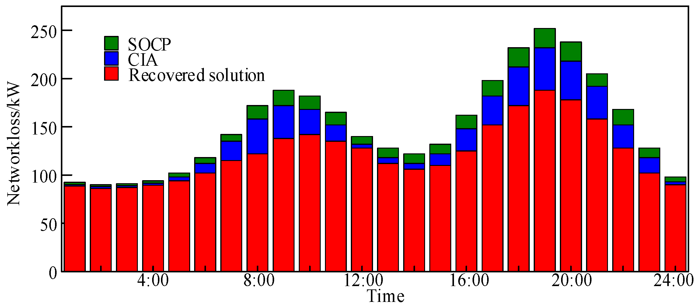
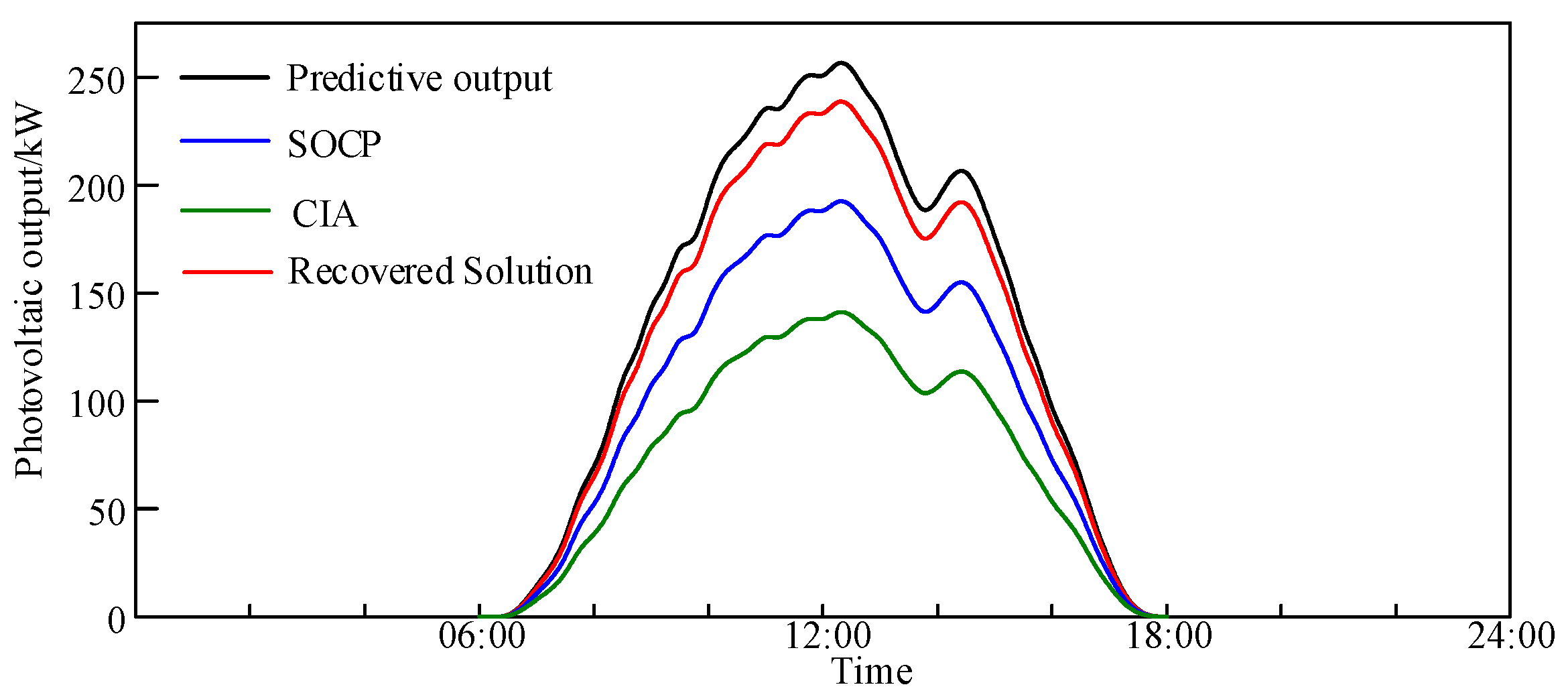
3.1. Branch Flow Model for Radial Distribution Networks

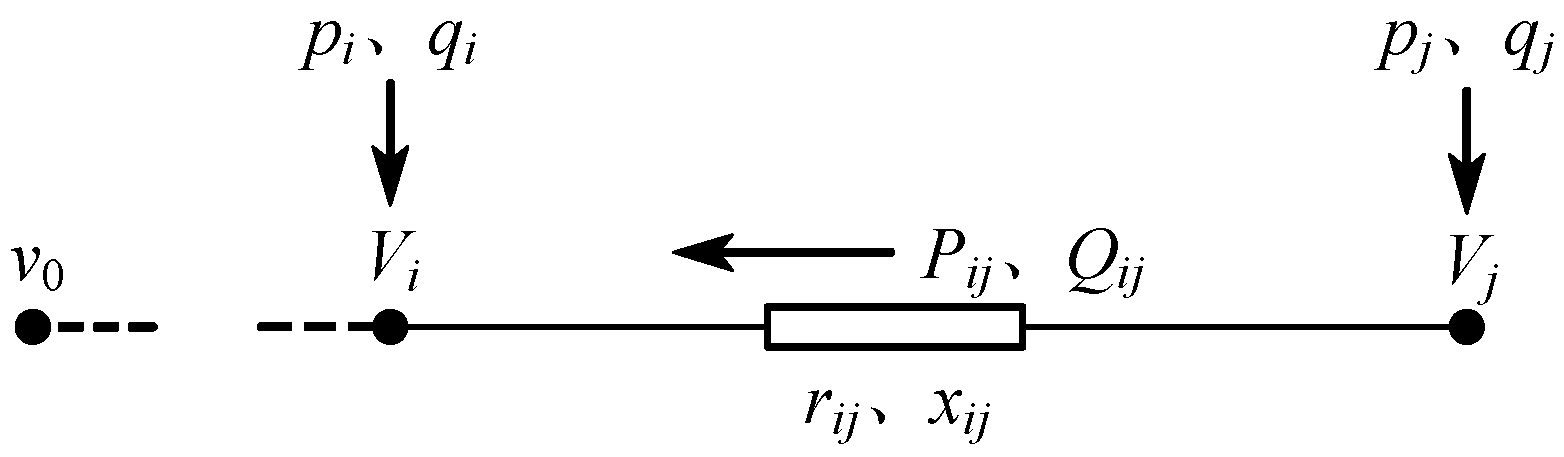
For the radial distribution network illustrated in Figure 2, the relationship between power flow and node voltages is described by the classical DistFlow Equation (1).

$$\left\{\begin{array}{l}{\upsilon }_i-{\upsilon }_j=2r_{ij}{P}_{ij}+2x_{ij}{Q}_{ij}-{\left|z_{ij}\right|}^2{l}_{ij}\\ P_{ij}=p_i+{\displaystyle \sum _{h:h\to i}\left(P_{hi}-r_{hi}{l}_{hi}\right)}\\ Q_{ij}=q_i+{\displaystyle \sum _{h:h\to i}\left(Q_{hi}-x_{hi}{l}_{hi}\right)}\\ l_{ij}{\upsilon }_i={P_{ij}}^2+{Q_{ij}}^2\end{array}\right.$$

(1)

Let ℝ, ℤ, and ℕ denote the sets of real numbers, integers, and natural numbers, respectively. The undirected graph G is composed of n + 1 nodes and n branches, where Ν and L represent the sets of nodes and branches, respectively. An undirected graph G is composed of n + 1 nodes and n branches. Let N be the set of nodes and L be the set of branches, defined as $G=\left\{N,L\right\}$, such that if nodes are interconnected, then $\left(i,j\right)\in L$. Let $B\in R^{(n+1)\times n}$ represent the incidence matrix of G, which associates the nodes in N with the branches in L. Let V_i be the voltage phasor at node i, and I_ij be the current phasor of branch $\left(i,j\right)\in L$, where ${\upsilon }_i={\left|V_i\right|}^2$,$lij={\left|I_{ij}\right|}^2$. P_ij and Q_ij denote the active and reactive power flowing from node i to node j, while p_i and q_i represent the net active and reactive power injected at node i, r_ij and x_ij denote the resistance and reactance of the branch, respectively, with $z_{ij}=r_{ij}+j{x}_{ij}$ representing the branch impedance.

3.2. Basic Principles of the Convex Inner Approximation Method

In the field of power system optimization, mathematical challenges are posed in solving the corresponding optimization models due to the inherent non-convex and nonlinear characteristics of DistFlow equations. The presence of nonlinear terms results in a non-convex geometric configuration of the feasible solution set. Such non-convexity may lead to multiple local optima, thereby causing conventional optimization algorithms to easily fall into local optimal traps and rendering convergence difficult to guarantee. By introducing a convex inner approximation (CIA) model, the feasible region is restricted to a convex subset of the original non-convex set while the essence of the physical constraints of the original problem is maintained. This ensures the feasibility of the solutions while improving computational efficiency.

Clearly, the non-convexity of the DistFlow model stems from the nonlinear nature of the line loss equality constraint in Equation (1). In the remainder of this section, a mathematical model of the radial network will be constructed to express the constrained variables as linear functions of nodal power injections and branch currents. Through this approach, the model can be decomposed into linear and nonlinear components. This will lay the foundation for bounding the nonlinear terms, thereby providing a convex inner approximation of the power flow equations. Based on the incidence matrix B of the radial network and referring to the method proposed in [28], Equation (1) is first expressed in a compact structural representation using matrices:

$$\left\{\begin{array}{l}\mathit{P}=\mathit{p}+\mathit{A}\mathit{P}-\mathit{A}\mathit{R}\mathit{l}\\ \mathit{Q}=\mathit{q}+\mathit{A}\mathit{Q}-\mathit{A}\mathit{X}\mathit{l}\end{array}\right.$$

(2)

In the expressions, $\mathit{P}=[P_{ij}]$, $\mathit{Q}=[Q_{ij}]$, $\mathit{p}=[p_i]$, $\mathit{q}=[q_i]$, $\mathit{R}=diag\left\{r_{ij}\right\}$, $\mathit{X}=diag\left\{x_{ij}\right\}$, $\mathit{l}=[l_{ij}]$, $\mathit{A}=[\begin{array}{cc}{\mathbf{0}}_n& {\mathit{I}}_n\end{array}]\mathit{B}-{\mathit{I}}_n$, $\left(i,j\right)\in L$, where I_n represents an identity matrix of order n, and 0_n denotes a column vector of zeros with length n.

By defining ${({\mathit{I}}_n-\mathit{A})}^{-1}$ as matrix C, ${({\mathit{I}}_n-\mathit{A})}^{-1}\mathit{AR}$ as matrix D_R, and ${({\mathit{I}}_n-\mathit{A})}^{-1}\mathit{AX}$ as matrix D_X, the following is obtained:

$$\left\{\begin{array}{l}\mathit{P}=\mathit{Cp}-{\mathit{D}}_R\mathit{l}\\ \mathit{Q}=\mathit{Cq}-{\mathit{D}}_X\mathit{l}\end{array}\right.$$

(3)

Defining ${\mathit{Z}}^2=diag\left\{{x_{ij}}^2\right\}$, $\mathit{V}=[{\upsilon }_i]$, ${\mathit{B}}_n=[\begin{array}{cc}{\mathbf{0}}_n& {\mathit{I}}_n\end{array}]\mathit{B}$, diag(B_n) = diag(2I_n − B_n) = 1_n, the recursive relationship between node voltages is expressed via the substation node V₀ with a fixed voltage as:

$${\mathit{C}}^{\top }[{\upsilon }_i-{\upsilon }_j]=\mathit{V}-{\upsilon }_0{\mathit{1}}_n$$

(4)

Substituting Equation (4) into Equation (1) yields:

$$\mathit{V}={\upsilon }_0{\mathit{1}}_n+2({\mathit{C}}^{\top }\mathit{RP}+{\mathit{C}}^{\top }\mathit{XQ})-{\mathit{C}}^{\top }{\mathit{Z}}^2\mathit{l}$$

(5)

By combining Equations (3) and (5), the relationship between the voltage and the injected active and reactive power is derived as:

$$\mathit{V}={\upsilon }_0{\mathit{1}}_n+{\mathit{M}}_p\mathit{p}+{\mathit{M}}_q\mathit{q}-\mathit{Hl}$$

(6)

In these equations, ${\mathit{M}}_p=2{\mathit{C}}^{\top }\mathit{RC}$, ${\mathit{M}}_q=2{\mathit{C}}^{\top }\mathit{XC}$, $\mathit{H}={\mathit{C}}^{\top }(2(R{\mathit{D}}_R+{\mathit{XD}}_X)+{\mathit{Z}}^2)$.

The non-negativity of Matrix H is a critical premise for the proposed CIA method. The validity of this assumption is rigorously justified as follows:

First, according to the definition of the network topology, Matrix A is inherently non-negative. Second, regarding Matrix C, it is observed that C⁻¹ possesses positive diagonal elements and non-positive off-diagonal elements, characterizing it as a Z-matrix. Since B_n is an upper triangular matrix with positive eigenvalues, C⁻¹ is identified as a non-singular M-matrix. According to the inverse-positive property of M-matrices, the inverse of an M-matrix is a non-negative matrix; thus, Matrix C is non-negative [30].

Consequently, since both A and C are non-negative, Matrix H remains non-negative regardless of whether the line impedance matrix X is non-negative (inductive), non-positive (capacitive/cables), or zero (resistive). This theoretical conclusion is further supported by numerical verification conducted on the IEEE 33-node system, where all elements of Matrix H were confirmed to be non-negative across all simulated scenarios.

It is worth noting that if this non-negativity condition were not met (e.g., in non-radial topologies), the convexity guarantee of the inner approximation would be violated, potentially resulting in infeasible solutions that exceed the original safety boundaries.

To address the nonlinearity in Equation (6), let l_max and l_min denote the upper and lower bounds of the current l, respectively. Consequently, the upper and lower bounds of the voltage V can be derived as follows:

$$\left\{\begin{array}{l}{\mathit{V}}^{+}={\upsilon }_0{\mathit{1}}_n+{\mathit{M}}_p\mathit{p}+{\mathit{M}}_q\mathit{q}-\mathit{H}{l}_{\min }\\ {\mathit{V}}^{-}={\upsilon }_0{\mathit{1}}_n+{\mathit{M}}_p\mathit{p}+{\mathit{M}}_q\mathit{q}-\mathit{H}{l}_{\max }\end{array}\right.$$

(7)

The initial operating point of the system is defined as $x_{ij}^0=col\{P_{ij}^0,Q_{ij}^0,{\upsilon }_j^0\}$, and the superscript 0 for other variables denotes their values at this initial operating point. For instance, $l_{ij}^0=l_{ij}(x_{ij}^0)$ represents the square of the branch current at the initial point.

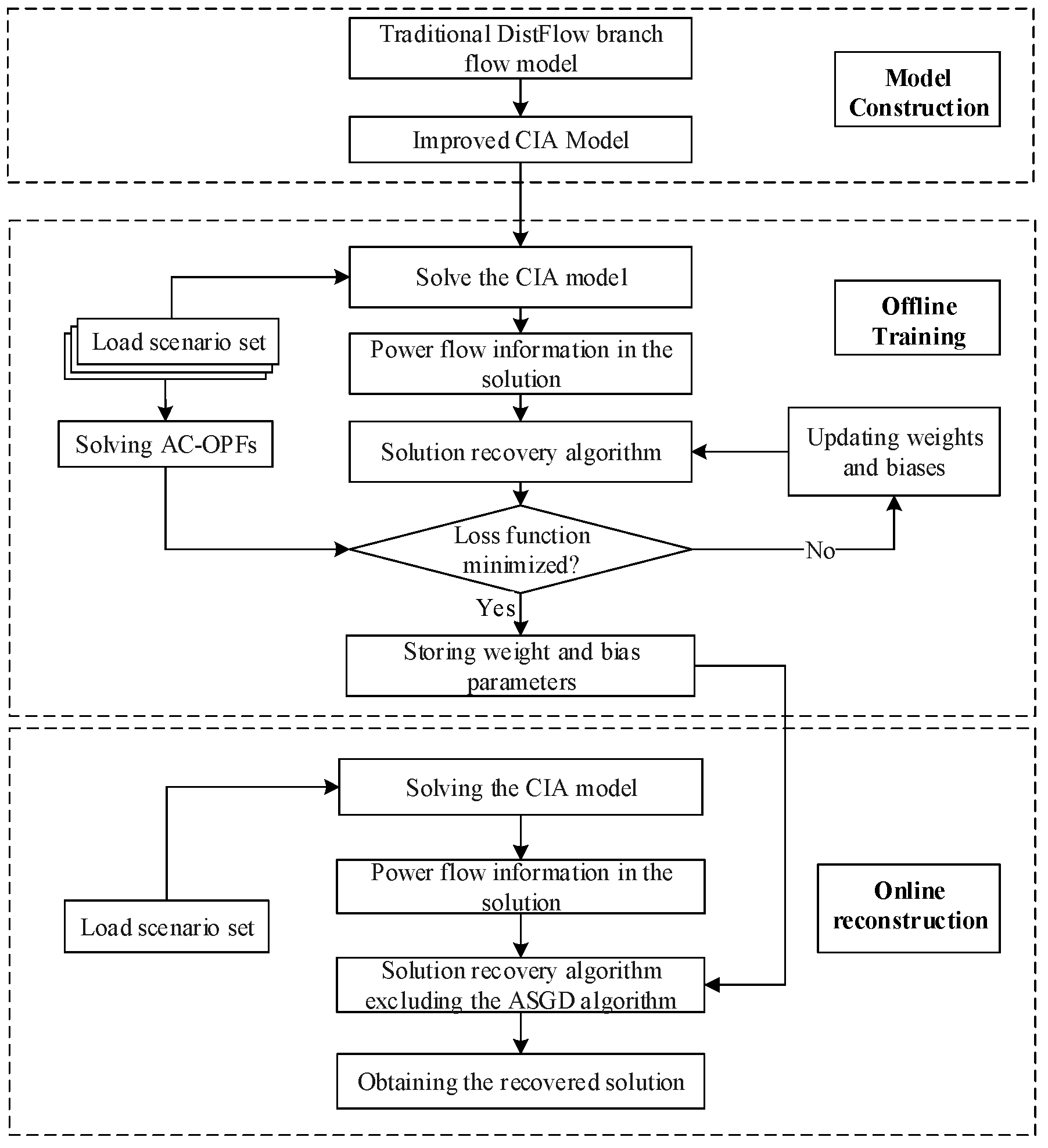
In general, the initial operating point is defined based on the forecasted net-demand values. However, a fixed operating point without iterative refinement (such as the convex-concave procedure) may lead to conservative estimates of the feasible region, particularly when the operating point deviates significantly from the optimal state. Yet, iterative optimization requires repeated solving of optimization problems, which poses computational limitations for real-time applications. Therefore, this paper adopts a unique strategy: the conservativeness introduced by a static initial point is accepted during the optimization stage and subsequently compensated for by the proposed solution recovery mechanism. As demonstrated in the simulation section, the trained recovery parameters effectively correct the deviations, ensuring both solution accuracy and online computational efficiency. Subsequently, an approximation can be derived via the second-order Taylor expansion formula as follows:

$$l_{ij}\approx l_{ij}^0+{\mathit{J}}_{ij}^{\top }{\mathsf{\delta }}_{ij}+{\displaystyle \frac{1}{2}}{\mathsf{\delta }}_{ij}^{\top }{\mathit{H}}_{e,ij}{\mathsf{\delta }}_{ij}$$

(8)

In the expressions, δ_ij, J_ij, and H_e,ij are defined as follows:

$${\mathsf{\delta }}_{ij}=\left[\begin{array}{l}{P}_{ij}-P_{ij}^0\\ Q_{ij}-Q_{ij}^0\\ {\upsilon }_j-{\upsilon }_j^0\end{array}\right], {\mathit{J}}_{ij}=\left[\begin{array}{c}{\displaystyle \frac{2P_{ij}^0}{{\upsilon }_i^0}}\\ {\displaystyle \frac{2Q_{ij}^0}{{\upsilon }_i^0}}\\ -{\displaystyle \frac{{(P_{ij}^0)}^2+{(Q_{ij}^0)}^2}{{({\upsilon }_i^0)}^2}}\end{array}\right], {\mathit{H}}_{e,ij}=\left[\begin{array}{ccc}\frac{2}{{\upsilon }_i^0}& 0& {\displaystyle \frac{-2P_{ij}^0}{{({\upsilon }_i^0)}^2}}\\ 0& {\displaystyle \frac{2}{{\upsilon }_i^0}}& {\displaystyle \frac{-2Q_{ij}^0}{{({\upsilon }_i^0)}^2}}\\ {\displaystyle \frac{-2P_{ij}^0}{{({\upsilon }_i^0)}^2}}& {\displaystyle \frac{-2Q_{ij}^0}{{({\upsilon }_i^0)}^2}}& 2{\displaystyle \frac{{(P_{ij}^0)}^2+{(Q_{ij}^0)}^2}{{({\upsilon }_i^0)}^3}}\end{array}\right].$$

Through bounding and scaling, l_max and l_min can be obtained as:

$$l_{ij}\approx l_{ij}^0+{\mathit{J}}_{ij}^{\top }{\mathsf{\delta }}_{ij}+{\displaystyle \frac{1}{2}}{\mathsf{\delta }}_{ij}^{\top }{\mathit{H}}_{e,ij}{\mathsf{\delta }}_{ij}\ge l_{ij}^0+{\mathit{J}}_{ij}^{\top }{\mathsf{\delta }}_{ij}=l_{\min ,ij}$$

(9)

$$\begin{array}{l}\left|l_{ij}\right|\approx \left|l_{ij}^0+{\mathit{J}}_{ij}^{\top }{\mathsf{\delta }}_{ij}+{\displaystyle \frac{1}{2}}{\mathsf{\delta }}_{ij}^{\top }{\mathit{H}}_{e,ij}{\mathsf{\delta }}_{ij}\right|\le \left|l_{ij}\right|+\left|{\mathit{J}}_{ij}^{\top }{\mathsf{\delta }}_{ij}\right|+\left|{\displaystyle \frac{1}{2}}{\mathsf{\delta }}_{ij}^{\top }{\mathit{H}}_{e,ij}{\mathsf{\delta }}_{ij}\right|\\ \le l_{ij}^0+\max \{2\left|{\mathit{J}}_{ij}^{\top }{\mathsf{\delta }}_{ij}\right|,\left|{\mathsf{\delta }}_{ij}^{\top }{\mathit{H}}_{e,ij}{\mathsf{\delta }}_{ij}\right|\}=l_{\max ,ij}\end{array}$$

(10)

As indicated in Equation (9), the calculated lower bound l_min,ij may mathematically assume negative values; however, from a physical perspective, l_min,ij is strictly constrained to be non-negative. Furthermore, an analysis of the expression for J_ij reveals that as the power flows $P_{ij}^0$ and $Q_{ij}^0$ approach zero (i.e., light load conditions), l_min,ij is effectively constrained to zero. This observation indicates that the tightness of the derived bounds is dependent on the operating conditions, and the resulting estimates generally exhibit a conservative nature. In fact, such conservatism is closely correlated with the selection of the initial operating point discussed previously.

Generally, the initial operating point is defined based on the forecasted net demand. However, a fixed operating point without iterative refinement—such as via the convex-concave procedure—may lead to conservative feasible region estimates, especially when the operating point deviates significantly from the optimal state. Nevertheless, iterative optimization requires repeatedly solving the optimization problem, which imposes computational limitations for real-time applications. Therefore, this paper adopts a distinct strategy: the conservatism resulting from a static initial point is accepted during the optimization stage and is subsequently compensated by the proposed solution recovery mechanism. As demonstrated in the simulation section, the trained recovery parameters effectively correct the deviations, ensuring both solution accuracy and online computational efficiency.

3.3. Optimal Distribution Network Scheduling Model Solution

Under the optimization framework of the new power system driven by the “Dual Carbon” goals, carbon emission constraint indicators have evolved into core policy variables and quantifiable control tools in the energy transition process [31]. As a key parameter characterizing the energy efficiency of the transmission network, active power loss exhibits a significant positive correlation with carbon emission intensity. In light of the fact that the low-carbon attribute of distribution network dispatch is primarily reflected in reducing energy losses and enabling clean energy substitution, this paper considers the minimization of active power loss and the maximization of distributed generation (DG) output as physical equivalent proxy variables for reducing redundant carbon emissions and offsetting high-carbon power generation, respectively. Through multi-objective collaborative optimization, the operational low-carbon performance is enhanced while improving system efficiency. Simultaneously, the rising wind and solar curtailment rates—triggered by the volatility of renewable energy output and the insufficiency of grid regulation capabilities—highlight the urgent need to enhance the accommodation efficiency of distributed generations (DG) [32]. Finally, as a traditional rigid constraint for the steady-state secure operation of power systems, the Voltage Deviation Index remains a critical component of the power system security domain boundary criteria that cannot be neglected [33]. Based on these considerations and with reference to [29], a multi-objective collaborative optimization model is constructed in this study. The objective functions include:

(1)

Minimization of System Active Power Loss:

$$f_1=\min {\displaystyle \sum _{t=1}^T{\displaystyle \sum _{i=1}^n{\displaystyle \sum _{j=1}^n{G}_{ij}}}}({\upsilon }_i+{\upsilon }_j-2V_i{V}_j\cos {\theta }_{ij})\Delta t$$

(11)

In this expression, T denotes the total number of observation periods; G_ij is the conductance of line ij; V_i and V_j are the voltage magnitudes at nodes i and j, respectively; Δt represents the time interval between two observation points; and θ_ij is the phase angle difference between nodes i and j.

(2)

Minimization of the Absolute Value of Node Voltage Deviation:

$$f_2=\min {\displaystyle \sum _{i=1}^N\left|V_{i,t}-V_{i,ref}\right|}$$

(12)

Nodes at line terminals or those where state variables are integrated are defined as weak nodes of the system. The optimization objective function for conventional nodes, excluding these weak nodes, is shown above. Here, N represents the number of conventional nodes; V_i,t and V_i,ref denote the voltage magnitude and the reference voltage value of the i-th node at time t, respectively.

(3)

Maximization of DG Output:

$$f_3=\min (-{\displaystyle \sum _{t=1}^T{\displaystyle \sum _{i=1}^{N_G}\left|P_{g,i}^t\right|}})$$

(13)

In this expression, N_G is the number of DG in the system, and $P_{g,i}^t$ represents the output of the DG at node i at time t.

Since the three indicators mentioned above belong to different dimensions, normalization is required. The final objective function is obtained by weighting these indicators using the Analytic Hierarchy Process (AHP):

$$f=\alpha f_1/f_{10}+\beta f_2/f_{20}+\gamma f_3/f_{30}$$

(14)

where α, β, and γ are the corresponding weight coefficients determined by AHP, satisfying α + β + γ = 1. Considering the rigid requirements for the safe operation of distribution networks, the highest priority is assigned to the voltage deviation index. The constructed AHP judgment matrix and the calculated weights are presented in

Table 1. The judgment matrix and weights of objectives.

Objectives	f1 (Loss)	f2 (Volt)	f3 (DG)	Weights
f1 (Loss)	1	1/2	2	0.297
f2 (Volt)	2	1	3	0.540
f3 (DG)	1/2	1/3	1	0.163

. The calculation yields a maximum eigenvalue λ_max = 3.009, a consistency index CI = 0.0045, and a consistency ratio CR = 0.008 (<0.1). These results verify that the judgment matrix satisfies the consistency constraint and the weight allocation is rational.

f₁₀ and f₂₀ are the benchmark values for active power loss and voltage deviation, respectively, calculated from the initial operating state of the system (i.e., the baseline scenario before any control variables are activated), serving to eliminate differences in dimensionality; f₃₀ represents the total installed capacity of distributed generation within the system, which is used as a dimensionless reference upper limit.

For the weak nodes of the system, a penalty is applied to the portions exceeding the limits. The objective function in this case is:

$$\min F=f+k{\displaystyle \sum _{i=1}^{N_{weak}}{(V_{i,t}-V_{i.ref})}^2}$$

(15)

where N_weak is the number of weak nodes and k is the penalty coefficient. A parameter sensitivity analysis was conducted to determine the optimal value of the penalty coefficient k. The results indicate that when k < 100, the penalty is insufficient, and voltage violations persist at certain weak nodes. As k increases within the range of [100, 1000], voltage violations decrease rapidly and are eventually eliminated. When k > 1000, the optimization results stabilize; further increasing k yields negligible improvements but raises the risk of numerical oscillation during the solution process. Therefore, balancing constraint strictness and convergence stability, k is set to 1000 in this study.

The decision variables selected in this paper include renewable DG represented by wind and solar power, stable-output DG represented by micro-gas turbines, and Static VAR Compensators (SVCs) and switchable capacitor banks used for system voltage compensation. The constraints consist of the CIA modeling constraints with reference to [28], supplemented by conventional constraints related to the decision variables.

4. Restoration of Feasible AC Power Flow Solutions

4.1. Principles of the Feasibility Restoration Algorithm

This section employs the mathematical mechanism of a typical state estimation algorithm to achieve the restoration of feasible solutions. In this algorithm, the voltage phasors, injection powers, and line transmission powers derived from the CIA solution are analogous to measurement noise, with the corresponding analogy detailed in

Table 2. Analogy between the Proposed Algorithm and State Estimation.

Proposed Algorithm	State Estimation
Solutions from CIA model	Measurements from physical sensors
Inconsistencies in CIA solutions	Noise from physical sensors
Weight parameters	Variance of the measurement noise
Bias parameters	-

. The distinction lies in the fact that these variables do not depend on actual physical measurements; instead, the methodology for handling inconsistencies among measurement noises in state estimation is employed to identify voltage phasors, power injections, and line flows that approximate the CIA solution as closely as possible. Weighting and bias parameters associated with the output quantities of the CIA solution are utilized by the algorithm to quantify systematic and random errors.

To obtain voltage magnitudes and phase angles (denoted as x) that are as close as possible to z, the voltage phasors, injected powers, and line power flow information obtained from the CIA solution are first represented by a vector z of length m. Subsequently, a model error bias parameter b is defined. Unlike in conventional state estimation algorithms, the bias regarding z may manifest as a consistent overestimation or underestimation of the true values of certain quantities. An error parameter e is then defined to capture systematic random errors. Finally, the AC power flow model is represented by h(x), which relates x to z while accounting for the bias b:

$${\mathit{z}}_i+{\mathit{b}}_i=h_i(\mathit{x})+{\mathit{e}}_i,i=1,\dots ,m$$

(16)

where V denotes voltage phasors; P and Q represent active and reactive power injections, respectively; P^f and Q^f signify the active and reactive power flows on the lines; and θ denotes the voltage phase angle, $h(\mathit{x})={[\mathit{V}{(\mathit{x})}^{\mathrm{{\rm T}}}\mathit{P}{(\mathit{x})}^{\mathrm{{\rm T}}}\mathit{Q}{(\mathit{x})}^{\mathrm{{\rm T}}}{\mathit{P}}^f{(\mathit{x})}^{\top }{\mathit{Q}}^f{(\mathit{x})}^{\top }\mathsf{\theta }{(\mathit{x})}^{\top }]}^{\top }$. The first and last terms of h(x) are derived from identities, while the remaining terms are obtained through classical OPF formulations.

To address the error e representing systematic random fluctuations, the weighted least squares method from state estimation is adopted. A cost function is designed to represent the inconsistency between the CIA solution and the optimal OPF solution, and an appropriate x is selected to minimize this cost function. The error e is weighted using a specific diagonal matrix Σ, where the weighting parameters are related to the solution obtained via the CIA algorithm:

$$\min G(\mathit{x})={\mathit{e}}^{\top }\mathsf{\Sigma }\mathit{e}$$

(17)

In state estimation algorithms, Σ represents the covariance matrix of sensor noise. In this study, this value is calculated based on the Adaptive Stochastic Gradient Descent (ASGD) method [34]. It is acknowledged that the approximation errors arising from CIA are structural and inherently non-Gaussian. However, the proposed framework explicitly addresses this by introducing the learnable bias parameter b to capture the systematic, non-zero mean deviations caused by convexification. Consequently, the remaining residual component e can be approximated as zero-mean random noise. By employing the Weighted Least Squares (WLS) formulation, the algorithm effectively minimizes the L₂ norm of these residuals. Furthermore, the adaptive weighting matrix Σ compensates for the potential heteroscedasticity of the errors, ensuring that the WLS approach remains robust and computationally efficient for solving the restoration problem via Newton-type methods.

The stationary point of Equation (17) can be obtained as follows:

$$g(\mathit{x})={\displaystyle \frac{\partial G(\mathit{x})}{\partial \mathit{x}}}=-J{(\mathit{x})}^{\top }\mathsf{\Sigma }(\mathit{z}+\mathit{b}-h(\mathit{x}))=0$$

(18)

where J(x) denotes the Jacobian matrix of the AC power flow formulation h(x) ${\displaystyle \frac{\partial h(\mathit{x})}{\partial \mathit{x}}}$. At the k-th iteration, the following equality holds:

$$\left\{\begin{array}{l}D(\mathit{x})={\displaystyle \frac{\partial g(\mathit{x})}{\partial \mathit{x}}}={J(\mathit{x})}^{\top }\mathsf{\Sigma }J(\mathit{x})\\ {\mathit{x}}^{(k+1)}={\mathit{x}}^{(k)}-{(D(\mathit{x}))}^{-1}g(\mathit{x})\end{array}\right.$$

(19)

The Newton-Raphson method is employed to iteratively solve Equation (18), and the corresponding flowchart is illustrated in Figure 3. The Newton-Raphson method is employed to solve Equation (18), as illustrated in Figure 3. The convergence of the iteration is determined by the criterion $‖\Delta x^{(k)}‖\le \epsilon$. To ensure numerical stability, the Hessian approximation D(x) is monitored, and the ASGD-based dynamic adjustment of Σ helps prevent ill-conditioning during the optimization process. While the CIA solution typically provides a high-quality initial point x⁽⁰⁾, the algorithm’s robustness is further evaluated using a flat start. It is observed that while poor initialization may increase the number of iterations, the algorithm consistently converges to a feasible AC solution x_R unless the system is operating near its physical stability limits.

The computational complexity of the proposed recovery algorithm is primarily governed by the formation and factorization of the Hessian-like matrix D(x) in each Newton-Raphson iteration. For a power system with n buses, the construction of the Jacobian matrix J(x) and the matrix multiplication $J{(\mathit{x})}^{\mathrm{T}}\mathsf{\Sigma }J(\mathit{x})$ have a complexity of O(n) by exploiting the sparsity of the network topology. The solution of the linear system in Equation (19) typically requires O(n^1.2~n^1.5) operations when sparse LU decomposition or similar techniques are employed. Since the CIA solution provides a high-quality initial point, the algorithm typically reaches convergence within a small, constant number of iterations (e.g., 3–5), ensuring that the overall computational burden remains scalable for large-scale power grids.

4.2. Parameter Optimization Based on the ASGD Algorithm

To better utilize the optimization algorithm mentioned in the previous section, the selection of the weighting parameters Σ and bias parameters b is of critical importance. Specifically, corresponding to the measurement vector z of length m, the weighting parameter Σ is defined as a diagonal matrix of dimension m × m, while the bias parameter b is formulated as a vector of dimension m × 1. Inspired by machine learning algorithms, and in consideration of the ASGD algorithm’s ability—due to its mechanism for dynamically adjusting learning rates—to stably handle the stochastic non-convex loss functions in optimal power flow problems, its superiority over traditional SGD and second-order optimization methods in terms of computational efficiency and accuracy, and its particular suitability for processing large-scale distribution network datasets, this paper employs the ASGD algorithm to train the model for parameter optimization.

The detailed procedure is depicted in Figure 4.

Initially, the initial weighting parameters Σ^st, b^st, batch size, maximum number of iterations, and ASGD parameters are input, and a series of load scenario schemes are created. For each load scenario, the actual solutions and the CIA algorithmic solutions are calculated in parallel, with the results stored in ${\mathit{x}}_{\mathrm{AC}}^{(i)}$ and z⁽ⁱ⁾, respectively. Subsequently, for each scenario, the information from the CIA solution is utilized alongside the algorithm shown in Figure 3 to obtain the restored feasible AC solution ${\mathit{x}}_{\mathrm{R}}^{(i)}$. Finally, with the objective of minimizing the loss function, the weighting and bias parameters are iteratively updated based on the differences between the ground-truth solutions and the optimized solutions, as well as their respective partial derivatives. The process is terminated once the maximum number of iterations is reached, and the optimal weighting and bias parameters (Σ^opt and b^opt) are returned as the output.

The sensitivities of the optimized solution x_R with respect to Σ and b are required by the ASGD algorithm ${\displaystyle \frac{\partial {\mathit{x}}_R}{\partial \mathsf{\Sigma }}}$, ${\displaystyle \frac{\partial {\mathit{x}}_R}{\partial \mathit{b}}}$:

$$\begin{array}{l}{\displaystyle \frac{vec(\partial {\mathit{x}}_R)}{vec(\partial \mathsf{\Sigma })}}=((\mathit{z}+\mathit{b}-h(\mathit{x}))-{((J(\mathit{x}){J(\mathit{x})}^{\top }\mathsf{\Sigma }J(\mathit{x}))}^{-1}\times \\ {J(\mathit{x})}^{\top }\mathsf{\Sigma }(\mathit{z}+\mathit{b}-h(\mathit{x}))))\otimes {({({J(\mathit{x})}^{\top }\mathsf{\Sigma }J(\mathit{x}))}^{-1}{J(\mathit{x})}^{\top })}^{\top }\end{array}$$

(20)

$${\displaystyle \frac{\partial {\mathit{x}}_R}{\partial \mathit{b}}}={(J{(\mathit{x})}^{\top }\mathsf{\Sigma }J(\mathit{x}))}^{-1}J{(\mathit{x})}^{\top }$$

(21)

where ⊗ denotes the Kronecker product and vec ( ) represents the vectorization of a matrix.

To evaluate the accuracy of the obtained optimized solution, a loss function must be defined to quantify the deviation from the ground-truth solution. Following the conventional approach for training ML (Machine Learning) models, the sum of squares of the differences between the voltage phasors of the optimized solution x_R and the ground-truth solution x_AC is defined as the loss function. To this end, new matrix vectors ${\mathit{X}}_R={[{x_R}^{(1)\top },{x_R}^{(2)\top },\dots ,{x_R}^{(S)\top }]}^{\top }$ and ${\mathit{X}}_{AC}={[{x_{AC}}^{(1)\top },{x_{AC}}^{(2)\top },\dots ,{x_{AC}}^{(S)\top }]}^{\top }$ are introduced, where S is the total number of scenarios. ${\mathit{x}}_{\mathrm{R}}^{(i)}$ and ${\mathit{x}}_{\mathrm{AC}}^{(i)}$ represent the vectors of voltage magnitudes and phase angles for all nodes in the network corresponding to the optimized OPF solution and the actual OPF solution for the i-th sampled load scenario. The loss function is then normalized based on the system size. Furthermore, to prevent overfitting, a regularization term is introduced, where λ is the regularization coefficient used to balance the fitting accuracy and model complexity. The final loss function can be expressed as:

$$F(\mathsf{\Sigma },\mathit{b})={\displaystyle \frac{1}{n}}{\displaystyle \sum _{i=1}^n{‖{\mathit{x}}_{\mathrm{R}}(\mathsf{\Sigma },\mathit{b})-{\mathit{x}}_{\mathrm{AC}}‖}_2^2}+\lambda ({‖\mathsf{\Sigma }‖}_F^2+{‖b‖}_2^2)$$

(22)

Parameter optimization is performed by the algorithm through the calculation of gradients of the loss function with respect to the weights and biases (denoted as q^var and q^bias, respectively) for parameter updates:

$$\left\{\begin{array}{l}{\mathit{q}}^{\mathrm{var}}={{\displaystyle \frac{2}{n}}{\displaystyle \sum _{i=1}^S\left.\frac{\partial {{\mathit{x}}_R}^{(i)}}{\partial \mathsf{\Sigma }}\right|}}_{{x_R}^{(i)}}({x_R}^{(i)}(\mathsf{\Sigma },\mathit{b})-{{\mathit{x}}_{AC}}^{(i)})\\ {\mathit{q}}^{\mathrm{bias}}={\displaystyle \frac{2}{n}}{{\displaystyle \sum _{i=1}^S\left.\frac{\partial {{\mathit{x}}_R}^{(i)}}{\partial \mathit{b}}\right|}}_{{x_R}^{(i)}}({{\mathit{x}}_R}^{(i)}(\mathsf{\Sigma },\mathit{b})-{{\mathit{x}}_{AC}}^{(i)})\end{array}\right.$$

(23)

Among the various versions of ASGD, the Adam algorithm is selected for the solution process in this study. The Adam algorithm is commonly utilized in machine learning models and involves the steps shown in Equation (24) during each iteration. In these expressions, m and τ represent the first and second moments of the gradient at the k-th iteration, respectively; η is the learning rate (step size); β₁ and β₂ are the exponential decay hyperparameters for the first and second moments; and ε is an infinitesimal constant.

The hyperparameters were selected based on standard industry recommendations and fine-tuned according to the model’s training characteristics. Specifically, the initial learning rate η is set to 0.001; the exponential decay rates for the moment estimates are set to β₁ = 0.9 and β₂ = 0.999; the batch size is selected as 128 to balance sample size and training efficiency; and ε is fixed at 10⁻⁸ to prevent numerical instability. To evaluate the robustness of this selection, a sensitivity analysis was performed. The results indicate that the algorithm maintains stable convergence even when the learning rate varies within the range of [10⁻⁴, 10⁻²], demonstrating the insensitivity of the proposed method to minor hyperparameter perturbations. Furthermore, compared to simpler strategies such as standard Stochastic Gradient Descent (SGD) with fixed learning rates, the adopted Adam algorithm exhibited significantly faster convergence speeds and lower final loss values in our comparative tests.

The update process for parameter b is analogous to that shown in Equation (23).

$$\left\{\begin{array}{l}\mathsf{\Gamma }={\displaystyle \frac{\mathsf{\tau }}{1-{{\beta }_2}^k}}\\ \mathsf{\Sigma }=\mathsf{\Sigma }-\eta {\displaystyle \frac{\hat{\mathit{m}}}{\sqrt{\mathsf{\Gamma }}+\epsilon }}\\ \mathit{m}={\beta }_1\mathit{m}+(1-{\beta }_1)\mathit{q}\\ \mathsf{\tau }={\beta }_2\mathsf{\tau }+(1-{\beta }_2){(\mathit{q})}^2\\ \hat{\mathit{m}}={\displaystyle \frac{\mathit{m}}{1-{{\beta }_1}^k}}\end{array}\right.$$

(24)

5. Case Study and Validation

To verify the effectiveness of the proposed method, simulation tests were performed on the MATLAB-Yalmip platform by invoking the CPLEX solver. Meanwhile, the commercial solver MOSEK was adopted to obtain the optimal solutions for the original problem, which served as benchmark data for the training and testing sets. The experimental environment was configured as follows: The hardware included a Lenovo computer (manufactured by Lenovo Group Ltd., Beijing, China) equipped with an Intel Core i7-8750H processor (2.20 GHz clock speed) running on the Windows 10 operating system, while the software environment comprised MATLAB R2022a and Yalmip (version 20200116). All experiments were conducted at Jiangsu University, Zhenjiang, Jiangsu Province, China.

5.1. Simulation of the IEEE 33-Node System

5.1.1. Case Description

The IEEE 33-node radial distribution system was selected as the subject of simulation and analysis. This system consists of 32 branches with a voltage level of 12.66 kV. The total active and reactive power loads are 3715 kW and 2547 kvar, respectively. The quantities, capacities, and integration locations of devices such as Distributed Generation (DG), Static Var Compensators (SVC), Capacitor Banks (CB), and Energy Storage Systems (ESS) are summarized in

Table 3. Parameters of Each decision variable of IEEE33 bus systems.

Type	Name	Number of Units	Grid-Connected Node	Active Power/MW	Reactive Power/MVar
DG	Photovoltaic Cells	2	10, 24	0~0.5	-
DG	Wind Turbine Generator	2	17, 32	0~0.5	-
DG	Micro Gas Turbine	1	13	0~0.3	0~0.3
ESS	Battery Energy Storage	2	16, 32	0~0.5	0~0.5
SVC	Static Var Compensator	1	25	-	0~1.0
CB	Capacitor Bank	10	22	-	0~0.5

.

Given the limited geographical area covered by the distribution network, the typical summer daily curves of a city in East China [29] were utilized for the time-series profiles of the load, photovoltaic (PV) generation, and wind turbines (WT).

5.1.2. Analysis of ASGD Parameter Optimization Results

To obtain reasonably accurate parameters, a dataset containing 1000 scenarios was constructed based on the IEEE 33-node system, with 800 scenarios used for model training and 200 for performance testing. The diversity of the dataset was ensured through the following methods: First, load scenarios were generated by applying multiplicative perturbations to typical historical regional loads. Let the base load be P_base; the actual load P_act is expressed as $P_{act}=P_{base}(1+\epsilon )$, where the perturbation factor ε follows a normal distribution with a mean of 0 and a standard deviation of 0.1. Second, the integration locations and penetration levels (up to 60%) of distributed generators (DGs) were treated as key variables to simulate fluctuations caused by high shares of renewable energy integration. This construction approach ensures that the training set can cover the nonlinear characteristics of the distribution network under various operating conditions.

Due to space constraints, the analysis focuses on the weighting parameters, which exert a more significant impact on the results. Heatmaps representing the final mapping weight parameters (i.e., the diagonal elements of the Σ matrix) for node voltage, active power, and reactive power are presented in Figure 5, Figure 6 and Figure 7, respectively.

In these heatmaps, color blocks closer to blue indicate higher weights, while those closer to red indicate lower weights. It can be observed that specific physical variables are assigned significantly higher weights than others. For instance, compared with Figure 6 and Figure 7, Figure 5 contains a greater number of high-impact weight nodes, suggesting that voltage magnitude parameters play a dominant regulatory role in the restoration process of machine learning-driven relaxed solutions. Regarding each physical quantity, higher weights are observed for the voltage magnitude variables near Node 17, the active power variables at Nodes 10 and 24, and the reactive power variable at Node 25. This indicates that the physical quantities at these nodes possess superior statistical properties for restoring the actual Optimal Power Flow (OPF) solutions. Larger weights signify higher reliability of the corresponding variables during the reconstruction of AC feasible solutions by the algorithm.

5.1.3. Comparative Analysis of Restored Solutions and Other Methods

Since the objective functions of this study include the optimization of active power loss, voltage deviation, and DG output, a comparative analysis was performed based on these three indicators.

Figure 8 illustrates the dynamic distribution characteristics of the system’s active power loss over the entire period. The curves obtained by the three algorithms exhibit similar trends: the power loss remains at a low level from 00:00 to 07:00, followed by an increase with local peaks at 10:00 and 14:00. After 17:00, a sharp increase in power loss is observed, reaching the daily maximum around 21:00 before gradually receding to nighttime levels. This pattern is highly consistent with typical daily load curves. The improved CIA algorithm effectively reduces the overall active power loss compared to the SOCP algorithm, and the restoration algorithm achieves a further reduction. Notably, the optimization effect of the restoration algorithm is more pronounced when the system is under heavy load conditions, such as around 20:00.

The time section at 12:00 (midday), when PV output is at its maximum, was selected to investigate the voltage distribution. As shown in Figure 9, significant voltage fluctuations are observed. Under SOCP optimization, voltage violations occur at nodes near the branch ends. After CIA optimization, the voltage fluctuations no longer exceed the limits, and the magnitude of fluctuation is reduced. The restoration solution demonstrates superior optimization performance compared to the CIA solution, yielding a smoother voltage profile and significant peak optimization at weak nodes.

To verify the performance of the algorithm during the heavy load phase, simulations were conducted for the heavy load period (20:00–22:00) at weak Node 17. The results, shown in Figure 10, indicate that the voltage fluctuation range of CIA is reduced by 23% compared to SOCP. At 20:50, the voltage recovers to 0.979 (0.6% higher than that of SOCP), validating the role of integer constraint modeling in mitigating voltage droop. The voltage of the restored solution is maintained above 0.98 consistently, with a maximum deviation of only 2.0% (compared to 3.0% for SOCP). Furthermore, the voltage recovers rapidly to 0.988 after 21:40 (20 min earlier than SOCP/CIA), reflecting the strong compensation capability of the method’s dynamic correction mechanism for relaxation biases.

While the CIA optimization method significantly restricts the output of PV and WT to prevent voltage limit violations—resulting in a conservative dispatchable capacity—the restoration solution optimizes this conservativeness.

Figure 11 provides a comparison of the optimized DG output at Nodes 10 and 17.

Table 4. Comparison of performance indicators of three optimization methods.

Optimization Method	RMSE (kW)	MAPE (%)	Maximum Positive Deviation	Maximum Negative Deviation
SOCP	34.72	16.8	3.22	67.84
CIA	39.15	18.3	0.32	73.84
Recovery Algorithm	12.46	6.2	0.38	30.02

summarizes the statistical performance of the optimization methods in terms of Root Mean Square Error (RMSE) and Mean Absolute Percentage Error (MAPE). Among the three optimization algorithms, the AC power flow feasible solution restoration algorithm aligns most closely with the predicted DG output, successfully addressing the issue of overly conservative DG output inherent in the CIA method.

5.2. Simulation of the IEEE 69-Node System

To verify the applicability of the proposed methodology in larger-scale systems, the IEEE 69-node distribution system is further utilized for simulation. The system topology and parameters are based on those provided in reference [29]. The capacities and integration locations of Distributed Generation (DG) and other related devices are summarized in

Table 5. Parameters of Each decision variable of IEEE 69 bus systems.

Type	Nmae	Number of Units	Grid-Connected Node	Active Power/MW	Reactive Power/MVar
DG	Photovoltaic Cells	2	26, 35	0~0.5	-
DG	Wind Turbine Generator	2	56, 69	0~0.5	-
DG	Micro Gas Turbine	1	17	0~0.3	0~0.3
ESS	Battery Energy Storage	2	18, 27	0~0.5	0~0.5
SVC	Static Var Compensator	2	10, 52	-	0~1.0
CB	Capacitor Bank	10	10, 17, 27, 35, 39, 54, 69	-	0~0.5

.

In this configuration, two units each of photovoltaic (PV) cells, wind turbines (WT), battery energy storage systems (BESS), and static var compensators (SVC) are installed at two distinct nodes. A single micro-gas turbine (MT) is integrated at Node 17, while ten groups of capacitor banks (CB) are installed at each of the seven designated nodes.

The power loss at weak nodes of the IEEE 69-node system across different time periods is presented in Figure 12. It is observed that the lowest active power loss is achieved under the feasible solution restoration model. The improvement is particularly significant during heavy load periods, specifically around 11:00 and 20:00.

The voltage distribution of the entire network at 12:00 after optimization is illustrated in Figure 13. It can be seen that while voltage violations present in the SOCP method are eliminated by the CIA method, a smoother overall voltage profile with reduced fluctuations is obtained by the restoration model.

Figure 14 displays the 24 h PV output at Node 26. It is noted that the PV output obtained by the CIA algorithm is lower than that of the SOCP algorithm, representing the lowest output among the evaluated methods. This reflects the inherent conservativeness of the CIA method regarding DG resource dispatch. In contrast, the PV output values generated by the restoration model are positioned between the predicted output and the SOCP results, thereby significantly enhancing the utilization rate of PV-based DG within the system.

Table 6. Comparison of indexes between three methods in IEEE 69-Node System.

Method	Average Voltage Deviation	Power Loss/(kW·h)	DG Utilization Rate	Solution Time
SOCP	0.719	3657.9	77.16%	49.040 s
CIA	0.623	3163.1	67.14%	24.156 s
Recovery Algorithm	0.475	2972.4	83.59%	27.627 s

presents the performance metrics of three different optimization methods over a 24 h period in the IEEE 69-bus system. Taking the SOCP algorithm data as the baseline, the solution recovery algorithm reduces the average voltage deviation by 33.9%, decreases power loss by 18.7%, and shortens the online recovery solution time by 42.6%. Relative to the CIA algorithm data, the solution recovery algorithm improves the DG utilization rate by 24.5%.

These results demonstrate that the CIA method outperforms the traditional SOCP method in terms of voltage deviation, active power loss, and computational efficiency, albeit at the cost of reduced DG utilization. In contrast, the proposed restoration method surpasses the CIA method in voltage deviation, active power loss, and DG utilization. While its solution time is slightly higher than that of the CIA method, it remains significantly lower than that of the traditional SOCP model.

5.3. Simulation of the IEEE 118-Node System

To further verify the robustness of the proposed method within a larger-scale network and under varying seasonal load characteristics, the IEEE 118-node test system is employed for extended simulation verification. The algorithm consistently converges within 3–5 iterations even for the 118-node system, demonstrating stable convergence behavior. The objective functions and boundary conditions remain consistent with those defined in the previous section. The detailed topology of the IEEE 118-node distribution system is illustrated in Figure 15.

The voltage distribution across the entire network at 12:00, optimized by different methods, is depicted in Figure 16. It is observed that severe voltage limit violations occur at the weak nodes of the system when the SOCP method is applied. In contrast, these violations are effectively eliminated by the CIA method, while the voltage profile obtained through the proposed solution recovery model exhibits the minimum overall fluctuation.

A comparison of network losses for the IEEE 118-node system is presented in Figure 17. It can be observed that during high-load periods, the reduction in network losses achieved by the solution recovery algorithm remains most significant, particularly at the heavy-load nodes of the system.

The 24 h photovoltaic (PV) power output under various optimization algorithms and predicted values is provided in Figure 18. Compared to the characteristics shown in Figure 14, the PV output here features lower peak values, more pronounced fluctuations, and shorter durations of effective power generation; this is attributed to the simulation being conducted under a winter scenario. It is noted that the PV output associated with the CIA algorithm is lower than that of the SOCP algorithm, remaining the lowest among all methods, which further substantiates its conservatism regarding distributed generation (DG) resource scheduling. Conversely, the PV output derived from the recovery model is situated between the predicted output and the SOCP results, thereby significantly enhancing the system’s utilization rate of PV-based DG.

Table 7. Comparison of indexes between three methods in IEEE 118-Node System.

Method	Average Voltage Deviation	Power Loss/(MW·h)	DG Utilization Rate	Solution Time
SOCP	0.709	40.1	73.23%	142.852 s
CIA	0.644	37.7	66.05%	112.087 s
Recovery Algorithm	0.549	30.2	86.19%	77.991 s

provides a comprehensive performance comparison of the three optimization strategies within the IEEE 118-node system.

The performance metrics for the three optimization methods over a 24 h period in the IEEE 118-node system are summarized in Table 7. With the SOCP algorithm serving as the benchmark, the average voltage deviation and power losses of the proposed solution recovery algorithm are reduced by 22.6% and 24.7%, respectively, while the online solution time is shortened by 45.4%. Furthermore, taking the CIA algorithm as the benchmark, the DG utilization rate of the solution recovery algorithm is improved by 30.5%. As a typical representation of a large-scale distribution network, the simulation results of this system demonstrate that the proposed solution recovery algorithm can effectively mitigate network losses and voltage deviations while simultaneously enhancing DG utilization and computational efficiency.

6. Conclusions

In this paper, a feasible solution restoration strategy for AC power flow in active distribution networks is proposed, which accounts for the conservativeness of the feasible region inherent in the improved Convex Inner Approximation (CIA) method. Through simulation validation and analysis, the following conclusions are drawn:

(1)

In radial active distribution networks with a high penetration of renewable energy, modeling based on the improved CIA method provides a more universal application premise compared to traditional relaxation methods represented by SOCP. Furthermore, higher computational efficiency and solution speeds are achieved through CIA modeling.

(2)

Compared with SOCP and CIA, the restoration model based on the ASGD algorithm better suppresses voltage fluctuations across the entire network and eliminates local voltage limit violations. Meanwhile, system power losses are significantly reduced during heavy-load periods at weak nodes.

(3)

To address the conservative DG output issue of the CIA method, the solution recovery model, inspired by machine learning techniques, enhances DG utilization by training and adjusting key nodal parameters in voltage and power variables that significantly influence the restoration outcome. This effectively promotes the integration and utilization of renewable energy.

Although the proposed solution recovery algorithm requires approximately one hour of training under the configured sample size of 1000, its online recovery efficiency is significantly improved. This one-time offline time investment is justified by the substantial enhancement in real-time performance. Furthermore, since the proposed algorithm learns the mapping between approximate inputs and optimal outputs, it has the potential to be generalized to other optimization techniques, such as semidefinite relaxation or successive convex relaxation, by training on the specific characteristic biases of those models.

To address the identified limitations, future research will focus on two key areas: first, reducing the offline training overhead and data dependency through data-efficient learning or transfer learning techniques; and second, providing extensive numerical validations across diverse grid topologies and alternative relaxation frameworks (e.g., SDR, TS) to further substantiate the model-agnostic potential of this data-driven approach.