Research on Effectiveness Evaluation Method of Vehicle Speed Prediction in Predictive Energy Management

Abstract

Speed prediction is fundamental to optimizing energy management strategies. Common evaluation metrics such as Root Mean Square Error (RMSE) and Mean Absolute Error (MAE) focus primarily on the numerical deviation between predicted and actual speeds. However, when applied to hybrid vehicle energy management strategy optimization, speed prediction models based on these metrics show a random deviation between energy consumption results and the theoretical optimal, indicating that these metrics are not effective in this application domain. To explore a more effective method for evaluating the practical application of speed prediction curves, this study uses multiple metrics to assess numerous speed prediction curves and analyses the correlation between each metric and the deviation from the optimal energy consumption during energy management strategy optimization. The results show that considering acceleration is more aligned with the needs of energy management strategy optimization than merely evaluating the proximity of speed values. Specifically, the standard deviation of the acceleration time ratio deviation performs better than traditional metrics like RMSE and MAE in distinguishing the effectiveness of speed prediction curves. The smaller the standard deviation of the acceleration time ratio deviation between the predicted and actual speed curves, the closer the energy consumption results of energy management based on the predicted speed curve are to the theoretical optimal.

1. Introduction

Vehicle speed prediction refers to the estimation of future vehicle speed trajectories based on historical driving data, traffic flow models, and relevant environmental information. As a key enabling technology for predictive vehicle control, vehicle speed prediction has been widely applied in powertrain optimization and vehicle behavior optimization [1]. With the rapid development of machine learning and deep learning techniques, data-driven vehicle speed prediction methods have achieved significant improvements in prediction accuracy compared with classical time-series approaches [2,3,4]. Moreover, the integration of multi-source traffic environment information has further enhanced the numerical accuracy of predicted speed profiles [5,6]. As a result, a large number of vehicle speed prediction models have been developed, primarily evaluated using conventional statistical error metrics.

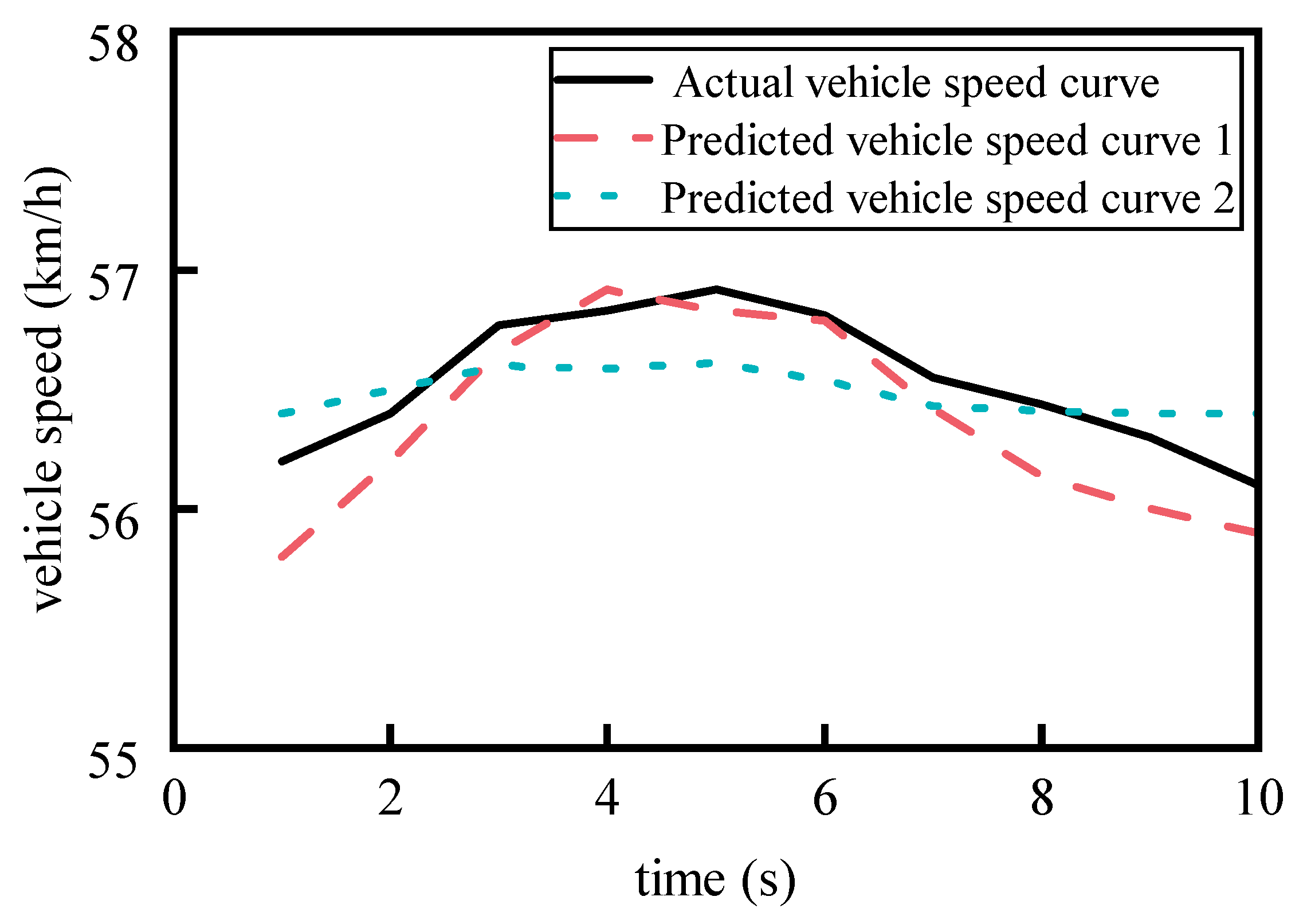
However, when vehicle speed prediction is applied to predictive control problems—particularly in hybrid vehicle energy management—different application domains impose fundamentally different requirements on prediction results. In hybrid energy management, vehicle speed represents the instantaneous energy demand state, while vehicle acceleration characterizes the variation trend of energy demand. Both factors play a critical role in power split decisions and energy consumption optimization. Consequently, an effective predicted speed profile should not only minimize numerical deviation from the actual speed but also accurately capture the temporal variation and trend characteristics of vehicle speed [7]. Existing evaluation indicators for vehicle speed prediction, such as RMSE and MAE, primarily quantify pointwise numerical distance between predicted and actual speed values [8]. These metrics inherently neglect the similarity of speed variation trends and dynamic patterns. As illustrated in Figure 1, two predicted speed curves with identical MAE values (0.184 km/h) exhibit markedly different shape similarities relative to the actual speed trajectory. Predicted speed curve 2 demonstrates a closer match in trend and dynamic behavior, despite having the same MAE as predicted speed curve 1. This discrepancy arises because MAE only considers instantaneous numerical differences and completely ignores the structural and temporal characteristics of speed evolution.

Figure 1. 10 s speed segment on a data set.

In predictive energy management strategies, predicted speed trajectories are mainly used to guide power source selection and power distribution in order to reduce overall energy consumption [9]. As a result, a predicted speed curve that appears optimal under distance-based evaluation metrics may lead to suboptimal energy consumption performance, or even significant deviation from the theoretical optimal energy consumption, when integrated into energy management optimization. Similar limitations also exist for other commonly used metrics such as RMSE and R². Therefore, evaluation indicators that rely solely on numerical distance without considering the application context of predictive energy management may fail to reflect the true effectiveness of vehicle speed prediction.

To address this gap between application-specific requirements and existing evaluation capabilities, it is necessary to investigate whether a stable and consistent relationship exists between energy consumption deviation—relative to theoretical optimal performance—and different speed prediction evaluation indicators. Furthermore, it is essential to explore evaluation metrics that are more aligned with the objectives of energy consumption optimization. Accordingly, this study focuses on the effectiveness evaluation of vehicle speed prediction from the perspective of predictive energy management.

2. Research Method for Evaluating the Validity of Vehicle Speed Prediction Curves

2.1. Overall Framework of the Research Method

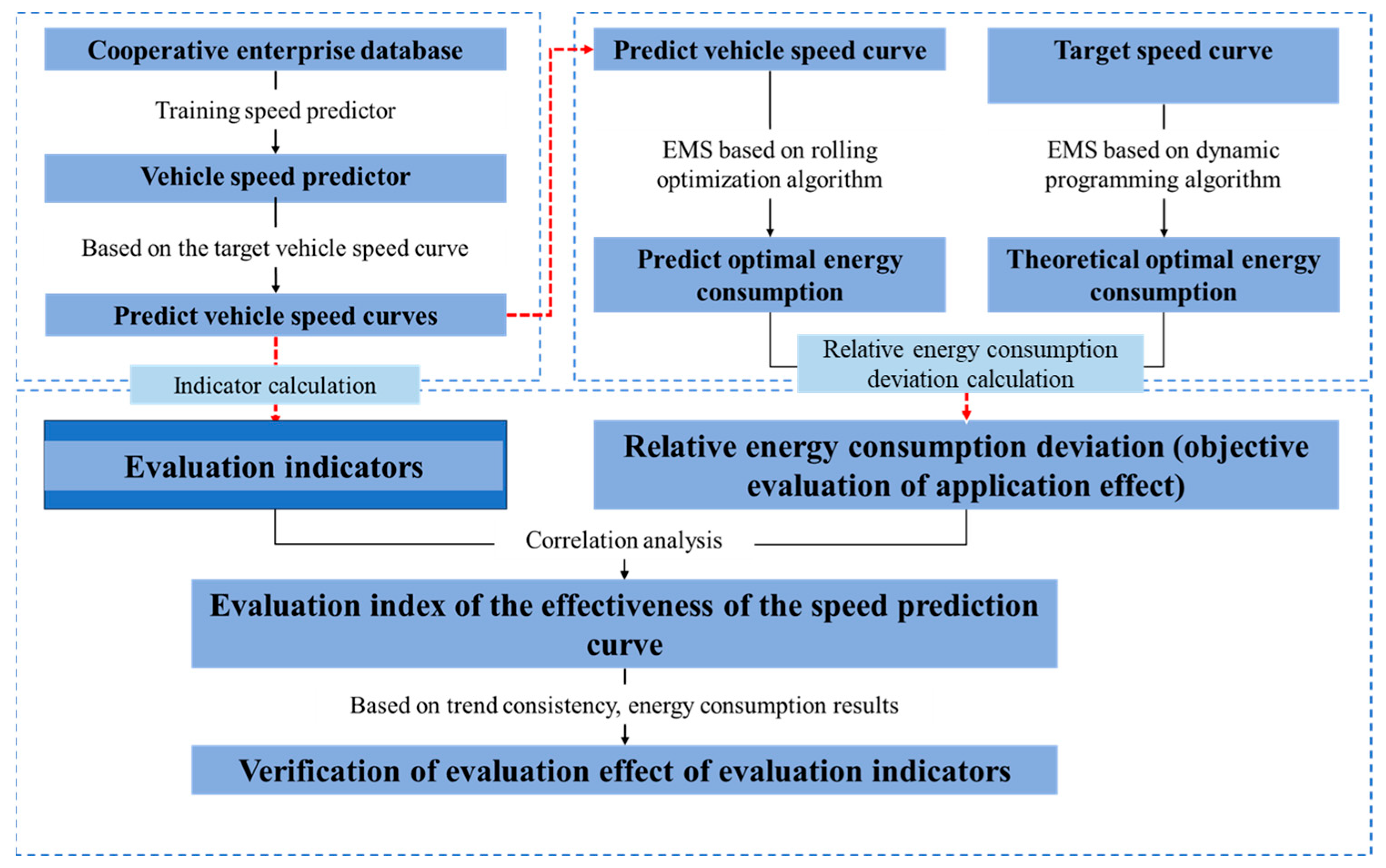
The work of evaluating the effectiveness of predicted vehicle speed curves includes four steps: (1) obtaining predicted vehicle speed curves from different vehicle speed predictors to form basic data; (2) establishing an objective evaluation method for the application effect of predicted vehicle speed curves; (3) evaluating the effectiveness of the evaluation indicators used in the development of the current predicted speed curves based on the correlation analysis results between the application effect of the predicted speed curves and the evaluation indicators of the predicted curves; (4) exploring more effective evaluation indicators for use in the research of predictive energy management strategies.

The logical framework of the research work is shown in Figure 2, and the specific content of each work step is described as follows.

Figure 2. Research content framework diagram.

Obtaining predicted speed curves with different prediction levels is the basis of this study. To construct a relatively fair comparison basis, the development of vehicle speed prediction models was carried out based on a passenger car driving database provided by a cooperative enterprise. This database includes information such as vehicle speed, acceleration, and pedal opening. A variety of constructed vehicle speed predictors were trained using this information, and the introduction of each vehicle speed predictor is provided in Section 2.2.1.

To avoid the impact of differences in the capabilities of energy management strategies themselves on the effect of energy consumption optimization during the process of optimizing powertrain energy distribution, in this study, dynamic programming algorithm and rolling optimization algorithm were used for energy management of the powertrain based on the actual speed curve and the predicted speed curve, respectively. The specific descriptions of these two optimization algorithms are given in Section 2.3.2. These two optimization algorithms can calculate the theoretical optimal energy consumption when energy management is performed using the actual speed curve and the execution energy consumption when energy management is performed using the predicted speed curve, respectively. Then, the relative energy consumption deviation is calculated based on the deviation between the theoretical optimal energy consumption and the execution energy consumption. The relative energy consumption deviation is used to characterize the effectiveness of the predicted speed curve, thereby reducing the impact of the energy management strategy during the research process. The definition of the relative energy consumption deviation is provided in Section 2.3.3.

Correlation analysis was conducted between the values of different evaluation indicators corresponding to the predicted speed curves and the relative energy consumption deviation to evaluate the effectiveness of the currently used evaluation indicators for predicted speed curves. On this basis, further exploration was made into highly effective evaluation indicators for predicted speed curves for use in the research of predictive energy management strategies.

2.2. Preparation of Predicted Vehicle Speed Curves

To obtain predicted vehicle speed curves, data was collected from a certain commuting route for 7 days, with a daily driving distance of 52 ± 1 km. These routes were randomly selected as target speed curves, and corresponding predicted speed curves were obtained through trained Long Short-Term Memory (LSTM) [10], Gated Recurrent Unit (GRU) [11], and Temporal Convolutional Network (TCN) [12] speed predictors, respectively.

2.2.1. Acquisition of Predicted Vehicle Speed Curves

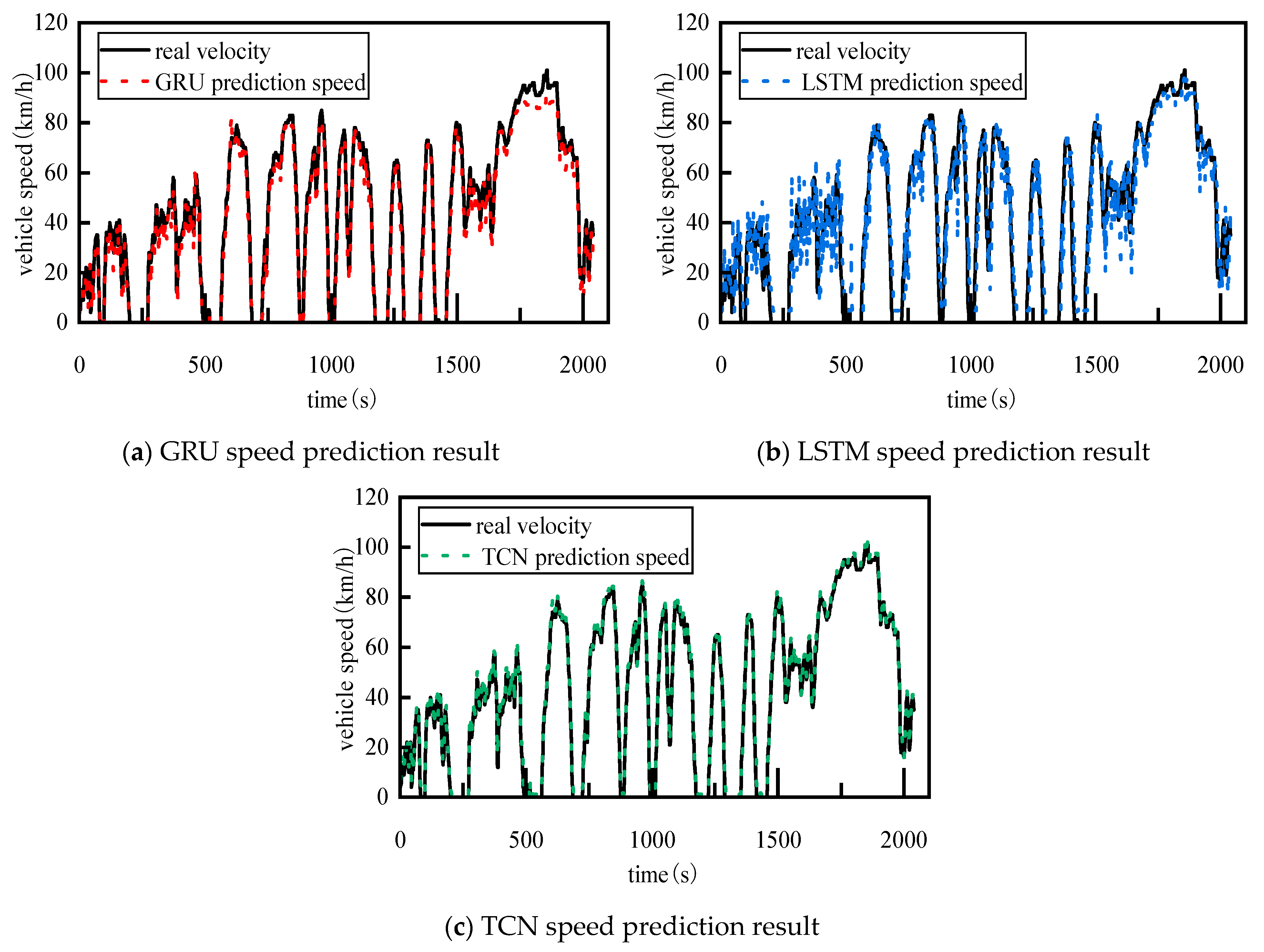
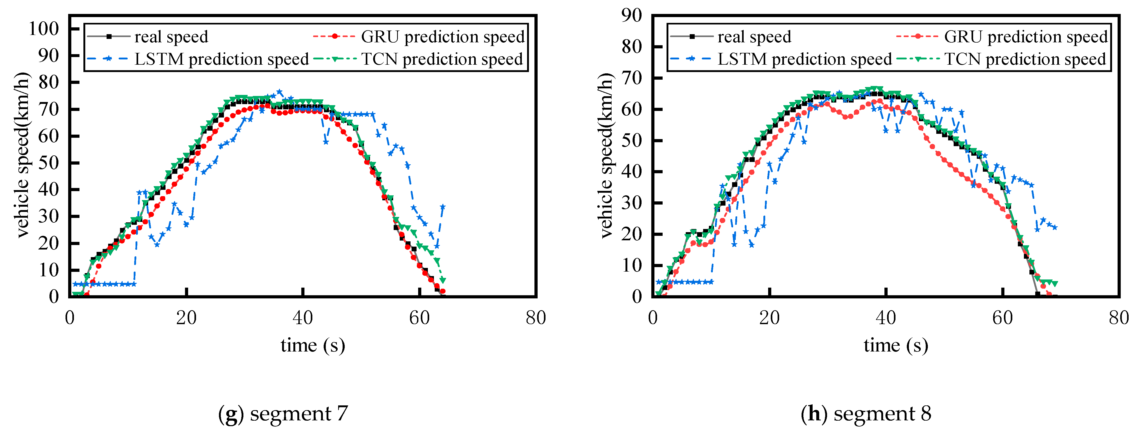
Since the focus of this study is on obtaining evaluation indicators for predicted speed curves, the above-mentioned speed predictors adopted classical architectures in their development and were trained using a database containing 35,840 s of real vehicle data provided by the cooperative enterprise. Using the trained speed predictors and the target speed curves collected from the real vehicles mentioned above, the speed prediction results of different speed predictors were obtained as shown in Figure 3.

Figure 3. Speed prediction results.

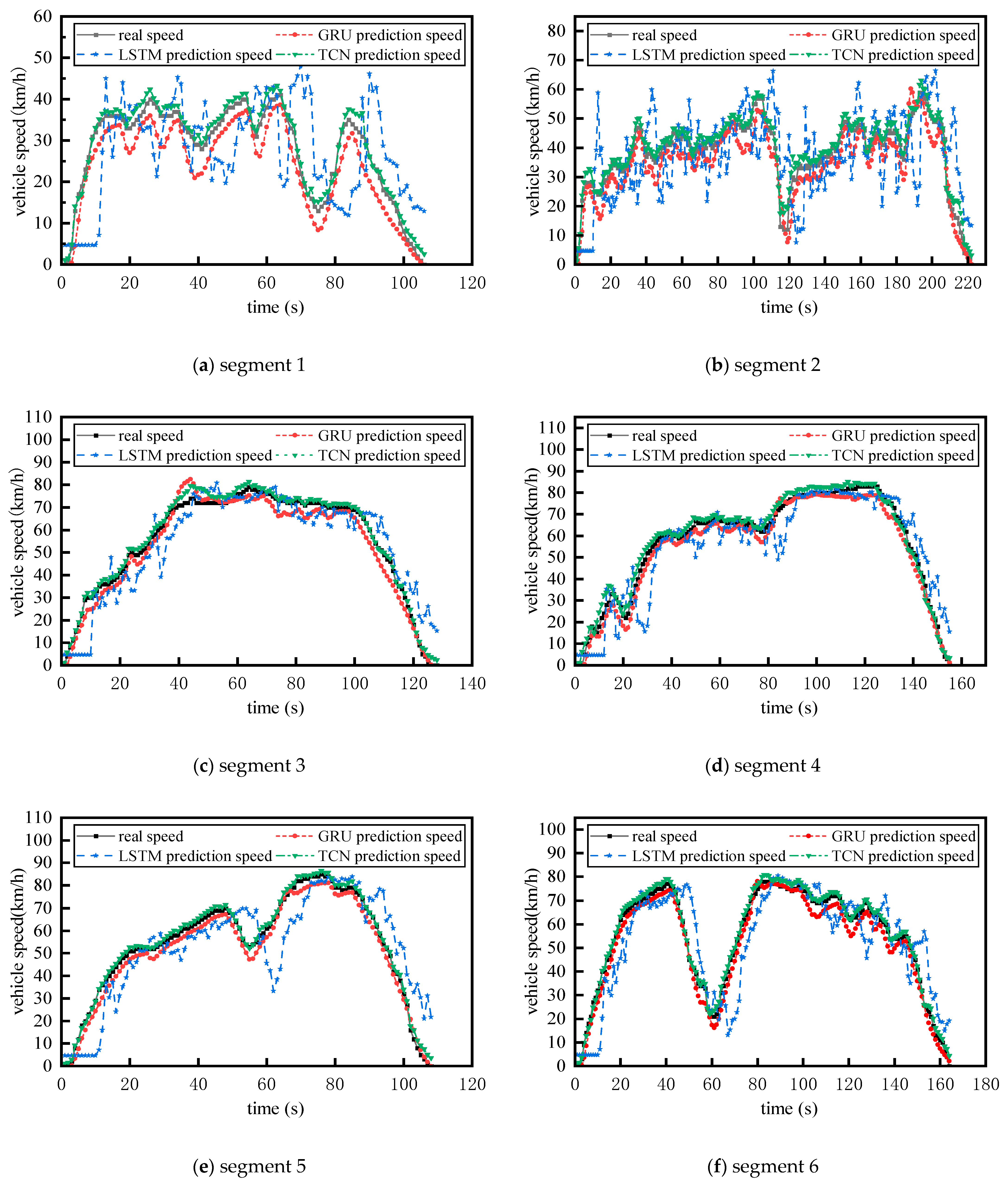
To cover all characteristics of the object during motion and enhance applicability, the real speed curves and predicted speed curves were divided into 8 complete kinematic segments according to the complete process of stationary-acceleration-driving-deceleration-parking in the study, as shown in Figure 4.

Figure 4. The segmentation results of vehicle speed segments covering all features of the motion process.

2.2.2. Analysis of Vehicle Speed Prediction Results

Two commonly used statistical indicators, MAE and RMSE, were selected for analyzing the vehicle speed prediction results [13]. It is generally believed that smaller values of MAE and RMSE indicate better vehicle speed prediction results [14]. The specific calculation formulas for RMSE and MAE are shown in Equations (1) and (2).

$$MAE={\displaystyle \frac{1}{n}}\sum _{i=1}^n|\left({\widehat{y}}_i-y_i\right)|$$

(1)

$$RMSE=\sqrt{{\displaystyle \frac{1}{n}}\sum _{i=1}^n{({\widehat{y}}_i-y_i)}^2}$$

(2)

In the above equations, ${\widehat{y}}_i$ is the predicted vehicle speed at time $i$ within the prediction period, $y_i$ is the actual vehicle speed at time $i$ within the prediction period, ${\overline{y}}_i$ is the average of the actual vehicle speeds within the prediction period, and $n$ is the number of vehicle speed data points within the prediction period.

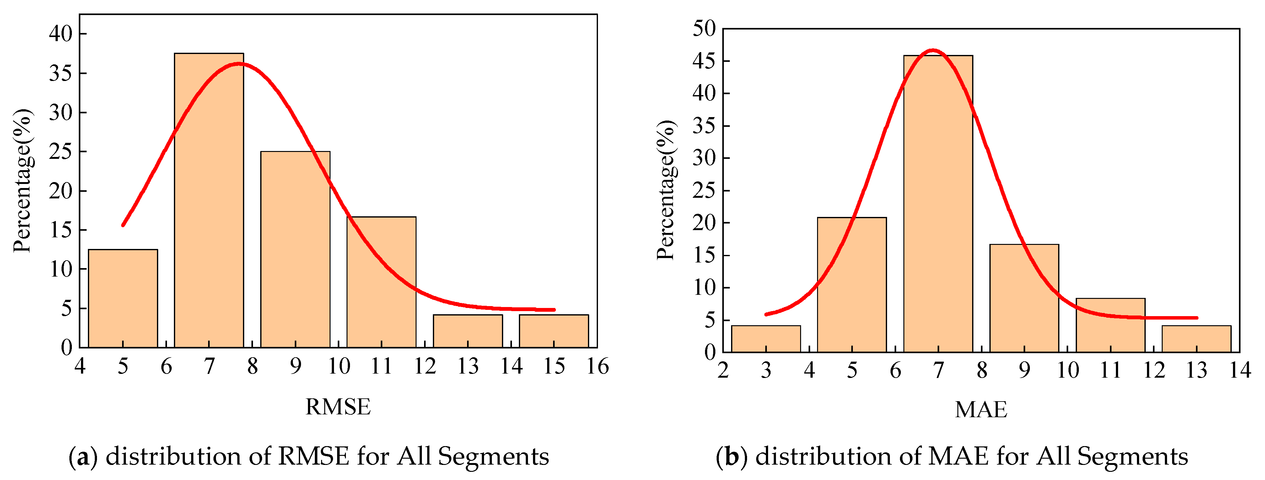
The RMSE and MAE results between the predicted speed and the actual speed in each prediction domain at all times within each segment were averaged, and finally, the distribution results of the average RMSE and MAE of different predicted speed curves for each segment are shown in Figure 5.

Figure 5. Distribution results of RMSE and MAE for all segments.

From the RMSE and MAE distribution results of all segments presented in Figure 5, it can be observed that the aforementioned vehicle speed predictor exhibits a small prediction deviation in most scenarios. Its error levels are concentrated, and the proportion of extreme deviations is low, which demonstrates that the predictor possesses high basic prediction accuracy.

2.3. Acquisition of Energy Consumption Deviation Data

By applying the obtained predicted speed curves and actual speed curves to the predictive energy management strategy of hybrid systems, the execution energy consumption based on the predicted speed curves and the theoretically achievable optimal energy consumption based on the actual speed curves can be obtained. The degree of deviation between the two, namely the relative energy consumption deviation, is used as the basis for judging the effectiveness of the predicted speed curves in practical applications.

2.3.1. Hybrid Vehicle Simulation Platform and Predictive Energy Management Strategy

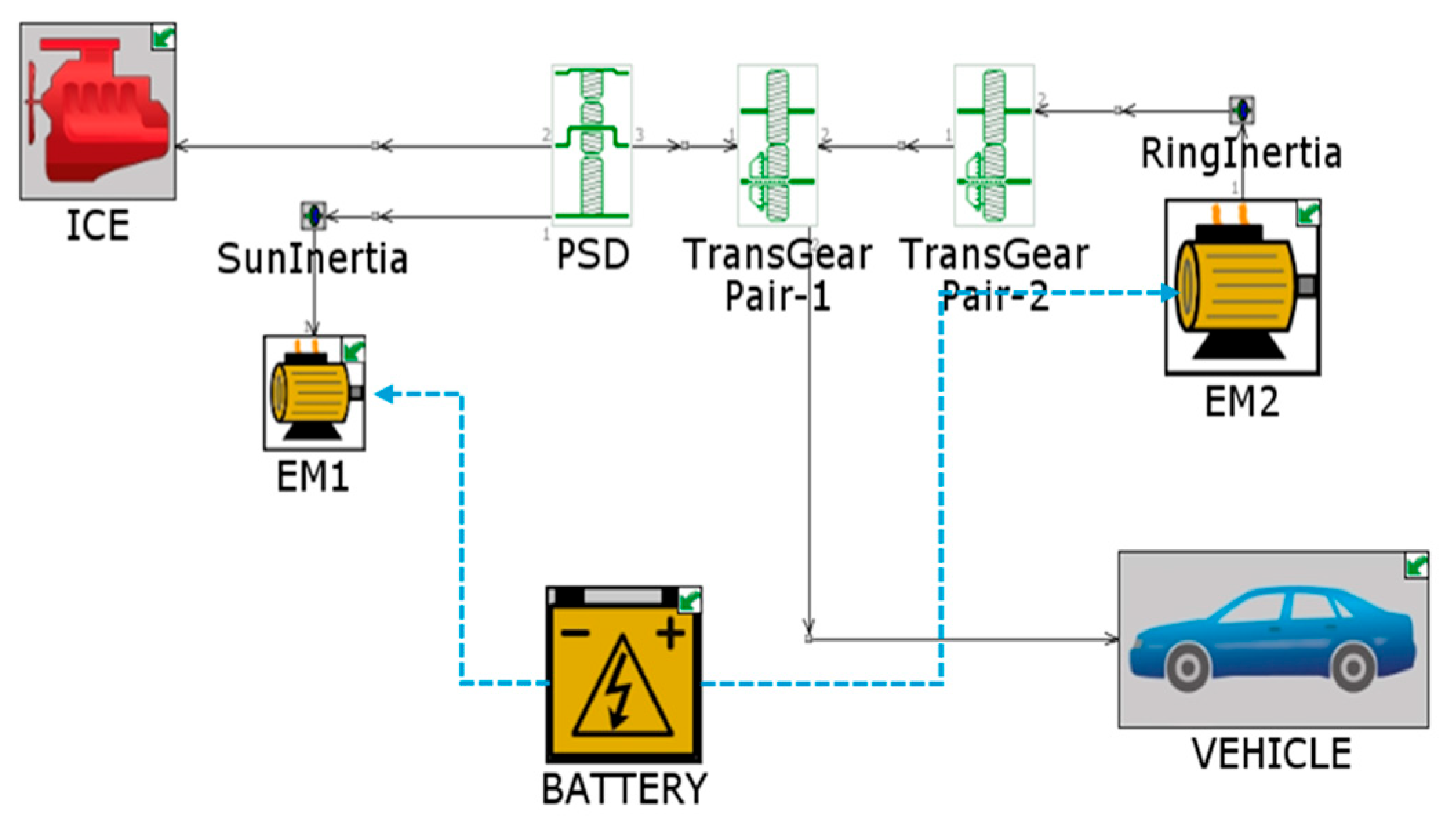
The existing, verified and highly accurate PHEV model in the previous research is taken as the object model for the energy management strategy based on MPC, as shown in Figure 6 [15]. The structure of this model is as follows: MPC can generate reference information within a short time domain by establishing a predictive model of the controlled object, and constrain the value ranges of input and output variables within the feasible domain. Eventually, the global optimization problem is transformed into a local optimal problem.

Figure 6. PHEV model based on GT-SUITE.

2.3.2. Acquisition of Theoretical Optimal Energy Consumption and Execution Energy Consumption

Dynamic programming [16] (DP) algorithm is a numerical optimization method that seeks the global optimal solution through backward-time operation. It is widely applied in various predictive energy management strategies for transportation vehicles [17]. The DP algorithm gradually solves the local optimal solution for each stage and stores the intermediate results. Eventually, by gradually accumulating energy consumption and comparing the results of different paths, the global optimal energy consumption plan from the starting point to the destination is found. This process ensures that the energy consumption results obtained through the DP algorithm for the entire process of real vehicle speed offline global energy management are optimal, that is, the optimal energy consumption results that can be theoretically achieved.

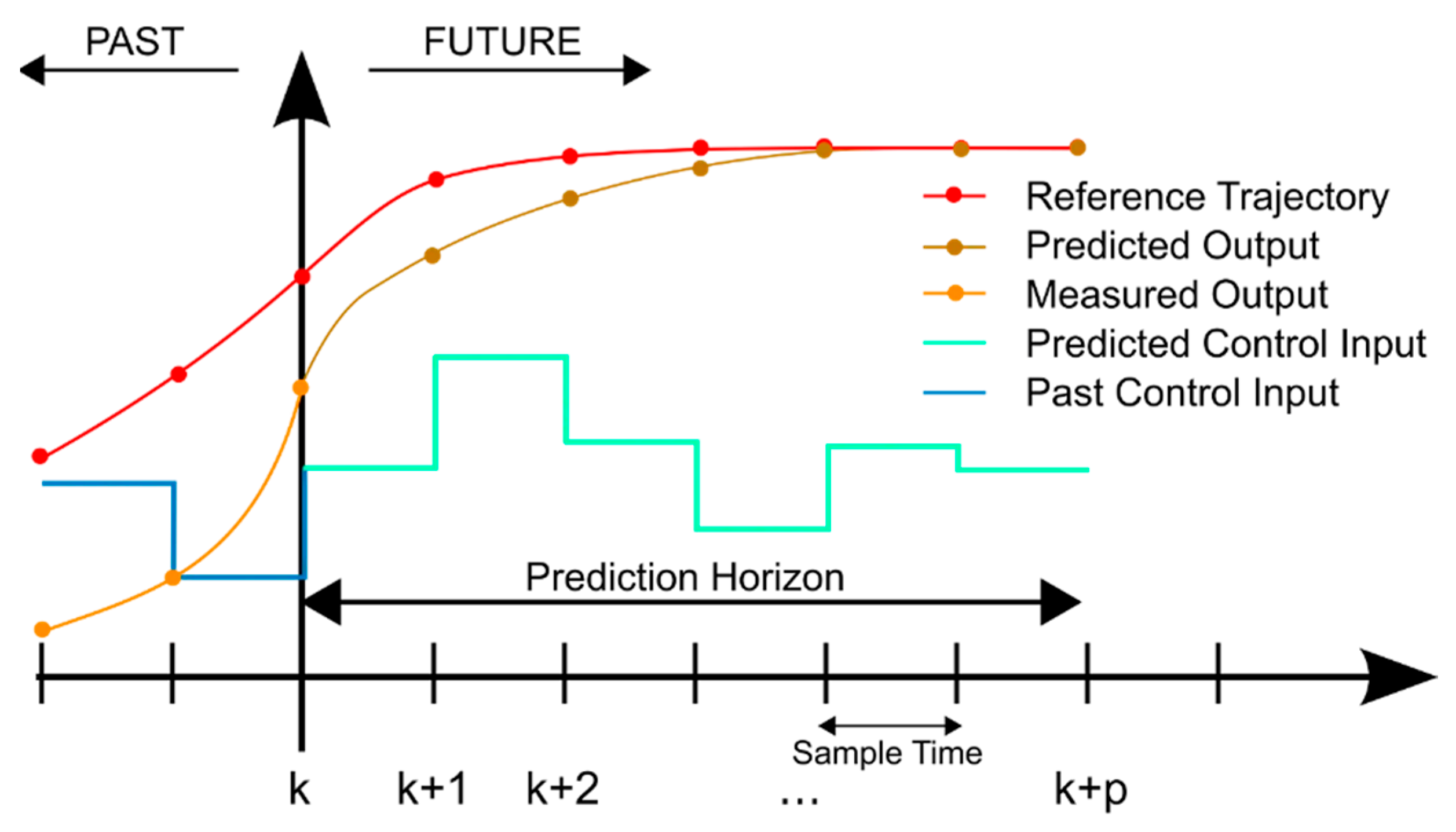
When applying the predicted vehicle speed results to perform energy management calculations and execute energy consumption, since global vehicle speed information cannot be obtained, it is necessary to convert the global optimization problem into a local optimal problem and perform local optimal energy management for the system [18]. The specific process is shown in Figure 7.

Figure 7. Rolling optimization process.

Among them, $k+1-k+p$ respectively represent the control time domain and the prediction time domain; $r$ is the reference trajectory; $e_k$ is the deviation term between the output and the reference trajectory. At each time domain of vehicle speed prediction, the control sequence that minimizes the energy consumption function is solved, and the first value of this control sequence is applied to the system to obtain the actual output of the system. This output is then used as feedback to correct the deviation of the prediction model and achieve local energy management for the vehicle within the prediction time domain. The prediction and control are repeatedly carried out at each time step to form a rolling optimization process.

During the time domain of vehicle speed prediction, solve the control sequence that minimizes the energy consumption function, and apply the first value of this control sequence to the system to obtain the actual output of the system. Then, use this as feedback to correct the deviation of the prediction model and achieve local energy management for the vehicle within the prediction time domain. The prediction and control are repeatedly carried out at each time step to form a rolling optimization process.

Based on the real vehicle speed curve of each segment and using the DP algorithm, perform global energy management for the hybrid power system, obtaining the theoretical optimal energy consumption corresponding to each real vehicle speed curve segment; using the rolling optimization method, perform local optimal energy management for the power system based on the predicted vehicle speed curve, obtaining the execution energy consumption corresponding to each predicted vehicle speed curve segment. Finally, the energy consumption results for each segment are as shown in Table 1.

Table 1. Energy consumption results for each segment.

Energy Consumption	Theoretical Optimal Energy Consumption (g)	The Execution Energy Consumption of The GRU Predictor (g)	The Execution Energy Consumption of The LSTM Predictor (g)	The Execution Energy Consumption of The TCN Predictor (g)
Segment 1	10.41	26.16	28.80	34.46
Segment 2	31.84	78.80	90.64	82.13
Segment 3	34.67	45.17	65.91	46.31
Segment 4	51.19	72.38	92.45	64.08
Segment 5	37.79	48.41	62.34	49.14
Segment 6	42.75	74.50	49.37	44.40
Segment 7	17.21	19.01	30.26	23.51
Segment 8	26.05	28.73	35.78	29.53

2.3.3. Relative Energy Consumption Deviation

In the real-time energy management of the powertrain using predicted vehicle speeds, since global speed information cannot be obtained, the execution energy consumption of local optimal energy management of the powertrain based on predicted speeds cannot reach the theoretically optimal energy consumption and will be greater than the theoretical optimal energy consumption. As shown in Table 1, the execution energy consumption of the predictors for segments 1 and 2 even exceeds 200% of the theoretical optimal energy consumption. Based on the characteristic that the execution energy consumption is higher than the theoretical optimal energy consumption, when objectively evaluating the effectiveness of the vehicle speed prediction results, the theoretical optimal energy consumption can be selected as the energy consumption benchmark. When energy management is performed based on predicted speeds, the closer the execution energy consumption is to the theoretical optimal energy consumption, the better the execution energy consumption result, and it also indicates that the application of the vehicle speed prediction result to the energy management of the powertrain is more effective. To quantify the effectiveness of vehicle speed prediction, the indicator of relative energy consumption deviation was selected. The relative energy consumption deviation is the deviation between the execution energy consumption and the theoretical optimal energy consumption, and its specific calculation method is shown in Equation (3).

$$x_{eng}={\displaystyle \frac{E_{pre}-E_{real}}{E_{real}}}$$

(3)

In the above equation, $x_{eng}$ is the relative energy consumption deviation between the theoretical optimal energy consumption and the execution energy consumption, $E_{real}$ is the theoretical optimal energy consumption corresponding to the actual speed in each prediction period, and $E_{pre}$ is the execution energy consumption corresponding to the predicted speed in each prediction period. According to the definition of relative energy consumption deviation in Equation (3), the closer $x_{eng}$ is to 0, the closer the execution energy consumption is to the theoretical optimal energy consumption, and the higher the effectiveness of applying the vehicle speed prediction result to the energy management of the powertrain.

The relative energy consumption deviation results for each segment are shown in Table 2. The closer the relative energy consumption deviation result is to 0, the better the effectiveness of the vehicle speed prediction method in that segment.

Table 2. The relative energy consumption of the predicted speed and the real speed for each segment.

Relative Energy Consumption	Energy Consumption Deviation of GRU Predictor	Energy Consumption Deviation of LSTM Predictor	Energy Consumption Deviation of TCN Predictor
Segment 1	1.51	2.06	1.50
Segment 2	1.47	1.85	1.58
Segment 3	0.30	0.90	0.34
Segment 4	0.41	0.81	0.25
Segment 5	0.28	0.65	0.30
Segment 6	0.74	0.15	0.04
Segment 7	0.10	0.76	0.37
Segment 8	0.10	0.37	0.13

3. Analysis of Effectiveness Evaluation of Vehicle Speed Prediction Results

3.1. Correlation Analysis of Vehicle Speed Prediction Result Evaluation Indicators

After obtaining the relative energy consumption deviation results, correlation analysis was conducted between the evaluation indicators and the relative energy consumption deviation. By comparing the correlation between the evaluation indicators and the relative energy consumption deviation, it was determined which indicator has a stronger correlation with the relative energy consumption deviation and is more suitable as an evaluation indicator for the effectiveness of vehicle speed prediction.

3.1.1. Pearson Correlation Coefficient

To determine the strength of the correlation between the evaluation indicators and the relative energy consumption deviation, the Pearson correlation coefficient [19] was selected as the basis for judging the strength of the correlation. The Pearson correlation coefficient is a statistical measure used to quantify the linear correlation between two variables [20], and its specific calculation method is shown in Equation (4).

$$r={\displaystyle \frac{\sum \left(X-\overline{X}\right)\left(Y-\overline{Y}\right)}{\sqrt{\sum (X-\overline{X}{)}^2}\sqrt{\sum (Y-\overline{Y}{)}^2}}}$$

(4)

where $r$ represents the Pearson coefficient, and its value ranges from −1 to 1. The sign of $r$ indicates whether the two variables are positively or negatively correlated, and the magnitude of r represents the strength of the correlation. The closer the absolute value is to 1, the stronger the correlation between the two variables; the closer to 0, the weaker the correlation. $X$ and $Y$ are the values of the two variables, respectively, and $\overline{X}$, $\overline{Y}$ are the means of $X$ and $Y$, respectively.

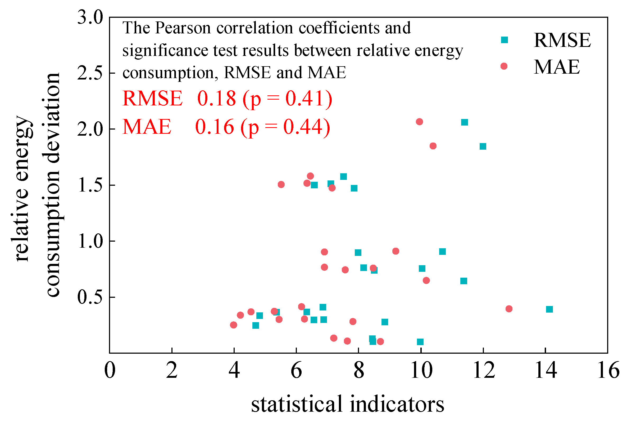
Based on the results of the root mean square error (RMSE), mean absolute error (MAE), and relative energy consumption deviation between the predicted speeds and the actual speeds obtained by the three speed predictors in Section 2.2.1, we conducted a correlation analysis using the Pearson correlation coefficient and performed a significance test on the results of the correlation analysis. The distribution and correlation results of relative energy consumption deviation, RMSE, and MAE are shown in Figure 8.

Figure 8. Correlation between statistical indicators (RMSE and MAE) and relative energy consumption deviation.

From Figure 8, it can be observed that the relationships between the traditional statistical indicators RMSE, MAE and the relative energy consumption deviation present a relatively scattered distribution pattern. Their Pearson correlation coefficients are 0.18 and 0.16 respectively. This indicates that the correlations between these indicators and the relative energy consumption deviation are weak. Additionally, the results of the significance analysis show that the correlation between relative energy consumption and RMSE did not pass the statistical significance test (p = 0.41), and the correlation between relative energy consumption and MAE was also not significant (p = 0.43). These results further indicate that the traditional RMSE and MAE indicators are difficult to effectively reflect the impact of the prediction speed curve on the energy consumption results in a statistical sense. Their ability to evaluate the effectiveness of the prediction speed curve in energy management strategy application scenarios for assessing the validity is significantly limited.

3.1.2. Correlation Analysis of Other Indicators

To further explore indicators that can effectively evaluate the vehicle speed prediction results, the correlation between similarity indicators and vehicle speed characteristic indicators and the relative energy consumption deviation was further analyzed.

Similarity indicators refer to metrics used to measure the degree of similarity between two or more datasets when comparing them. In this study, three commonly used distance indicators, namely Euclidean distance, Manhattan distance, and Chebyshev distance, were selected for vehicle speed similarity indicators. Smaller values of these three distance indicators indicate that the predicted curve is more similar to the actual curve. The specific calculation formulas for Euclidean distance, Manhattan distance, and Chebyshev distance are shown in Equations (5)–(7).

$$d_{eud}=\sqrt{\sum _{i=1}^n{(x_i-y_i)}^2}$$

(5)

$$d_{mand}=\sum _{i=1}^n|x_i-y_i|$$

(6)

$$d_{chebd}=\underset{k\to \infty }{lim} {\left(|(x_i-y_i){|}^{{\displaystyle \frac{1}{k}}}\right)}^k$$

(7)

In the above equations, $d_{eud}$, $d_{mand}$ and $d_{chebd}$ are Euclidean distance, Manhattan distance, and Chebyshev distance, respectively. $x_i$ is the predicted vehicle speed at time $i$ within the prediction period, $y_i$ is the actual vehicle speed at time $i$ within the prediction period, and $n$ is the number of vehicle speed data points within the prediction period.

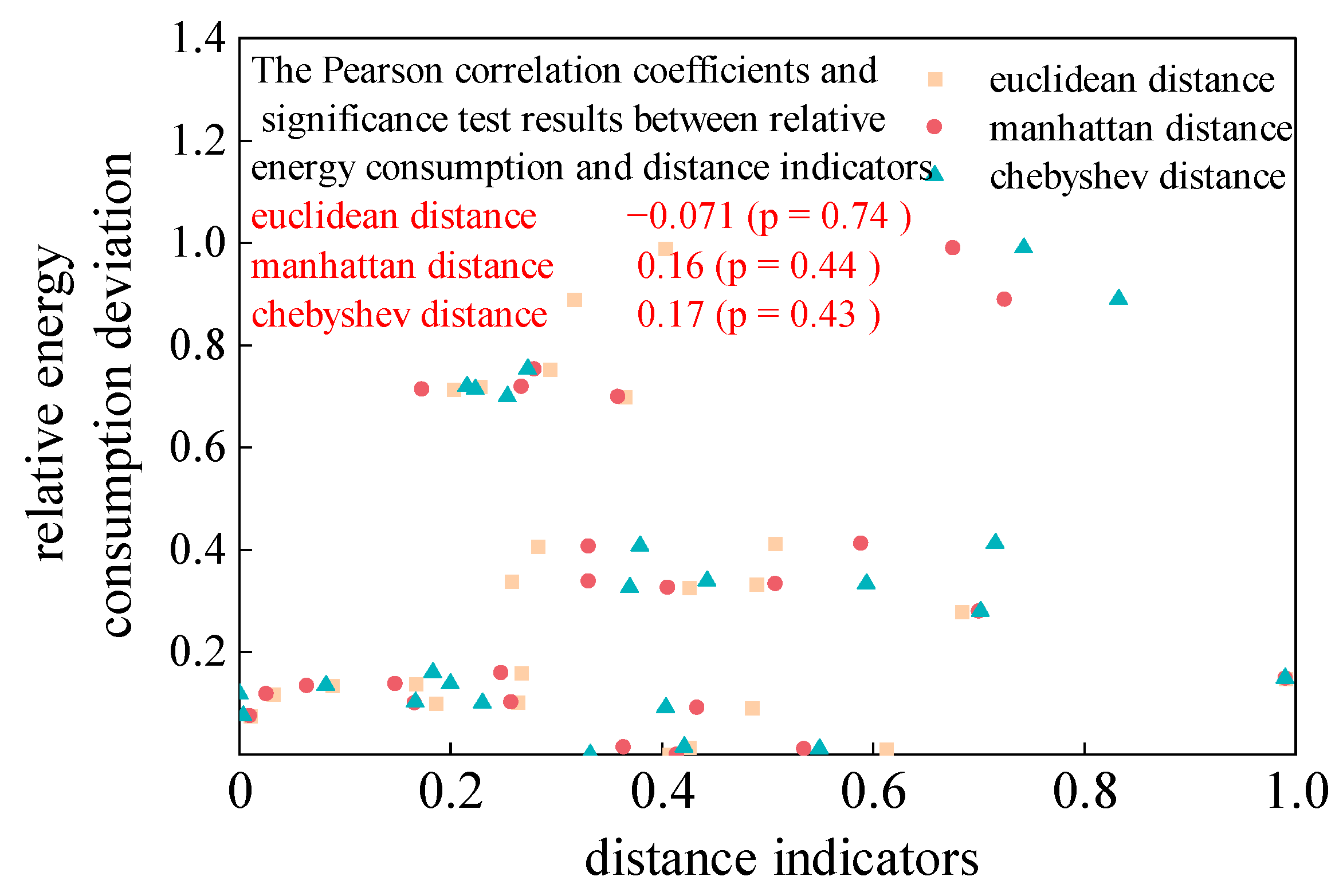
Based on the 8 motion segments determined in Section 2.2.1, the results of the Euclidean distance, Manhattan distance, and Chebyshev distance between the predicted speed and the actual speed within each time prediction interval for the 24 predicted speed curves obtained under the three speed predictors were averaged. Then, the correlation between the average indicators and the relative energy consumption was analyzed. Finally, Figure 9 shows the standardized distribution of the relative energy consumption deviation and distance indicators for each segment, as well as the results of their correlation and significance tests.

Figure 9. Correlation between distance-based indicators and relative energy consumption deviation.

In terms of vehicle speed characteristics, the average speed, maximum speed, acceleration time proportion, and deceleration time proportion were selected as the indicators for correlation analysis with the relative energy consumption deviation. Their calculation methods are as shown in Equations (8)–(11).

$$v_{avg}={\displaystyle \frac{{\sum }_{i=1}^n v_i·\Delta t}{T_{total}}}$$

(8)

$$v_{max}=max\left\{v_1,v_2,\dots ,v_n\right\}$$

(9)

$${\eta }_{\mathrm{a}\mathrm{c}\mathrm{c}}={\displaystyle \frac{T_{\mathrm{a}\mathrm{c}\mathrm{c}}}{T_{\mathrm{total}}}}\times 100\%$$

(10)

$${\eta }_{\mathrm{dec}}={\displaystyle \frac{T_{\mathrm{dec}}}{T_{\mathrm{total}}}}\times 100\%$$

(11)

The calculation of the average speed of each segment is as shown in Equation (8), where $v_{\mathrm{avg}}$ is the average speed, $v_i$ represents the instantaneous speed at the i-th sampling time, $\Delta t$ is the length of the sampling time interval, $n$ is the total number of samples in each segment, and $T_{total}$ is the total time of each segment. The calculation method for the maximum speed of each segment is as shown in Equation (9), where $v_{max}$ represents the maximum speed of each segment. The calculation methods for the proportion of acceleration time and deceleration time for each segment are as shown in Equations (10) and (11). Here, ${\eta }_{\mathrm{a}\mathrm{c}\mathrm{c}}$ and ${\eta }_{\mathrm{dec}}$ represent the proportion of acceleration time and deceleration time, respectively, which are calculated by dividing the acceleration time $T_{\mathrm{a}\mathrm{c}\mathrm{c}}$ and deceleration time $T_{\mathrm{dec}}$ by the total time of each segment. The sampling moments where the instantaneous acceleration $a_i$ is greater than 0.15 $\mathrm{m}·{\mathrm{s}}^{-2}$ are defined as acceleration moments, while the sampling moments where the instantaneous acceleration $a_i$ is less than −0.15 $\mathrm{m}·{\mathrm{s}}^{-2}$ are defined as deceleration moments. The acceleration is calculated through the forward difference method.

Among the vehicle speed characteristics, average speed and maximum speed can reflect to a certain extent whether the vehicle is driving at a low or high speed on the road over a period of time; while acceleration time proportion and deceleration time reflect whether the vehicle is in an accelerating, decelerating, or idling state overall over a period of time. To eliminate the impact of data magnitude and more intuitively measure the relative impact of vehicle speed characteristic deviations, after calculating the above indicators for predicted and actual speeds, the relative deviation between them was further calculated, and the specific calculation method is shown in Equation (12).

$$E_r=|{\displaystyle \frac{x_r-x_{pre}}{x_r}}|$$

(12)

In the above equation, $E_r$ is the relative deviation between the predicted speed indicator and the actual speed indicator in the prediction period, $x_r$ is the actual speed indicator in each prediction period, and $x_{pre}$ is the predicted speed indicator in each prediction period.

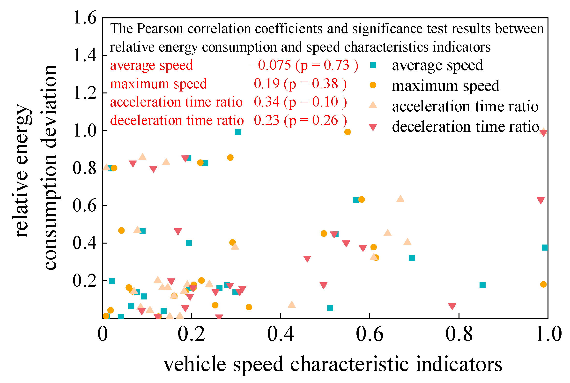
The average relative deviation of vehicle speed characteristics indicators between predicted speed and actual speed at all times on 24 speed curves of 8 sections was calculated. The correlation between the average indicator results and relative energy consumption was analyzed. Finally, Figure 10 shows the standardized distribution of relative energy consumption deviation and speed characteristic indicators for each section, as well as the results of their correlation and significance test.

Figure 10. Correlation between vehicle speed characteristic indicators and relative energy consumption deviation.

By comparing the correlation results and significance test results of each evaluation index with the relative energy consumption deviation in Figure 8, Figure 9 and Figure 10, it was found that among the calculated indicators, except for the deviation of the acceleration time proportion, the correlations of other indicators with relative energy consumption were weak. The Pearson correlation coefficient was lower than 0.3, and the p-values of the significance test results were all far greater than 0.05, indicating that these indicators were difficult to effectively reflect the energy consumption change characteristics. In contrast, the acceleration time ratio deviation indicator showed a higher correlation with relative energy consumption. Its Pearson correlation coefficient reached 0.34, and the p-value was 0.10. Although it has not reached the traditional 0.05 significance level, it has already shown a certain correlation trend. Therefore, for each of the 24 vehicle speed curves, based on the deviation of the acceleration time ratio between the predicted and actual vehicle speeds over 8 time periods, the standard deviation was calculated. The calculation method is as shown in Formula (13).

$$\sigma =\sqrt{{\displaystyle \frac{1}{n}}\sum _{i=1}^n {(E_{{\eta }_{\mathrm{a}\mathrm{c}\mathrm{c}},i}-\mu )}^2}$$

(13)

In the above formula, $E_{{\eta }_{\mathrm{a}\mathrm{c}\mathrm{c}},i}$ represents the deviation of the acceleration time proportion at time $i$ in each segment, $\mu$ is the average value of the deceleration time proportion deviation in each segment, and $n$ is the total number of samples in each segment.

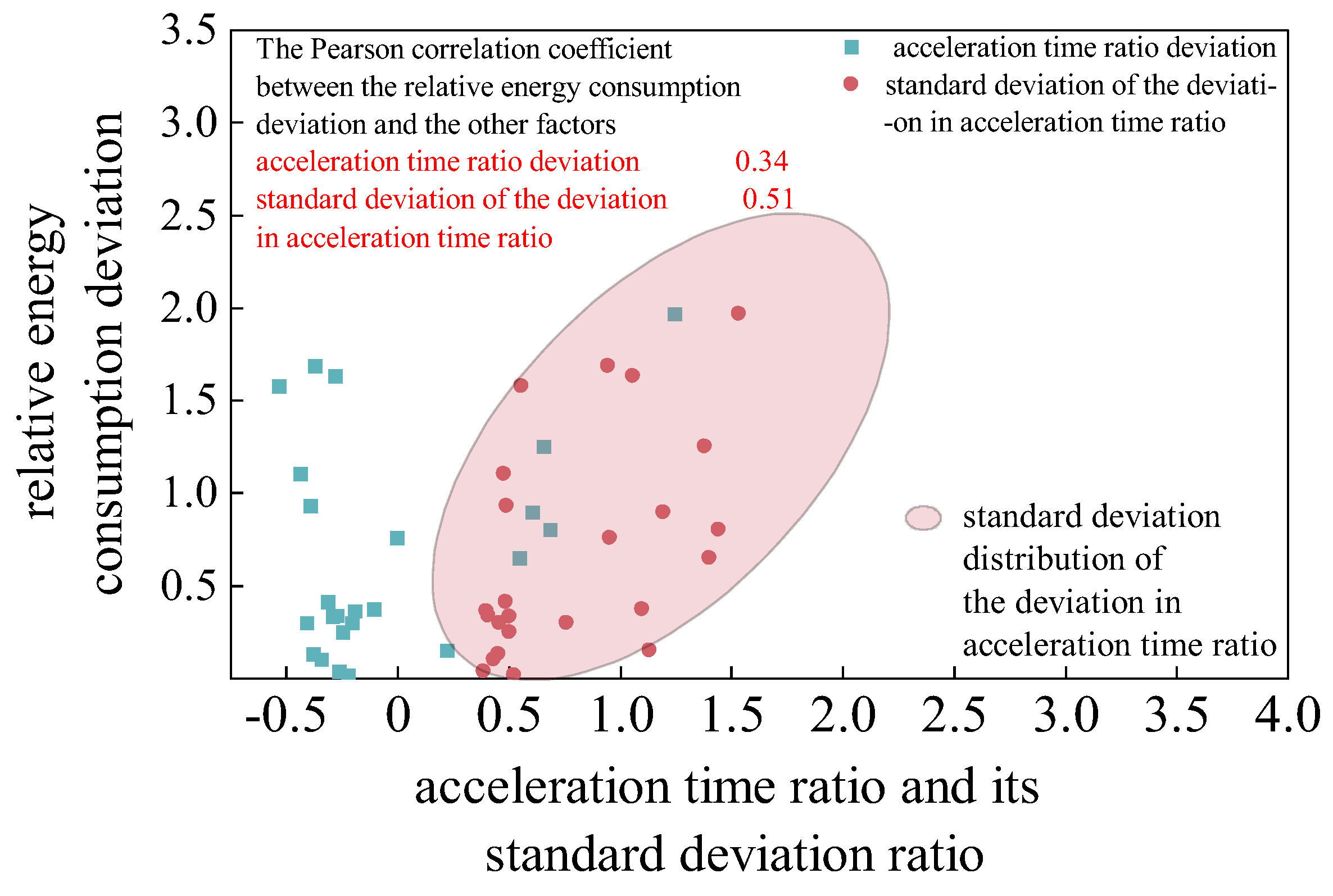
This replaced the previous method of calculating the average. Then, a correlation analysis was conducted between the results and the relative energy consumption deviation. The distribution of the results and the correlation results are shown in Figure 11.

Figure 11. Distribution and correlation of acceleration time proportion deviation metrics with relative energy consumption deviation.

As shown in Figure 11, the Pearson correlation coefficient between the deviation of acceleration time proportion and the relative energy consumption deviation is 0.34, indicating only a weak linear relationship. This result suggests that the instantaneous deviation of acceleration time proportion provides limited explanatory capability with respect to energy consumption deviation when predicted speed profiles are applied to predictive energy management strategies. By contrast, the standard deviation of the deviation in acceleration time proportion exhibits a markedly stronger correlation with relative energy consumption deviation, with a Pearson correlation coefficient of 0.51. This moderate positive correlation implies that the dispersion characteristics of acceleration behaviour deviations over the prediction horizon are more closely associated with energy consumption performance than pointwise deviation measures. Specifically, larger fluctuations in acceleration time proportion deviation tend to correspond to greater deviations in energy consumption from the theoretical optimum.

Moreover, the distribution of data points associated with the standard deviation of the acceleration time proportion deviation demonstrates a clearer and more consistent trend, as indicated by the pink elliptical region in Figure 11. The orientation and concentration of this region reveal an evident increasing tendency of relative energy consumption deviation with respect to the standard deviation of acceleration time proportion deviation. This trend consistency reflects a more stable and interpretable relationship between the proposed dispersion-based indicator and energy consumption deviation, which is not observed when using the acceleration time proportion deviation alone. The results presented in Figure 11 indicate that while the deviation of acceleration time proportion shows limited relevance to energy consumption outcomes, its standard deviation more effectively captures the dynamic inconsistency of predicted speed profiles. Consequently, the standard deviation of the acceleration time proportion deviation provides a more suitable and application-oriented indicator for evaluating the effectiveness of vehicle speed prediction in predictive energy management.

To further verify the robustness of the observed correlation results, both Pearson and Spearman correlation analyses were conducted between the standard deviation of the acceleration time proportion deviation and the relative energy consumption deviation across the 24 predicted speed curves. While the Pearson correlation coefficient evaluates linear relationships, the Spearman correlation coefficient assesses monotonic relationships, thereby providing complementary perspectives on correlation robustness. The results are shown in Table 3.

Table 3. Correlation coefficients and statistical significance between the standard deviation of acceleration time proportion deviation and relative energy consumption deviation.

Correlation Coefficient	Pearson Correlation Coefficient	Spearman Correlation Coefficient
Correlation Results	0.51	0.54
Significant Results (p-value)	0.010	0.007

Both correlation coefficients indicate a moderate positive correlation, with values of 0.51 for the Pearson correlation and 0.54 for the Spearman correlation. In addition, the associated p-values (0.010 and 0.007, respectively) demonstrate that the correlations are statistically significant at the 0.05 level. The consistency of correlation strength and statistical significance across different correlation measures confirms the stability of the relationship between the acceleration-related deviation metric and relative energy consumption deviation. These results further suggest that the standard deviation of the acceleration time proportion deviation captures essential dynamic characteristics of predicted speed profiles that are closely linked to energy consumption performance. Therefore, this indicator is well suited for evaluating the effectiveness of vehicle speed prediction in predictive energy management applications.

3.2. Validation of Vehicle Speed Prediction Effectiveness Evaluation Indicators

3.2.1. Trend Consistency Verification

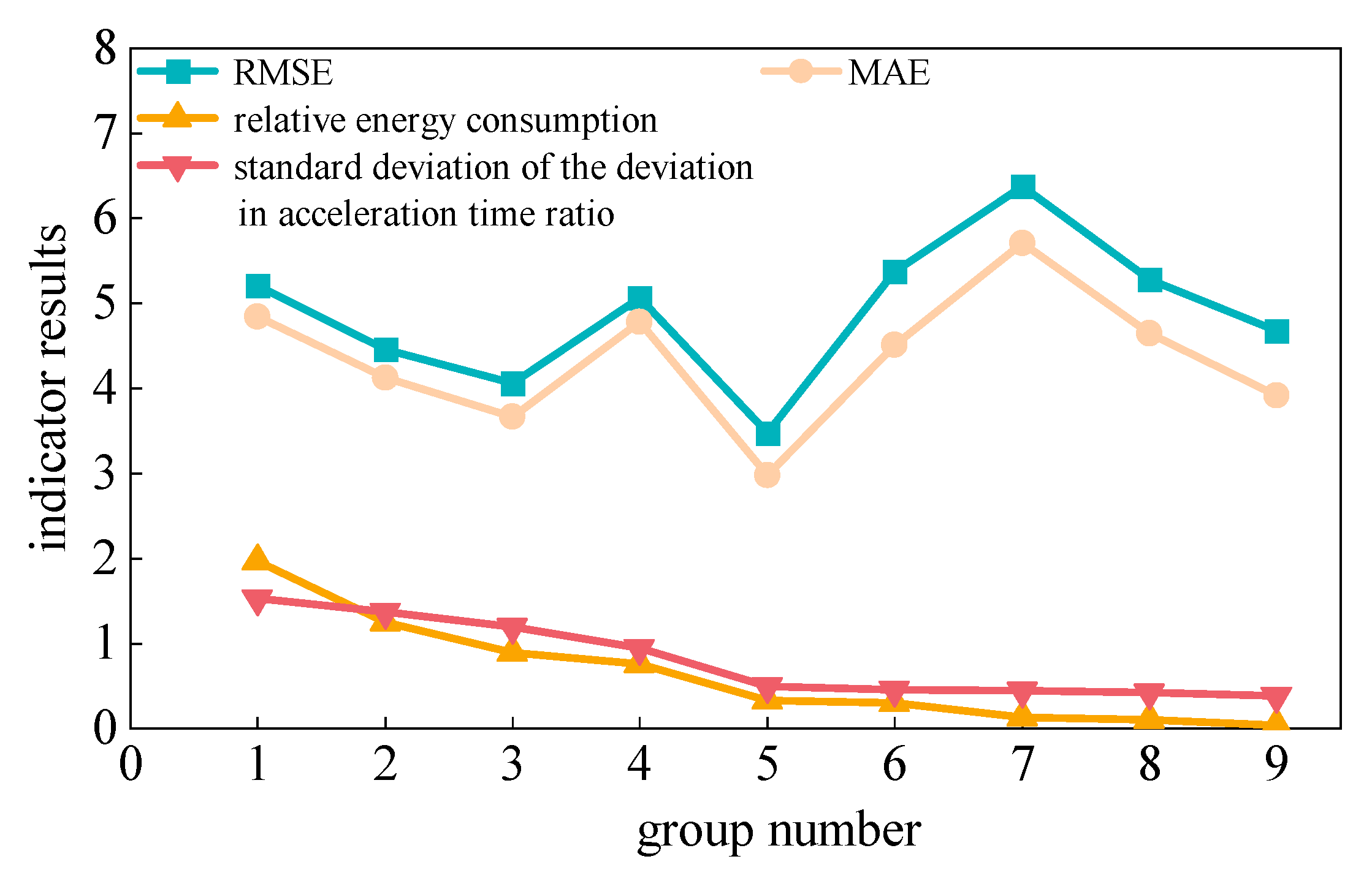
Since the correlation coefficient between the standard deviation of the deviation in acceleration time proportion and the relative energy consumption deviation is 0.51, indicating only a moderate correlation between them, to further verify that the standard deviation of the deviation in acceleration time proportion can evaluate the effectiveness of vehicle speed prediction to a certain extent, data on the standard deviation of the deviation in acceleration time proportion, RMSE, MAE, and relative energy consumption deviation were randomly selected, as shown in Figure 12.

Figure 12. Trend comparison of RMSE, MAE, and the standard deviation of acceleration time proportion deviation with relative energy consumption deviation.

It can be seen from the above figure that in the randomly selected data, as the standard deviation of the deviation in acceleration time proportion decreases, the relative energy consumption deviation approaches 0. In contrast, there is no monotonic relationship between RMSE, MAE, and relative energy consumption deviation. Therefore, the standard deviation of the deviation in acceleration time proportion can better evaluate the effectiveness of vehicle speed prediction than RMSE and MAE. Combined with the characteristic that the closer the relative energy consumption deviation is to 0, the better the effectiveness of vehicle speed prediction, the smaller the standard deviation of the deviation in acceleration time proportion, the more effective the vehicle speed prediction result.

Combined with the characteristics of the standard deviation of the deviation in acceleration time proportion, it can be considered that when there is a deviation in the acceleration time proportion between the predicted speed and the actual speed, the more stable this deviation is, i.e., the smaller the fluctuation of the deviation in the acceleration state between the predicted speed curve and the actual speed curve, and the more similar the overall trend between the two curves, the lower the final energy consumption of energy management based on it, and the more effective the vehicle speed prediction result.

3.2.2. Energy Consumption Result Verification

To further verify the effectiveness of the standard deviation of the deviation in acceleration time proportion as an indicator for evaluating vehicle speed prediction results, this indicator was incorporated into the loss function of the vehicle speed predictor to construct an improved vehicle speed predictor. The improved predictor reduces the standard deviation of the deviation in acceleration time proportion between the predicted speed and the actual speed through the gradient backpropagation process of the loss function. The new execution energy consumption was obtained by combining the predicted speed of the improved predictor with the rolling optimization method. By comparing the execution energy consumption results of the original vehicle speed predictor and the improved vehicle speed predictor, the improvement effect of the standard deviation of the deviation in acceleration time proportion on the effectiveness of the vehicle speed predictor was judged. The execution energy consumption results of the GRU vehicle speed predictor and the improved GRU vehicle speed predictor are shown in Table 4.

Table 4. Execution energy consumption results of the GRU speed predictor and the improved version of the GRU speed predictor.

Energy Consumption	Energy Consumption of The GRU Predictor (g)	The Execution Energy Consumption of Improved Version of GRU Predictor (g)	The Energy Savings of the Improved Predictor Compared to The Original Predictor (g)
Segment 1	26.16	33.36	−7.20
Segment 2	78.80	65.05	13.75
Segment 3	45.17	39.05	6.12
Segment 4	72.38	62.18	10.21
Segment 5	48.41	44.98	3.43
Segment 6	74.50	64.32	10.18
Segment 7	19.01	21.92	−2.92
Segment 8	28.73	29.90	−1.17

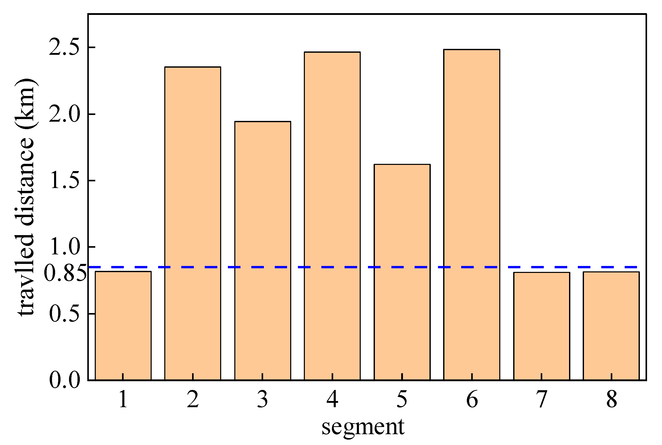
It can be seen from Table 4 that the predicted speed results of the improved GRU vehicle speed predictor, which incorporates the standard deviation of the deviation in acceleration time proportion, achieve energy reduction in segments 2 to 6. The maximum energy saving in segment 2 is 13.75 g, with an energy-saving rate of 17.45% compared to the GRU vehicle speed predictor, and the increase in execution energy consumption of the improved GRU compared to the GRU execution energy consumption relative to the theoretical optimal energy consumption is 43.18%. However, in segments 1, 7, and 8, the predicted speed results of the improved GRU vehicle speed predictor did not reduce the final energy consumption but increased it instead. Further analysis was conducted in combination with the mileage characteristics of each segment, and the mileage characteristics of each segment are shown in Figure 13.

Figure 13. Mileage statistics of different driving segments.

It can be seen from Figure 13 that the driving mileage of segments 2 to 6 is more than 1.5 km, while the driving mileage of segments 1, 7, and 8 is less than 0.85 km. For short-distance segments such as segments 1, 7, and 8, the instantaneous fluctuation of vehicle speed directly affects the final energy consumption result, and the standard deviation of the deviation in acceleration time proportion may not fully consider the energy consumption of these instantaneous fluctuations, ultimately leading to higher execution energy consumption of the improved GRU. In contrast, in other segments with longer mileage, the application of the improved GRU vehicle speed predictor incorporating the standard deviation of the deviation in acceleration time proportion can achieve energy reduction. This indicates that the standard deviation of the deviation in acceleration time proportion can not only effectively evaluate the application results of predicted speed curves but also improve the performance of predictors for longer mileage vehicle speed prediction, thus being a more effective evaluation indicator.

The acceleration time proportion, as an evaluation indicator, shows obvious advantages over traditional indicators, providing support for further research on the effectiveness of evaluation indicators. However, it is evident that the acceleration time proportion still has shortcomings as an evaluation indicator. Therefore, the development of evaluation indicators with stronger adaptability and effectiveness requires extensive and continuous exploration.

4. Conclusions

In this study, vehicle speed predictors and powertrain energy management strategies were constructed based on multiple complete driving speed profiles. By performing vehicle speed prediction and corresponding energy management optimization, predicted speed curves and their relative energy consumption deviations from theoretical optimal performance were obtained. On this basis, statistical indicators, similarity indicators, and vehicle speed characteristic indicators were calculated, and their correlations with energy consumption deviation were systematically analyzed. The main conclusions are summarized as follows.

First, traditional statistical evaluation metrics such as RMSE and MAE exhibit weak correlation with relative energy consumption deviation when predicted speed curves are applied to hybrid energy management. This indicates that numerical prediction accuracy alone is insufficient to reflect the actual effectiveness of vehicle speed prediction in energy consumption optimization. In contrast, vehicle speed characteristic indicators related to dynamic behavior show stronger correlation with energy consumption deviation, highlighting their greater relevance to energy management performance.

Second, comparative trend analysis further demonstrates that characteristic indicators reflecting acceleration behavior exhibit consistent variation trends with relative energy consumption deviation, whereas RMSE and MAE fail to capture such consistency. This result confirms that indicators describing speed variation characteristics are more suitable for evaluating the application effectiveness of predicted speed profiles in predictive energy management contexts.

Finally, incorporating the proposed characteristic indicator into the construction and optimization of vehicle speed predictors leads to improved energy consumption performance, particularly in long-distance driving scenarios. This further verifies the practical value of application-oriented evaluation indicators and suggests that vehicle speed prediction models optimized using energy-management-relevant indicators can achieve more effective energy savings.

Overall, the results indicate that the evaluation of vehicle speed prediction should be closely aligned with its target application. For predictive energy management, indicators that capture dynamic speed characteristics provide a more meaningful and effective assessment than conventional distance-based statistical metrics. This application-oriented evaluation perspective enables a more accurate reflection of the actual contribution of predicted speed profiles to energy consumption optimization.

Despite the demonstrated effectiveness of the proposed evaluation indicator, limitations remain. Its evaluation performance degrades in short-distance driving segments, and the applicable threshold range requires further clarification. Moreover, the current framework evaluates indicators independently and does not support multi-indicator integration or adaptive selection across different driving scenarios. Future work will therefore focus on determining effective threshold ranges using large-scale driving data and developing a multi-scenario adaptive evaluation framework that integrates multiple or hybrid indicators, thereby enhancing the robustness and general applicability of vehicle speed prediction effectiveness evaluation in predictive energy management.

References

1. Hou, J.; Yao, D.; Wu, F.; Shen, J.; Chao, X. Online Vehicle Velocity Prediction Using an Adaptive Radial Basis Function Neural Network. IEEE Trans. Veh. Technol. 2021, 70, 3113–3122. [Google Scholar] [CrossRef] [Scilit]
2. Zhang, H. Research and Implementation of Road Speed Prediction Algorithm Based on Deep Learning. Master’s thesis, Beijing University of Posts and Telecommunications, Beijing, China, 2020. [Google Scholar]
3. Huang, W.; Song, G.; Hong, H.; Xie, K. Deep Architecture for Traffic Flow Prediction: Deep Belief Networks With Multitask Learning. IEEE Trans. Intell. Transp. Syst. 2014, 15, 2191–2201. [Google Scholar] [CrossRef] [Scilit]
4. Lin, C.-C.; Wang, M.-S. Vehicle speeding early warning model using frame feature detection and HMM. In Proceedings of the 2011 IEEE 15th International Symposium on Consumer Electronics (ISCE), Singapore, 14–17 June 2011; pp. 241–244. [Google Scholar] [CrossRef] [Scilit]
5. Feng, Y.; Chen, T.; Li, Y.; Gao, Y.; Zhang, G.; Cao, G. Short-Term Vehicle Speed Prediction Based on Spatio-Temporal Traffic Graph Networks. IEEE Access 2025, 13, 43557–43571. [Google Scholar] [CrossRef] [Scilit]
6. Qi, L.; Zhang, J.; Jiao, X. Predecessor speed prediction-based predictive cruise control of connected autonomous vehicle in platoon with multiple-human-driven-vehicles. Control Eng. Pract. 2025, 158, 106286. [Google Scholar] [CrossRef] [Scilit]
7. Kadechkar, A.; Llauradó, X. AI-Enhanced Velocity Prediction for Efficient EV Energy Management with Hybrid Storage. In Proceedings of the 2024 12th International Conference on Smart Grid (icSmartGrid), Setubal, Portugal, 27–29 May 2024; pp. 659–665. [Google Scholar] [CrossRef] [Scilit]
8. Karunasingha, D.S.K. Root mean square error or mean absolute error? Use their ratio as well. Inf. Sci. 2022, 585, 609–629. [Google Scholar] [CrossRef] [Scilit]
9. Lei, H.; Chong, B.; Li, K. MPC Based Optimal Energy Management of Electrical Vehicles with Hybrid Energy Storage on Fixed Routine. In Proceedings of the 2025 IEEE/AIAA Transportation Electrification Conference and Electric Aircraft Technologies Symposium (ITEC+EATS), Anaheim, CA, USA, 18–20 June 2025; pp. 1–6. [Google Scholar] [CrossRef] [Scilit]
10. Lin, B.; Wei, C.; Feng, F. A Vehicle Velocity Prediction Method with Kinematic Segment Recognition. Appl. Sci. 2024, 14, 5030. [Google Scholar] [CrossRef] [Scilit]
11. Deng, Y.; Zhang, L.; Chen, J.; Deng, Y.; Liu, J. Pedestrian Trajectory Prediction Based on an Intention Randomness Influence Strategy. Electronics 2024, 13, 2008. [Google Scholar] [CrossRef] [Scilit]
12. Zhao, H.; Kou, Y.; Xue, Y.; Wang, S.; Gu, Z. TiFSN: A wavelet-EC-TCN model for quadrotor UAV trajectory prediction based on time–frequency–spatial feature fusion. Perform. Eval. 2025, 170, 102515. [Google Scholar] [CrossRef] [Scilit]
13. Kim, D.; Khalil, A.; Nam, H.; Kwon, J. OPEMI: Online Performance Evaluation Metrics Index for Deep Learning-Based Autonomous Vehicles. IEEE Access 2023, 11, 16951–16963. [Google Scholar] [CrossRef] [Scilit]
14. Chai, T.; Draxler, R.R. Root mean square error (RMSE) or mean absolute error (MAE)?—Arguments against avoiding RMSE in the literature. Geosci. Model Dev. 2014, 7, 1247–1250. [Google Scholar] [CrossRef] [Scilit]
15. Jin, Y.; Chen, T.; Chen, D.; Gao, Y. A Predictive PHEV Energy Management Strategy Based on GRU and Enhanced Dynamic Programming. In Proceedings of the 2022 6th CAA International Conference on Vehicular Control and Intelligence (CVCI), Nanjing, China, 28–30 October 2022; pp. 1–6. [Google Scholar] [CrossRef] [Scilit]
16. Zhao, Y.; Xu, L.; Zhao, C.; Xu, H.; Yan, X. Research on Energy Management Strategy for Hybrid Tractors Based on DP-MPC. Energies 2024, 17, 3924. [Google Scholar] [CrossRef] [Scilit]
17. Feng, G.; Feng, Z.; Sun, P.; Guo, L.; Chen, Z. A Overview of Energy Management Strategies for Hybrid Power Systems. Energies 2025, 18, 4769. [Google Scholar] [CrossRef] [Scilit]
18. Richalet, J.; Rault, A.; Testud, J.L.; Papon, J. Model predictive heuristic control: Applications to industrial processes. Automatica 1978, 14, 413–428. [Google Scholar] [CrossRef] [Scilit]
19. Schober, P.; Boer, C.; Schwarte, L.A. Correlation Coefficients: Appropriate Use and Interpretation. Anesth Analg. 2018, 126, 1763–1768. [Google Scholar] [CrossRef] [Scilit] [PubMed]
20. Liu, P.; Wang, S.; Zhao, P. Robust estimation and test for Pearson’s correlation coefficient. Random Matrices Theory Appl. 2024, 13, 2450023. [Google Scholar] [CrossRef] [Scilit]
Disclaimer/Publisher’s Note: The statements, opinions and data contained in all publications are solely those of the individual author(s) and contributor(s) and not of MDPI and/or the editor(s). MDPI and/or the editor(s) disclaim responsibility for any injury to people or property resulting from any ideas, methods, instructions or products referred to in the content.
Article Metrics
Citations
Article Access Statistics
Multiple requests from the same IP address are counted as one view.