Prediction-Assisted Control of an Electric-Vehicle CO₂ Heat Pump with Secondary Throttling Based on a Bidirectional Feedforward Neural Network

Abstract

To improve the low-temperature heating performance of electric-vehicle CO₂ heat pumps, their system configurations and control strategies have become increasingly complex. This has made coordinated regulation among multiple components more difficult and can lead to delayed supply-air temperature response, operating fluctuations, and other problems. Accordingly, this study proposes a shared-parameter bidirectional feedforward neural network (BFNN)-assisted regulation method. The method jointly learns the forward and inverse relationships between controllable components and the prediction variable. The inverse path generates candidate operating parameters, which are verified and corrected by the forward path to improve regulation efficiency. Under a −20 °C cold-start condition, the BFNN-assisted strategy achieved a supply-air temperature stabilization time of 8.2 min, 45.6% and 56.3% shorter than those of unidirectional FNN-assisted control and conventional rule-based feedback control, respectively. Compared with rule-based feedback control, the time-averaged heating COP over the 30 min test increased by 8.9%, while compressor energy consumption decreased by 19.0%. When cabin-side airflow increased from 300 to 550 m³/h, the BFNN-assisted strategy limited the maximum temperature drop to 2.50 °C and the recovery time to 1.67 min. Under the tested conditions, the integrated BFNN-assisted control strategy improved the CO₂ heat pump system temperature-response and energy-performance metrics.

1. Introduction

In low-temperature environments, electric vehicles cannot utilize engine waste heat, and the energy required for cabin heating is therefore supplied mainly by the traction battery. Consequently, the heating rate and operating efficiency of the heat pump system directly affect passenger thermal comfort and vehicle driving range [1,2]. CO₂, as the reference greenhouse gas, has a 100-year global warming potential (GWP₁₀₀) of 1, a high volumetric heating capacity, and a transcritical heat-rejection process that is well matched to air-heating requirements. These characteristics make it a promising refrigerant for heat pump air-conditioning systems in electric vehicles [3]. However, low ambient temperatures still deteriorate heat transfer on the outdoor side and increase the system pressure ratio, discharge temperature, and compressor power consumption. As a result, matching the refrigerant flow rate and pressure distribution with the heat transfer process becomes more difficult [4,5].

To further improve the low-temperature heating performance of CO₂ heat pumps for electric vehicles, previous studies have modified the cycle configuration and operating modes through vapor injection [6,7], refrigerant mixtures [8], charge optimization [9], and multiple evaporation temperatures combined with heat recovery [10]. These methods can improve refrigerant supply, pressure distribution, and heat transfer matching. However, the additional branches, valves, and intermediate states also introduce more adjustable operating parameters, resulting in more complex nonlinear coupling among the compressor, electronic expansion valves, and air-side parameters [11,12]. When the ambient temperature, airflow rate, or supply-air temperature target changes, uncoordinated adjustment of the compressor speed and valve openings can readily cause supply-air temperature overshoot, pressure fluctuations, frequent actuator movements, and increased energy consumption during transient operation [13,14]. Therefore, the compressor speed and the openings of the two electronic expansion valves must be coordinated rapidly and stably when air-side conditions or supply-air temperature targets change. This regulation should also satisfy operational safety constraints and reduce energy consumption. It is therefore important for the further engineering application of CO₂ heat pump systems in electric vehicles.

Existing heat pump control methods mainly include empirical rule-based control, PID control, fuzzy control, physics-based model control, and model predictive control [15,16]. Empirical rule-based and conventional feedback control methods have simple structures and are easy to implement [17]. However, they usually adjust the compressor speed and valve openings gradually according to local temperature or pressure errors. Their ability to account for multivariable coupling is therefore limited. Under low-temperature start-up and large operating-condition changes, these methods can suffer from delayed responses and repeated trial-and-error adjustments [18,19]. Model predictive control can explicitly account for multivariable constraints and future system responses. However, its control performance depends on model accuracy. Online receding-horizon optimization also increases the real-time computational burden of the controller [20,21].

Data-driven methods, such as neural networks, have gradually been applied to the performance prediction and assisted control of heat pump systems [22,23]. Feedforward neural networks can approximate the nonlinear mapping among air-side conditions, operating parameters, and system responses without repeatedly solving complex physics-based equations [24]. However, existing studies have mainly focused on unidirectional tasks that predict temperature, pressure, or energy efficiency from operating parameters [25]. When only a forward model is used, searching or optimization over a wide range of operating parameters is still required to determine the parameters corresponding to the target state [26,27]. An inverse model can rapidly estimate the operating parameters required for a target state, thereby narrowing the online search range. However, this mapping is often non-unique. Directly applying the model output may cause the operating parameters to exceed their allowable ranges or change abruptly because of model errors or insufficient sample coverage. It may also drive the system close to its safety limits. Therefore, a heat pump regulation model is still needed to jointly represent the forward and inverse relationships between operating parameters and supply-air temperature. The model should also incorporate operating-range checks and corrections based on measured feedback.

Existing neural network-based and prediction-assisted heat pump control studies generally use data-driven models to predict system performance or operating states, followed by a separate search or optimization procedure to determine suitable control parameters [28,29]. In contrast, the proposed BFNN jointly learns the forward and inverse mappings through shared hidden-layer parameters. The inverse path generates target-oriented candidate operating parameters, while the forward path evaluates their predicted thermal response before implementation. This integration combines inverse initialization, forward verification, and measured-feedback correction within a unified framework, thereby reducing repeated trial-and-error adjustment during multi-parameter regulation.

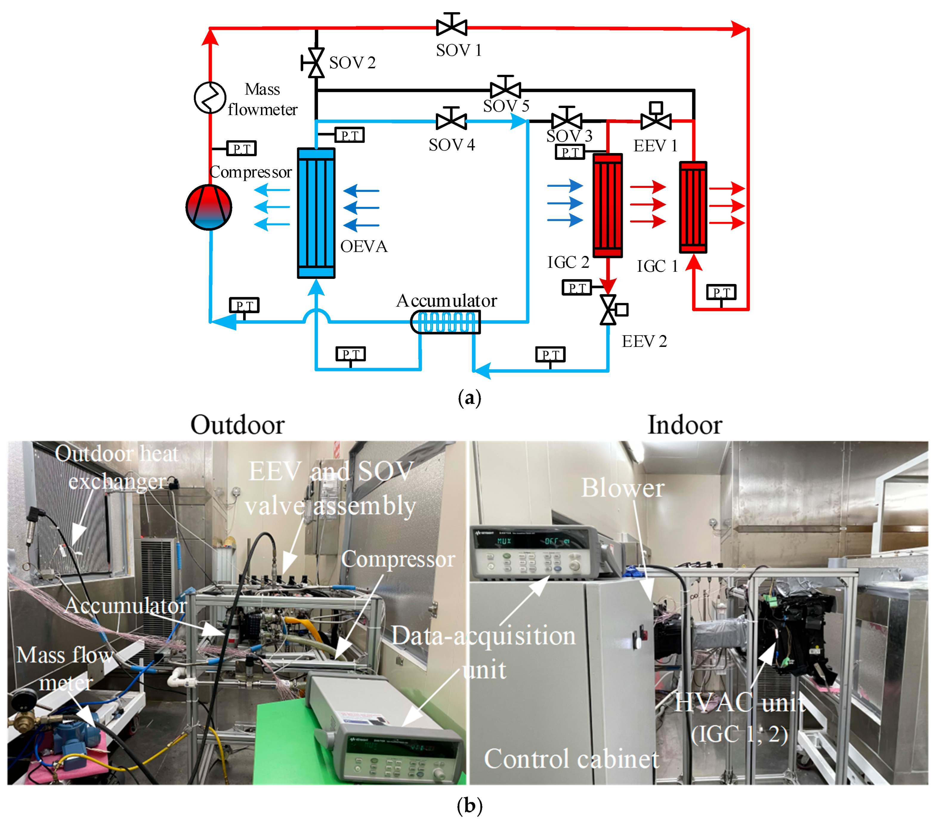
In summary, this study builds on the previously developed experimental platform for a single-stage compression CO₂ heat pump with secondary throttling [30,31]. A prediction-assisted control method based on a shared-parameter bidirectional feedforward neural network (BFNN) is proposed. The BFNN learns the forward and inverse mappings within a unified framework. The forward path estimates the supply-air temperature corresponding to each candidate combination of operating parameters based on the air-side conditions, compressor speed, and expansion valve openings. The inverse path generates candidate operating parameters based on the target supply-air temperature and the air-side conditions. The shared hidden layer extracts thermodynamic coupling features common to both tasks and reduces parameter duplication caused by separate modeling. During regulation, the inverse prediction results are used as the initial candidate operating parameters. The forward path rapidly evaluates different combinations of operating parameters. The final parameter combination for system regulation is then obtained by applying operating-parameter constraints, measured feedback, and local corrections. Accordingly, the main innovations and contributions of this study are as follows:

(1) A shared-parameter BFNN is proposed for a secondary-throttling CO₂ heat pump. It integrates the forward prediction from operating parameters to supply-air temperature and the inverse estimation from the target supply-air temperature to compressor speed and the openings of the two valves within a single model. This allows the forward and inverse tasks to reuse shared thermally coupled features and reduces redundant training caused by separate modeling.

(2) A prediction-assisted regulation mechanism comprising “inverse generation–forward evaluation–constraint-based correction” is developed. The inverse outputs are used as candidate initial values and are corrected through forward verification of the quasi-steady-state supply-air temperature, operating-range constraints, and measured feedback, thereby reducing repeated adjustments during coordinated multi-component regulation.

(3) It is verified that BFNN-assisted regulation can reduce repeated adjustments of the compressor and throttling valves, thereby improving pressure variation within the cycle, accelerating attainment of the supply-air temperature target and steady-state recovery under disturbance conditions, while improving the energy efficiency of the heat pump.

2. Experimental System and Control Problem

2.1. Secondary-Throttling CO₂ Heat Pump System and Experimental Platform

Figure 1a shows the refrigerant circuit and main measurement points of the single-stage compression CO₂ heat pump with secondary throttling. The high- and low-pressure lines are indicated in red and blue, respectively. Figure 1b shows the heat pump circuit, HVAC unit, blower, data acquisition unit, and control cabinet of the experimental platform. In heating mode, the refrigerant is compressed, releases heat to the cabin-side air through the indoor heat exchanger, undergoes secondary throttling through EEV1 and EEV2 for flow and pressure regulation, absorbs heat from the outdoor air, and then returns to the compressor. The compressor speed and the openings of EEV1 and EEV2 are the primary adjustable operating parameters. The experiments were conducted under specified air-side boundary conditions while the compressor speed and valve openings were adjusted and temperature, pressure, refrigerant mass flow rate, and compressor power were measured. Quasi-steady data were used for model development and testing, and transient tests were used for control-performance evaluation. Detailed specifications of the experimental apparatus and procedures are available in our previous studies [30,31]. Model training, independent testing, and control-performance validation in this study were all conducted using the experimental platform.

2.2. Adjustable Operating Parameters and Constraints

To ensure consistent variable definitions for model training and regulation, this section sequentially introduces the air-side operating conditions, compressor and electronic expansion valve setpoints, forward and inverse models, supply-air temperature target, and safety constraints. Equation (1) defines the air-side operating conditions and operating-parameter setpoints for the k regulation cycle. Equation (2) specifies the inputs and outputs of the forward and inverse models. Equation (3) gives the supply-air temperature deviation and the criterion for retaining the current setpoints. Equation (4) defines the allowable ranges of the compressor speed and valve openings, together with the safe operating limits.

$$d_k={\left[T_{\mathrm{out},k},T_{\mathrm{in},k},v_{\mathrm{out},k},V_{\mathrm{in},k}\right]}^{\mathrm{T}},u_k={\left[N_{\mathrm{com},k},O_{1,k},O_{2,k}\right]}^{\mathrm{T}}$$

(1)

where d_k is the measurable air-side boundary-state vector at control interval k; u_k is the operating-parameter vector; T_out,k and T_in,k are the outdoor-air temperature and the cabin-side heat-exchanger inlet-air temperature, respectively; v_out,k is the face velocity of the outdoor heat exchanger; V_in,k is the cabin-side volumetric airflow rate; N_com,k is the compressor speed; O_1,k and O_2,k are the openings of EEV1 and EEV2, respectively; and the superscript T denotes transpose.

$$\begin{array}{l}{x}_{f,k}={\left[d_k^{\mathrm{T}},u_k^{\mathrm{T}}\right]}^{\mathrm{T}},y_{f,k}=T_{\sup ,k}\\ x_{r,k}={\left[d_k^{\mathrm{T}},T_{r,k}\right]}^{\mathrm{T}},y_{r,k}=u_k\end{array}$$

(2)

where $x_{f,k}$ and $y_{f,k}$ are the input and target output of the forward mapping, respectively; $x_{r,k}$ and $y_{r,k}$ are the input and target output of the inverse mapping, respectively; $T_{r,k}$ denotes the reference supply-air temperature, which is given by the measured supply-air temperature during offline training and replaced by the target supply-air temperature during online control; and the remaining symbols are defined in Equation (1).

$$e_{T,k}=T_{\sup ,k}-T_{\mathrm{set},k},\left|e_{T,k}\right|\le {0.25}^{\circ }\mathrm{C}$$

(3)

where e_T,k is the supply-air temperature tracking error; T_sup,k denotes the measured supply-air temperature; T_set,k is the corresponding target temperature; and 0.25 °C is the online termination threshold used to maintain the current control command.

$$\begin{array}{l}{u}_{\min }\le u_k\le u_{\max },\left|u_k-u_{k-1}\right|\le \Delta u_{\max }\\ P_{dis,k}\le 10\mathrm{MPa},T_{dis,k}\le 135°\mathrm{C}\end{array}$$

(4)

where u_min and u_max are the lower and upper bounds of the operating-parameter vector, respectively; u_k and u_k−1 are the operating-parameter vectors at the current and previous control intervals; Δu_max is the allowable single-interval operating-parameter variation; and P_dis,k and T_dis,k are the measured discharge pressure and discharge temperature used as post-adjustment hard safety limits. The optimal intermediate-pressure relationship is applied after parameter adjustment through measured feedback and is not included in the allowable pre-adjustment operating range.

The forward model estimates the quasi-steady-state supply-air temperature corresponding to a given combination of air-side operating conditions and operating parameters. It does not describe the thermal inertia or the state evolution of the system. In prediction-assisted regulation, the model is used to rapidly evaluate candidate steady-state operating points. Dynamic deviations are then compensated through measured supply-air temperature feedback and constrained parameter adjustments. The inverse model estimates the compressor speed and the openings of the two valves from the air-side operating conditions and the target supply-air temperature. Because the same supply-air temperature may correspond to multiple combinations of operating parameters, its outputs are used only as initial values for candidate operating parameters and cannot be directly applied as the final setpoints.

The supply-air temperature is the primary regulation target. When its absolute deviation does not exceed 0.25 °C, the current operating-parameter setpoints are retained. Dynamic performance is evaluated by the time required for the supply-air temperature to enter and remain within the ±0.50 °C target band. For the secondary-throttling system, pressure distribution is coordinated with the aid of the optimal intermediate-pressure relationship established from experimental data in our previous studies [30,31].

3. Shared-Parameter Bidirectional Feedforward Neural Network and Prediction-Assisted Control

3.1. Forward and Inverse Prediction with the BFNN

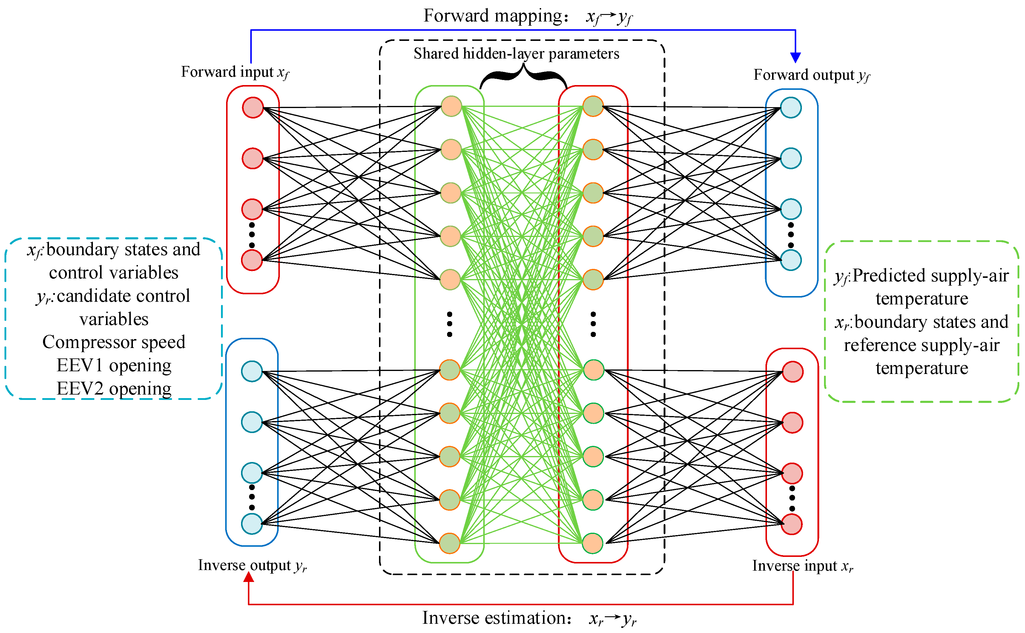
Figure 2 shows the shared-parameter BFNN architecture. The forward path takes the air-side operating conditions, compressor speed, and openings of the two electronic expansion valves as inputs and predicts the corresponding quasi-steady-state supply-air temperature. The inverse path takes the air-side operating conditions and target supply-air temperature as inputs and estimates the compressor speed and the openings of the two valves. The two paths have separate input and output layers but share the parameters of the intermediate hidden layers. This enables forward prediction and inverse estimation tasks to reuse the common thermodynamic coupling features among the air-side operating conditions, operating parameters, and supply-air temperature.

This architecture does not simply place two independent networks in parallel; instead, it jointly learns the forward and inverse mappings within a unified parameter framework. Because the same supply-air temperature may correspond to multiple combinations of compressor speed and valve openings, the outputs of the inverse path are used only as candidate operating parameters rather than directly as the final setpoints. The candidate parameters are further evaluated using the forward prediction of supply-air temperature and corrected according to the operating-range constraints and measured feedback to obtain an operating-parameter combination suitable for the current conditions. Therefore, the BFNN is not intended to directly replace feedback control. Instead, it narrows the search range of the operating parameters and provides more reasonable initial values for regulation, thereby reducing repeated adjustments of the compressor and the two valves while improving the response speed and stability of supply-air temperature regulation.

3.2. Mathematical Formulation and Training Parameters

The forward and inverse paths of the BFNN are expressed in Equation (5):

$$\begin{array}{l}{\widehat{T}}_{\sup ,k}=F\left(x_{f,k};{\theta }_f,{\theta }_s\right)\\ {\widehat{u}}_k=G\left(x_{r,k};{\theta }_r,{\theta }_s\right)\end{array}$$

(5)

where ${\widehat{T}}_{\mathrm{s}\mathrm{u}\mathrm{p},k}$ is the supply-air temperature predicted by the forward mapping; ${\widehat{u}}_k$ is the candidate operating-parameter vector estimated by the inverse mapping; $F\left(\cdot \right)$ and $G\left(\cdot \right)$ denote the forward and inverse network functions, respectively; ${\theta }_f$ and ${\theta }_r$ are the path-specific parameters; and ${\theta }_s$ denotes the shared hidden-layer parameters.

The shared features are calculated using Equation (6). The shared parameters receive gradients from both the forward and inverse losses, enabling the two paths to learn the common thermodynamic coupling relationships among the air-side operating conditions, compressor speed, valve openings, and supply-air temperature through the shared hidden layers.

$$h_{q,k}^{(l)}=\mathrm{ReLU}\left(W_s^{(l)}{h}_{q,k}^{(l-1)}+b_s^{(l)}\right),q\in \{f,r\}$$

(6)

where $h_{q,k}^{\left(l\right)}$ is the feature representation of direction $q$ at shared hidden layer $l$; $q=f$ and $q=r$ denote the forward and inverse directions, respectively; $W_s^{\left(l\right)}$ and $b_s^{\left(l\right)}$ are the shared weight matrix and bias vector; and $\mathrm{R}\mathrm{e}\mathrm{L}\mathrm{U}\left(\cdot \right)$ denotes the rectified linear unit activation function.

The BFNN is trained using the joint forward–inverse loss defined in Equation (7). The task-specific parameters of the forward and inverse paths are updated by their respective losses, whereas the shared parameters are jointly updated by both losses. Because the inverse mapping may yield multiple feasible combinations of operating parameters, its outputs are used only as initial operating parameters for online regulation.

$$\begin{array}{l}{L}_f={\displaystyle \frac{1}{N_{\mathrm{tr}}}}{\displaystyle \sum _{i=1}^{N_{\mathrm{tr}}}{\left({\widehat{T}}_{\sup ,i}-T_{\sup ,i}\right)}^2}\\ L_r={\displaystyle \frac{1}{3N_{\mathrm{tr}}}}{\displaystyle \sum _{i=1}^{N_{\mathrm{tr}}}{‖{\widehat{u}}_i-u_i‖}_2^2}\\ L=Lf+Lr\end{array}$$

(7)

where $L_f$ is the mean squared error of the standardized supply-air temperature; $L_r$ is the mean squared error averaged over the three standardized operating parameters; $N_{\mathrm{t}\mathrm{r}}$ is the number of training samples; and $L$ is the joint bidirectional training loss. The measurable boundary variables are used only as conditional inputs and are not included in either prediction loss.

To prevent data leakage, the mean and standard deviation are calculated using only the training set and are then applied consistently to all three data subsets. The ith sample of the jth variable is standardized and inverse-transformed according to Equation (8). Before error calculation and the generation of actual operating parameters, the model outputs are restored to their original physical units.

$$\begin{array}{l}{z}_{i,j}={\displaystyle \frac{q_{i,j}-{\mu }_{j,\mathrm{tr}}}{{\sigma }_{j,\mathrm{tr}}}}\\ q_{i,j}={\mu }_{j,\mathrm{tr}}+{\sigma }_{j,\mathrm{tr}}{z}_{i,j}\end{array}$$

(8)

where q_i,j and z_i,j are the original and standardized values of variable j in sample i, respectively; μ_j,tr and σ_j,tr are the mean and standard deviation of variable j calculated exclusively from the training set.

The candidate operating-parameter evaluation defined in Equation (9) considers both the predicted supply-air temperature error and the smoothness of changes in the compressor speed and valve openings. D_u is the diagonal scaling matrix constructed from the allowable ranges of the compressor speed and the openings of the two valves, and λ_Δ is the penalty coefficient for changes in the operating parameters. Before actual regulation, the allowable operating range includes only constraints on the magnitudes of the operating parameters and their rates of change per regulation cycle. The pressure and discharge-temperature thresholds are used as measured safety criteria after regulation for feedback correction and independent protection.

$$\underset{u_k\in U}{\min }J\left(u_k\right)=\left|{\widehat{T}}_{\sup ,k}-{\mathrm{T}}_{\mathrm{set},\mathrm{k}}\right|+{\lambda }_{\Delta }{‖D_u^{-1}\left(u_{\mathrm{k}}-u_{\mathrm{k}-1}\right)‖}_2^2$$

(9)

where J(_uk) is the online candidate operating-parameter evaluation objective; U is the allowable operating-parameter set; u_k is a candidate operating-parameter vector; ${\widehat{T}}_{\mathrm{s}\mathrm{u}\mathrm{p},k}$ is the supply-air temperature predicted by the forward BFNN; T_set,k is the target supply-air temperature; λ_Δ is the operating-parameter variation penalty coefficient; D_u is the diagonal scaling matrix formed from the allowable ranges of compressor speed and two valve openings; u_k−1 is the operating-parameter vector from the previous adjustment interval.

In Equation (9), the supply-air temperature error is expressed in °C, whereas the normalized operating-parameter variation term is dimensionless. Accordingly, λ_Δ is a temperature-equivalent penalty coefficient and was set to 0.10 °C in this study. Its value was selected from preliminary sensitivity tests to prioritize supply-air temperature tracking while suppressing unnecessary operating-parameter changes.

When the temperature deviation exceeds the allowable limit, a constrained feedback adjustment is generated based on the measured temperature deviation, pressure-reference deviation, and safety status. According to Equation (10), the adjusted compressor speed and valve openings are then restricted to their allowable magnitude and single-cycle change ranges.

$$u_k\leftarrow {\prod }_{\mathrm{U}}\left(u_k^{\ast }+\Delta u_k\right)$$

(10)

where u_k is the final operating-parameter vector; $u_k^{*}$ is the optimized candidate obtained from Equation (9); Δu_k is the bounded feedback-adjustment vector generated from the current tracking error and measured state; Π_U(·) is the projection operator; and U is the allowable operating-parameter set defined only by the operating-parameter magnitude and single-interval rate constraints. The measured pressure and discharge-temperature limits are not included in this pre-adjustment constraint projection; they are handled by post-execution supervisory feedback and independent protection.

The above equations describe the bidirectional mappings, joint training, data transformation, candidate operating-parameter evaluation, and feedback correction. The corresponding settings are summarized in

Table 1. BFNN variables, operating settings and constraints in heating mode.

Category	Variables or Item	Definition and Setting	Unit
Model input and output	Forward input Inverse input	xf = [d,u] xr = [d,Tr]	—
Model input and output	Forward output Inverse output	${\widehat{T}}_{\mathrm{s}\mathrm{u}\mathrm{p}}$ u	°C; rpm; steps
Adjustable operating parameters	Ncom, EEV1 opening, EEV2 opening	Ranges: 2000–7000; 70–130; 50–110. First-update limits: 800; 25; 30. Subsequent-update limits: 300; 6; 6.	rpm; steps
Heating target	Tsup	Primary tracking variable: 35–45 °C; 40 °C for start-up; 35→40 °C for the step case	°C
Temperature criterion	Absolute tracking error; settling band	Online termination criterion ≤0.25 °C; settling-time band ±0.50 °C	°C
Safety limits and pressure-coordination reference	Pdis, Pint, Tdis	Pdis ≤ 10.0 MPa; Pint ≈ 0.88Pdis (pressure-coordination reference, not a hard safety limit); Tdis ≤ 135 °C	MPa; °C; —
Dataset	Development and test data	Quasi-steady experimental samples: 900 total; grouped by complete experimental run into 60% training, 20% validation and 20% held-out test	samples
Network	Shared feature block	Two fully connected hidden layers; 64 neurons per layer; ReLU; dropout 0.10	—
Training	Bidirectional loss and optimizer	L = Lf + Lr as defined in Equation (7); Adam; learning rate 5 × 10−4	—

.

3.3. Dataset Distribution

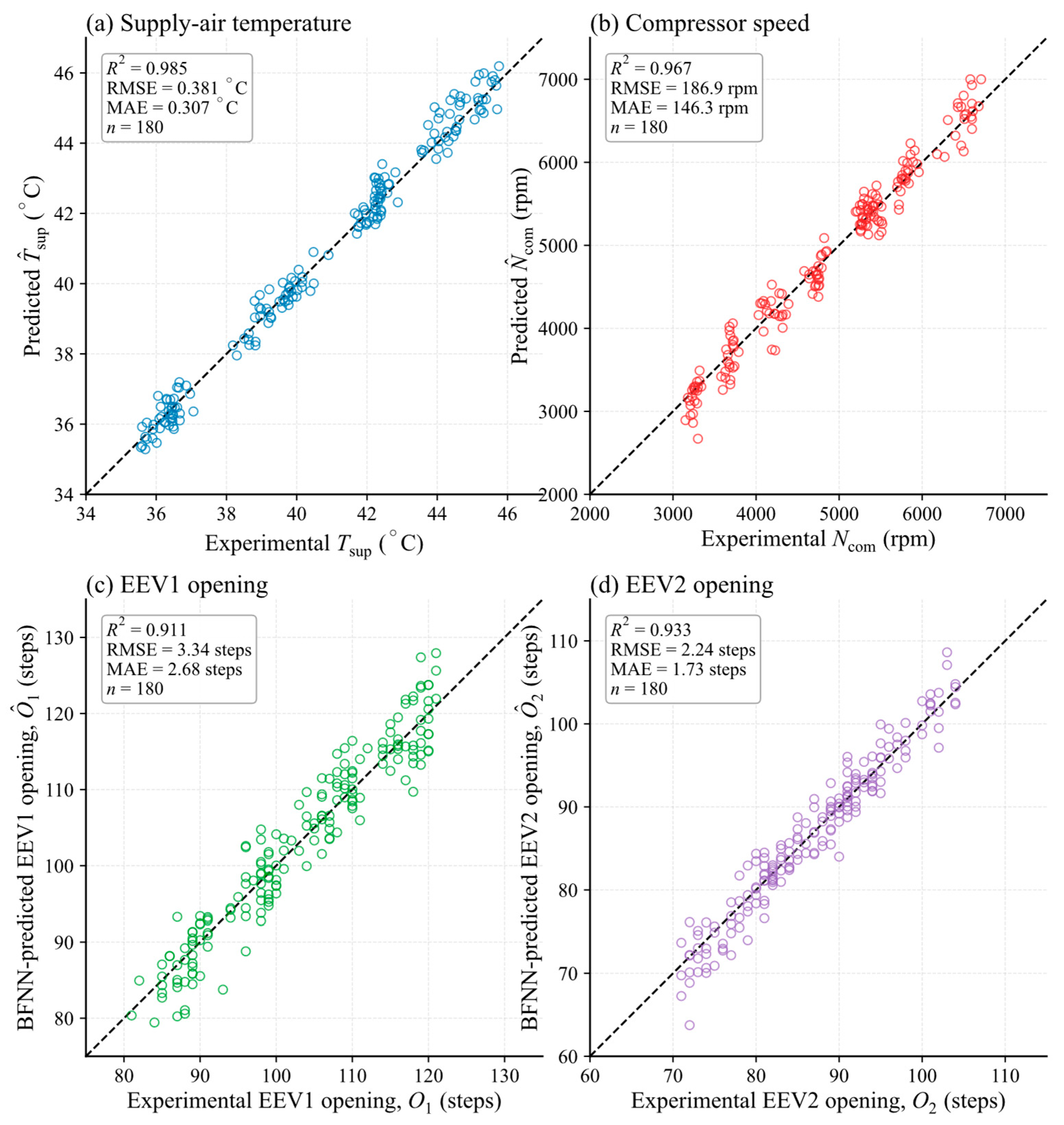
A total of 900 quasi-steady-state samples were obtained from 30 independent experimental runs, with six runs conducted at each ambient-temperature condition. After data screening, 173, 181, 176, 183, and 187 valid samples were retained at ambient temperatures of −20, −15, −10, −5, and 0 °C, respectively. The cabin-side airflow rate covered 300–550 m³/h. The compressor speed ranged from 2000 to 7000 rpm, while the openings of EEV1 and EEV2 ranged from 70 to 130 and 50 to 110 steps, respectively, with the samples distributed primarily within the intermediate operating ranges and a smaller proportion covering the boundary regions. These distributions indicate that the dataset covers the main operating range of the experimental heat pump system rather than being concentrated around a single operating point. To prevent temporally correlated samples from the same continuous experiment from being distributed across different subsets, all samples from each complete experimental run were retained within the same subset. The samples were grouped by complete experimental batch and divided into the training, validation, and test sets at ratios of 60%, 20%, and 20%, respectively, using a fixed dataset-partition seed of 42. All variables were standardized according to Equation (8), with the mean and standard deviation calculated exclusively from the training set and subsequently applied to the validation and held-out test sets. The outputs were restored to their original physical units before calculating the RMSE and MAE and generating the actual operating parameters.

3.4. Prediction-Assisted Control Method

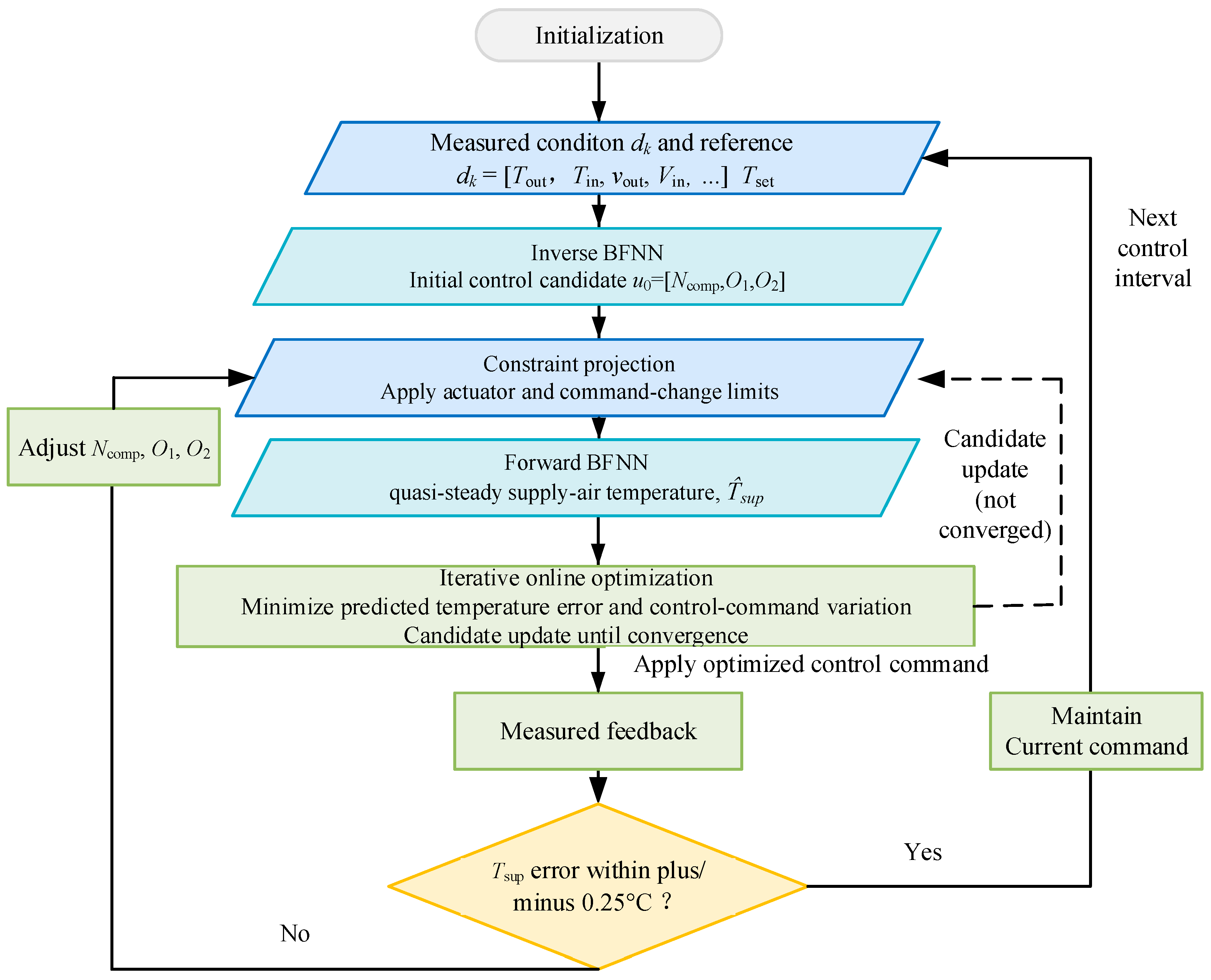
Based on the joint forward–inverse modeling described above, the BFNN is further embedded into the heat pump operating-regulation process, as shown in Figure 3. At the beginning of each regulation cycle, air-side operating conditions, including the outdoor temperature, cabin-side heat-exchanger inlet temperature, and airflow rate, are collected. These variables, together with the target supply-air temperature T_set, are input into the inverse BFNN to obtain the initial operating-parameter combination u₀ = [N_com, O₁, O₂], corresponding to the compressor speed and the openings of EEV1 and EEV2, respectively. This combination provides a candidate initial value close to the target operating condition, thereby narrowing the range of subsequent regulation and avoiding repeated trial-and-error adjustments from a fixed initial value.

After the initial operating parameters are subjected to operating-range constraints and single-cycle change limits, 27 candidate combinations are generated around the current candidate center using the Cartesian product of three discrete offsets for each operating parameter. In the first search iteration, the offsets are −300, 0, and +300 rpm for compressor speed and −6, 0, and +6 steps for both EEV1 and EEV2. If further refinement is required, the offsets are reduced to ±200 rpm and ±4 steps in the second iteration and ±100 rpm and ±2 steps in the third iteration. All candidate combinations are projected onto the allowable operating set U before evaluation. The forward BFNN then predicts the quasi-steady-state supply-air temperature for each candidate, and the candidate with the minimum objective value defined in Equation (9) is retained. The search is terminated when the predicted supply-air temperature deviation is no greater than 0.25 °C; otherwise, the best candidate is used as the center of the next refinement iteration. A maximum of three iterations is allowed. If the termination criterion is still not satisfied after the final iteration, the candidate with the minimum objective value is applied and subsequently corrected using measured feedback if necessary.

After the operating parameters are applied, the system performs feedback correction based on the measured supply-air temperature. When the supply-air temperature deviation does not exceed 0.25 °C, the current setpoints are retained and the system proceeds to the next regulation cycle. Otherwise, a small adjustment is generated according to the temperature deviation, constrained by Equation (10), and then subjected to another forward evaluation. It should be noted that the BFNN is used only to generate candidate operating parameters and evaluate the quasi-steady-state supply-air temperature. It does not predict the COP, power, pressure, or discharge temperature. The discharge pressure (P_dis), intermediate pressure (P_int), discharge temperature (T_dis), and compressor power are measured directly using sensors or a power meter. The pressure and discharge-temperature measurements are used for operating-condition monitoring and independent safety protection, whereas the COP and energy consumption are used only to evaluate the experimental results. This regulation process consists of three steps: the inverse BFNN generates candidate operating parameters, the forward BFNN evaluates the candidates and selects a suitable parameter combination, and measured feedback is used for subsequent correction when necessary. The BFNN narrows the search range while retaining the original feedback-regulation and safety-protection functions.

4. Model Performance Validation

4.1. Training and Validation Results of the Shared-Parameter Network

Figure 4 compares the validation MSE and optimal training epoch of the shared-parameter BFNN and two independent FNNs for supply-air temperature prediction and inverse estimation of the operating parameters. Each model is updated using only the training set. The fixed validation set is excluded from backpropagation, and the model corresponding to the lowest validation MSE is retained. To account for the stochastic variability associated with network initialization and optimization, both the shared-parameter BFNN and the independent FNNs were independently trained five times using different training seeds, while the dataset partition was kept fixed across all runs. The validation metrics reported in this section are expressed as the mean ± standard deviation over the five independent runs. Across the five independent runs, the minimum validation MSEs for the forward task were 0.0130 ± 0.0005 and 0.0117 ± 0.0004 for the independent FNN and BFNN, respectively, while those for the inverse task were 0.0262 ± 0.0010 and 0.0229 ± 0.0008, respectively.

The validation MSEs of both model types gradually decreased and eventually stabilized. For the representative training run shown in Figure 4, the independent FNN achieved its minimum MSE of 0.0128 at epoch 686, whereas the BFNN reached 0.0115 at epoch 1225, corresponding to an absolute reduction of 0.0013 and a relative reduction of 10.2%. For inverse estimation of the operating parameters, the minimum MSE decreased from 0.0259 to 0.0226, representing an absolute reduction of 0.0033 and a relative reduction of 12.7%. Under the same data partitioning and training settings, the shared-parameter BFNN achieved lower validation errors for both supply-air temperature prediction and operating-parameter estimation. This indicates that the shared hidden layers facilitate the reuse of thermodynamic coupling features common to the two tasks. The two independent FNNs required a total of 1386 training epochs to reach their minimum MSEs, whereas the jointly trained BFNN required 1225 epochs, corresponding to an 11.6% reduction in the cumulative number of training epochs. This result should be interpreted only as a difference in convergence behavior rather than as a direct reduction in training time or computational complexity, because the computational cost per epoch is not necessarily equivalent between the jointly trained BFNN and the standalone FNNs. The relatively high initial loss for inverse estimation of the operating parameters may be attributed to the nonlinear and non-unique mapping between the target supply-air temperature and multiple feasible operating-parameter combinations.

4.2. Prediction Performance on the Independent Test Set

To evaluate the effect of the shared architecture on prediction performance for independent test samples that were completely excluded from both training and model selection, independent FNNs for supply-air temperature prediction and inverse estimation of the operating parameters were tested using the same data partitioning. The test set was not used for parameter updating, early stopping, or model selection. The test results are presented in

Table 2. Test-set prediction performance of the independent FNNs and the shared-parameter BFNN.

Predicted Variable	FNN			BFNN
	R2	RMSE	MAE	R2	RMSE	MAE
Supply-air temperature	0.977 ± 0.004	0.470 ± 0.018 °C	0.387 ± 0.015 °C	0.985 ± 0.003	0.381 ± 0.014 °C	0.307 ± 0.012 °C
Compressor speed	0.952 ± 0.006	225.7 ± 12.4 rpm	175.1 ± 10.1 rpm	0.967 ± 0.004	186.9 ± 9.8 rpm	146.3 ± 8.3 rpm
EEV1 opening	0.877 ± 0.010	3.93 ± 0.21 steps	2.99 ± 0.18 steps	0.911 ± 0.008	3.34 ± 0.18 steps	2.68 ± 0.15 steps
EEV2 opening	0.899 ± 0.009	2.75 ± 0.17 steps	2.04 ± 0.14 steps	0.933 ± 0.007	2.24 ± 0.14 steps	1.73 ± 0.12 steps

as the mean ± standard deviation over the same five independent training runs. Figure 5 presents representative test-set prediction results from one of the five independent training runs, including the forward prediction of supply-air temperature and the inverse estimation of compressor speed and the openings of the two valves.

As shown in Table 2, the shared-parameter BFNN achieved higher R² values and lower RMSE and MAE values than the independent FNNs for all four predicted variables. The prediction points in Figure 5 generally lie close to the 1:1 line, with those for the supply-air temperature and compressor speed being more concentrated than those for the openings of EEV1 and EEV2. Within the investigated range, the former two variables exhibit more continuous and clearly defined relationships with the heating load. The two valves must be coordinated to regulate the refrigerant flow rate and pressure distribution. Multiple combinations of valve openings may therefore correspond to similar supply-air temperatures. Their discrete step positions, hysteresis, and local coupling also lead to greater dispersion in the inverse estimates.

5. Regulation Performance and Energy-Efficiency Analysis in Heat Pump Mode

5.1. Experimental Conditions and Comparison Methods

Table 3. Heating-operation cases and test settings.

Control Case	Air-Side Operating Condition	Set Point or Reference	Run Time or Update Basis
Low-temperature start-up	100% outdoor air; Tout = Tin = −20 °C; initial Tsup ≈ −18 °C	Tsup,set = 40 °C from the cold state	30 min; 10 s sampling
Supply-air temperature step	100% outdoor air; Tout = Tin = −10 °C; initially stable at Tsup = 35 °C	Tsup,set 35→40 °C at t = 1 min	15 min; 10 s sampling
Pressure-response and safety observation	100% outdoor air; inlet-air condition held constant	Reference operating point: Pdis ≈ 8.80 MPa; Pint ≈ 7.74 MPa; Pint/Pdis ≈ 0.88 [30,31]	10 s per update; convergence is confirmed by two consecutive updates within the operating-parameter stability band
Ambient-temperature comparison	100% outdoor air; Tout = Tin = 0, −5, −10, −15 and −20 °C; cabin-side airflow rate Vin = 300 m3/h	Tsup = 40 °C	30 min per case; 10 s sampling
Cabin-side airflow step disturbance	100% outdoor air; Tout = Tin = −10 °C; initially stable at Vin = 300 m3/h		20 min; 10 s sampling; 120 s moving-window heating COP

summarizes five types of heat pump regulation tests under 100% fresh-air conditions. The low-temperature start-up and supply-air temperature tests evaluate the heating-up process and supply-air temperature response. The operating-parameter and pressure-response tests examine the coordinated variations in compressor speed and valve openings, as well as pressure safety. The multi-ambient-temperature and cabin-side airflow step tests evaluate operating-condition adaptability and energy efficiency, and disturbance recovery, respectively.

Each experimental condition was repeated three times for each control strategy under the same boundary conditions and control settings. The results presented in Figure 6, Figure 7, Figure 8, Figure 9 and Figure 10 correspond to representative runs, while the repeatability of the principal performance metrics was evaluated based on the three repeated tests. Three control strategies were compared: Strategy A, conventional feedback control; Strategy B, one-way FNN-assisted control; Strategy C, BFNN-assisted control. The three strategies used the same experimental apparatus, initial conditions, target temperature, 10 s regulation cycle, allowable ranges of compressor speed and valve openings, and safety-protection settings. Strategy A uses segmented rule-based feedback. When the temperature deviation exceeds 5 °C, is between 2 and 5 °C, or is between 0.25 and 2 °C, the compressor speed is adjusted by 300, 200, or 100 rpm, respectively. The current compressor speed is maintained once the temperature enters the ±0.25 °C deadband. The two valves are coordinated according to the deviation of P_int/P_dis. The valve openings are adjusted by 4 steps when the deviation exceeds 0.02 and by 2 steps when it is between 0.01 and 0.02; they are maintained when the deviation does not exceed 0.01. Strategies B and C use the same operating-parameter search ranges, step sizes, number of candidates, candidate evaluation criterion, maximum number of iterations, and stopping conditions. Strategy B uses only the independent forward FNN and takes the operating-parameter setpoints from the previous regulation cycle as the center for candidate generation. Strategy C is the BFNN-assisted strategy. It uses the inverse-output parameter combination, after operating-range constraints are applied, as the candidate-generation center and combines shared-parameter forward evaluation with measured feedback. After the operating parameters are applied, Strategies B and C use the same segmented temperature correction, pressure coordination, operating-range constraints, and safety protection as Strategy A.

5.2. Low-Temperature Start-Up and Supply-Air Temperature Change Response

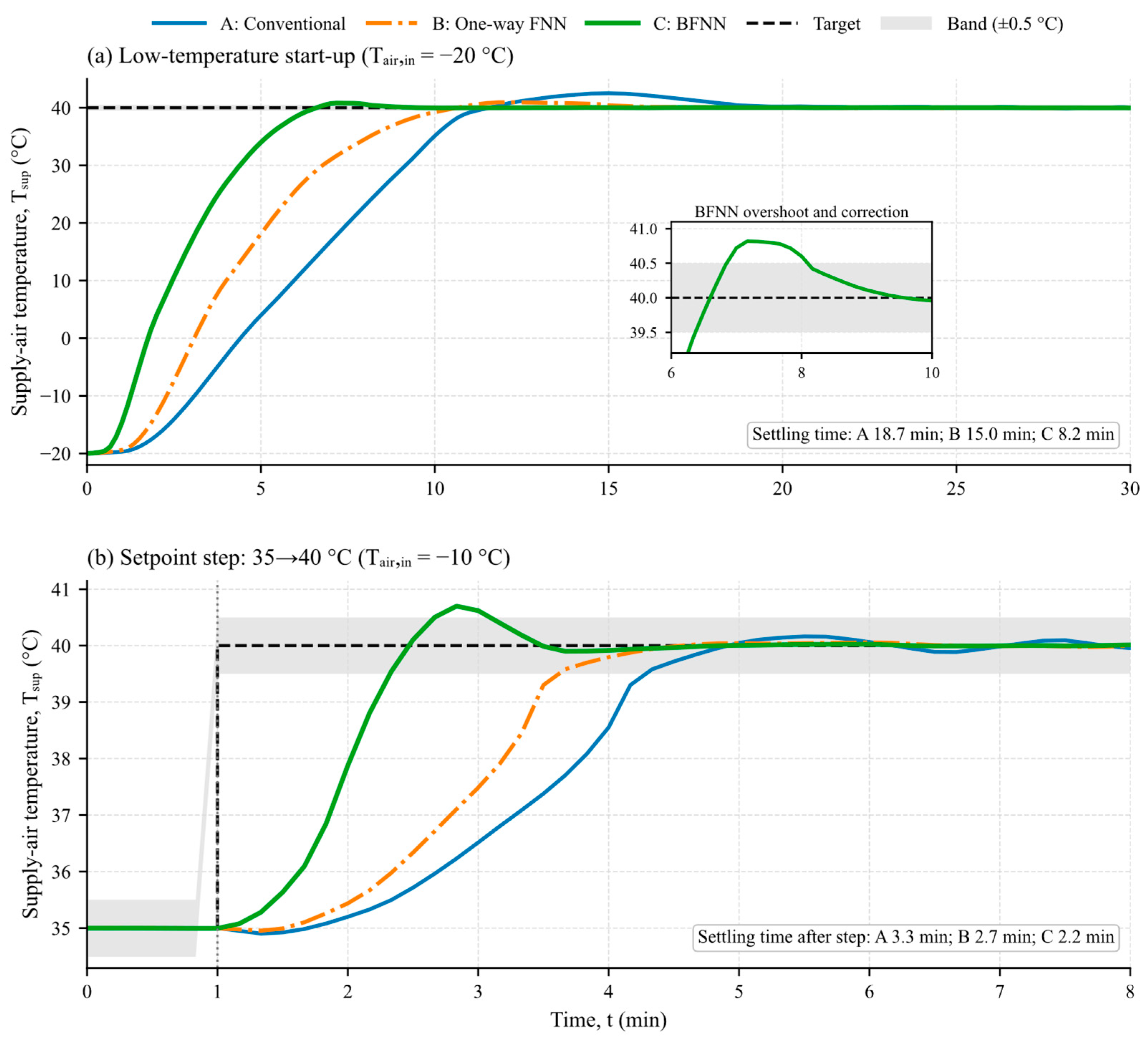
Figure 6 compares the heating-up and supply-air temperature response performance of the three strategies during a cold start under 100% fresh-air conditions at −20 °C and when the supply-air temperature setpoint is stepped from 35 to 40 °C. As shown in Figure 6a, under the −20 °C cold-start condition, the BFNN-assisted strategy achieved the fastest heating-up response, followed by the unidirectional FNN-assisted strategy, while the rule-based feedback strategy was the slowest. After a brief overshoot, the BFNN-assisted strategy was corrected through feedback and remained continuously within the 40 ± 0.50 °C band after 8.2 min. The stabilization times of the unidirectional FNN-assisted and rule-based feedback strategies were 15.0 and 18.7 min, respectively. Based on the original 10 s time series, the BFNN-assisted strategy reduced the stabilization time by 45.6% and 56.3% compared with the unidirectional FNN-assisted and rule-based feedback strategies, respectively. This improvement may result from the combined effects of inverse candidate initialization, shared-parameter forward evaluation, and measured feedback. As shown in Figure 6b, after the setpoint step change, the stabilization times of the BFNN-assisted, unidirectional FNN-assisted, and rule-based feedback strategies were 2.2, 2.7, and 3.3 min, respectively. Although the BFNN-assisted strategy exhibited a slight overshoot, it was corrected rapidly and showed no sustained oscillation after entering the allowable band. This indicates that the BFNN-assisted strategy can reach the target supply-air temperature more quickly and rapidly restore stable operation after overshoot.

5.3. Coordinated Regulation of the Compressor and Throttling Parameters

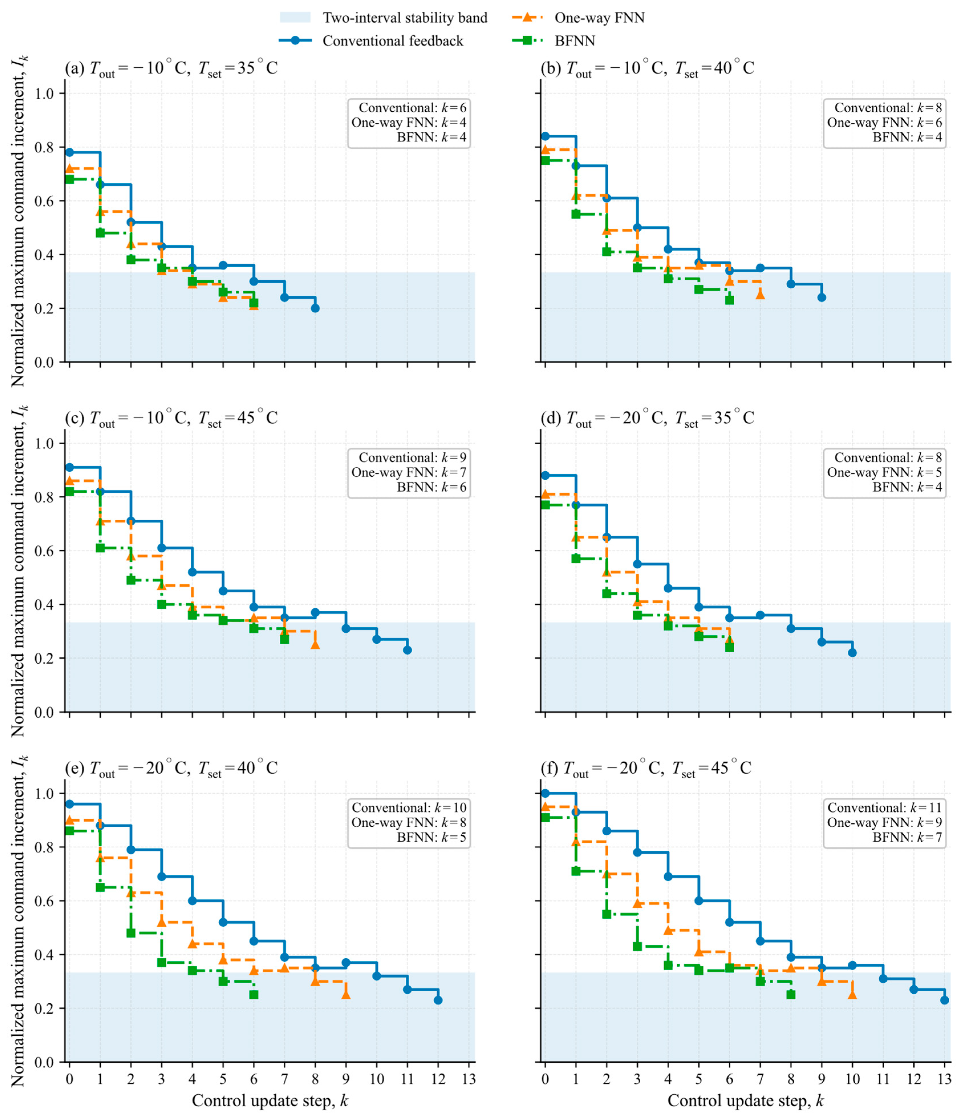
To evaluate the coordinated variations in compressor speed and valve openings under different boundary conditions and supply-air temperature targets, ambient temperatures of −10 and −20 °C were selected. Target supply-air temperatures of 35, 40, and 45 °C were set at each ambient temperature, forming six operating conditions. The results are shown in Figure 7. In the figure, ${\eta }_{\mathsf{\Delta }u,k}$ denotes the normalized maximum operating-parameter change index, which represents the parameter with the largest variation among the compressor speed, EEV1 opening, and EEV2 opening. When ${\eta }_{\mathsf{\Delta }u,k}\le 1/3$ for two consecutive regulation cycles, the compressor speed and valve openings are considered to have essentially stabilized.

For all three strategies, the magnitude of operating-parameter changes decreased as the number of updates increased. The BFNN-assisted strategy, which combines inverse initialization, shared-parameter forward evaluation, and measured feedback, achieved basic stabilization of the operating parameters earliest under most operating conditions. The unidirectional FNN-assisted strategy evaluated local candidate operating parameters using the forward model and generally converged faster than rule-based feedback. The rule-based feedback strategy gradually corrected the operating parameters according to temperature and pressure deviations, resulting in slower convergence, with plateaus or corrective reversals under some operating conditions.

At −10/35 °C, both the complete BFNN-assisted and unidirectional FNN-assisted strategies essentially stabilized after the fourth adjustment. At −10/40 °C and −20/40 °C, the BFNN-assisted strategy required four and five adjustments, respectively, which are fewer than the six and eight adjustments required by the unidirectional FNN-assisted strategy. Across the six operating conditions, the average numbers of adjustments required for the operating parameters to essentially stabilize were 5.00, 6.50, and 8.67 for the BFNN-assisted, unidirectional FNN-assisted, and rule-based feedback strategies, respectively. The BFNN-assisted strategy reduced the average number of adjustments by 23.1% and 42.3% compared with the unidirectional FNN-assisted and rule-based feedback strategies, respectively.

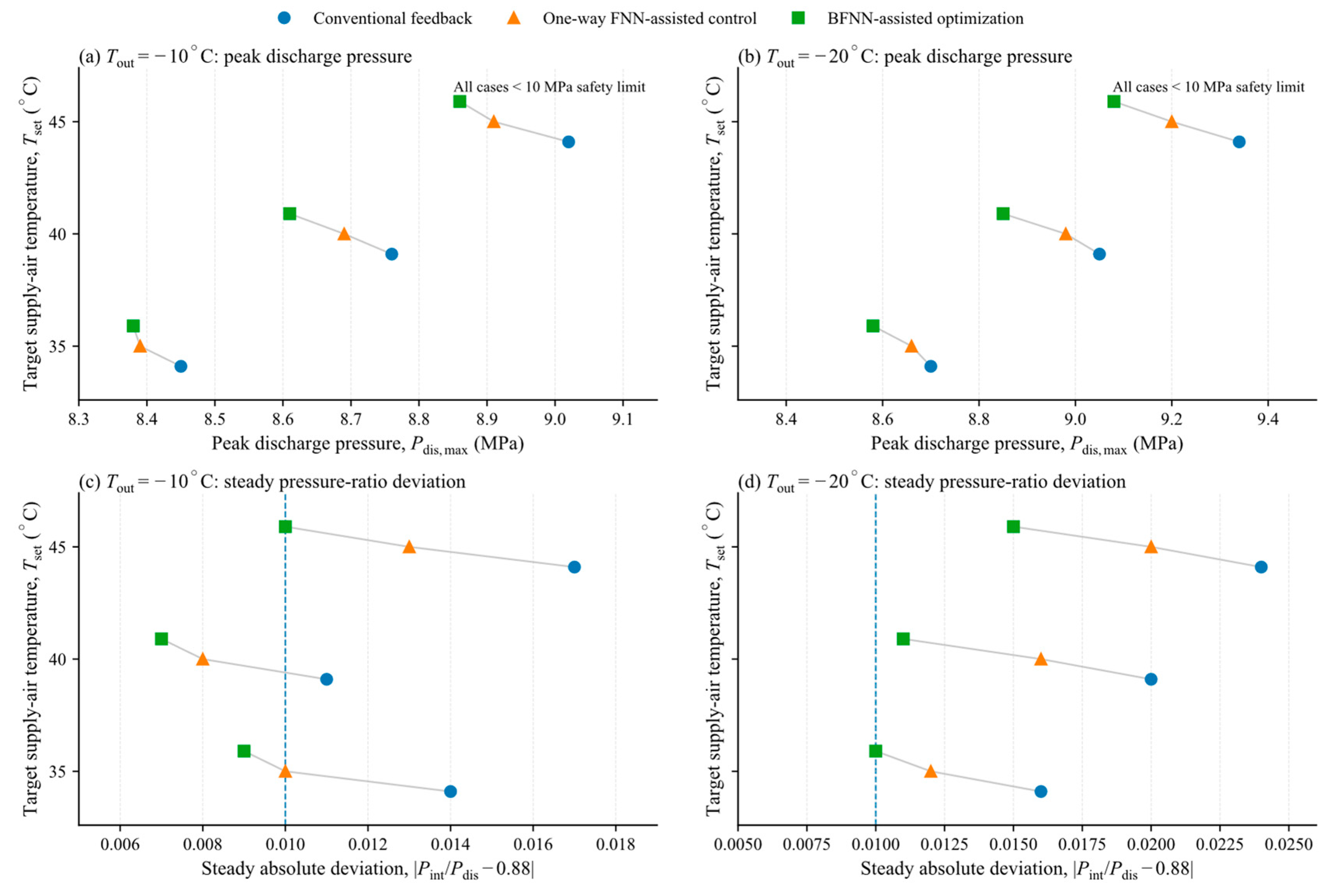
Figure 8 compares the peak discharge pressures and steady-state pressure-ratio deviations of the three strategies to examine the discharge-pressure peaks and intermediate-pressure matching during rapid regulation. The connecting lines are used only to compare the strategies under the same ambient temperature and supply-air temperature target; they do not represent continuous changes between the strategies.

Figure 8a,b show that the peak discharge pressure generally increased as the target supply-air temperature rose from 35 to 45 °C. Across the six operating conditions, the peak discharge pressure of the BFNN-assisted strategy ranged from 8.38 to 9.08 MPa, lower than the 8.39–9.20 MPa range of the unidirectional FNN-assisted strategy and the 8.45–9.34 MPa range of the rule-based feedback strategy. The corresponding mean values for the BFNN-assisted, unidirectional FNN-assisted, and rule-based feedback strategies were 8.73, 8.81, and 8.89 MPa, respectively, all below the safety limit of 10 MPa.

As shown in Figure 8c,d, relative to the pressure-coordination reference ratio P_int/P_dis = 0.88, the absolute pressure-ratio deviation of the BFNN-assisted strategy ranged from 0.007 to 0.015, lower than the ranges of 0.008–0.020 for the unidirectional FNN-assisted strategy and 0.011–0.024 for the rule-based feedback strategy. The corresponding mean values were 0.0103, 0.0132, and 0.0170, respectively. The BFNN-assisted strategy reduced the mean absolute pressure-ratio deviation by 21.5% and 39.2% compared with the unidirectional FNN-assisted and rule-based feedback strategies, respectively. At an ambient temperature of −10 °C and a target supply-air temperature of 40 °C, the deviation was lower than those under the adjacent operating conditions. This indicates that the coordination performance is also influenced by the operating-parameter combination and operating-condition range, rather than varying strictly monotonically with the heating load.

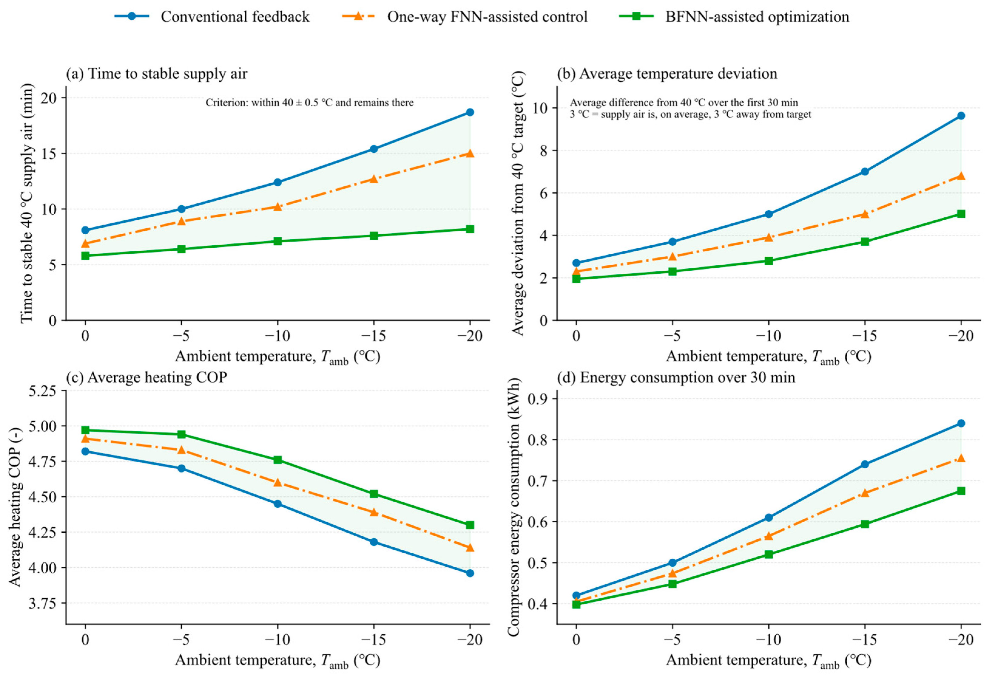
5.4. Regulation Performance and Energy Efficiency at Different Ambient Temperatures

Start-up tests were conducted at ambient temperatures of 0, −5, −10, −15, and −20 °C under a supply-air temperature target of 40 °C, a cabin-side airflow rate of 300 m³/h, and 100% fresh-air conditions. The stabilization time, mean absolute supply-air temperature deviation during the first 30 min after start-up, time-averaged heating COP, and compressor energy consumption were evaluated, as shown in Figure 9. The 30 min mean absolute supply-air temperature deviation was used to quantify the overall temperature deviation during start-up, complementing the settling time by accounting for the magnitude of the temperature error before stabilization. The instantaneous heating COP was calculated as the ratio of heating capacity to compressor power at each sampling instant, and the reported COP was obtained by averaging these instantaneous values over the 30 min test period. In contrast, compressor energy consumption was obtained by integrating compressor power over the same period. As the ambient temperature decreased, both the stabilization time and the mean absolute supply-air temperature deviation increased. The BFNN-assisted strategy yielded lower values for both metrics at all ambient temperatures, with a more pronounced advantage under lower-temperature conditions.

Figure 9c,d show that, as the ambient temperature decreased, the heat-transfer capacity of the outdoor heat exchanger weakened, while the compression ratio and compressor power increased. Consequently, the 30 min time-averaged heating COP decreased and the compressor energy consumption increased. The BFNN-assisted strategy achieved a higher COP and lower energy consumption at all ambient temperatures. This indicates that its faster recovery did not rely on an excessive increase in compressor power, but resulted from the system reaching a suitable combination of operating parameters more quickly.

At −20 °C, the stabilization times of the BFNN-assisted, unidirectional FNN-assisted, and rule-based feedback strategies were approximately 8.2, 15.0, and 18.7 min, respectively. Their mean absolute temperature differences over the first 30 min were approximately 5.0, 6.8, and 9.6 °C; the time-averaged heating COP values were approximately 4.30, 4.15, and 3.95; and the compressor energy consumptions were approximately 0.68, 0.75, and 0.84 kWh, respectively. Compared with the conventional rule-based feedback strategy, the BFNN-assisted strategy reduced the stabilization time by 56.3%, decreased the mean absolute temperature difference by 47.9%, increased the time-averaged heating COP by 8.9%, and reduced energy consumption by 19.0%. It should be noted that the reported COP is the time average of the instantaneous heating-capacity-to-compressor-power ratio, whereas compressor energy consumption is obtained from the time integral of compressor power. Therefore, cumulative compressor energy consumption is not the denominator of the reported time-averaged COP, and the relative changes in the two metrics are not required to be proportional. The larger reduction in cumulative energy consumption is consistent with the shorter transient adjustment period and the lower compressor-power demand observed under BFNN-assisted control. The three repeated tests showed consistent trends for all three control strategies. Across the repeated tests, the standard deviations of the stabilization time, time-averaged heating COP, and compressor energy consumption were within 0.2–0.4 min, 0.05–0.08, and 0.02–0.03 kWh, respectively, indicating good experimental repeatability.

5.5. Dynamic Recovery and Energy-Efficiency Performance Under a Cabin-Side Airflow Step Disturbance

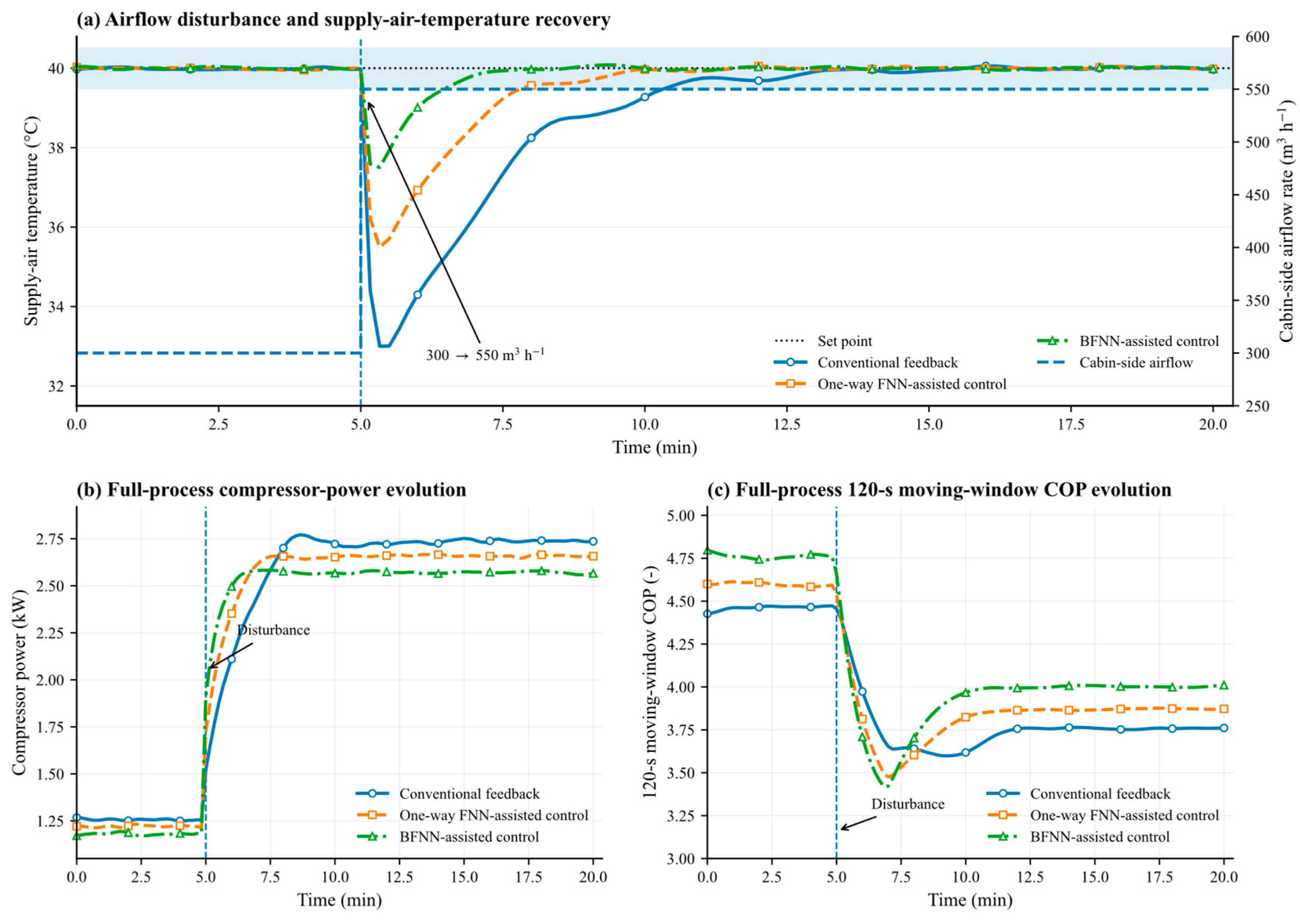
A cabin-side airflow step test was conducted under 100% fresh-air conditions, an ambient temperature of −10 °C, and a supply-air temperature target of 40 °C. The system was first stabilized at a cabin-side airflow rate of 300 m³/h. At 5 min, the airflow rate was increased to 550 m³/h. The test lasted 20 min, with a sampling interval of 10 s. Figure 10 presents the supply-air temperature, compressor power, and heating COP. The COP is calculated using a 120 s moving window. It is defined as the ratio of cumulative heating output to cumulative compressor electricity consumption, which reduces pointwise fluctuations caused by asynchronous transient responses.

As shown in Figure 10a, the supply-air temperature decreased briefly for all three strategies after the airflow rate increased. The minimum supply-air temperatures under the BFNN-assisted, unidirectional FNN-assisted, and conventional rule-based feedback strategies were approximately 37.50, 35.49, and 33.00 °C, respectively, corresponding to maximum temperature drops of 2.50, 4.51, and 7.09 °C. The recovery times to reach and remain within 40 ± 0.50 °C were 1.67, 3.00, and 5.50 min, respectively. Compared with rule-based feedback, the BFNN-assisted strategy shortened the recovery time by 69.7%, demonstrating better supply-air temperature recovery after the airflow step disturbance.

For the three repeated airflow step tests, the standard deviations of the maximum supply-air temperature drop and recovery time were within 0.1–0.3 °C and 0.1–0.3 min, respectively, confirming good repeatability of the observed disturbance-recovery behavior. Figure 10b shows that all three strategies increased the compressor power after the airflow step. The peak compressor powers of the BFNN-assisted, unidirectional FNN-assisted, and conventional rule-based feedback strategies were approximately 2.59, 2.68, and 2.81 kW, respectively, while their subsequent steady-state powers were approximately 2.57, 2.66, and 2.74 kW. The BFNN-assisted strategy responded faster and exhibited less overshoot. Its rapid temperature recovery did not rely on a sustained increase in compressor power, indicating that the compressor speed and throttling parameters were adjusted more quickly to the new operating state.

As shown in Figure 10c, the 120 s moving-window COP values of all three strategies transitioned smoothly to their new steady states after the disturbance. The steady-state COP values of the BFNN-assisted, unidirectional FNN-assisted, and rule-based feedback strategies were approximately 4.00, 3.87, and 3.76, respectively. The BFNN-assisted strategy increased the COP by 3.4% and 6.5% compared with the unidirectional FNN-assisted and rule-based feedback strategies, respectively. At approximately the same air-side heating output, the BFNN-assisted strategy maintained lower steady-state compressor power and higher heating energy efficiency.

5.6. Ablation Analysis of the BFNN-Assisted Control Framework

To separately evaluate the contributions of inverse initialization and the shared-parameter architecture, an ablation experiment was conducted under the representative −20 °C cold-start condition (Table 4). Three configurations were compared: the original one-way FNN-assisted Strategy B, an ablated bidirectional configuration using independently trained forward and inverse FNNs, and the complete shared-parameter BFNN-assisted Strategy C. All candidate-search settings, operating constraints, feedback-correction rules, and safety-protection settings were kept identical. Therefore, the comparison between the one-way FNN and the independently trained bidirectional FNN isolates the contribution of inverse initialization, while the comparison between the independently trained bidirectional FNN and the complete BFNN reflects the additional contribution of the shared-parameter architecture.

Table 4. Ablation analysis of the BFNN-assisted control framework under the −20 °C cold-start condition.

Configuration	Initialization	Forward Evaluation	Stabilization Time/Min	No. of Adjustments	Mean Absolute Temperature Deviation
One-way FNN	Previous-cycle setpoints	Independent forward FNN	15.0	8	6.8 °C
Independent bidirectional FNN	Independent inverse FNN	Independent forward FNN	10.8	6	5.7 °C
Shared-parameter BFNN	Shared inverse path	Shared forward path	8.2	5	5.0 °C

Table 4. Ablation analysis of the BFNN-assisted control framework under the −20 °C cold-start condition.

Configuration	Initialization	Forward Evaluation	Stabilization Time/Min	No. of Adjustments	Mean Absolute Temperature Deviation
One-way FNN	Previous-cycle setpoints	Independent forward FNN	15.0	8	6.8 °C
Independent bidirectional FNN	Independent inverse FNN	Independent forward FNN	10.8	6	5.7 °C
Shared-parameter BFNN	Shared inverse path	Shared forward path	8.2	5	5.0 °C

Compared with the one-way FNN-assisted configuration, introducing the independent inverse FNN reduced the stabilization time from 15.0 to 10.8 min, the number of control adjustments from 8 to 6, and the 30 min mean absolute supply-air temperature deviation from 6.8 to 5.7 °C. This indicates that inverse initialization can substantially narrow the initial search range and reduce repeated parameter adjustments. When the independently trained forward and inverse networks were further replaced by the shared-parameter BFNN, the stabilization time decreased to 8.2 min, the number of adjustments was further reduced to 5, and the mean absolute temperature deviation decreased to 5.0 °C. These results suggest that the shared-parameter architecture provides an additional improvement beyond inverse initialization by enabling the forward and inverse tasks to reuse common thermodynamic coupling features.

6. Discussion

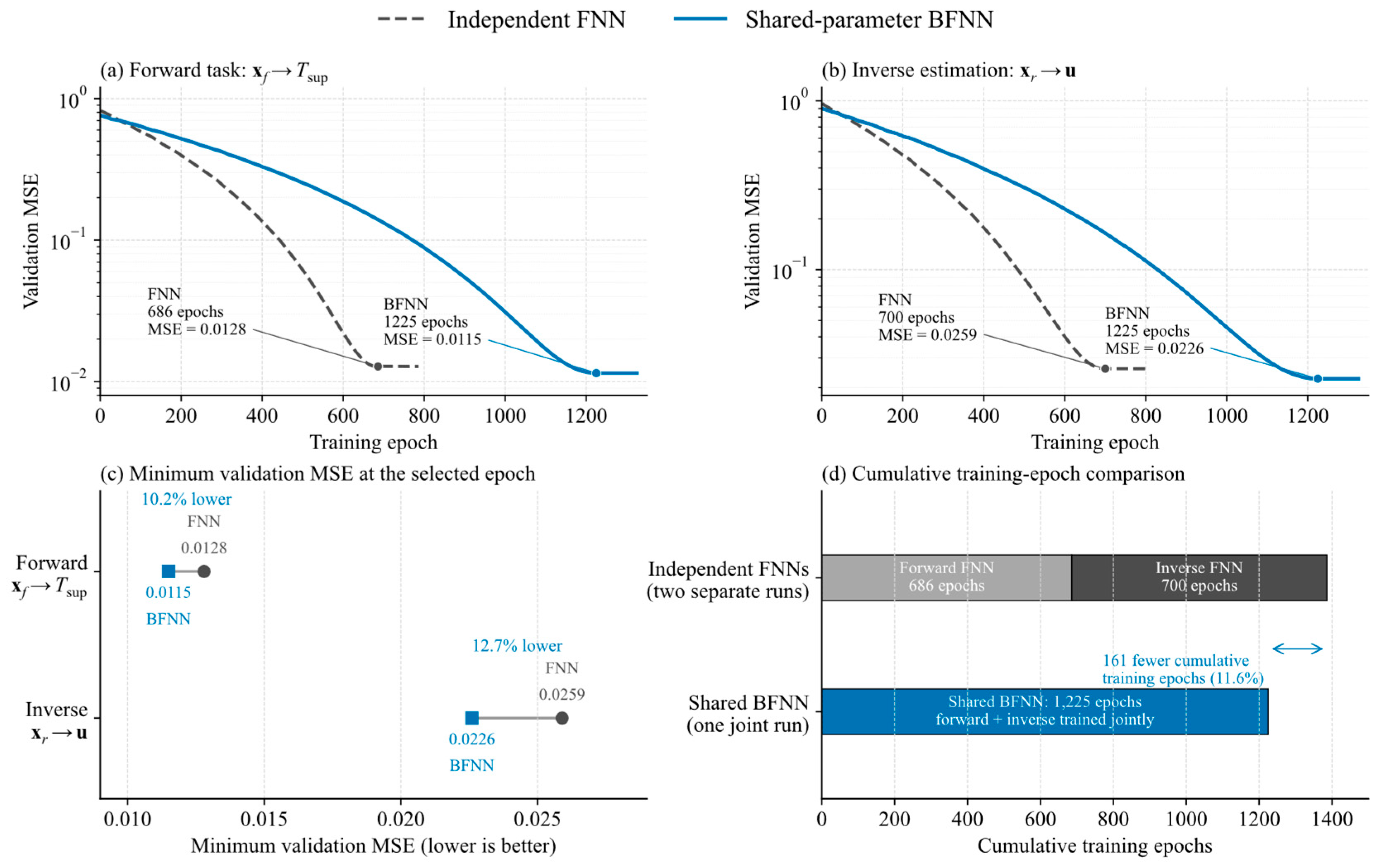
The shared-parameter BFNN achieved test-set R² values of 0.985 for supply-air temperature and 0.967 for compressor speed. The supply-air temperature RMSE decreased from 0.470 °C for the independent FNN to 0.381 °C for the BFNN under the same dataset partition and repeated-training protocol (Table 2). For comparison, Evens and Arteconi [24] developed a water/water heat pump digital twin using feedforward and long short-term memory networks. Their best history-based model maintained electrical-power prediction errors within ±10% for 79.70% of the evaluated time during multiple-step prediction. These metrics cannot be directly ranked against the present temperature-prediction errors because the predicted quantities, prediction horizons, and system configurations differ. The methodological distinction is that the present BFNN jointly provides quasi-steady-state forward estimates and target-conditioned inverse estimates, whereas the digital twin approach incorporates operating history to predict subsequent system behavior. The present accuracy results therefore support improvement over the independent FNN baseline within the investigated dataset, without establishing superiority over dynamic prediction models.

In terms of dynamic regulation, Miao et al. [20] experimentally evaluated a data-driven model predictive controller for a transcritical CO₂ thermal system. Their controller predicts system behavior over a finite horizon and determines control inputs using the predicted response. The present framework instead uses inverse estimation to initialize a bounded local search and forward prediction to evaluate candidate quasi-steady-state operating points, with transient deviations corrected through measured feedback. Under the −20 °C cold-start condition, the BFNN-assisted, one-way FNN-assisted, and rule-based feedback strategies achieved stabilization times of 8.2, 15.0, and 18.7 min, respectively. The ablation results further show that inverse initialization reduced the stabilization time from 15.0 to 10.8 min, while the shared-parameter architecture provided an additional reduction to 8.2 min. These results identify contributions within the proposed framework, but do not establish a response-speed advantage over model predictive control, which was not evaluated on the same experimental platform.

Energy-performance comparisons also require consideration of the control objective and system boundary. Wang et al. [21] developed an integrated model predictive control strategy to minimize total thermal-management-system power while maintaining the required cabin and battery temperatures, reporting simulated energy savings of 5.9–10.3% relative to PI control. Miao et al. [20] optimized the system COP while maintaining the required cooling or heating capacity. In the present study, Equation (9) penalizes supply-air temperature error and operating-parameter changes rather than directly optimizing COP or power. Nevertheless, the −20 °C cold-start test showed an 8.9% increase in time-averaged heating COP and a 19.0% reduction in compressor energy consumption relative to rule-based feedback. These benefits accompanied faster temperature regulation, but their magnitudes should not be directly ranked against the published savings because the energy-accounting boundaries, operating conditions, evaluation periods, and baseline controllers differ. The proposed method should therefore be regarded as a temperature-regulation strategy with demonstrated energy benefits under the tested conditions, rather than as a generally energy-optimal controller.

Several limitations should be considered when interpreting the present results. First, the BFNN predicts quasi-steady-state supply-air temperature and does not explicitly describe thermal inertia or full transient system dynamics. The reported dynamic improvement therefore reflects the integrated effect of candidate generation, forward evaluation, and measured-feedback correction. Second, the experiments were conducted on a single secondary-throttling CO₂ heat pump platform within the investigated ambient-temperature and airflow ranges under 100% fresh-air conditions. The generalization of the model to other system configurations, recirculation ratios, wider ambient conditions, and long-term vehicle operation therefore requires further validation. Future work will extend the training dataset to broader operating ranges, investigate online model adaptation, and evaluate the method under more realistic vehicle-driving and cabin-load conditions.

7. Conclusions

To address the strengthened multi-component coupling, difficulty in coordinating operating parameters, and delayed supply-air temperature response during the low-temperature heating of electric-vehicle CO₂ heat pumps, this study proposes a shared-parameter BFNN-based prediction-assisted control method. Unlike approaches that model forward and inverse prediction separately, the proposed method uses a single model. It jointly learns the forward and inverse mappings among air-side operating conditions, operating parameters, and supply-air temperature. It also reuses thermodynamic coupling features shared by both tasks through shared hidden layers. To address the multiple-solution nature of the inverse mapping, the inverse path generates only candidate operating parameters. These candidates are then corrected through forward supply-air temperature evaluation, operating-range constraints, and measured feedback, forming a prediction-assisted regulation process of “inverse generation–forward evaluation–constraint and feedback correction.” The main conclusions are as follows:

(1) Across five independent training runs, the shared-parameter BFNN achieved lower validation errors than the independent FNNs. The mean minimum validation MSEs for the forward and inverse tasks were reduced by approximately 10.0% and 12.6%, respectively. On the test set, the prediction R² values for supply-air temperature, compressor speed, EEV1 opening, and EEV2 opening were 0.985, 0.967, 0.911, and 0.933, respectively.

(2) The BFNN-assisted strategy exhibited faster supply-air temperature response and recovery under both low-temperature cold-start and airflow-disturbance conditions. During a cold start at an ambient temperature of −20 °C, the supply-air temperature stabilization time was 8.2 min, representing reductions of 45.6% and 56.3% compared with the unidirectional FNN-assisted and rule-based feedback strategies, respectively. At an ambient temperature of −10 °C, when the cabin-side airflow rate was stepped from 300 to 550 m³/h, the BFNN-assisted strategy limited the maximum supply-air temperature drop to 2.50 °C and achieved a recovery time of 1.67 min.

(3) Under an ambient temperature of −20 °C, a target supply-air temperature of 40 °C, and a test duration of 30 min, the BFNN-assisted strategy reduced the mean absolute temperature difference by 47.9%. It also increased the time-averaged heating COP by 8.9% and reduced compressor energy consumption by 19.0% compared with conventional rule-based feedback.

The present study is limited to a single experimental platform and the investigated operating range, while the BFNN represents quasi-steady-state behavior rather than full transient dynamics. Further work will focus on broader operating conditions, model adaptation, and validation under more realistic vehicle operating scenarios.