Transformer-Based Solar Irradiance Forecasting Model for Coastal and Microclimate-Sensitive Areas of First District of Batangas

Abstract

Accurate solar irradiance forecasting is a key prerequisite for reliable solar photovoltaic (PV) operation, effective energy management, and system optimization. Conventional forecasting methods, such as historical averaging, persistence models, and coarse-resolution numerical weather prediction outputs, often exhibit limited performance in coastal and microclimate-sensitive environments where irradiance is characterized by rapid and nonlinear atmospheric variability. Batangas District 1, a coastal and peninsular region in the Philippines, is particularly influenced by sea–land breeze circulation, convective cloud development, humidity fluctuations, and aerosol transport, resulting in highly non-stationary irradiance patterns and persistent forecasting errors. Although recent advances in deep learning, particularly Transformer-based architectures, have demonstrated strong potential for modeling complex atmospheric time-series, locally developed and validated models for Philippine coastal environments remain scarce. Moreover, this study addresses this gap by developing FAT-Former, a Transformer-based solar irradiance forecasting algorithm designed to capture the microclimatic characteristics of Batangas District 1. The proposed model substantially outperformed the persistence benchmark and demonstrated strong temporal representation capability, achieving the lowest mean peak-time error and preserving 101.30% of the observed variance. However, predictive performance deteriorated under precipitation events and highly variable daylight conditions, while the resulting prediction intervals exhibited under-calibration. These findings suggest that forecasting performance in coastal environments depends not only on model complexity but also on the model’s ability to adapt to rapidly changing atmospheric regimes. All in all, FAT-Former demonstrates the potential of Transformer-based architectures for localized and uncertainty-aware solar irradiance forecasting. Further evaluation across diverse coastal and microclimate-sensitive locations is recommended to assess the model’s robustness, transferability, and broader generalizability.

1. Introduction

Accurate solar irradiance forecasting is essential for the reliable operation, planning, and optimization of solar photovoltaic (PV) systems. Conventional forecasting approaches typically rely on historical averages, persistence models, or coarse-resolution numerical weather prediction (NWP) outputs. Although these methods can perform adequately in geographically homogeneous and inland environments, their accuracy often declines in coastal and microclimate-sensitive regions because of their limited ability to capture rapid, nonlinear atmospheric variability. Batangas District 1, a coastal and peninsular region of the Philippines, experiences complex microclimatic conditions in which solar irradiance is strongly influenced by sea–land breeze circulation, rapid convective cloud development, humidity fluctuations, and aerosol transport. These interacting atmospheric processes generate high-frequency, nonlinear, and non-stationary irradiance patterns that remain challenging for traditional forecasting models to represent accurately [1,2,3]. Consequently, deterministic and climatology-based forecasting approaches may exhibit systematic biases and substantial short-term prediction errors when applied to solar PV operations in coastal environments.

In parallel, the integration of advanced deep learning architectures, particularly Long Short-Term Memory (LSTM) networks and Transformer models, represents a significant advancement in improving the accuracy and reliability of complex environmental forecasting and microclimatic analysis [4]. LSTM networks are widely recognized for their ability to model sequential dependencies and mitigate the vanishing gradient problem commonly encountered in conventional recurrent neural networks. However, their recurrent structure requires observations to be processed sequentially, which can constrain computational efficiency and make the representation of long-range temporal dependencies more difficult as the temporal distance between observations increases. These limitations become more pronounced in highly dynamic coastal environments, where localized atmospheric variability, rapid weather transitions, and nonlinear interactions among meteorological factors can significantly influence solar irradiance patterns [5].

Transformer-based architectures provide an alternative mechanism for addressing these limitations through self-attention, which enables the model to directly evaluate relationships among different time steps within the historical input sequence. Multi-head attention further allows the simultaneous extraction of multiple temporal and meteorological relationships, enabling the model to capture complex dependencies occurring across different temporal scales. In addition, positional encoding preserves the chronological order of observations despite the absence of recurrent processing. Unlike LSTM-based architectures, Transformer computations across the input sequence can be performed largely in parallel, thereby improving computational efficiency during training while facilitating the modeling of long-range temporal relationships. Consequently, these characteristics make Transformer architectures particularly suitable for solar irradiance forecasting, where abrupt fluctuations and nonlinear dependencies among irradiance and meteorological variables may occur over multiple temporal scales.

Nonetheless, recent developments have further explored hybrid and integrated frameworks that combine the temporal modeling capabilities of LSTM networks with the parallel processing and long-range dependency modeling offered by Transformer architectures [6]. When supplemented by complementary techniques such as convolutional neural networks (CNNs) and remote-sensing-derived meteorological data, these frameworks can provide more robust representations of nonlinear climatic interactions and spatiotemporal dependencies. Furthermore, the incorporation of probabilistic forecasting approaches and frequency-domain analysis extends these models beyond purely deterministic prediction by enabling the quantification of forecasting uncertainty. Such uncertainty-aware predictions are particularly valuable in coastal environments, where rapidly changing atmospheric conditions can introduce substantial variability into solar irradiance patterns [5].

2. Literature Review

Solar irradiance forecasting is a foundational requirement for efficient solar photovoltaic (PV) system planning and grid integration. Traditional forecasting approaches—such as persistence models, empirical regression, and numerical weather prediction (NWP) have been widely used due to their interpretability and low computational cost. However, these models assume relatively stable atmospheric behavior and smooth temporal variation, making them less effective in environments with strong local meteorological dynamics [1,7].

Recent studies have emphasized that coastal and tropical regions exhibit significantly higher solar irradiance variability than inland areas. This variability is largely driven by sea–land breeze circulation, rapid cloud evolution, moisture convergence, and aerosol transport, all of which introduce abrupt and nonlinear fluctuations in surface solar radiation. Xu et al. demonstrated that sea–land breeze mechanisms directly influence short-term coastal irradiance patterns, leading to forecast errors when using climatology-based or coarse-resolution models. Similar findings were reported by [8], which showed that local/shelf/global models can underperform nearshore and that ML approaches can outperform generic global models in coastal settings.

To overcome the limitations of conventional forecasting approaches, recent research has increasingly shifted toward machine learning (ML) methods, including artificial neural networks (ANNs), support vector regression (SVR), and ensemble learning architectures, which have demonstrated superior predictive performance over classical statistical and persistence-based benchmarks for solar irradiance forecasting [9]. Unlike conventional models that depend heavily on predefined statistical assumptions, ML approaches learn complex and nonlinear relationships directly from historical observations, enabling them to capture higher-order interactions among meteorological variables such as irradiance, cloud characteristics, relative humidity, air temperature, and wind speed. This data-driven learning capability is particularly advantageous in coastal environments, where localized atmospheric processes and intermittent cloud dynamics can produce abrupt irradiance fluctuations that are difficult to characterize using fixed or simplified model structures. Moreover, hybrid and ensemble frameworks that integrate ANNs or SVRs with tree-based learners, as well as ML models coupled with numerical weather prediction (NWP) outputs, have demonstrated improved robustness across forecast horizons and contrasting weather regimes by reducing prediction bias, variance, and model-specific weaknesses [10]. These developments indicate a broader transition from static forecasting schemes toward adaptive, data-driven frameworks capable of responding to changing atmospheric conditions. Accordingly, state-of-the-art solar irradiance forecasting increasingly emphasizes informed feature selection and engineering, weather-regime characterization, model adaptation, and post-processing to improve not only point-forecast accuracy but also the reliability of predictions for grid integration, PV power management, and energy-yield estimation [9].

Recurrent neural network (RNN) architectures, including long short-term memory (LSTM) and gated recurrent unit (GRU) networks, have further advanced short-term solar irradiance forecasting by capturing temporal dependencies in meteorological time-series. However, despite their success in modeling sequential patterns, multiple studies note that RNN-based models can still exhibit limitations related to vanishing/exploding gradients, restricted long-term memory retention, and sensitivity to high-frequency noise under rapidly changing sky conditions—factors that can reduce predictive performance in highly variable environments [11,12].

More recently, Transformer-based architectures have emerged as a powerful alternative for solar irradiance forecasting. These models rely on self-attention mechanisms that enable explicit modeling of long-range temporal dependencies and dynamic feature relevance. Several studies report that Transformer and attention-based models outperform LSTM and CNN-based architectures in both short-term and ultra-short-term solar forecasting tasks, particularly in highly variable weather conditions [13]. Vision-based Transformer models using sky images and multimodal data have also demonstrated strong performance in nowcasting applications by effectively capturing cloud motion and evolution.

Hybrid forecasting frameworks that combine numerical weather prediction (NWP) information with deep learning models can leverage both atmospheric-model outputs and data-driven learning to improve renewable energy forecasting. In a related energy management context, Ghafoori demonstrated the effectiveness of integrating machine learning-based forecasting with downstream optimization, using DNN and LSTM models to predict building electricity demand and subsequently optimize EV charging and discharging schedules [14]. This broader hybrid forecasting–optimization paradigm supports the integration of physically informed weather variables with advanced learning architectures for short-term photovoltaic forecasting [14,15]. Similarly, multimodal approaches that fuse satellite imagery and ground-based meteorological measurements improve both accuracy and robustness in solar radiation prediction by capturing cloud features and surface effects more effectively [16].

Despite these advances, most existing studies focus on generalized datasets or regions outside Southeast Asia, with limited localization to Philippine coastal microclimates. A clear research gap therefore remains in developing Transformer-based solar irradiance forecasting algorithms specifically tailored to coastal districts such as Batangas District 1. Addressing this gap is essential to determine whether advanced deep-learning models can effectively capture localized irradiance variability and improve forecasting reliability under rapidly changing coastal weather conditions. Such localized forecasting capability can reduce operational uncertainty and support more reliable large-scale solar energy integration in coastal regions. Future research should focus on cross-location validation, adaptation to diverse weather regimes, and uncertainty calibration to establish the robustness and broader applicability of these models.

3. Methodology

3.1. Research Framework

This study adopts a quantitative, model-driven time-series forecasting framework for the development and evaluation of the Feature-Augmented Transformer (FAT-Former) for one-hour-ahead solar irradiance forecasting. The framework is intended to support forecasting applications in coastal and microclimate-sensitive environments, where solar irradiance may exhibit substantial short-term variability associated with changing atmospheric conditions.

Moreover, the methodological contribution of FAT-Former lies not in the introduction of a new attention mechanism, but in the integration of complementary feature-engineering and representation-learning components within an encoder-only Transformer forecasting framework. Specifically, FAT-Former combines causal time-domain features, frequency-domain information, Principal Component Analysis (PCA), Mutual Information (MI)-based feature relevance analysis, training-only standardization, Transformer-based temporal representation learning, and conditional quantile regression.

Furthermore, this investigation is deliberately confined to a single geographic location. Accordingly, FAT-Former is evaluated as a location-specific forecasting framework rather than as a spatial forecasting model spanning multiple coastal sites. Nevertheless, the proposed methodology is designed as a transferable framework that can subsequently be validated across systematically characterized coastal and microclimate-sensitive locations to assess its robustness and broader generalizability.

3.2. Data Sources and Description

The meteorological and solar radiation variables analyzed in this study were obtained from the NASA/POWER CERES/MERRA2 hourly dataset at its native spatial and temporal resolution, provided by the NASA Langley Research Center Atmospheric Science Data Center (ASDC) (2024). This comprehensive dataset spans a significant period, from 1 January 2015, to 22 October 2024, providing nearly a decade of hourly observations [17,18]. The data correspond to a specific geographical location identified by Latitude 13.9955° and Longitude 121.0165°, with an average elevation of 162.3 m for the $0.5\times 0.625$ degree latitude/longitude region, as determined by MERRA-2.

Furthermore, the dataset includes several critical parameters essential for environmental and energy-related analyses. Solar radiation components, derived from CERES SYN1deg, include “All Sky Surface Shortwave Downward Direct Normal Irradiance (Wh/m²),” “All Sky Surface Shortwave Diffuse Irradiance (Wh/m²),” “All Sky Surface UVA Irradiance (W/m²),” and “All Sky Surface UVB Irradiance (W/m²).” Additionally, atmospheric conditions are covered by MERRA-2 parameters such as “Temperature at 2 Meters (°C),” “Precipitation Corrected (mm/h),” and “Surface Pressure (kPa)”.

A standardized approach is employed for handling missing data points, where a value of $-999$ indicates instances in which data could not be computed or fell outside the availability range of the sources. This convention ensures clarity and facilitates proper data handling during analysis, preventing misinterpretation of unrecorded values. This robust dataset is therefore well-suited for detailed investigations into localized climate patterns and renewable energy potential.

3.3. Data Processing, Time Alignment and Chronological Partitioning

All timestamp fields were converted to Coordinated Universal Time (UTC), indexed chronologically, and merged according to exact timestamp correspondence. Duplicate timestamps were removed, and the resulting observations were arranged in chronological order. The temporal resolution was verified to ensure that consecutive observations corresponded to one-hour intervals.

The forecasting problem was formulated as a 24 h-look-back, one-hour-ahead prediction task. Thus, all information available up to forecast origin $t$ was used to estimate solar irradiance at time $t+1$.

To preserve temporal causality, the dataset was divided chronologically rather than randomly. Eligible forecast origins were partitioned as follows:

$$\begin{gathered} 70\%training\left(\mathrm{55,204}\right):1\mathrm{J}\mathrm{a}\mathrm{n}\mathrm{u}\mathrm{a}\mathrm{r}\mathrm{y}2015to20\mathrm{A}\mathrm{p}\mathrm{r}\mathrm{i}\mathrm{l}2021, \\ 15\%validation\left(\mathrm{11,829}\right):20\mathrm{A}\mathrm{p}\mathrm{r}\mathrm{i}\mathrm{l}2021to26\mathrm{A}\mathrm{u}\mathrm{g}\mathrm{u}\mathrm{s}\mathrm{t}2022, \\ 15\%independenttesting\left(\mathrm{11,830}\right):26\mathrm{A}\mathrm{u}\mathrm{g}\mathrm{u}\mathrm{s}\mathrm{t}2022to31\mathrm{D}\mathrm{e}\mathrm{c}\mathrm{e}\mathrm{m}\mathrm{b}\mathrm{e}\mathrm{r}2023. \end{gathered}$$

The training partition was used to estimate preprocessing parameters and optimize model weights. The validation partition was used exclusively for model development, learning-rate adjustment, and early stopping. The final 15% chronological partition remained independent and was used only for the final performance evaluation.

Additionally, the chronological partition was defined before PCA, Mutual Information analysis, imputation, standardization, and model training. Consequently, no information from the validation or independent test periods was used to estimate preprocessing parameters.

3.4. Feature Augmented Transformer (FAT) Pipeline

The proposed FAT-Former framework is a hybrid time-series forecasting architecture that integrates feature engineering, feature selection, Transformer-based sequence learning, and probabilistic forecasting into a unified pipeline. The framework is designed to improve predictive accuracy and uncertainty estimation by combining temporal feature extraction, mutual information-based feature relevance analysis, positional encoding, and attention-driven representation learning.

3.4.1. Time Domain Feature

To explicitly encode short-term temporal behavior, statistical features were calculated from the observed target series using only information available at or before forecast origin $t$.

A rolling window of 24-hourly observations was used to represent the most recent diurnal cycle.

The 24 h rolling mean was calculated as

$${\mu }_t^{\left(24\right)}=\frac{1}{24}\sum _{i=0}^{23}{y}_{t-i},$$

(1)

where $y_t$ represents the observed solar irradiance at time $t$. The rolling mean provides information regarding the recent irradiance level and local temporal trend.

The corresponding rolling standard deviation was calculated as

$${\sigma }_t^{\left(24\right)}=\sqrt{{\displaystyle \frac{1}{23}}\sum _{i=0}^{23}{\left(y_{t-i}-{\mu }_t^{\left(24\right)}\right)}^2}$$

(2)

which quantifies the degree of short-term variability within the preceding 24 h period.

To represent immediate temporal change, the first-order difference was computed as

$$\Delta y_t=y_t-y_{t-1}.$$

(3)

This feature increases sensitivity to abrupt changes between consecutive hourly observations.

A 24 h seasonal difference was additionally calculated as

$${\Delta }_{24}{y}_t=y_t-y_{t-24},$$

(4)

allowing the model to represent deviations from the irradiance observed at the corresponding hour of the preceding day.

All rolling and differenced features were constructed causally. No centered rolling windows or future observations were included.

3.4.2. Frequency-Domain Features

In addition to time-domain statistics, spectral information was extracted to represent periodic and oscillatory characteristics of the irradiance signal.

For each causal 24 h historical window, the discrete Fourier transform was computed as

$$X_k=\sum _{n=0}^{N-1}{y}_n{e}^{-j2\pi kn/N},N=24,$$

(5)

and spectral energy was subsequently calculated from the Fourier coefficients:

$$E_t=\sum _k{\mid X_k\mid }^2.$$

(6)

This feature provides a compact representation of periodic information that rolling statistics or differenced values may not explicitly capture.

3.4.3. Auxiliary Feature Compression

The auxiliary meteorological variables were compressed using Principal Component Analysis (PCA) to reduce redundancy among correlated environmental variables.

Prior to PCA, missing auxiliary observations were imputed using parameters estimated from the training partition. The auxiliary variables were then standardized to zero mean and unit variance. Both the imputer and scaler were fitted exclusively on the training data and subsequently applied unchanged to the validation and test partitions.

For a standardized auxiliary feature vector $a_t$, PCA is expressed as

$$p_t=W_{PCA}^T{a}_t,$$

(7)

where $W_{PCA}$ contains the principal-component loading vectors.

The first five principal components were retained:

$$p_t={\left[p_{t,5}\right]}^T.$$

These five components preserved approximately 78% of the variance represented by the standardized auxiliary meteorological variables in the experimental implementation.

3.4.4. Mutual Information-Based Feature Relevance Selection

Mutual Information regression was employed to quantify the statistical dependence between each candidate predictor $X_j$ and the corresponding one-hour-ahead target $Y$. Unlike conventional linear correlation, MI can represent nonlinear as well as linear relationships.

For predictor $X_j$ and target $Y$, Mutual Information is defined as

$$I\left(Y\right)=\int \int p\left(y\right)loglog\left[{\displaystyle \frac{p\left(y\right)}{p\left(x_j\right)p\left(y\right)}}\right]d{x}_j\hspace{0.17em}dy.$$

(8)

The resulting MI values were normalized to the interval $\left[1\right]$:

$$I_j^{\left(norm\right)}={\displaystyle \frac{I_j-I_{min}}{I_{max}-I_{min}}}.$$

(9)

The candidate predictor set comprised five engineered temporal and spectral features and five PCA components. All ten predictors were systematically ranked using normalized mutual information (MI) scores.

The experimental configuration specifies

$$K=10.$$

Because the current candidate set also contains ten predictors, all candidate variables are retained. Accordingly, in the present implementation, MI functions primarily as a feature-relevance ranking mechanism rather than a dimensionality-reduction procedure.

3.4.5. Scaling and Sequence Construction

Following feature ranking, the retained predictors were standardized using z-score normalization. For feature $j$ at time $t$,

$$x_{t,j}^{\prime }={\displaystyle \frac{x_{t,j}-{\mu }_j^{\left(train\right)}}{{\sigma }_j^{\left(train\right)}}},$$

(10)

where ${\mu }_j^{\left(train\right)}$ and ${\sigma }_j^{\left(train\right)}$ denote the mean and standard deviation of feature $j$, respectively, estimated exclusively from the training dataset.

The target solar irradiance variable was standardized independently from the predictor variables:

$$y_t^{\prime }={\displaystyle \frac{y_t-{\mu }_y^{\left(train\right)}}{{\sigma }_y^{\left(train\right)}}}.$$

(11)

The same training-derived scaling parameters were subsequently applied unchanged to the validation and independent test partitions.

The standardized multivariate time series was then transformed into fixed-length sequences. For each forecasting instance, FAT-Former receives the predictor values from the preceding 24-hourly time steps:

$$X_t={\left[x_t^{\prime }\right]}^T\in R^{24\times d},$$

(12)

where

$$x_t^{\prime }={\left[x_{t,d}^{\prime }\right]}^T$$

represents the $d$-dimensional vector of standardized selected predictors at time $t$.

The corresponding prediction target is the standardized solar irradiance value at the subsequent time step:

$$y_{t+1}^{\prime }\in R.$$

(13)

Accordingly, FAT-Former performs a many-to-one time-series regression task, in which a 24-step multivariate historical sequence is mapped to a single continuous one-hour-ahead solar irradiance estimate.

Only complete and temporally contiguous 24 h windows were included in model training, validation, and testing.

3.4.6. Transformer Architecture

The sequence-learning component of FAT-Former employs a Transformer encoder architecture rather than an encoder–decoder sequence-generation architecture. Since the forecasting problem requires the prediction of a continuous numerical quantity rather than the generation of discrete symbols, the model does not employ a token-generation decoder, vocabulary representation, or categorical softmax output.

3.4.7. Positional Encoding

At each time step, the selected continuous predictor vector

$$x_t^{\prime }\in R^d$$

is projected into the internal Transformer representation dimension $d_{model}$ through a learnable linear transformation:

$$e_t=W_e{x}_t^{\prime }+b_e,e_t\in R^{d_{model}},$$

(14)

where

$$d_{model}=64,$$

and $W_e$ and $b_e$ denote the learnable projection parameters.

Because self-attention does not inherently represent temporal ordering, sinusoidal positional encoding was added to the projected feature representation. For position $p$ and embedding dimension $i$, positional encoding was defined as

$${PE}_{\left(2i\right)}=sinsin\left({\displaystyle \frac{p}{{\mathrm{10,000}}^{2i/d_{model}}}}\right),$$

(15)

and

$${PE}_{\left(2i+1\right)}=coscos\left({\displaystyle \frac{p}{{\mathrm{10,000}}^{2i/d_{model}}}}\right).$$

(16)

The resulting input representation to the Transformer encoder is therefore

$$z_p^{\left(0\right)}=e_p+{PE}_p.$$

(17)

Whereas natural language processing applications typically use word or token embeddings, the input representations in FAT-Former are continuous numerical representations derived from selected temporal, spectral, and meteorological predictors.

3.4.8. Transformer Encoder Blocks

The FAT-Former sequence-learning module consists of three stacked Transformer encoder blocks. Each block contains: (a) multi-head self-attention with four attention heads; (b) residual connections followed by layer normalization; and (c) a position-wise feed-forward neural network with ReLU activation.

For each encoder block, the input representation $Z$ is projected into Query, Key, and Value matrices:

$$Q=Z{W}^Q, K=Z{W}^K, V=Z{W}^V,$$

(18)

where $W^Q$, $W^K$, and $W^V$ are learnable projection matrices.

The scaled dot-product attention operation is defined as

$$Attention\left(V\right)=\left({\displaystyle \frac{Q{K}^T}{\sqrt{d_k}}}\right)V,$$

(19)

where

$$d_k={\displaystyle \frac{d_{model}}{H}}={\displaystyle \frac{64}{4}}=16.$$

The softmax operation in Equation (19) is used only internally to normalize attention weights. It is not used as the final forecasting activation and does not represent a probability distribution over classes or vocabulary items.

For multi-head attention with $H=4$ attention heads, each head is calculated as

$${head}_h=\left(V_h\right),h=1,\dots ,4.$$

(20)

The combined multi-head attention representation is

$$MHA\left(Z\right)=\left({head}_4\right)W^O,$$

(21)

where $W^O$ denotes the learnable output projection matrix.

A residual connection and layer normalization are subsequently applied:

$$\tilde{Z}=\left[Z+MHA\left(Z\right)\right].$$

(22)

The normalized representation is then processed by a position-wise feedforward neural network with an internal dimension of

$$d_{FF}=128.$$

The feed-forward operation is defined as

$$FFN\left(\tilde{Z}\right)=\left(\tilde{Z}{W}_1+b_1\right)W_2+b_2.$$

(23)

A second residual connection and layer normalization follow this operation:

$$Z_{out}=\left[\tilde{Z}+FFN\left(\tilde{Z}\right)\right].$$

(24)

A dropout rate of

$$0.10$$

was applied during model training.

After the third Transformer encoder block, the representation associated with the final time step of the historical sequence was extracted:

$$h_t=Z_{24}^{\left(3\right)},h_t\in R^{64}.$$

(25)

This representation summarizes information learned from the available 24 h historical input and serves as the input to the continuous regression output heads.

3.5. Probabilistic Forecasting via Quantile Regression

To represent predictive uncertainty explicitly, FAT-Former employs three continuous quantile regression heads corresponding to

$$\tau \in \left\{0.500.90\right\}.$$

For a specified quantile level $\tau$, the predicted standardized irradiance is expressed as

$${\widehat{y}}_{t+1}^{\left(\tau \right)}=W_o^{\left(\tau \right)}{h}_t+b_o^{\left(\tau \right)},$$

(26)

where $W_o^{\left(\tau \right)}$ and $b_o^{\left(\tau \right)}$ denote the learnable parameters associated with quantile level $\tau$.

No final softmax activation is applied because the forecasting problem is formulated as continuous regression.

Each quantile head was optimized using the pinball loss function:

$$L_{\tau }\left({\widehat{y}}^{\left(\tau \right)}\right)=\left[\left(y-{\widehat{y}}^{\left(\tau \right)}\right)\left(\tau -1\right)\left(y-{\widehat{y}}^{\left(\tau \right)}\right)\right].$$

(27)

The overall optimization objective was obtained by summing the three quantile losses:

$$L_{total}=L_{0.10}+L_{0.50}+L_{0.90}.$$

(28)

The median quantile,

$${\widehat{y}}_{t+1}^{\left(0.50\right)},$$

serves as the primary point forecast, while the lower and upper quantiles,

$$\left[{\widehat{y}}_{t+1}^{\left(0.90\right)}\right],$$

define a nominal 80% prediction interval.

For interpretation in the original solar irradiance scale, the standardized prediction is transformed back using:

$${\widehat{y}}_{t+1}={\widehat{y}}_{t+1}^{\prime }{\sigma }_y^{\left(train\right)}+{\mu }_y^{\left(train\right)}.$$

(29)

Prediction intervals were additionally evaluated using validation-based conformal calibration. Any conformal adjustment was estimated exclusively from validation observations and was not fitted using independent test data.

3.6. Model Training Procedure

The FAT-Former and neural baseline models were optimized using the Adam optimizer with an initial learning rate of

$$\eta =1\times {10}^{-3}.$$

A minibatch size of 32 was employed. The training was set to have a maximum of 100 epochs.

Validation-based early stopping was used with a patience of 10 epochs. Following training, the network parameters corresponding to the lowest validation loss were restored before independent test evaluation.

Learning-rate adjustment was also based on validation performance, with a patience of five epochs.

The primary experiment employed a fixed random seed of 42 to improve reproducibility.

The training procedure therefore maintained a strict separation between model fitting, model selection, and final evaluation. The training partition determined model parameters; the validation partition governed early stopping and learning-rate adaptation; and the independent test partition remained unseen until final evaluation.

Because the present study considers only a single geographic location, no cross-location training or spatial information sharing was performed. The reported results therefore represent location-specific temporal forecasting performance.

3.7. Baseline Models

To evaluate the performance of the proposed FAT-Former, three reference approaches were considered: Persistence, LSTM, and Transformer-Lite.

3.7.1. Persistence Model

The persistence model assumes that the solar irradiance at the next hour is equal to the most recent available observation:

$${\widehat{y}}_{t+1}=y_t.$$

(30)

This model serves as a naïve reference against which the ability of the neural models to exploit temporal information can be assessed.

3.7.2. Long Short-Term Memory Model

The LSTM baseline consists of a 64-unit Long Short-Term Memory layer with dropout followed by three continuous quantile regression heads corresponding to

$$\tau =0.10, 0.50, 0.90.$$

Providing the LSTM with the same three quantile outputs enables both deterministic and probabilistic comparisons with FAT-Former.

3.7.3. Transformer-Lite Model

Transformer-Lite represents a reduced-complexity attention-based baseline. It employs a 64-dimensional linear input projection, sinusoidal positional encoding, and a single Transformer self-attention layer with two attention heads. The final time-step representation is forwarded to the same three quantile regression heads used by FAT-Former and the LSTM.

All neural models were trained and evaluated using identical chronological partitions and input sequences. Final performance comparisons were computed using identical independent test timestamps.

3.8. Evaluation Metrics

The forecasting models were evaluated using complementary deterministic, probabilistic, temporal, and computational metrics.

Deterministic Forecast Accuracy

The Root Mean Squared Error was calculated as

$$RMSE=\sqrt{{\displaystyle \frac{1}{N}}\sum _{i=1}^N{\left(y_i-{\widehat{y}}_i\right)}^2}.$$

(31)

The Mean Absolute Error was calculated as

$$MAE={\displaystyle \frac{1}{N}}\sum _{i=1}^N\mid y_i-{\widehat{y}}_i\mid .$$

(32)

The coefficient of determination was calculated as

$$R^2=1-{\displaystyle \frac{{\sum }_{i=1}^N(y_i-{\widehat{y}}_i{)}^2}{{\sum }_{i=1}^N(y_i-\underset{\_}{y}{)}^2}}.$$

(33)

The weighted Absolute Percentage Error was calculated as

$$WAPE=100{\displaystyle \frac{{\sum }_{i=1}^N\mid y_i-{\widehat{y}}_i\mid }{{\sum }_{i=1}^N\mid y_i\mid }}.$$

(34)

Normalized RMSE was additionally calculated to express prediction error relative to the characteristic scale of the observed irradiance series.

Mean Absolute Percentage Error (MAPE) was excluded because nighttime irradiance includes zero or near-zero observations, which can produce undefined or excessively inflated percentage errors.

3.8.1. Probabilistic Forecast Evaluation

Prediction Interval Coverage Probability was calculated as

$$PICP={\displaystyle \frac{1}{N}}\sum _{i=1}^{N}I\left(L_i\le y_i\le U_i\right)\times 100,$$

(35)

where $L_i$ and $U_i$ represent the lower and upper prediction bounds.

Mean Prediction Interval Width was calculated as

$$MPIW={\displaystyle \frac{1}{N}}\sum _{i=1}^N(U_i-L_i).$$

(36)

Normalized MPIW was also calculated to express interval width relative to the scale of the observed series.

An interval score was additionally employed to evaluate the trade-off between interval coverage and sharpness.

3.8.2. Condition-Specific Evaluation

Because whole-period performance can conceal substantial differences among atmospheric regimes, supplementary evaluations were conducted for:

• daylight-only observations; and
• precipitation and non-precipitation conditions.

These analyses are particularly relevant to the intended application of FAT-Former to coastal and microclimate-sensitive areas, where localized atmospheric changes may produce rapid short-term irradiance variability.

3.8.3. Temporal-Dynamics Evaluation

The temporal characteristics of the forecasts were assessed using mean daily peak-time error and peak-magnitude error.

The ratio between predicted and observed variance was additionally calculated to assess the extent to which each model preserved the variability of the observed series. First-difference energy was also examined to determine whether model predictions excessively smoothed rapid hour-to-hour irradiance changes.

3.8.4. Computational Evaluation

Computational performance was assessed using trainable parameter count, total training time, best validation epoch, mean test inference time, and inference-time variability.

3.9. Statistical Analysis

Formal statistical tests were conducted using forecast errors obtained from the same independent test timestamps for all forecasting models.

The Diebold–Mariano (DM) test was employed to compare predictive loss between FAT-Former and each competing model. Using squared forecast error, the loss differential was expressed as

$$d_t=e_{FAT,t}^{\hspace{0.17em}2}-e_{m,t}^{\hspace{0.17em}2},$$

(37)

where

$$e_t=y_t-{\widehat{y}}_t,$$

and $m$ denotes the competing model.

The null hypothesis is

$$H_0:E\left(d_t\right)=0,$$

indicating equal predictive accuracy between the two forecasting models.

The alternative hypothesis is

$$H_1:E\left(d_t\right)\ne 0.$$

A negative mean loss differential indicates lower squared forecast loss for FAT-Former, whereas a positive differential indicates lower loss for the competing model.

Paired t-tests were also applied to matched forecast-error measures from identical independent test observations to evaluate whether the average difference between competing models was statistically distinguishable from zero.

Statistical significance was evaluated at

$$\alpha =0.05.$$

The statistical tests were interpreted jointly with RMSE, MAE, $R^2$, probabilistic metrics, condition-specific evaluations, and temporal-dynamics measures. Consequently, claims regarding forecasting superiority were made only when supported by both the direction of the observed performance measures and the corresponding statistical evidence.

4. Results

The proposed FAT-Former was rigorously evaluated for one-hour-ahead solar irradiance forecasting using a 24 h multivariate historical input sequence. Its predictive performance was benchmarked against three established approaches: Persistence, Long Short-Term Memory (LSTM), and Transformer-Lite. The experimental design adopted chronological training, validation, and independent test partitions, with all preprocessing operations—including imputation, standardization, principal component analysis (PCA), and mutual-information-based feature processing—estimated exclusively from the training data to prevent information leakage. The resulting sequence datasets comprised 55,204 training samples, 11,829 validation samples, and 11,830 independent test samples, with each sample represented by 24 historical time steps and 10 selected predictor variables.

This evaluation is particularly pertinent to the development of forecasting models for coastal and microclimate-sensitive environments, where short-term solar irradiance can exhibit pronounced temporal variability driven by rapidly changing atmospheric conditions. Under such conditions, forecasting performance must be assessed beyond aggregate error metrics to capture daylight-specific performance, weather-dependent behavior, prediction uncertainty, temporal dynamics, peak irradiance tracking, and computational requirements.

4.1. Model Training and Convergence

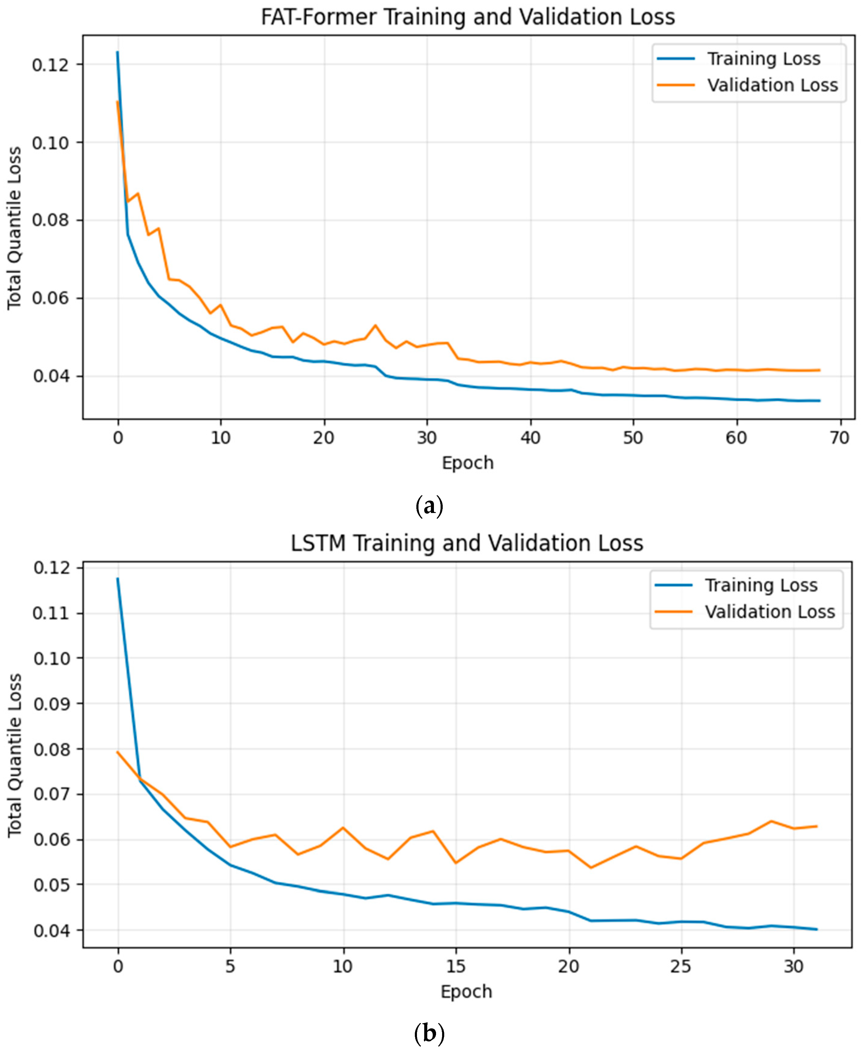
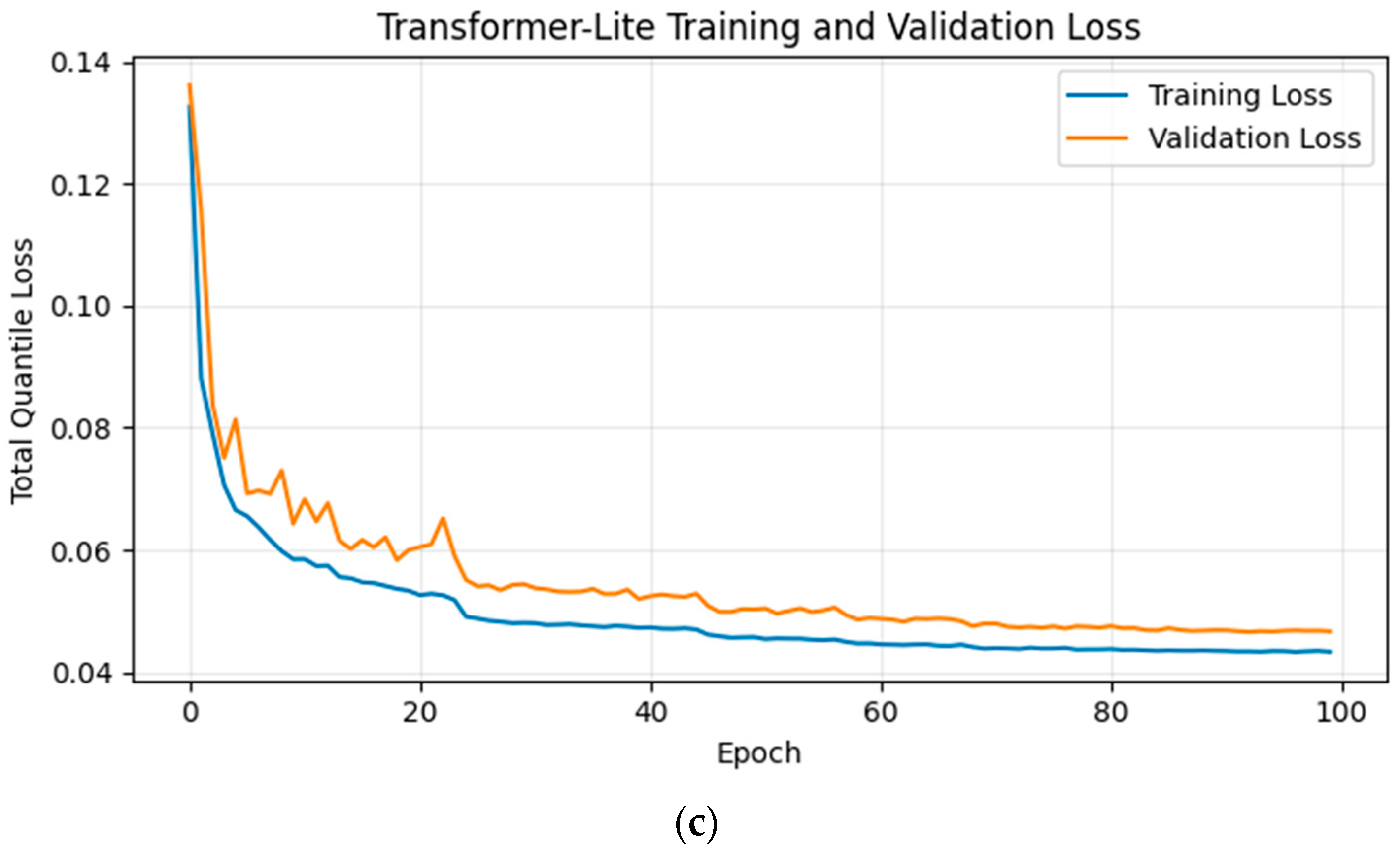
Figure 1 displays the training and validation quantile-loss behavior of FAT-Former, LSTM, and Transformer-Lite. All three models exhibited rapid loss reduction during the initial training stages, indicating successful learning of the dominant temporal structure in the input sequences. The study employed validation-based early stopping and restored the parameters corresponding to the lowest validation loss. FAT-Former reached its best validation epoch at epoch 15, compared with epoch 25 for LSTM and epoch 87 for Transformer-Lite.

Figure 1a shows the training and validation total quantile loss of the FAT-Former model. Both losses decreased rapidly during the early epochs, demonstrating effective initial learning, followed by a more gradual decline as the model approached convergence. The training loss decreased from approximately 0.123 to 0.034, while the validation loss declined from approximately 0.110 and stabilized at around 0.041. Minor fluctuations in the validation loss were observed during the intermediate epochs; however, no sustained increase occurred. The small and relatively stable separation between the training and validation curves suggests that the model generalized well to unseen validation data, with no indication of severe overfitting. The stabilization of the validation loss after approximately 35–40 epochs further indicates that the FAT-Former had largely converged, with only marginal gains obtained from subsequent training epochs.

Figure 1b illustrates the training and validation total quantile loss of the LSTM model. Both losses decreased rapidly during the initial epochs, indicating effective early learning. The training loss continuously declined from approximately 0.118 to 0.040 throughout the training process. In contrast, the validation loss initially decreased but subsequently fluctuated between approximately 0.054 and 0.064. The minimum validation loss was observed at approximately epoch 21, after which it gradually increased while the training loss continued to decline. The growing separation between the training and validation curves indicates that the LSTM began to overfit the training data during the later stages of training. These results suggest that early stopping at or near the minimum validation loss may provide better generalization performance and prevent unnecessary fitting of training-specific patterns.

Figure 1c reveals the training and validation total quantile loss of the Transformer-Lite model. Both losses decreased sharply during the initial training epochs, indicating rapid learning of the underlying temporal patterns. The training loss decreased from approximately 0.133 to 0.043, while the validation loss declined from approximately 0.136 and stabilized at approximately 0.046–0.047 toward the end of training. Although minor fluctuations were observed in the validation loss during the early and intermediate epochs, these were temporary and were followed by a continued downward trend. The relatively small and stable gap between the training and validation curves suggests that the Transformer-Lite achieved good generalization with minimal evidence of overfitting. Furthermore, the stabilization of both curves during the later epochs indicates that the model successfully converged.

Independent-Test Point Forecasting Performance

Table 1. Independent-Test Point Forecast Performance.

Model	RMSE (Wh/m2)	MAE (Wh/m2)	R2	WAPE (%)	nRMSE (%)
Persistence	98.7986	62.0447	0.8778	30.3142	9.8042
LSTM	32.6458	15.6367	0.9867	7.6399	3.2396
Transformer-Lite	31.5617	14.6898	0.9875	7.1773	3.1320
FAT-Former	31.1755	13.3501	0.9878	6.5227	3.0937

exhibits the deterministic forecasting performance evaluated on the same independent test timestamps for all models.

FAT-Former substantially improved forecasting accuracy relative to the persistence benchmark. Its RMSE decreased from 98.7986 Wh/m² to 31.1755 Wh/m², corresponding to an approximate 68.45% reduction in RMSE. Similarly, MAE decreased from 62.0447 Wh/m² to 13.3501 Wh/m², representing an approximate 78.48% reduction. The coefficient of determination increased from R² = 0.8778 for persistence to R² = 0.9878 for FAT-Former.

These improvements indicate that the multivariate 24 h input sequence captures temporal and atmospheric information that cannot be represented adequately by persistence alone. This distinction is particularly important for irradiance forecasting under rapidly changing local atmospheric conditions. Persistence inherently assumes that irradiance conditions remain relatively unchanged between consecutive forecasting intervals. Such an assumption becomes restrictive when cloud development, precipitation, humidity variation, and other localized atmospheric processes produce abrupt changes in solar irradiance. By incorporating the temporal behavior of multiple predictors over the preceding 24 h, the learned models are better able to represent these evolving conditions and anticipate short-term irradiance transitions.

Among the learned models, FAT-Former achieved the lowest aggregate prediction error. It obtained an RMSE of 31.1755 Wh/m², MAE of 13.3501 Wh/m², WAPE of 6.5227%, and nRMSE of 3.0937%, together with the highest $R^2$ of 0.9878. Relative to the LSTM, FAT-Former reduced RMSE by approximately 4.50% and MAE by 14.62%. Compared with Transformer-Lite, the improvements were smaller but still consistent, with reductions of approximately 1.22% in RMSE and 9.12% in MAE. FAT-Former also marginally improved $R^2$ from 0.9875 for Transformer-Lite to 0.9878.

The consistently superior performance of FAT-Former across all evaluation metrics provides empirical support for the proposed architecture. Although Transformer-Lite also achieved competitive results, FAT-Former obtained the lowest RMSE, MAE, WAPE, and nRMSE, together with the highest $R^2$, demonstrating that the additional modeling capacity incorporated in the FAT-Former architecture contributes to more accurate one-hour-ahead solar irradiance forecasting. In particular, the improvement in MAE indicates that FAT-Former produces smaller absolute prediction errors. At the same time, the lower WAPE and nRMSE demonstrate improved accuracy relative to the magnitude and variability of the observed irradiance values. These consistent gains over both LSTM and Transformer-Lite establish FAT-Former as the best-performing learned model evaluated in this study.

Importantly, the findings support the suitability of FAT-Former for extracting predictive information from the preceding 24 h multivariate sequence. Its architecture enables the model to capture temporal dependencies and interactions among meteorological and irradiance-related variables that influence short-term solar irradiance behavior. While the performance difference between FAT-Former and Transformer-Lite is relatively small for RMSE and $R^2$, FAT-Former maintains a consistent advantage across all reported metrics, particularly in MAE and WAPE. Taken collectively, these results provide quantitative evidence supporting FAT-Former as the proposed model for one-hour-ahead solar irradiance forecasting under the conditions investigated in this study.

4.2. Daylight-Only Performance

Because solar irradiance approaches zero during the nighttime, full-period error measures may benefit from many comparatively easy zero or near-zero predictions. Daylight-only evaluation presented in

Table 2. Daylight-only point forecast performance.

Model	RMSE (Wh/m2)	MAE (Wh/m2)	(R2)	WAPE (%)	nRMSE (%)
Persistence	137.4766	118.6945	0.7587	29.7757	13.6484
LSTM	45.5569	30.1693	0.9735	7.5683	4.5228
Transformer-Lite	44.0227	27.4851	0.9753	6.8949	4.3705
FAT-Former	43.5076	25.8411	0.9758	6.4825	4.3194

therefore provides a more demanding assessment of forecasting performance during periods in which solar irradiance is operationally significant.

The results also show that the current FAT-Former configuration achieved the lowest overall prediction error among the evaluated learned models. FAT-Former obtained the lowest RMSE (43.508 Wh/m²), MAE (25.841 Wh/m²), WAPE (6.483%), and nRMSE (4.319%), while also achieving the highest $R^2$ value of 0.9758. Relative to the LSTM, FAT-Former reduced RMSE by approximately 4.50% and MAE by 14.35%. Compared with the Transformer-Lite model, the improvements were smaller, with reductions of approximately 1.17% in RMSE and 5.98% in MAE, together with a marginal increase in $R^2$ R-squared from 0.9753 to 0.9758. These results indicate that FAT-Former provides the best predictive accuracy among the evaluated models, although Transformer-Lite achieves closely comparable performance with a more compact architecture.

This finding is particularly meaningful given the relatively short 24 h input sequence employed for one-hour-ahead forecasting. The strong performance of Transformer-Lite indicates that a compact Transformer architecture can effectively represent a substantial proportion of the predictive information embedded within this temporal window. Nevertheless, the increased representational capacity of FAT-Former produces further reductions in prediction error, particularly in MAE and WAPE, demonstrating that the additional architectural complexity contributes measurable predictive gains. These results highlight a practical trade-off between model complexity and incremental forecasting improvement. Although the additional encoder capacity of FAT-Former yields relatively modest gains over Transformer-Lite, these improvements should be interpreted alongside computational cost, parameter count, training efficiency, and deployment requirements when determining the most appropriate architecture for operational solar irradiance forecasting.

4.3. Performance Under Precipitation and Non-Precipitation Conditions

To examine sensitivity to changing atmospheric conditions, the study stratified the independent test observations according to the presence or absence of precipitation as shown in

Table 3. Forecast performance under precipitation and non-precipitation conditions.

Condition	Model	n	RMSE (Wh/m2)	MAE (Wh/m2)	(R2)	WAPE (%)	nRMSE (%)
No precipitation	Persistence	422	131.772	95.485	0.87191	26.6658	13.1171
No precipitation	LSTM	422	26.2659	15.6971	0.99491	4.3837	2.61462
No precipitation	Transformer-Lite	422	18.7136	10.3829	0.99742	2.89959	1.86283
No precipitation	FAT-Former	422	16.4603	8.57489	0.998	2.39469	1.63853
Precipitation	Persistence	11,408	97.3649	60.8076	0.8768	30.5571	9.6619
Precipitation	LSTM	11,408	32.858	15.6344	0.98597	7.85662	3.26063
Precipitation	Transformer-Lite	11,408	31.938	14.8492	0.98674	7.46199	3.16933
Precipitation	FAT-Former	11,408	31.5887	13.5267	0.98703	6.79744	3.13467

.

Under non-precipitating conditions, FAT-Former achieved an RMSE of 16.4603 Wh/m² and MAE of 8.5748 Wh/m². Notably, its MAE and RMSE were lower than those of all other baseline models.

Under precipitation conditions, FAT-Former error increased to an RMSE of 31.5887 Wh/m² and MAE of 13.5267 Wh/m². The reduction in performance relative to the other neural models suggests that rapidly changing atmospheric states remain a significant challenge for the current FAT-Former configuration.

For the intended application in coastal and microclimate-sensitive areas, this result is especially relevant. It suggests that architectural depth alone may not sufficiently represent abrupt atmospheric transitions. Future development should therefore prioritize the explicit integration of meteorological variables associated with localized variability—where available—including precipitation, relative humidity, cloud-related variables, wind behavior, pressure, and solar geometry.

The result also provides a more meaningful direction for improving FAT-Former than simply increasing the number of Transformer layers. A microclimate-aware FAT-Former should exploit richer environmental information to condition the attention mechanism on the atmospheric processes responsible for irradiance variability.

4.4. Probabilistic Forecasting and Prediction-Interval Performance

A central feature of FAT-Former is its ability to provide probabilistic forecasts through continuous conditional quantile estimates. The model produces $q_{0.10}$, $q_{0.50}$, and $q_{0.90}$, where the median $q_{0.50}$, serves as the point forecast and the lower and upper quantiles define a nominal 80% prediction interval (

Table 4. Raw nominal 80% prediction-interval performance.

Model	PICP (%)	MPIW (Wh/m2)	nMPIW (%)	Interval Score
LSTM	66.846999	43.416741	4.308413	76.844015
Transformer-Lite	78.148774	46.028319	4.567570	71.223801
FAT-Former	87.979713	36.431199	3.615210	63.919233

). The same quantile-output formulation was also applied to LSTM and Transformer-Lite, enabling a fair uncertainty comparison.

FAT-Former achieved a Prediction Interval Coverage Probability (PICP) of 87.9797%. This was higher than those of LSTM and Transformer-Lite at 66.8469% and 78.1487%, thus FAT-Former provides the best empirical coverage of the nominal interval.

FAT-Former produced the narrowest prediction intervals, with an MPIW of 36.43 Wh/m² and an nMPIW of 3.62%, whereas Transformer-Lite and LSTM obtained MPIW values of 46.03 Wh/m² and 43.42 Wh/m², respectively. FAT-Former also achieved the lowest interval score of 63.92, compared with 71.22 for Transformer-Lite and 76.84 for LSTM. Taken together, these results indicate that FAT-Former provides a more favorable balance between prediction-interval coverage and interval sharpness, producing narrower uncertainty bounds while capturing a greater proportion of the observed irradiance values.

For microclimate-sensitive solar irradiance forecasting, this capability is particularly important because a single deterministic prediction cannot represent the uncertainty associated with rapidly changing atmospheric conditions. Variations in cloud cover, humidity, precipitation, and other localized meteorological processes can produce abrupt changes in irradiance that are difficult to characterize using point estimates alone. By generating prediction intervals directly through its probabilistic forecasting framework, FAT-Former provides information not only on the expected irradiance level but also on the plausible range within which future observations may occur.

The superior PICP, narrower MPIW and nMPIW, and lower interval score collectively provide additional evidence supporting the proposed FAT-Former architecture. Rather than obtaining improved coverage simply by widening its prediction intervals, FAT-Former achieves higher empirical coverage while maintaining narrower intervals than both LSTM and Transformer-Lite. This indicates greater sharpness and a more effective representation of predictive uncertainty. Thus, in addition to its superior deterministic forecasting performance, FAT-Former demonstrates a stronger capability for probabilistic solar irradiance forecasting, supporting its suitability for applications in which both forecast accuracy and uncertainty characterization are important.

Table 5. Conformally calibrated nominal 80% prediction intervals.

Model	(Wh/m2)	PICP (%)	MPIW (Wh/m2)	nMPIW (%)	Interval Score
LSTM	0.451172	81.622992	44.319085	4.397956	76.661276
Transformer-Lite	0.000000	78.148774	46.028319	4.567570	71.223801
FAT-Former	0.000000	87.979713	36.431199	3.615210	63.919233

shows the conformal calibration produced model-dependent effects on prediction-interval coverage. For the LSTM, the conformal correction increased PICP from 66.85% to 81.62%, bringing the empirical coverage close to the nominal 80% target. In contrast, Transformer-Lite and FAT-Former received zero conformal correction under the adopted calibration procedure; consequently, their test-set coverage remained unchanged at 78.15% and 87.98%, respectively. Transformer-Lite therefore remained slightly below the nominal coverage level, whereas FAT-Former continued to exhibit conservative coverage above the 80% target.

These results indicate that a fixed conformal calibration derived from the validation period does not affect all forecasting architectures uniformly. In a microclimate-sensitive environment, this behavior is relevant because the statistical characteristics of irradiance and associated atmospheric variables may change over time. Temporal variations in cloud cover, humidity, precipitation, and other localized meteorological conditions can alter both forecast errors and uncertainty distributions between the calibration and independent test periods. Consequently, adaptive, rolling, seasonal, or weather-conditioned conformal calibration may provide a more responsive mechanism for maintaining prediction-interval coverage under changing atmospheric regimes.

Nevertheless, FAT-Former retained the strongest overall probabilistic performance after conformal calibration. Despite its coverage exceeding the nominal 80% level, it produced the narrowest prediction intervals and the lowest interval score among the evaluated models. This indicates that its comparatively high coverage was not achieved simply by generating excessively wide intervals, but rather through a more favorable balance between coverage and interval sharpness.

4.5. Independent-Test Forecast Behavior

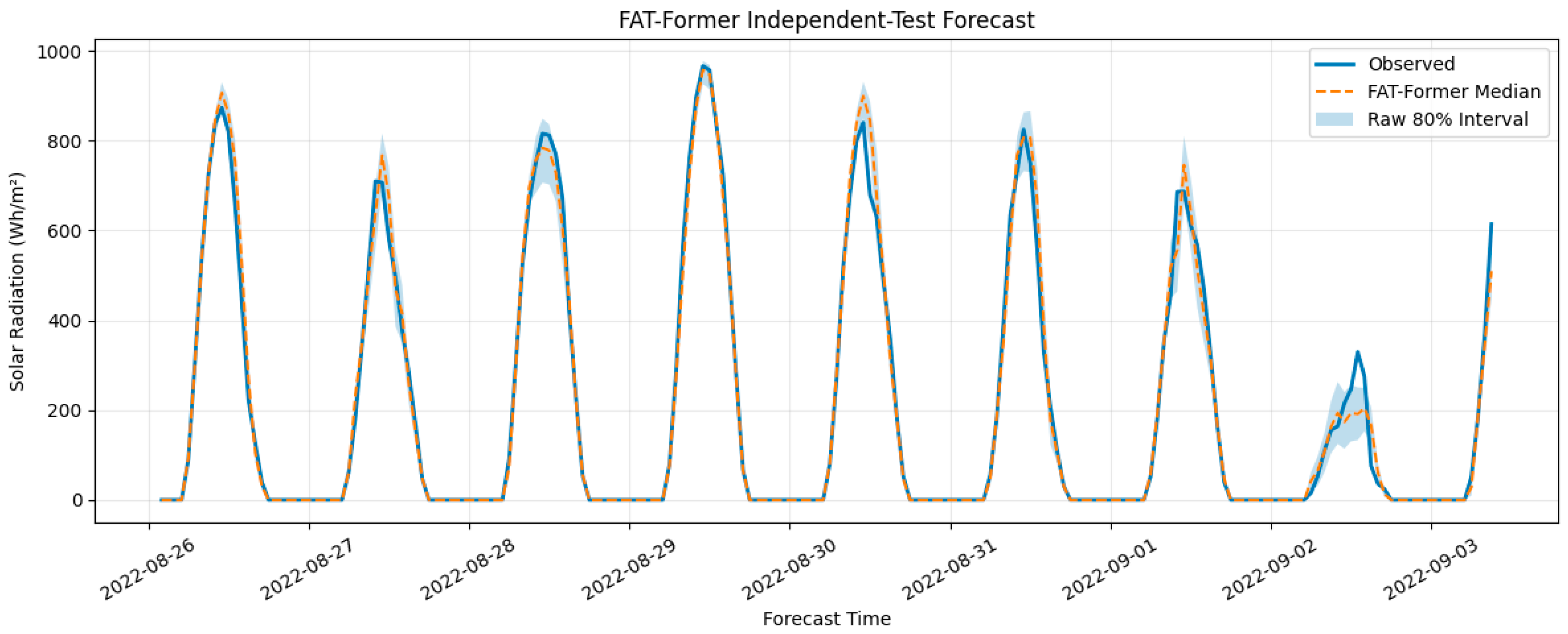
Figure 2 presents a representative section of the independent test period showing the observed irradiance, FAT-Former median prediction, and nominal 80% prediction interval.

The plotted results show that FAT-Former successfully reproduces the fundamental diurnal irradiance pattern. The median forecast follows the transition from nighttime zero irradiance to daytime irradiance and reproduces the approximate timing of daily maxima. The prediction interval expands substantially during daylight hours and contracts near nighttime zero values, which is consistent with the greater forecasting uncertainty associated with daytime atmospheric variability.

Figure 2 above also reveals important limitations. On relatively smooth days, the predicted daily profile follows the observations closely. In contrast, sudden intraday decreases in measured irradiance are not always reproduced with equivalent magnitude. The model tends to produce smoother irradiance trajectories during these transitions. This visual behavior is consistent with the precipitation-stratified results and indicates that abrupt microclimatic changes represent a major source of forecast error.

This finding reinforces the relevance of FAT-Former to the intended research problem. The architecture captures the broad temporal structure successfully; however, improving responsiveness to localized atmospheric disturbances is necessary before claiming robust forecasting performance across highly variable coastal microclimates.

4.6. Statistical Significance of Model Differences

Diebold–Mariano testing was performed using errors computed over identical independent-test timestamps. The result was illustrated in

Table 6. Diebold–Mariano tests.

Comparison	DM Statistic	p-Value	Significant at 0.05
FAT-Former vs. Persistence	−62.401	0	TRUE
FAT-Former vs. LSTM	−4.0383	5.4 × 10−5	TRUE
FAT-Former vs. Transformer-Lite	−1.1539	0.24853	FALSE

. A negative DM statistic for FAT-Former relative to another model indicates lower mean squared forecast loss for FAT-Former, whereas a positive statistic indicates greater loss.

The strongly negative DM statistic of −62.401 against persistence confirms that FAT-Former provides a statistically significant improvement over the naïve persistence approach.

The Diebold–Mariano comparison between FAT-Former and Transformer-Lite produced a DM statistic of −1.1539 with a p-value of 0.2485. Since the p-value exceeds the 0.05 significance level, the null hypothesis of equal predictive accuracy cannot be rejected. Under the adopted loss-differential convention, the negative DM statistic indicates that FAT-Former exhibited a lower average squared forecast loss than Transformer-Lite; however, this difference was not statistically significant. Thus, although FAT-Former achieved a slightly lower RMSE than Transformer-Lite, the observed improvement cannot be considered statistically distinguishable from random variation in the independent test sample. The result therefore suggests that FAT-Former and Transformer-Lite have statistically comparable predictive accuracy, with FAT-Former retaining a modest numerical advantage in the reported error metrics.

The paired error analysis produced the same overall interpretation as shown in

Table 7. Paired t-test results.

Comparison	t-Statistic	p-Value	Significant at 0.05
FAT-Former vs. Persistence	−73.954	0	TRUE
FAT-Former vs. LSTM	−14.691	1.95 × 10−48	TRUE
FAT-Former vs. Transformer-Lite	−11.442	3.71 × 10−30	TRUE

.

The statistical analyses provide strong evidence that FAT-Former substantially outperforms Persistence and LSTM. For Transformer-Lite, however, the results are more nuanced: the paired t-test indicates a statistically significant difference, whereas the Diebold–Mariano test does not reject equal predictive accuracy. This difference may arise because the two tests assess forecast errors under different statistical assumptions, particularly with respect to the temporal dependence of forecast-loss differentials. Accordingly, the superiority of FAT-Former over Transformer-Lite is supported numerically by the lower RMSE and MAE and by the paired t-test but should be interpreted more cautiously considering the non-significant Diebold–Mariano result.

4.7. Peak Irradiance Tracking

Accurate prediction of the time and magnitude of daily irradiance peaks is important for solar resource management and short-term energy planning.

Table 8. Daily peak-tracking performance.

Model	Mean Peak-Time Error (h)	Mean Peak-Magnitude Error (Wh/m2)
Persistence	1	0.00002
LSTM	0.54361	38.6347
Transformer-Lite	0.60852	28.5271
FAT-Former	0.5639	31.1157

summarizes the peak-tracking results.

FAT-Former achieved the lowest mean peak-time error at 0.5639 h, outperforming LSTM at 0.5436 h and Transformer-Lite at 1.0000 h. This result suggests that the stacked self-attention mechanism can represent temporal positioning within the daily irradiance profile effectively.

In highly dynamic coastal environments, localized atmospheric variability can substantially alter the timing of maximum available irradiance. Consequently, a forecasting system that accurately identifies the daily irradiance peak may provide operationally meaningful information that RMSE or MAE does not fully reflect.

FAT-Former, however, produced a mid-peak-magnitude error among the learned models at 31.1157 Wh/m². The model therefore appears more successful at identifying when a peak occurs than at estimating how large that peak will be.

The near-zero persistence peak-magnitude error requires cautious interpretation because the persistence baseline introduces a one-hour temporal shift that can preserve the daily maximum magnitude despite misalignment in peak timing.

4.8. Representation of Temporal Variability

To examine whether the models excessively smooth the irradiance series,

Table 9. Variability and temporal-dynamics diagnostics.

Model	Variance Ratio (Predicted/Observed)	First-Difference Energy
Persistence	1.000000	62.049906
LSTM	0.927311	59.751835
Transformer-Lite	1.019656	63.121216
FAT-Former	1.013047	62.745361

Observed first-difference energy: 62.0499.

compared predicted variance with observed variance and calculated first-difference energy.

FAT-Former preserved approximately 101.30% of the variance of the observed irradiance series, corresponding to a variance ratio of 1.0130. This value is closer to the ideal ratio of 1.0 than those obtained by LSTM (0.9273) and Transformer-Lite (1.0197). LSTM underestimated the observed variance by approximately 7.27%, indicating some attenuation of irradiance amplitude variability, whereas Transformer-Lite slightly overestimated it by approximately 1.97%. FAT-Former exhibited only a 1.30% overestimation, indicating that it reproduced the overall amplitude variability of the observed irradiance series with high fidelity.

A similar pattern was observed in the first-difference energy, which characterizes short-term temporal variability between consecutive observations. The observed series had a first-difference energy of 62.0499, while FAT-Former obtained 62.7454, only approximately 1.12% higher than the observed value. Transformer-Lite produced a slightly higher value of 63.1212, whereas LSTM yielded a lower value of 59.7518. These results indicate that FAT-Former closely preserved the magnitude of short-term irradiance fluctuations rather than excessively smoothing abrupt temporal changes. Its slight overestimation suggests marginally greater short-term variability than observed, but the difference remains small.

For microclimate-sensitive forecasting, this finding is particularly significant because rapid irradiance fluctuations can reflect localized atmospheric processes, including transient cloud movement and short-duration weather variability. FAT-Former’s ability to reproduce both the overall variance and short-term temporal variability of the observed series indicates that the model preserves key irradiance dynamics while maintaining accurate point predictions. Combined with its strong deterministic and probabilistic performance, these diagnostic results provide further evidence that FAT-Former can effectively represent both broad temporal structures and rapid irradiance fluctuations in one-hour-ahead forecasting.

4.9. Computational Requirements

Table 10. Computational cost.

Model	Trainable Parameters	Training Time (s)	Best Validation Epoch	Mean Test Inference Time (s)	Inference-Time SD (s)
LSTM	19,395	931.676	22	2.40369	0.64486
Transformer-Lite	17,667	3217.15	93	2.34024	0.53847
FAT-Former	101,315	8229.86	59	6.57111	0.85098

presents the computational characteristics of the three neural models.

FAT-Former contained 101,315 trainable parameters, approximately 5.22 times the number in LSTM and 5.73 times that in Transformer-Lite. Its inference time was also substantially higher.

Despite this computational complexity, FAT-Former achieved its optimal validation state at 59 epochs. This indicates good convergence in terms of epoch count, but each epoch is more computationally expensive because of the three stacked multi-head attention and feedforward blocks.

The current accuracy–complexity relationship therefore suggests that FAT-Former may benefit from architectural optimization. Reducing dmodel, feedforward dimensionality, the number of attention heads, or the number of stacked encoder blocks should be investigated through ablation studies. A reduced configuration may retain the favorable temporal representation and probabilistic capability of FAT-Former while approaching or surpassing Transformer-Lite in computational efficiency and point accuracy.

4.10. Implications for Coastal and Microclimate-Sensitive Areas

Taken together, the findings demonstrate that FAT-Former offers a technically viable framework for solar irradiance forecasting in coastal and microclimate-sensitive environments, while also revealing specific conditions that warrant further model refinement.

Three findings are particularly relevant.

First, FAT-Former substantially outperformed persistence, LSTM and Transformer Lite. This confirms that explicit modeling of the preceding multivariate temporal sequence is advantageous when irradiance conditions are not temporally stationary.

Second, FAT-Former demonstrated the lowest mean peak-time error and retained 101.30% of the observed variance. These findings suggest that its deeper attention mechanism contains useful temporal information that conventional aggregate error metrics alone do not completely characterize.

Third, the results indicate that FAT-Former does not excessively smooth the irradiance signal and can retain rapid temporal variations that may reflect localized atmospheric changes. Accordingly, the primary challenge for further application in microclimate-sensitive environments is not simply to increase model capacity, but to further improve the representation of changing atmospheric regimes while preserving the strong temporal responsiveness already demonstrated by the proposed FAT-Former architecture.

Accordingly, the proposed FAT-Former should be interpreted as a feature-augmented, uncertainty-aware temporal forecasting architecture whose principal potential lies in integrating heterogeneous environmental information. In a coastal application, this architecture can be extended with site-specific atmospheric predictors so that attention weights are informed by both historical irradiance behavior and variables associated with local microclimate variability.

The strong aggregate performance of Transformer-Lite also provides an important architectural insight. For the current 24 h input and one-hour prediction horizon, a single attention layer appears sufficient to capture much of the predictable temporal structure. The deeper FAT-Former architecture may become more advantageous only when the forecasting task contains sufficient complexity, for example, richer meteorological inputs, multiple seasons, longer temporal histories, or observations from explicitly characterized coastal microclimates.

5. Conclusions

This study develops FAT-Former, a feature-augmented, encoder-only Transformer framework for one-hour-ahead solar irradiance forecasting in coastal and microclimate-sensitive environments. By integrating causal temporal and spectral features, PCA-based meteorological compression, self-attention, and quantile regression, the framework captures both deterministic irradiance dynamics and predictive uncertainty. Also, experimental results demonstrate substantial improvement over the persistence baseline, together with promising capability in temporal peak tracking and variance preservation. However, LSTM and Transformer-Lite achieve lower aggregate forecasting errors in the present experiment, indicating that further architectural refinement and the incorporation of richer microclimate-specific meteorological inputs are necessary to enhance predictive accuracy. Rather than establishing universal superiority, FAT-Former demonstrates the potential of feature-augmented Transformer architectures for localized and uncertainty-aware solar irradiance forecasting. Further validation across diverse coastal and microclimate-sensitive locations, weather regimes, and forecast horizons is warranted to assess its robustness, transferability, and broader generalizability.