Article

Small-Signal Stability Analysis Considering the Interaction Characteristics of Grid-Forming and Grid-Following Converters


1
North China Branch of State Grid Corporation of China, Beijing 100053, China
2
School of Electrical Engineering, Xi’an University of Technology, Xi’an 710054, China
*
Author to whom correspondence should be addressed.
Energies 2026, 19(18), 4447; https://doi.org/10.3390/en19184447 (registering DOI)
Submission received: 27 August 2026 / Revised: 15 September 2026 / Accepted: 16 September 2026 / Published: 20 September 2026
(This article belongs to the Section F1: Electrical Power System)

Abstract

Unlike single-converter grid-connected systems and multi-converter grid-forming (GFM) systems operating in islanded mode, grid-connected multi-converter systems comprising parallel grid-following (GFL) and GFM converters exhibit more complex internal interactions. The negative damping of GFL converters and the low-frequency inertia of GFM converters can reinforce each other, increasing the risk of wideband oscillations. Conventional impedance models do not fully account for frequency-coupling effects among converters, which can lead to impedance-model mismatch and invalidate the Nyquist criterion. Moreover, the high order of the transfer functions of multi-converter systems makes frequency sweeps difficult. Conversely, time-domain state-space models neglect the dynamics of individual control loops, resulting in inaccurate modeling and distorted parameter-sensitivity results. This paper develops a heterogeneous small-signal model that captures the full dynamics of GFM and GFL converters and uses an eigenvalue-sensitivity criterion to reveal their behavior under coupled parameters. On this basis, the effects of GFM inertia and damping on GFL variables, as well as the effect of phase-locked loop (PLL) bandwidth on the eigenvalues of the GFM system, are investigated. The proposed model and associated stability analysis provide a basis for assessing the stability of such systems and optimizing system parameters. Finally, simulations verify the conclusions.

1. Introduction

To accelerate the development of a clean, low-carbon, safe, and efficient new power system, grid-following (GFL) converters have become dominant in renewable-energy grid-integration systems because of their fast response. However, as renewable-energy penetration continues to increase, the grid gradually weakens, and system inertia and damping continuously decrease, thereby reducing the grid-support capability and system stability [1]. By emulating synchronous generators, grid-forming (GFM) converters can provide voltage support to the grid. A hybrid connection of GFM and GFL converters can combine the advantages of both [2]; therefore, hybrid GFL-GFM configurations are expected to become a trend in renewable-energy plants.
Although heterogeneous parallel converter systems provide both favorable dynamic response and voltage-support capabilities, the different control mechanisms of GFM and GFL converters create complex interactions among the converters [3,4]. Improving the stability of heterogeneous parallel converter systems therefore requires clarification of the mechanisms through which these interactions affect system operating characteristics.
A series of studies has investigated interactions in heterogeneous parallel converter systems. By establishing impedance models of heterogeneous systems, Refs. [5,6] showed that GFM converters provide positive damping, which can mitigate the negative damping of the PLL and improve the stability of heterogeneous parallel converter systems. Ref. [7] derived the mathematical mapping between the internal control of a converter and its external impedance, showing that the negative damping provided by the phase-locked loop (PLL) within its bandwidth affects the interaction between the active-power synchronization loop of the GFM converter and the grid, thereby degrading system stability in the low-frequency range. Ref. [8] reported that, when the PLL bandwidth is low, the interaction between the power-synchronization controller of the GFM converter and the PLL of the GFL converter can destabilize the system. These studies indicate that appropriate coordination between GFM and GFL converters can improve system stability, whereas inappropriate parameter settings can introduce new instability risks. Accordingly, Ref. [9] established an equivalent impedance model of a heterogeneous parallel converter system and, based on the positive net damping criterion, analyzed how converter control modes and GFM energy-storage operating modes affect the damping characteristics and stability of the system. Ref. [10] developed a sequence-impedance model through harmonic linearization and used the Nyquist stability criterion to investigate the effects of the steady-state operating point and control parameters on system stability. Ref. [11] derived the transfer-function matrices of the individual converters and then obtained the closed-loop dynamic equations of the multi-converter system, revealing, from the perspective of grid strength, how the placement of grid-connected converters can improve system stability. In addition to these impedance-model-based studies of heterogeneous parallel converter systems, Refs. [12,13] established state-space models of islanded microgrids to analyze the dynamic characteristics of converter interactions. Ref. [14] used a state-space model to analyze the effects of active- and reactive-power-loop control parameters and PLL parameters on system stability. However, most of these state-space analyses concern islanded microgrids and do not fully reveal the complexity of system interactions under grid-connected conditions, particularly with a weak grid, or their distinctive effects on stability. Furthermore, Ref. [15] established a state-space model of a converter system containing both grid-forming and grid-following controls connected to a weak grid and proposed self-influence and mutual-influence components to investigate the interaction between the GFM and GFL converters. In fact, the eigenvalue stability criterion based on a state-space model and the impedance stability criterion yield consistent stability boundaries for complex eigenvalues [16]. Regarding stability enhancement, Ref. [17] indicated that the electrical characteristic parameters, line parameters, and control parameters of converters make different contributions to system stability. Ref. [18] showed that modal decoupling and reinforcement of weak points can effectively improve damping ratios across multiple frequency bands. Refs. [19,20] used state-space models to determine parameter stability boundaries by observing the trajectories of eigenvalues as parameters varied and optimized parameters at the weak nodes with the largest participation factors. Therefore, appropriate coordination of control loops and control parameters is essential for improving stability. In addition, converter-based voltage and frequency stabilization methods have also been investigated in autonomous generation systems. Ref. [21] developed an AC/DC-converter-based stabilization control system for a self-excited induction generator and verified its voltage- and frequency-regulation performance through simulations and laboratory experiments. The results indicate that the coupling between converter control and the surrounding electrical system jointly affects voltage and frequency dynamics. In addition, Ref. [22] indicated that the appropriate coordination of control loops and control parameters is essential for improving stability.
In summary, existing studies provide useful guidance for stability modeling, assessment, and parameter optimization of heterogeneous parallel converter systems, but the following limitations remain: (1) because the controls of GFL and GFM converters in a heterogeneous parallel converter system are no longer independent, an appropriate model is required to clarify the interactive effects of their control parameters; and (2) current research on heterogeneous parallel converter systems focuses mainly on islanded operation, whereas the effects of interactions on stability differ under grid-connected and weak-grid conditions. The problem investigated in this paper can therefore be summarized as follows: determine the interaction between GFL and GFM converters in a heterogeneous grid-connected parallel converter system, establish the stability boundaries under this interaction, and thereby improve control-parameter optimization.
To address these issues, this paper first establishes a detailed state-space model of a heterogeneous GFL-GFM system suitable for grid-connected operation. The model fully accounts for the coupling among the grid impedance, main circuit, and primary control loops of the two converters, including the PLL and current loop of the GFL converter and the power-synchronization and voltage loops of the GFM converter. Based on this model, the mechanisms through which the parameters of the control loops, such as the PLL bandwidth and the inertia of the power-synchronization loop, interactively affect system stability are then analyzed in depth, and the underlying relationships are identified. Finally, system stability boundaries under the interactive effects of key parameters are mapped, providing a clear theoretical basis and design guidance for coordinated parameter optimization in heterogeneous parallel converter systems.

2. Materials and Methods

2.1. Modeling of a Heterogeneous Multi-Converter System

The structure of the heterogeneous multi-converter system is shown in Figure 1. The GFM and GFL converters are connected to the point of common coupling (PCC) through their respective lines. In addition to supplying a local load, the PCC is connected to the utility grid through a line. The system is modeled below.

2.1.1. Modeling of the GFM Converter

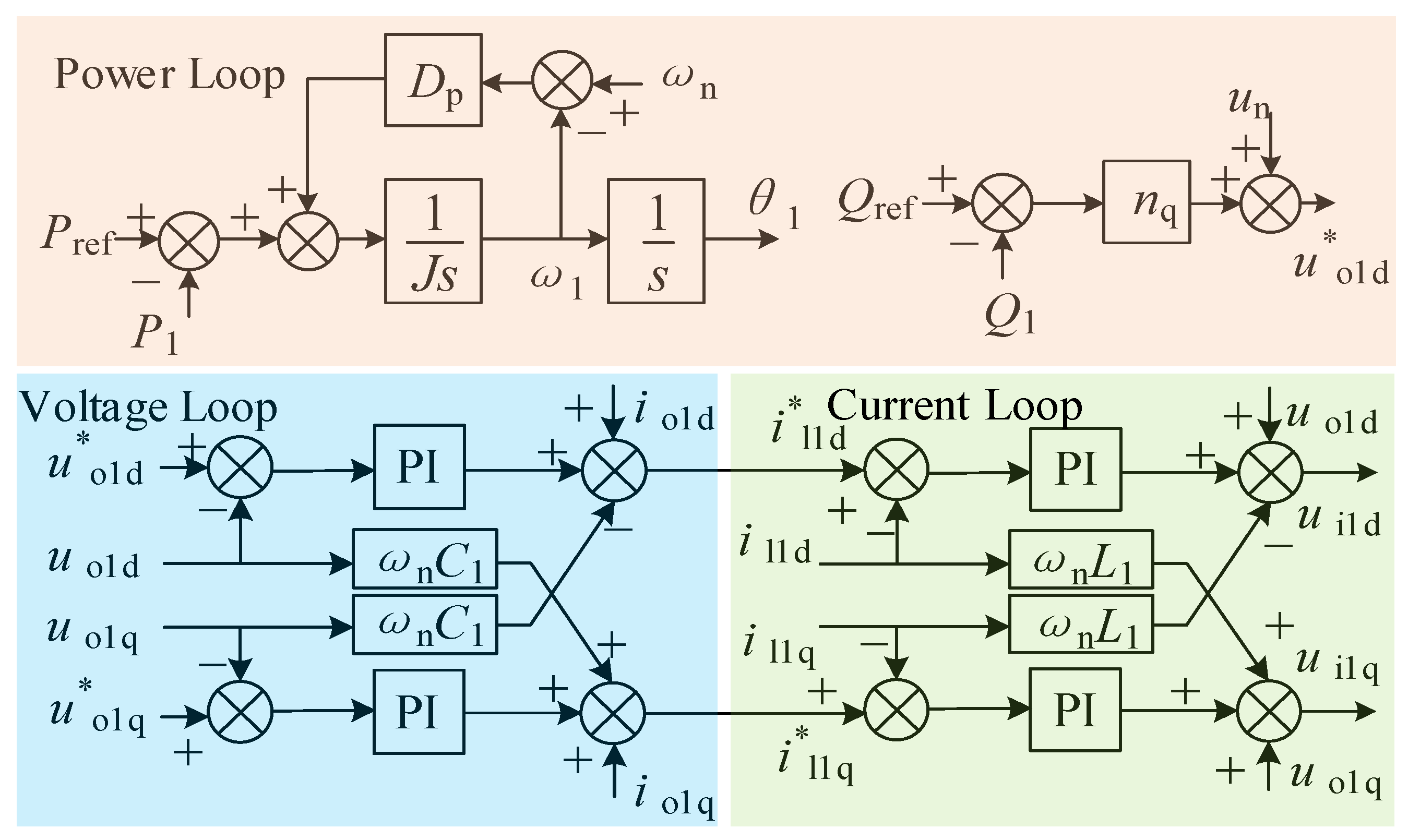
A model of the GFM converter is first established. Its control strategy, shown in Figure 2, comprises power-control, voltage-control, and current-control loops.
The power-control equations of the GFM converter are given as follows:
d ω 1 d t = 1 J ω n ( P ref P 1 ) + D p J ( ω n ω 1 ) u o 1 d * = u n + n q ( Q ref Q 1 )
where P1 and Q1 are the active- and reactive-power outputs of the GFM converter, respectively; Pref and Qref are their respective reference values; J and Dp are the virtual inertia and damping of the active-power control loop, respectively; ω1 and ωn are the actual and reference frequencies, respectively; u*o1d is the voltage output of the reactive-power loop; un is the voltage reference; and nq is the droop coefficient of the reactive-power control loop.
The output phase θ1 of the power loop is used as the phase angle of the synchronously rotating dq1 reference frame. The output voltage and current of the GFM converter are used to calculate the active and reactive powers, which are passed through low-pass filters to obtain the inputs P1 and Q1 of the power-control loop. Their expressions are as follows:
d P 1 d t = ω c P 1 + ω c ( u o 1 d i o 1 d + u o 1 q i o 1 q ) d Q 1 d t = ω c Q 1 + ω c ( u o 1 q i o 1 d u o 1 d i o 1 q )
where uo1d and uo1q and io1d and io1q are the respective components of the GFM converter output voltage and current in the dq1 reference frame, and ωc is the cutoff frequency of the low-pass filter.
d φ 1 d d t = K iv ( u o 1 d * u o 1 d ) d φ 1 q d t = K iv ( u o 1 q * u o 1 q ) i l 1 d * = i o 1 d ω n C 1 u o 1 q + K pv ( u o 1 d * u o 1 d ) + φ 1 d i l 1 q * = i o 1 q + ω n C 1 u o 1 d + K pv ( u o 1 q * u o 1 q ) + φ 1 q
The output voltage of the power loop is used as the d-axis component of the voltage reference for the voltage loop in the dq1 reference frame, whereas the q-axis component is set to zero. The voltage-control-loop equations are as follows:
Where φ1d and φ1q are the integral outputs of the proportional-integral (PI) voltage controller; Kpv and Kiv are the proportional and integral gains of the PI voltage controller, respectively; i*l1d and i*l1q are the reference currents of the current loop; and C1 is the filter capacitance.
Similarly, the current-control-loop equations are given as follows:
d γ 1 d d t = K ic 1 ( i l 1 d * i l 1 d ) d γ 1 q d t = K ic 1 ( i l 1 q * i l 1 q ) u i 1 d = u o 1 d ω n L 1 i l 1 q + K pc 1 ( i l 1 d * i l 1 d ) + γ 1 d u i 1 q = u o 1 q + ω n L 1 i l 1 d + K pc 1 ( i l 1 q * i l 1 q ) + γ 1 q
where γ1d and γ1q are the integral outputs of the PI current controller; Kpc1 and Kic1 are the proportional and integral gains of the PI current controller, respectively; ui1d and ui1q are the converter modulation voltages; and L1 is the filter inductance.
The differential equations for the variables associated with the converter-connected filter are given as follows:
d i l 1 d d t = R 1 L 1 i l 1 d + ω 1 i l 1 q + 1 L 1 u i 1 d 1 L 1 u o 1 d d i l 1 q d t = R 1 L 1 i l 1 q ω 1 i l 1 d + 1 L 1 u i 1 q 1 L 1 u o 1 q d u o 1 d d t = ω 1 u o 1 q + 1 C 1 i l 1 d 1 C 1 i o 1 d d u o 1 q d t = ω 1 u o 1 d + 1 C 1 i l 1 q 1 C 1 i o 1 q
The equations relating the output voltage and current of the GFM converter to the PCC through the line are given as follows:
d i o 1 d d t = R 3 L 3 i o 1 d + ω 1 i o 1 q + 1 L 3 u o 1 d 1 L 3 u b 1 d d i o 1 q d t = R 3 L 3 i o 1 q ω 1 i o 1 d + 1 L 3 u o 1 q 1 L 3 u b 1 q
where ub1d and ub1q are the PCC voltage components in the dq1 reference frame, and R3 and L3 are the line resistance and inductance, respectively.
The preceding equations are subjected to small-signal linearization to construct the state-space model of the GFM converter in the dq1 reference frame:
Δ x · G F M = A G F M Δ x G F M + B G F M Δ u b 1 d q
where ΔxGFM = [Δω1, ΔP1, ΔQ1, Δφ1d, Δφ1q, Δγ1d, Δγ1q, Δil1d, Δil1q, Δuo1d, Δuo1q, Δio1d, Δio1q]T is the state-variable vector of the GFM converter. The state matrix AGFM and input matrix BGFM are provided in Appendix A.

2.1.2. Modeling of the GFL Converter

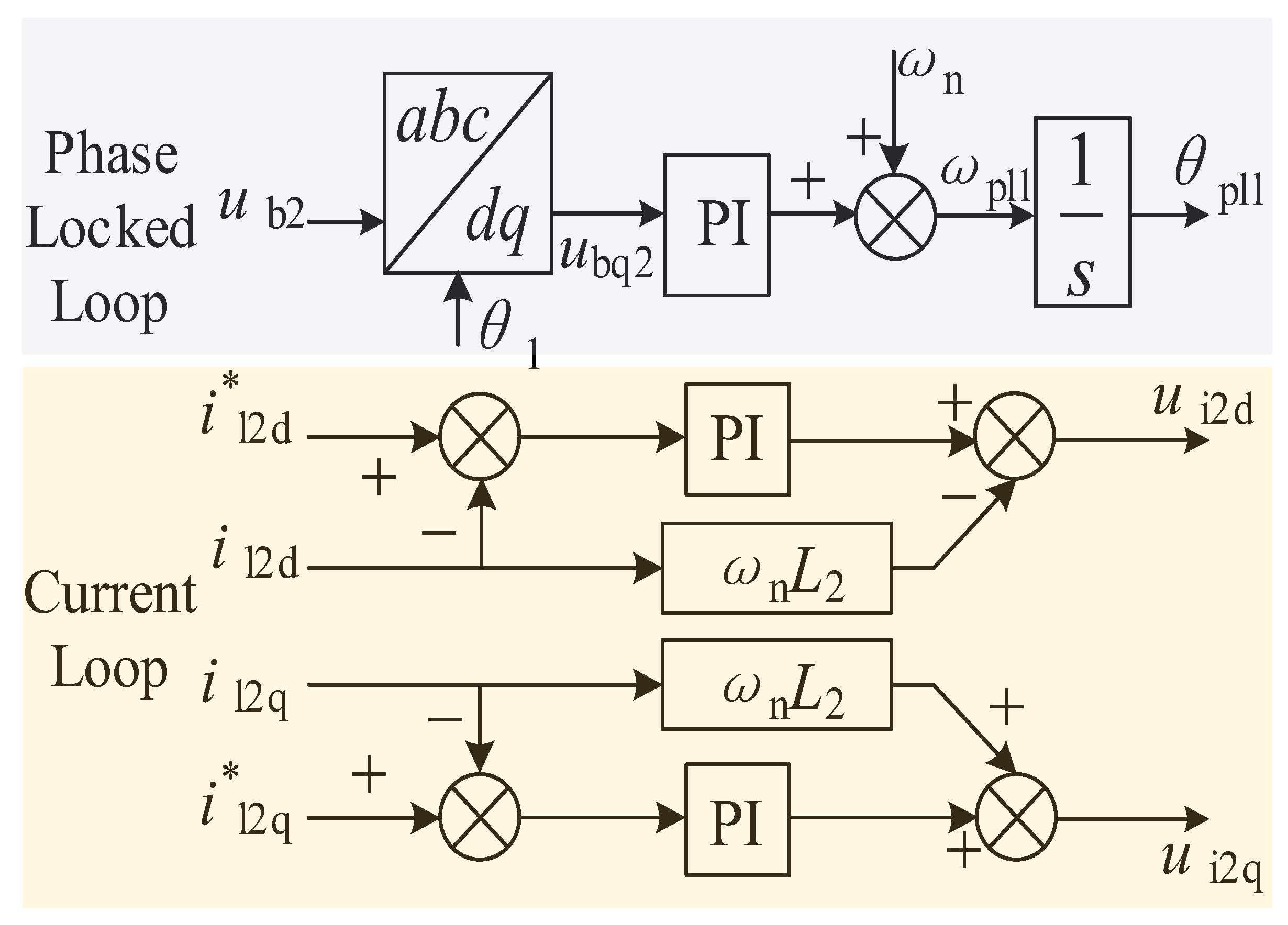
The control strategy of the GFL converter is shown in Figure 3 and comprises the PLL and current-control loops. (A dc-voltage control loop will need to be added later, although it is not used in this paper.)
The PLL synchronizes the GFL converter with the grid phase. Taking its output phase θpll as the phase angle of the synchronously rotating dq2 reference frame, the PLL control equations are written as follows:
d φ pll d t = u b 2 q d θ pll d t = ω 2 = K ppll u bq + K ipll φ pll + ω n
where ub2d and ub2q are the PCC voltage components in the dq2 reference frame; φpll is the integral output of the PI controller in the PLL; and Kppll and Kipll are the proportional and integral gains of the PI controller in the PLL, respectively.
The current-control-loop equations of the GFL converter are given as follows:
d γ 2 d d t = K ic 2 ( i l 2 d * i l 2 d ) d γ 2 q d t = K ic 2 ( i l 2 q * i l 2 q ) u i 2 d * = u o 2 d ω n L 2 i l 2 q + K pc 2 ( i l 2 d * i l 2 d ) + γ 2 d u i 2 q * = u o 2 q + ω n L 2 i l 2 d + K pc 2 ( i l 2 q * i l 2 q ) + γ 2 q
where γ2d and γ2q are the integral outputs of the PI current controller; Kpc2 and Kic2 are the proportional and integral gains of the PI current controller, respectively; u*i2d and u*i2q are the converter modulation voltages; L2 is the filter inductance; and uo2d and uo2q are the output voltages of the GFL converter.
The equations for the filter and connecting line of the GFL converter are given in Equation (11):
d i o 2 d d t = R 2 + R 4 L 2 + L 4 i o 2 d + ω 2 i o 2 q + 1 L 2 + L 4 u i 2 d 1 L 2 + L 4 u b 2 d d i o 2 q d t = R 2 + R 4 L 2 + L 4 i o 2 q ω 2 i o 2 d + 1 L 2 + L 4 u i 2 q 1 L 2 + L 4 u b 2 q
where ub2d and ub2q are the PCC voltage components in the dq2 reference frame, and R4 and L4 are the line resistance and inductance, respectively.
The small-signal linear state-space model of the GFL converter and its connecting line can likewise be derived as follows:
Δ x · G F L = A G F L Δ x G F L + B G F L Δ u b 2 d q
where ΔxGFL is the system state-variable vector of the GFL converter, ΔxGFL = [Δφpll, Δγ2d, Δγ2q, Δio2d, Δio2q]T; AGFL is the GFL system state matrix; and BGFL is the GFL system input matrix. The matrices are provided in Appendix A.

2.1.3. Modeling of the Load and Utility Grid

A resistive-inductive load is connected at the PCC. Its differential equations in the dq0 reference frame are written as Equation (14):
d i loadd d t = R load L load i loadd + ω g i loadq + 1 L load u bd d i loadq d t = R load L load i loadq ω g i loadd + 1 L load u bq
where iloadd and iloadq are the d- and q-axis current components flowing through the load, respectively; Lload and Rload are the equivalent inductance and resistance of the load, respectively; ubd and iibq are the d- and q-axis voltage components at the PCC, respectively; and ωg is the grid-voltage frequency.
The differential equations in the dq0 reference frame for the utility grid, represented by an ideal voltage source and line impedance, are given in Equation (15):
d i gd d t = R g L g i gd + ω g i gq + 1 L g u bd 1 L g u gd d i gq d t = R g L g i gq ω g i gd + 1 L g u bq 1 L g u gq
where igd and igq are the d- and q-axis current components flowing through the grid-side impedance, respectively; Lg and Rg are the equivalent inductance and resistance of the grid-side line, respectively; and ugd and ugq are the d- and q-axis voltage components at the PCC, respectively.
Small-signal linearization of the load and utility-grid models at the PCC yields the following state-space model:
Δ x · n e t = A n e t Δ x n e t + B n e t Δ u b d q 1 / L g 0 , 0 , u g d , u g q T
where Δxnet is the state-variable vector of the load and grid-side system, Δxnet = [Δiloadd, Δiloadq, Δigd, Δigq]T. Anet and Bnet are provided in Appendix A.

2.1.4. Modeling of the Heterogeneous Parallel Converter System in a Unified Reference Frame

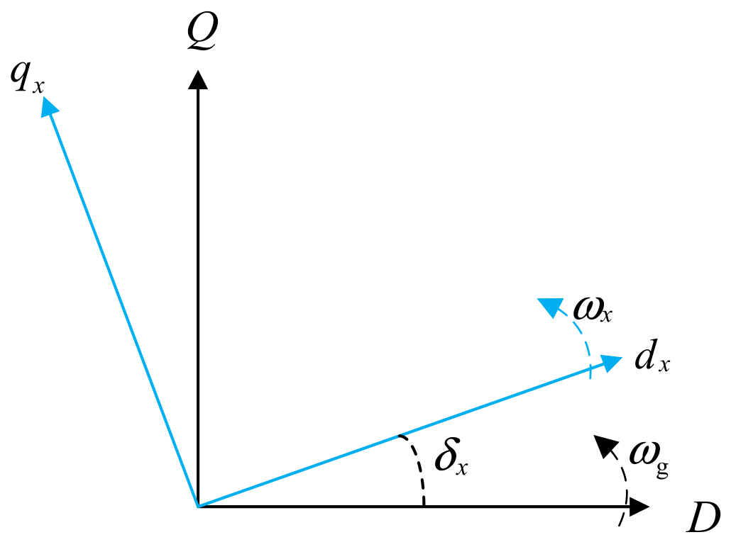
The component models developed above are formulated in different dq reference frames. The dq1 reference frame of the GFM converter uses the output phase of the power loop as its d-axis phase, whereas the GFL converter uses the PLL output as its d-axis phase. The grid line and utility-grid models use the phase of the PCC voltage vector as the d-axis reference. When the voltage is disturbed, angular differences arise among these three rotating reference frames. In this paper, a unified MG model is established in the grid-voltage-referenced rotating dq frame, which requires reference-frame transformations for both the GFM and GFL converters, as shown in Figure 4. Taking the grid-voltage dq0 reference frame as the common reference, the current io1dq injected into the PCC by the GFM converter and the current io2dq injected into the PCC by the GFL converter must be transformed into the grid-voltage reference frame, whereas the PCC voltage ubdq must be transformed into the respective rotating reference frames when modeling the GFM and GFL converters.
The angular difference δx between any individual converter and the reference frame is given by:
δ x · = ω x ω g
where ωx denotes the angular velocity of the converter’s rotating reference frame.
The current ioxdq injected into the PCC by any converter is transformed into the reference frame and denoted by ioxdq0:
i o x D i o x Q = cos δ x sin δ x sin δ x cos δ x i o x d i o x q
The PCC voltage ubdq is transformed into an arbitrary converter reference frame and denoted by ubxdq:
u b x d u b x q = cos δ x sin δ x sin δ x cos δ x u bD u bQ
From Equations (16) and (17), the small-signal state-space models for the reference-frame transformations of the output current and PCC voltage are obtained as follows:
Δ i o x D Δ i o x Q = T c 1 Δ i o x d Δ i o x q + T c 2 Δ δ x
Δ u b x d Δ u b x q = T s 1 Δ u bd Δ u bq + T s 2 Δ δ x
The coordinate-transformation matrices, including Tc1, are provided in Appendix A.
As shown by Equations (7), (11) and (14), the PCC node voltage is an input to the system. To resolve the algebraic-loop problem associated with the node-voltage equation in state-space modeling and ensure a well-conditioned numerical solution for the matrix, a virtual resistance Rn to ground is introduced. If Rn is sufficiently large, its effect on the system can be neglected, and the models of the preceding components can be unified. After introducing the virtual resistance to ground, the node equation at the PCC is given as follows:
u bd = R n i o 1 d 0 + i o 2 d 0 i loadd i gd u bq = R n i o 1 q 0 + i o 2 q 0 i loadq i gq
Combining the state-space models of the preceding components yields the following system state equation:
Δ x · s y s = A s y s Δ x s y s
where Δxsys denotes the system state-variable vector, Δxsys = [ΔxGFMT, Δδ1T, ΔxGFLT, Δδ2T, ΔxnetT], and Asys denotes the system state matrix, which is provided in Appendix A.

3. Analysis

3.1. System Stability Analysis

Based on the established state-space model of the heterogeneous MG system, the eigenvalue method is used to analyze the effects of the control parameters of the individual converters on system stability. The real part of an eigenvalue determines the decay or growth rate of the corresponding mode, whereas the imaginary part determines its oscillation frequency. The eigenvectors reflect the degree to which each system state variable participates in each mode. Each pair of complex-conjugate eigenvalues corresponds to an oscillatory mode, hereinafter referred to as a ‘mode.’ A mode characterizes the system’s intrinsic dynamic behavior in the absence of external excitation. In this study, one parameter is varied at a time, and the changes in the low-frequency eigenvalues of the state matrix are observed to identify the eigenvalues that are sensitive to that parameter. Because a parameter change may alter the steady-state operating point of the MG system, the steady-state solution of the MG system must be recalculated after each parameter change. The state matrix is then reconstructed based on the updated steady-state solution, and the eigenvalues are calculated again.
To more accurately analyze the relationship between the eigenvalues and the system state variables as the parameters vary, participation-factor analysis is introduced. For any eigenvalue λi, its right eigenvector ξi satisfies:
A ξ i = λ i ξ i ( i = 1 , 2 , , n )
where ξi = [ξ1, ξ2, …, ξi].
Similarly, the left eigenvector ψi satisfies:
Ψ i A = λ i Ψ i ( i = 1 , 2 , , n )
where ψi = [ψ1, ψ2, …, ψi].
The left and right eigenvectors associated with any eigenvalue are mutually orthogonal. The kth element of the right eigenvector ξi represents the degree of participation of the state variable xk in the ith mode, whereas the kth element of the left eigenvector represents its weight in that mode. The left and right eigenvectors obtained from the participation matrix provide a measure of the relationship between the state variables and the modes. The participation matrix can be expressed as:
P = [ P 1 , P 2 , , P n ]
where
P i = p 1 i p 2 i p m i = ξ 1 i Ψ i 1 ξ 2 i Ψ i 2 ξ m i Ψ i n
Then, it is normalized by the sum of the absolute values of all n states corresponding to the same eigenvalue:
p k i = Ψ i k · ξ k i j = 1 n Ψ i j · ξ j i
In Equation (25), pki = uki*vki is the participation factor in the participation matrix, and its magnitude represents the relative participation of the kth state variable in the ith oscillatory mode. Participation-factor analysis can be used to identify the dominant state variables associated with a given eigenvalue and thereby locate the key parameters that cause instability. This study combines eigenvalue analysis with participation-factor analysis to investigate the unstable modes induced by changes in the control parameters and their corresponding dominant state variables, thereby revealing the intrinsic mechanisms underlying the interactions within the heterogeneous parallel converter system.

3.1.1. Influence of Individual Parameters on System Stability

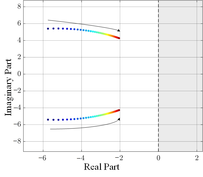
Figure 5 shows the effect of changes in the virtual inertia parameter on system stability. The analysis shows that, as J increases, the low-frequency eigenvalues move toward the right half-plane, and the decrease in the absolute values of their real parts indicates a longer dynamic response time. The continued decrease in the damping ratio not only degrades the system’s disturbance rejection capability but also increases the amplitude of post-disturbance oscillations. Excessive virtual inertia limits the GFM converter’s ability to dynamically regulate power imbalance.
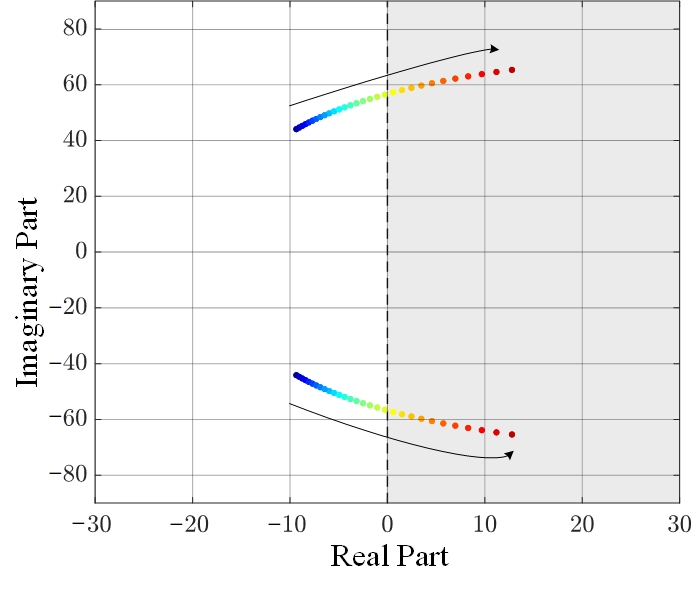
As shown in Figure 6, reducing the damping coefficient causes the low-frequency eigenvalues to gradually shift toward the imaginary axis, degrading system stability.
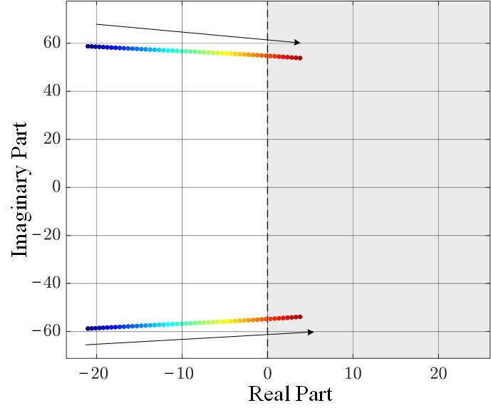
As shown in Figure 7, as the proportional gain of the GFL converter’s PLL increases from 0.8 to 5, the eigenvalues gradually cross the imaginary axis at low frequencies and enter the right half-plane, causing the system to become unstable. The high bandwidth of the PLL introduces a negative-damping effect and degrades the system’s phase margin.

3.1.2. Interaction Analysis and Coordinated Parameter Optimization

To quantitatively characterize the degree of coupling between the GFM and GFL converters in a specific oscillatory mode, this study defines a heterogeneous-system interaction factor based on the conventional participation factor:
I I i = 2   min p GFM , p GFL p GFM + p GFL
where ΣpGFM denotes the sum of the participation factors of all state variables in the GFM system for mode i; ΣpGFL is defined analogously. The index is normalized to the range [0, 1]. When IIi approaches 1, the GFM and GFL converters participate nearly equally in the oscillatory mode (strong coupling); when IIi approaches 0, the mode is dominated by one of the converters (weak coupling).
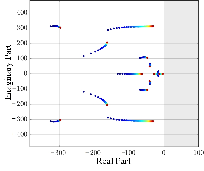
As shown in Figure 8, as the SCR decreases from 5 to 1.5, the eigenvalues of all dominant modes shift toward the right, and system stability decreases significantly. As the SCR decreases, the electrical distance between the PCC and the utility grid increases, bringing the GFM and GFL converters electrically closer and strengthening their coupling. Table 1 lists the heterogeneous-system interaction factors of the dominant modes at an SCR of 1.5. All interaction factors exceed 0.5, indicating that both the GFM and GFL converters exhibit high participation in the dominant modes.
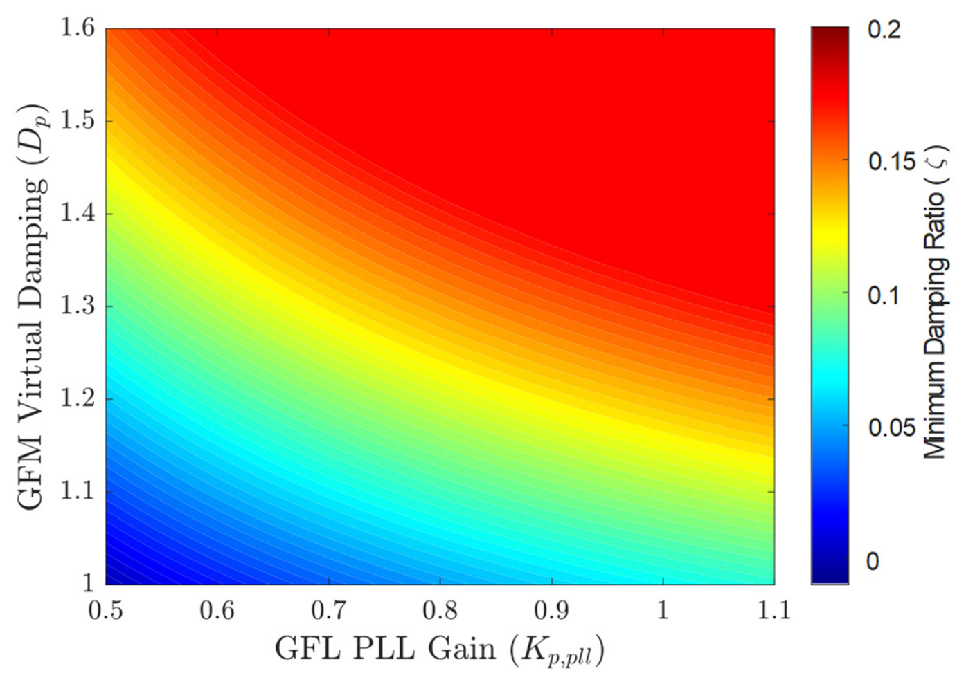
To quantify this coupling, a Dp-Kppll stability heatmap is constructed for the weak-grid condition with SCR = 2, as shown in Figure 9. The red region represents a high-damping stable region, whereas the blue region represents a low-damping unstable region. The figure shows that the GFL converter’s Kppll introduces negative damping, whereas the GFM converter’s Dp provides positive damping. To maintain the same level of system stability when increasing the tracking speed of the GFL converter, the virtual damping of the GFM converter must be increased correspondingly for compensation.
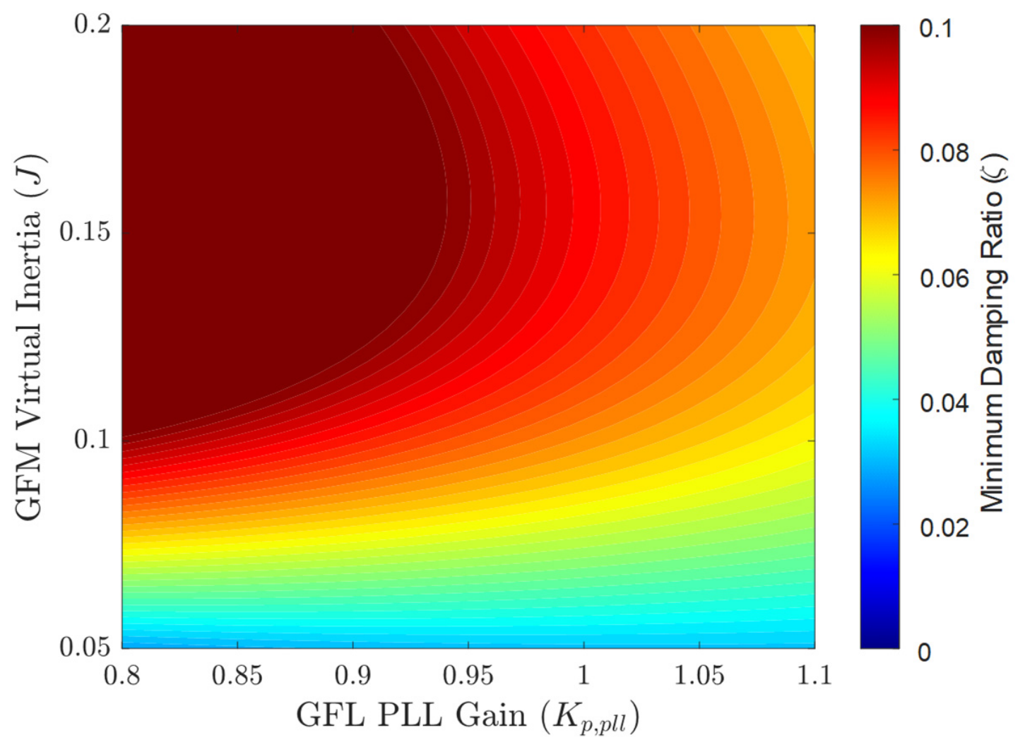
The coupling between J and Kppll is further analyzed. Figure 10 shows the J-Kppll stability heatmap. A distinct unstable region appears in the lower-right corner of Figure 10, whereas increasing J can significantly expand the stable range of Kppll. A larger J shifts the dynamic response of the GFM converter toward lower frequencies, thereby avoiding the mid-frequency bandwidth of the PLL in the frequency domain and weakening the dynamic interaction. Figure 4 and Figure 10 show that J should be neither excessively large nor excessively small. The system’s dynamic response time should be minimized while avoiding the PLL bandwidth.

4. Simulation Validation

Based on the above analysis, a simulation test system is constructed according to the system configuration shown in Table 2 to verify the validity of the stability analysis presented in this paper. Specifically, a grid-forming (GFM) converter and a grid-following (GFL) converter are connected in parallel to the PCC through transmission lines. A local RL load is also connected to the PCC, together with the main grid, which is equivalently represented by a line and an ideal voltage source.
Table 2. Circuit and control parameters of the heterogeneous parallel converter system.
CategoryParameterValue
GFM parametersPref/W8000
Qref/var6000
J0.05
Dp15
nq/V/Var0.00156
Kpv0.5
Kiv200
Kpc125
Kic21000
L1/mH2
R10.02
C1/μF50
L3/mH3
R30.1
GFL parametersPref/W9330
Qref/var0
Kppll0.8
Kipll10
Kpc20.7
Kic210
i*l2d/A20
L2/mH5
R20.05
L4/mH2
R40.06
Grid-side parametersLg/mH0.2
Rg0.5
ug/V311
Load parametersRload7.11
Lload/mH22.6
The meaning of “*” is that the value is a reference value.

Simulation Validation of the Interaction Between the GFM and GFL Converters

To validate the conclusions regarding the interaction characteristics between the GFM and GFL converters analyzed in Section 3.1, the same parameters as those used in the analysis in Section 3.1.1 are adopted, while all other parameters are held constant. The parameters are adjusted according to the variation patterns described in Section 3.1, and the corresponding output-current waveforms are observed.
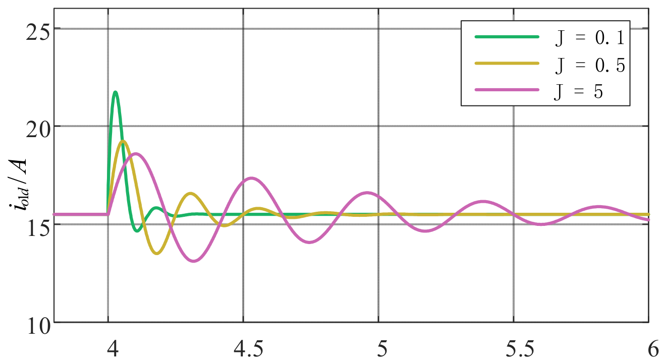
Three values of J (5, 0.5, and 0.1) are considered. A grid-side disturbance is applied at t = 4 s, and the d-axis output current of the GFM converter is shown in Figure 11. The larger the inertia, the longer the time required for the system to regain stability.
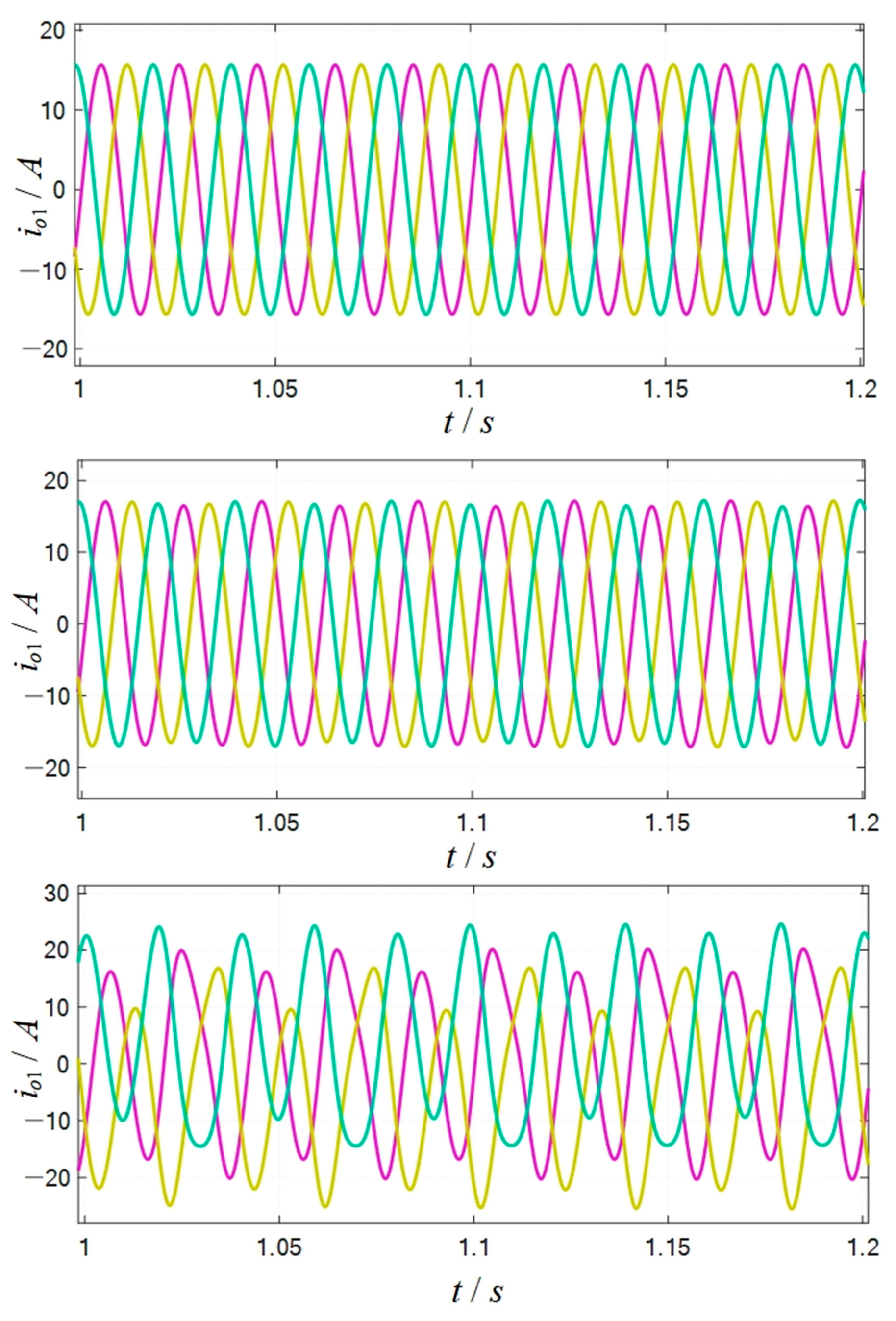
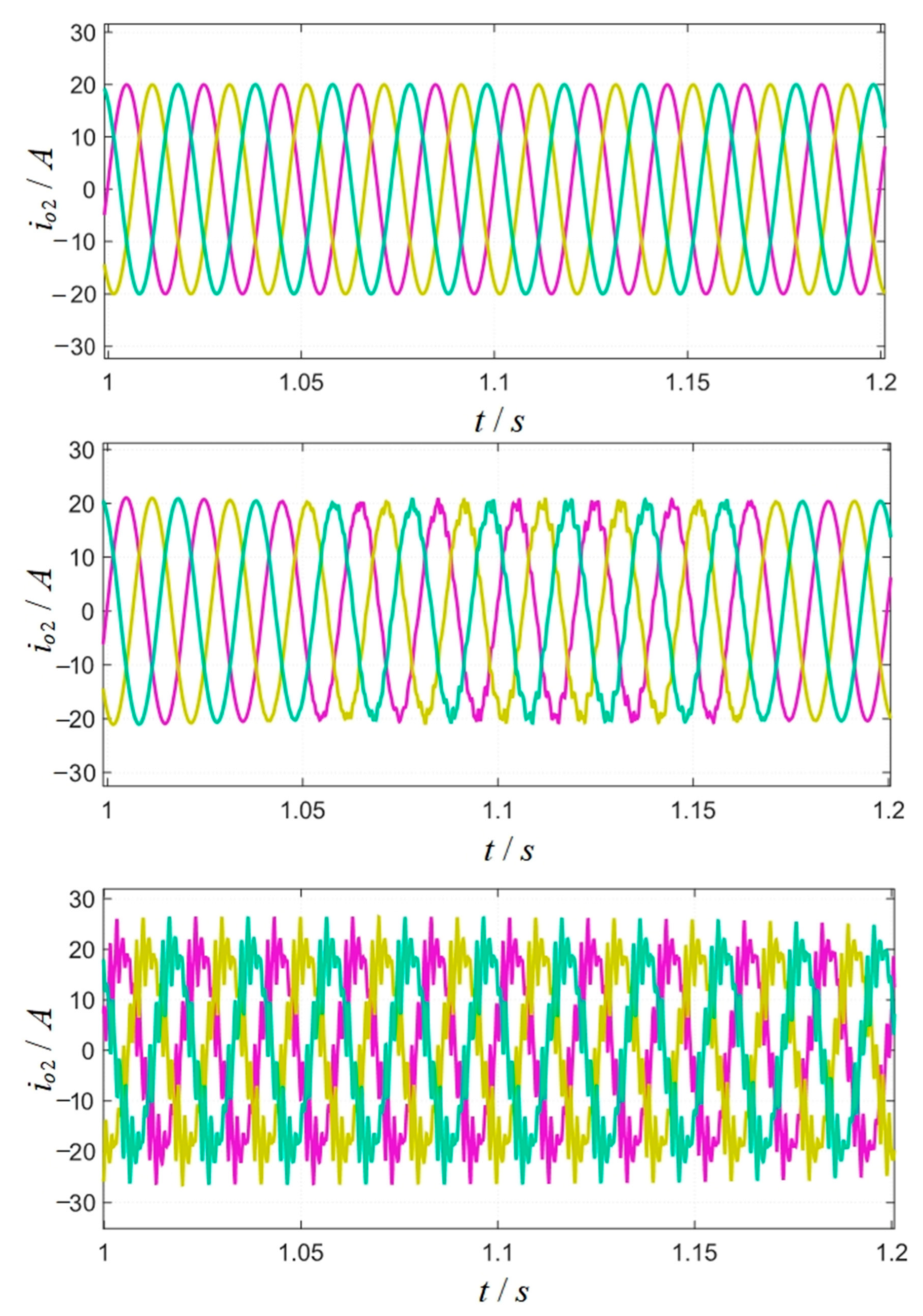
Figure 12 shows the output-current waveforms of the GFL converter for Dp = 15, Dp = 2.5, and Dp = 1. As the damping coefficient decreases, the power quality of the GFL converter’s output current progressively deteriorates, and its harmonic content gradually increases.
Figure 13 shows the output-current waveforms of the GFL converter at different PLL proportional gains. As Kppll increases, the current no longer remains a constant-amplitude sinusoidal waveform; instead, its amplitude undergoes severe periodic fluctuations.
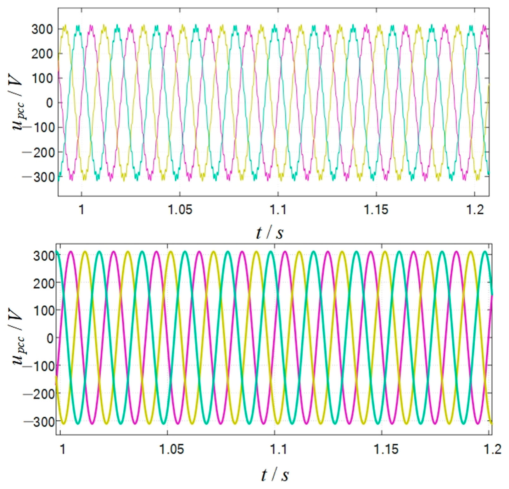
To verify the parameter-optimization pattern under weak-grid conditions analyzed in Section 3.1, this section compares the current waveforms obtained with different parameter sets under a weak-grid condition. Simulations are performed using the parameters listed in Table 3. Figure 14a shows the PCC voltage waveform at SCR = 2.2. The parameters are then optimized according to the parameter-optimization pattern presented in Section 3.1.2. Figure 14b shows the PCC voltage waveform obtained with the new parameters.

5. Conclusions

This study addresses the interaction stability of a parallel system comprising a grid-forming (GFM) converter and a grid-following (GFL) converter under weak-grid conditions and establishes a small-signal state-space model that incorporates the complete control chain. By combining eigenvalue and participation-factor analyses with a subsystem interaction factor and stability heatmaps, the dynamic coupling mechanism between the heterogeneous converters is quantified. Theoretical analysis and time-domain simulations yield the following main conclusions:
The high-bandwidth PLL of the GFL converter introduces a significant negative-damping effect, whereas the virtual damping D_p of the GFM converter provides essential positive-damping support. To accommodate a higher GFL tracking speed, D_p of the GFM converter must be increased simultaneously to offset the negative-damping effect.
A larger virtual inertia J is not necessarily more beneficial for the GFM converter. This study demonstrates that inertia does not have a monotonically beneficial effect on stability; excessive inertia slows the dynamics of the GFM converter and causes its dynamic-response frequency to fall within the unstable bandwidth range of the PLL. When designing the parameters, the system’s dynamic response time should be minimized while avoiding the PLL bandwidth.

Author Contributions

Conceptualization, C.W., X.Z. and J.L.; methodology, C.W., X.Z. and J.L.; software, C.W. and J.L.; validation, W.Z., Y.W. and X.Z.; formal analysis, C.W. and X.Z.; investigation, C.W., W.Z. and Y.W.; resources, W.Z. and Y.W.; data curation, C.W. and W.Z.; writing—original draft preparation, C.W. and J.L.; writing—review and editing, W.Z., Y.W., X.Z. and J.L.; visualization, C.W. and J.L.; supervision, X.Z.; project administration, W.Z. and Y.W.; funding acquisition, W.Z. and Y.W. All authors have read and agreed to the published version of the manuscript.

Funding

This research was funded by the Technical Research Service Project of the North China Branch of State Grid Corporation of China, “Research on the Influence Mechanism of Unit Control Parameters, and Modeling Methods and Stability Strategies for Multi-Machine Systems in Renewable Energy Stations” (Grant No. B7992326Z01D).

Data Availability Statement

The data supporting the findings of this study are included in the article. Additional model parameters, simulation files, and supporting data are available from the corresponding author upon reasonable request.

Conflicts of Interest

Authors Cong Wang, Wei Zhao and Yuzhi Wang were employed by the North China Branch of State Grid Corporation of China. The remaining authors declare that the research was conducted in the absence of any commercial or financial relationships that could be construed as potential conflicts of interest. The authors declare that this study received funding from the North China Branch of State Grid Corporation of China. The funder’s involvement was limited to the contributions of its affiliated authors, as described in the Author Contributions statement.

Appendix A

Appendix A.1. State and Input Matrices of the GFM System

A G F M = A p 0 3 × 4 A p _ f 1 A c 1 _ p 0 4 × 4 A c 1 _ f 1 A f 1 _ p A f 1 _ c 1 A f 1
A p = D p J 1 J ω n 0 0 ω c 0 0 0 ω c
A p _ f 1 = ω c 0 0 0 0 0 0 0 0 I o 1 d 0 I o 1 q 0 U o 1 d 0 U o 1 q 0 0 0 I o 1 q 0 I o 1 d 0 U o 1 q 0 U o 1 d 0
A c 1 _ p = 0 0 K i v n q 0 0 0 0 0 K i c 1 K i v n q 0 0 0
A c 1 _ f 1 = 0 0 K i v 0 0 0 0 0 0 K i v 0 0 K i c 1 0 K i c 1 K p v 0 0 0 0 K i c 1 0 K i c 1 K p v 0 0
A f 1 _ p = I l 1 q 0 0 K p c 1 K p v n q L 1 I l 1 d 0 0 0 U o 1 q 0 0 0 U o 1 d 0 0 0 I o 1 q 0 0 0 I o 1 d 0 0 0
A f 1 _ c 1 = K p c 1 L 1 0 1 L 1 0 0 K p c 1 L 1 0 1 L 1 0 0 0 0 0 0 0 0 0 0 0 0 0 0 0 0
A f 1 = R 1 + K p c 1 L 1 ω 0 K p c 1 K p v L 1 0 0 0 ω 0 R 1 + K p c 1 L 1 0 K p c 1 K p v L 1 0 0 1 C 1 0 0 ω 0 1 C 1 0 0 1 C 1 ω 0 0 0 1 C 1 0 0 1 L 3 0 R 3 L 3 ω 0 0 0 0 1 L 3 ω 0 R 3 L 3
B G F M = 0 1 × 11 , 1 L 3 , 0 ; 0 1 × 11 , 1 L 3 T

Appendix A.2. State and Input Matrices of the GFL System

A G F L = 0 0 0 0 0 0 0 0 K i c 2 0 0 0 0 0 K i c 2 I o 2 q 0 k i _ p l l 1 L 2 + L 4 0 R 2 + R 4 + K p c 2 L 2 + L 4 ω 0 L 4 L 2 + L 4 I o 2 d 0 k i _ p l l 0 1 L 2 + L 4 ω 0 L 4 L 2 + L 4 R 2 + R 4 + K p c 2 L 2 + L 4
B G F L = 0 1 0 0 0 0 0 I o 2 q 0 k p _ p l l L e q 2 0 I o 2 d 0 k p _ p l l L e q 2
u o 2 d = L 4 d i o 2 d d t + u b 2 d + R 4 i o 2 d ω 2 L 4 i o 2 q u o 2 q = L 4 d i o 2 q d t + u b 2 q + R 4 i o 2 q + ω 2 L 4 i o 2 d

Appendix A.3. State and Input Matrices of the Load and Grid

A n e t = R l o a d L l o a d ω 0 0 0 ω 0 R l o a d L l o a d 0 0 0 0 R g L g ω 0 0 0 ω 0 R g L g
B n e t = 1 L l o a d 0 0 1 L l o a d 1 L g 0 0 1 L g

Appendix A.4. Coordinate Transformation Matrices

T c 1 = cos   δ 0 x sin   δ 0 x sin   δ 0 x cos   δ 0 x T c 2 = ( sin   δ 0 x I o x d + cos   δ 0 x I o x q ) cos   δ 0 x I o x d sin   δ 0 x I o x q T s 1 = cos   δ 0 x sin   δ 0 x sin   δ 0 x cos   δ 0 x T s 2 = sin   δ 01 U b D + cos   δ 01 U b Q cos   δ 01 U b D sin   δ 01 U b Q

Appendix A.4.1. GFM

T c 11 = cos   δ 01 sin   δ 01 sin   δ 01 cos   δ 01 T c 21 = ( sin   δ 01 I o 1 d + cos   δ 01 I o 1 q ) cos   δ 01 I o 1 d sin   δ 01 I o 1 q T s 11 = cos   δ 01 sin   δ 01 sin   δ 01 cos   δ 01 T s 21 = sin   δ 01 U b D + cos   δ 01 U b Q cos   δ 01 U b D sin   δ 01 U b Q

Appendix A.4.2. GFL

T c 31 = cos   δ 02 sin   δ 02 sin   δ 02 cos   δ 02 T c 41 = ( sin   δ 02 I o 2 d + cos   δ 02 I o 2 q ) cos   δ 02 I o 2 d sin   δ 02 I o 2 q T s 31 = cos   δ 02 sin   δ 02 sin   δ 02 cos   δ 02 T s 41 = sin   δ 02 U b D + cos   δ 02 U b Q cos   δ 02 U b D sin   δ 02 U b Q

Appendix A.5. State Matrix of the Parallel System

A s y s = A 11 A 12 A 13 A 14 A 15 P ω 1 0 0 0 0 A 31 A 32 A 33 A 34 A 35 A 41 A 42 A 43 A 44 A 45 A 51 A 52 A 53 A 54 A 55
A 11 = A G F M + B G F M T s 1 R n T c 1 C i 1 A 12 = B G F M ( T s 1 R n T c 2 + T s 2 ) A 13 = B G F M T s 1 R n T c 3 C i 2 A 14 = B G F M T s 1 R n T c 4 A 15 = B G F M T s 1 R n C i n e t A 31 = B G F L T s 3 R n T c 1 C i 1 A 32 = B G F L T s 3 R n T c 2 A 33 = A G F L + B G F L T s 3 R n T c 3 C i 2 A 34 = B G F L ( T s 3 R n T c 4 + T s 4 ) A 35 = B G F L T s 3 R n C i n e t A 41 = K P T s 3 R n T c 1 C i 1 A 42 = K P T s 3 R n T c 2 A 43 = k i _ p l l P ϕ p l l + K P T s 3 R n T c 3 C i 2 A 44 = K P ( T s 3 R n T c 4 + T s 4 ) A 45 = K P T s 3 R n C i n e t A 51 = B n e t R n T c 1 C i 1 A 52 = B n e t R n T c 2 A 53 = B n e t R n T c 3 C i 2 A 54 = B n e t R n T c 4 A 55 = A n e t B n e t R n C i n e t
C i 1 = 0 0 0 0 0 0 0 0 0 0 0 1 0 0 0 0 0 0 0 0 0 0 0 0 0 1
C i 2 = 0 0 0 1 0 0 0 0 0 1
C i n e t = 1 0 1 0 0 1 0 1
P ω 1 = 1 0 0 0 0 0 0 0 0 0 0 0 0
P φ p l l = 1 0 0 0 0
K p = 0 k p p l l

References

  1. Xu, Z. Three major technical challenges facing power grids with a high proportion of nonsynchronous-machine power sources. South. Power Syst. Technol. 2020, 14, 1–9. (In Chinese) [Google Scholar] [CrossRef]
  2. Rosso, R.; EngelKen, S.; Liserre, M. Robust Stability Investigation of the Interactions Among Grid-Forming and Grid-Following Converters. IEEE J. Emerg. Sel. Top. Power Electron. 2020, 8, 991–1003. [Google Scholar] [CrossRef] [Scilit]
  3. Zhan, X.; Yuan, H.; Hu, G.; Xin, H. Low-frequency small-signal stability analysis of hybrid systems comprising grid-following and grid-forming devices from the perspective of system strength. Trans. China Electrotech. Soc. 2026, 41, 865–882. (In Chinese) [Google Scholar] [CrossRef]
  4. Liang, J.; Li, C. Development of control modes for grid-connected converters and stability studies in weak grids. Power Syst. Technol. 2022, 46, 3703–3712. (In Chinese) [Google Scholar] [CrossRef]
  5. Liu, P.; Xie, X.; Li, Y.; Yi, S.; Su, P.; Dai, X.; Ma, N. Analysis of the mechanism and characteristics by which grid-forming control improves the stability of sub-/supersynchronous oscillations in grid-following converters. Power Syst. Technol. 2024, 48, 990–997. (In Chinese) [Google Scholar] [CrossRef]
  6. Sheng, L.; Xu, J.; Li, W.; Kang, J.; Qie, Z.; Xie, S. Impedance frequency coupling and stability analysis of a parallel grid-following/grid-forming converter system under weak-grid conditions. Autom. Electr. Power Syst. 2025, 49, 27–37. (In Chinese) [Google Scholar]
  7. Ruan, L.; Wang, Y.; Xiao, X.; Wang, H.; Xu, Q.; Jia, C. Analysis of the dynamic interaction characteristics of grid-following and grid-forming converters. Smart Power 2024, 52, 103–110. (In Chinese) [Google Scholar]
  8. Wu, Y.; Wu, H.; Zhao, F.; Li, Z.; Wang, X. Influence of PLL on Stability of Interconnected Grid-Forming and Grid-Following Converters. IEEE Trans. Power Electron. 2024, 39, 11980–11985. [Google Scholar] [CrossRef] [Scilit]
  9. Guo, X.; Yang, G.; Zhang, Y.; Yan, X.; Zhou, Y.; Zang, T. Impedance modeling and small-disturbance stability mechanism analysis of a hybrid generation system comprising grid-forming energy storage and grid-following photovoltaics. J. Electr. Eng. 2025, 20, 299–308. (In Chinese) [Google Scholar]
  10. Hu, Y.; Tian, Z.; Zha, X.; Sun, J.; Li, Y.; Wan, Z. Impedance stability analysis and enhancement strategy for an islanded microgrid dominated by grid-forming and grid-following converters. Autom. Electr. Power Syst. 2022, 46, 121–131. (In Chinese) [Google Scholar]
  11. Yang, C.; Huang, L.; Xin, H.; Ju, P. Placing Grid-Forming Converters to Enhance Small Signal Stability of PLL-Integrated Power Systems. IEEE Trans. Power Syst. 2021, 36, 3563–3573. [Google Scholar] [CrossRef] [Scilit]
  12. Li, Y.; Tian, Z.; Tang, Y.; Zha, X.; Sun, J.; Hu, Y.; Li, X. Small-signal stability analysis of an islanded microgrid considering interactions between grid-forming and grid-following inverters. Electr. Power Autom. Equip. 2022, 42, 11–18. (In Chinese) [Google Scholar] [CrossRef]
  13. Chang, Q.; Li, C.; Xu, H.; Ren, Y.; Ma, X.; Ma, Z. Oscillation modes and critical stability analysis of a hybrid grid-forming/grid-following converter-based islanded grid. Proc. CSU-EPSA 2026, 38, 135–148. (In Chinese) [Google Scholar] [CrossRef]
  14. Li, X.; Chen, C.; Gan, L.; Bai, C.; He, T. Small-Signal Stability Analysis of Parallel Grid-Connected System with Grid-Forming Converter and Grid-Following Converter. In Proceedings of the 2024 IEEE China International Youth Conference on Electrical Engineering (CIYCEE), Wuhan, China, 6–8 November 2024; pp. 1–6. [Google Scholar]
  15. Fang, Z.; Huang, Y.; Yan, W.; Wang, D.; Tang, J.; Xie, C.; Zhou, K. Analysis of the influence of interactions between grid-forming and grid-following converters on the small-disturbance stability of a parallel system. Electr. Power Autom. Equip. 2025, 45, 134–142. (In Chinese) [Google Scholar] [CrossRef]
  16. Li, C.; Zeng, F.; Du, Z.; Wu, X.; Yuan, X. State-space-based method for frequency-domain impedance calculation and sensitivity analysis. Power Syst. Technol. 2020, 44, 621–629. (In Chinese) [Google Scholar] [CrossRef]
  17. Wang, G.; Pei, W.; Xiong, J.; Li, Y. Stability analysis method for a hybrid system of grid-following and grid-forming converters. Proc. CSEE 2025, 45, 25–38. (In Chinese) [Google Scholar] [CrossRef]
  18. Yu, G.; Hu, Y.; Liu, C.; Tang, B.; Xin, H.; Ma, J.; Cui, G. Coordinated optimal configuration method for a hybrid multi-infeed system comprising grid-following and grid-forming converters. Proc. CSEE 2025, 45, 588–601. (In Chinese) [Google Scholar] [CrossRef]
  19. Chen, Y.; Ma, J.; Zhang, Z. Stability assessment and key-parameter optimization method for a multi-infeed hybrid renewable-energy system. Power Syst. Technol. 2026, 50, 2793–2806. (In Chinese) [Google Scholar] [CrossRef]
  20. Zhang, B.; Zhang, X.; Xu, D. Analysis of key factors influencing the proportion of grid-forming and grid-following converters in a hybrid grid-connected system. Autom. Electr. Power Syst. 2025, 49, 47–58. (In Chinese) [Google Scholar]
  21. Kasprowicz, A.B.; Tomczuk, K. Voltage and Frequency Stabilization System with Self-Excited Induction Generator. In Proceedings of the 2015 9th International Conference on Compatibility and Power Electronics (CPE), Costa da Caparica, Portugal, 24–26 June 2015; IEEE: New York, NY, USA, 2015; pp. 467–472. [Google Scholar]
  22. Jia, J.; Shen, Z.; Qin, B.; Yan, X.; Zhang, B.; Shao, B. Review of inertia-response matching in a hybrid system of grid-forming and grid-following power-electronic equipment. Electr. Power Autom. Equip. 2024, 44, 77–89. (In Chinese) [Google Scholar] [CrossRef]
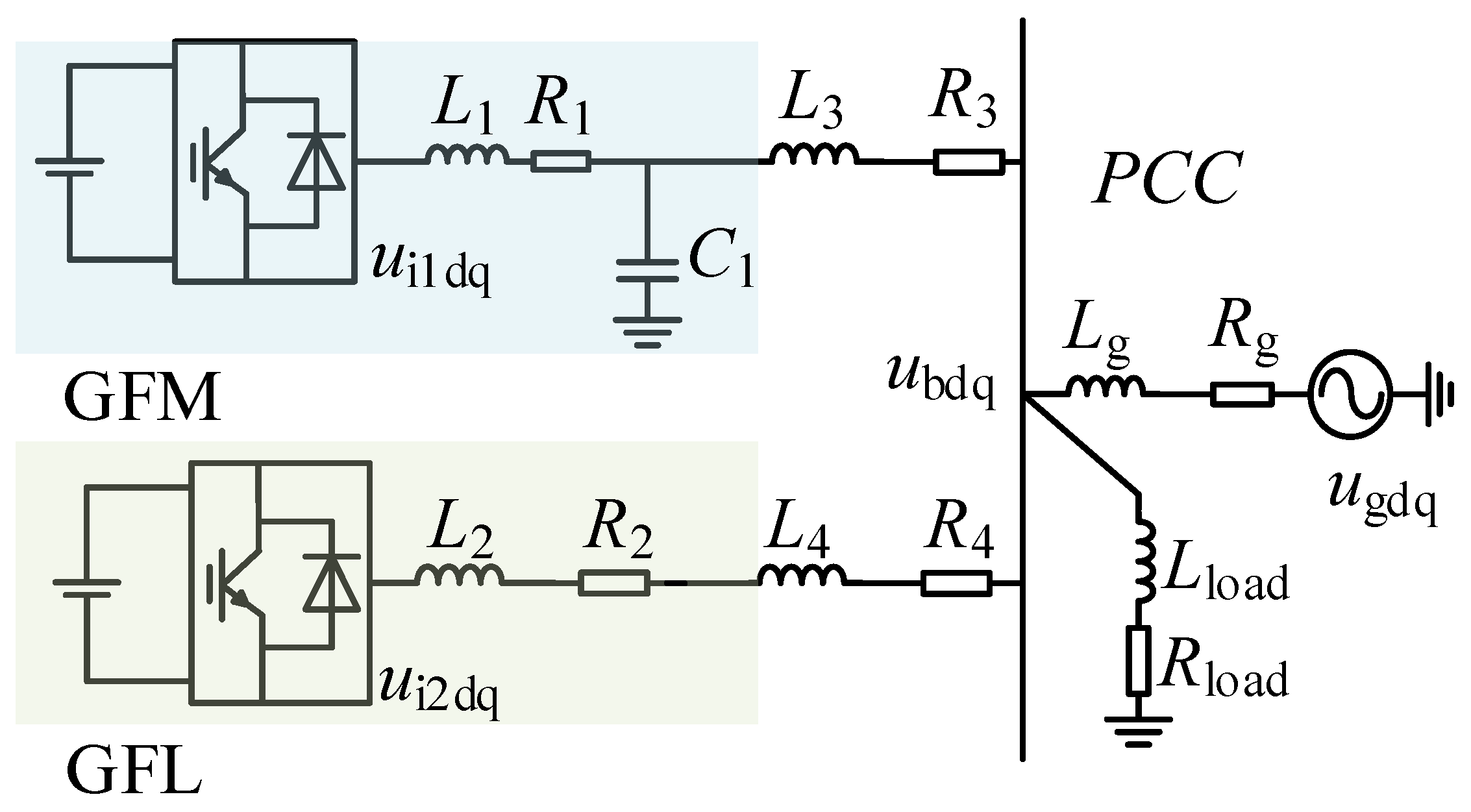
Figure 1. Heterogeneous Multi-Converter System.
Energies 19 04447 g001
Figure 2. Control Strategy of the GFM Converter.
Energies 19 04447 g002
Figure 3. Control Strategy of the GFL Converter.
Energies 19 04447 g003
Figure 4. Reference-Frame Transformation.
Energies 19 04447 g004
Figure 5. Eigenvalue trajectories as J varies.
Energies 19 04447 g005
Figure 6. Eigenvalue trajectories as Dp varies.
Energies 19 04447 g006
Figure 7. Eigenvalue trajectories as Kppll varies.
Energies 19 04447 g007
Figure 8. Eigenvalue trajectories as the SCR varies.
Energies 19 04447 g008
Figure 9. Stability heatmap for Dp and Kppll.
Energies 19 04447 g009
Figure 10. Stability heatmap for J and Kppll.
Energies 19 04447 g010
Figure 11. Output current of the GFM converter for J = 5, J = 0.5, and J = 0.1.
Energies 19 04447 g011
Figure 12. Output current of the GFL converter for Dp = 15, Dp = 2.5, and Dp = 1.
Energies 19 04447 g012
Figure 13. Output current of the GFL converter for Kppll = 0.8, Kppll = 2, and Kppll = 5.
Energies 19 04447 g013
Figure 14. PCC voltage waveforms of the system under simulation conditions 1 and 2, respectively.
Energies 19 04447 g014
Table 1. Interaction factors corresponding to the dominant modes at SCR = 1.5.
Dominant ModeOscillation FrequencyGFM ProportionGFL ProportionInteraction Factor
848.310.6040.5470.9507
1432.830.33540.62800.6963
1416.840.35960.63310.7244
167.700.66850.31600.6420
Table 3. Operating-condition parameters before and after optimization.
ConditionDpJKppll
Condition 130.52
Condition 2100.10.85
Disclaimer/Publisher’s Note: The statements, opinions and data contained in all publications are solely those of the individual author(s) and contributor(s) and not of MDPI and/or the editor(s). MDPI and/or the editor(s) disclaim responsibility for any injury to people or property resulting from any ideas, methods, instructions or products referred to in the content.