Impact of Grid-Following and Grid-Forming Inverter Integration on Bus Impedance Characteristics of Power Grids

Abstract

The increasing replacement of synchronous generators (SGs) by grid-following (GFL) and grid-forming (GFM) inverters is reshaping the dynamic bus characteristics of modern power systems. This transition makes a fixed ideal-voltage-source representation of the upstream main grid increasingly inadequate, especially when the interaction between inverter controls and network dynamics becomes significant. This paper investigates how the upstream grid bus admittance evolves with changes in source composition and observation location. An existing whole-system closed-loop impedance modeling framework is adopted. First, the parameter-dependent port characteristics of individual GFL and GFM inverters are analyzed to identify the frequency ranges dominated by external grid strength, synchronization mechanisms, and inner control loop dynamics. All frequencies reported herein are expressed in the synchronous $dq$ frame. Five representative scenarios are then constructed on the IEEE 16-machine 68-bus system to describe the transition from SG-dominated operation to GFL-rich and SG/GFL/GFM hybrid operation. The results show that increasing GFL penetration together with SG decommissioning does not cause a uniform change in bus admittance, but redistributes the low-frequency resonance characteristics among different locations. At 40% GFL penetration, disconnecting the corresponding SGs changes the dominant peak at electrically remote buses from 56.2 dB at 1.32 Hz to 66.0 dB at 2.44 Hz. When the GFL share is kept at 40% and 15% GFM capacity is introduced, the dominant low-frequency peaks decrease by 8.9 dB and 14.0 dB for buses close to generation sources and electrically remote buses, respectively, while the corresponding average low-frequency magnitude variations decrease by 20.6 dB and 14.7 dB. However, the dependence of bus admittance on network location remains evident. These results indicate that future transmission and distribution interface equivalents should account for source composition, observation location, and frequency dependence rather than relying solely on a fixed grid equivalent.

1. Introduction

The increasing penetration of renewable energy sources has been reshaping the dynamic characteristics of modern power systems [1]. In conventional power grids, synchronous generators (SGs) have long been the dominant devices responsible for voltage establishment, frequency regulation, inertial response, and short-circuit current contribution. Their electromechanical dynamics provide inherent inertia and damping, and their internal voltage behind transient reactance forms a relatively clear physical basis for the equivalent representation of the upstream grid. Therefore, when a distribution network is connected to a traditional transmission grid dominated by SGs, the upstream grid is often simplified as an ideal voltage source or a Thevenin equivalent source with a nearly fixed impedance [2]. This assumption is acceptable when the grid strength is sufficiently high and the dynamic interaction between the upstream grid and the downstream distribution system is relatively weak.

Unlike SGs, power-electronic converters do not naturally exhibit rotor inertia and electromagnetic synchronizing torque. Their external characteristics are mainly determined by control algorithms, current limitations, synchronization mechanisms, and inner-loop dynamics [3]. As a result, the equivalent behavior of the main grid seen from a distribution-network point of common coupling (PCC) is no longer determined only by network topology and synchronous reactance, but also by the control modes and capacity proportions of inverter-interfaced resources. In inverter-dominated systems, the upstream grid may exhibit frequency-dependent impedance, reduced damping, weaker voltage stiffness, and stronger coupling between active power, reactive power, voltage, and frequency [4]. These changes make the equivalent port characteristics of the main grid a key factor affecting the stability of connected distribution networks.

Among inverter-interfaced resources, grid-following (GFL) and grid-forming (GFM) inverters represent two typical control structures. A GFL inverter usually relies on a phase-locked loop (PLL) [5] or an equivalent synchronization unit to track the voltage phase of the PCC, and then injects controlled current according to the active and reactive power references. This control structure has been widely adopted in renewable generation plants because of its maturity and compatibility with conventional strong grids. Nevertheless, the operation of GFL inverters implicitly requires the presence of a sufficiently stiff external voltage reference. When the grid becomes weak, the interaction between the PLL, current control loop, and grid impedance may lead to oscillatory instability [6], poor damping, and even synchronization failure [7]. Therefore, a high proportion of GFL inverters may weaken the effective voltage support capability of the upstream grid and make its equivalent port behavior more sensitive to operating conditions and control parameters.

In contrast, GFM inverters are designed to establish or support the voltage and frequency at their terminals [8]. Instead of following an externally imposed voltage phase in the same manner as GFL inverters, GFM inverters can behave more like controlled voltage sources on the AC side [9]. Typical GFM implementations include droop control [10], virtual synchronous machine control [11], matching control [12], and other voltage-source-based synchronization mechanisms. These methods allow inverters to participate in voltage formation, frequency support, and power sharing. From the viewpoint of grid interaction, the presence of GFM inverters may increase the effective voltage stiffness and improve the small-signal stability of inverter-rich systems [13]. Nevertheless, GFM inverters are not ideal voltage sources. Their port characteristics are shaped by the outer power control, voltage loop, current loop, virtual impedance, current limitation, and the selected synchronization mechanism [14]. Therefore, the equivalent impedance or admittance contributed by GFM inverters is also frequency-dependent and may vary significantly with control parameters.

The distinction between GFL and GFM inverters has been extensively discussed in recent literature. Existing studies have shown that the difference between the two inverter types is not limited to whether a PLL is used. More fundamentally, it lies in their synchronization principles and port characteristics. GFL inverters can be regarded as voltage-following and current-forming devices, whereas GFM inverters can be regarded as current-following and voltage-forming devices from a duality perspective [15]. This theoretical interpretation indicates that the replacement of SGs by GFL or GFM inverters changes not only the amount of generation connected to the grid, but also the nature of the dynamic interface between the source side and the network side. Consequently, when GFL and GFM inverters coexist in the main grid, the bus impedance characteristics of power grids are determined by the combined effects of SGs, GFL inverters, GFM inverters, network impedances, and inverter control dynamics.

Impedance-based analysis provides a useful framework for studying inverter-grid interaction. By representing the upstream system through its equivalent impedance or admittance, the dynamic influence of different source compositions can be incorporated into distribution-network stability assessment. For example, when the upstream grid is dominated by SGs, the equivalent bus impedance may exhibit relatively passive and inductive characteristics over a broad frequency range. When GFM inverters are added, the voltage-source-like behavior may improve the low-frequency voltage support capability, but its virtual impedance and control-loop dynamics may also reshape the medium-frequency and high-frequency impedance characteristics. Therefore, the equivalent port of the main grid should be treated as a dynamic object rather than a fixed reactance.

Studies on GFL inverter stability have clarified that the stability of PLL-based inverters is strongly affected by grid impedance and grid strength. Under weak-grid conditions, the interaction between synchronization control and grid impedance may introduce negative damping [16] and cause low-frequency oscillations. Impedance reshaping, modified PLL structures, and adaptive control strategies have been proposed to extend the stable operating range of GFL inverters. These studies are highly relevant because they reveal that the main-grid equivalent impedance is not merely a passive background parameter; instead, it participates directly in the closed-loop dynamics of inverter-interfaced systems. For a distribution network connected to such an upstream grid, variations in the GFL proportion may therefore change not only the available active power, but also the dynamic boundary condition imposed at the PCC.

Some recent research has provided important insights into the role of GFM inverters in inverter-dominated power systems. Some studies have demonstrated that placing GFM inverters at appropriate locations can enhance the small-signal stability of systems with a large number of PLL-based inverters [17]. The underlying mechanism is often explained as an improvement in effective grid strength which is usually measured by short circuit ratio (SCR). Other studies have further investigated how the capacity ratio between GFM and GFL inverters affects small-signal stability and power grid strength [18]. More recently, some researchers have investigated the influence of GFM and GFL placement on the fundamental-frequency bus impedance of large power networks, and analyzed how the number and location of GFM inverters affect grid characteristics [19], whereas the evolution of wide-frequency bus admittance under changing SG/GFL/GFM compositions is not the primary concern. These works indicate that the proportion and placement of GFM inverters are closely related to the stability margin of inverter-rich systems. However, most of these studies are conducted from the viewpoint of transmission-level stability, inverter placement, or system-level grid strength. The equivalent port characteristics seen by a downstream distribution network are usually not the main focus.

As summarized in

Table 1. Comparison of existing studies and the present work.

Existing Work	Method	Main Focus	Objective	Difference from This Work
Song et al. [2]	Grid equivalent based on nodal U–I characteristics	Grid equivalent characteristics	Improve grid representation with power-electronic integration	Not focused on wide-frequency dynamic port characteristics
Yang et al. [17]	Small-signal analysis and generalized short-circuit ratio analysis	Grid strength and stability	Determine optimal GFM locations	Focuses on placement and stability rather than bus admittance evolution
Xin et al. [18]	Small-signal analysis with different GFM/GFL ratios	GFM proportion and stability margin	Determine the required GFM proportion	Focuses on stability requirements rather than bus admittance evolution
Yuan et al. [19]	Bus impedance analysis	Fundamental-frequency bus impedance	Assess GFM/GFL penetration and placement	Focuses on fundamental-frequency impedance rather than wide-frequency dynamics
Gu et al. [20]	Frame dynamics embedding and whole-system impedance modeling	System impedance, admittance, and modes	Enable impedance modeling of large composite AC systems	Provides the modeling method adopted here; SG/GFL/GFM composition evolution is not the main focus
This work	Whole-system closed-loop impedance modeling	Wide-frequency bus admittance	Track port changes during SG/GFL/GFM transition	—

, existing studies have addressed grid equivalent representation, whole-system impedance modeling, GFM placement, and the influence of GFM/GFL proportions from different perspectives. These studies provide important foundations for analyzing power-electronics-dominated grids. However, comparatively limited attention has been paid to how the wide-frequency bus admittance of an upstream multi-machine grid, as observed from distribution network access points, evolves as the generation structure changes from SG-dominated operation to GFL-rich and SG/GFL/GFM hybrid operation. In particular, the combined influence of source composition and observation location on the dynamic boundary presented by the upstream grid has not been the primary focus of previous studies. Therefore, this paper adopts the existing whole-system closed-loop impedance framework to investigate the evolution of upstream grid bus admittance under representative SG/GFL/GFM compositions and at different access locations in the IEEE 16-machine 68-bus system. The purpose is to provide a bus-level perspective on how the dynamic characteristics of the upstream grid change during this transition and to support more appropriate equivalent modeling of transmission and distribution interfaces.

The remainder of this paper is organized as follows. Section 2 presents the impedance-based characteristic analysis of GFL and GFM inverters under variations in key control and system parameters. This section focuses on the single-inverter condition and clarifies how different control parameters affect inverter dynamics in different frequency ranges. Section 3 introduces the whole-system closed-loop impedance modeling method adopted in this paper, which is developed based on existing studies, and describes the simulation scenario design using the IEEE 16-machine 68-bus system. Section 4 presents and discusses the simulation results under different source-composition scenarios. Finally, Section 5 summarizes the main conclusions of this paper.

2. Impedance-Based Characteristic Analysis of GFL and GFM Inverters

2.1. GFL Inverter

2.1.1. Topology and Control Method

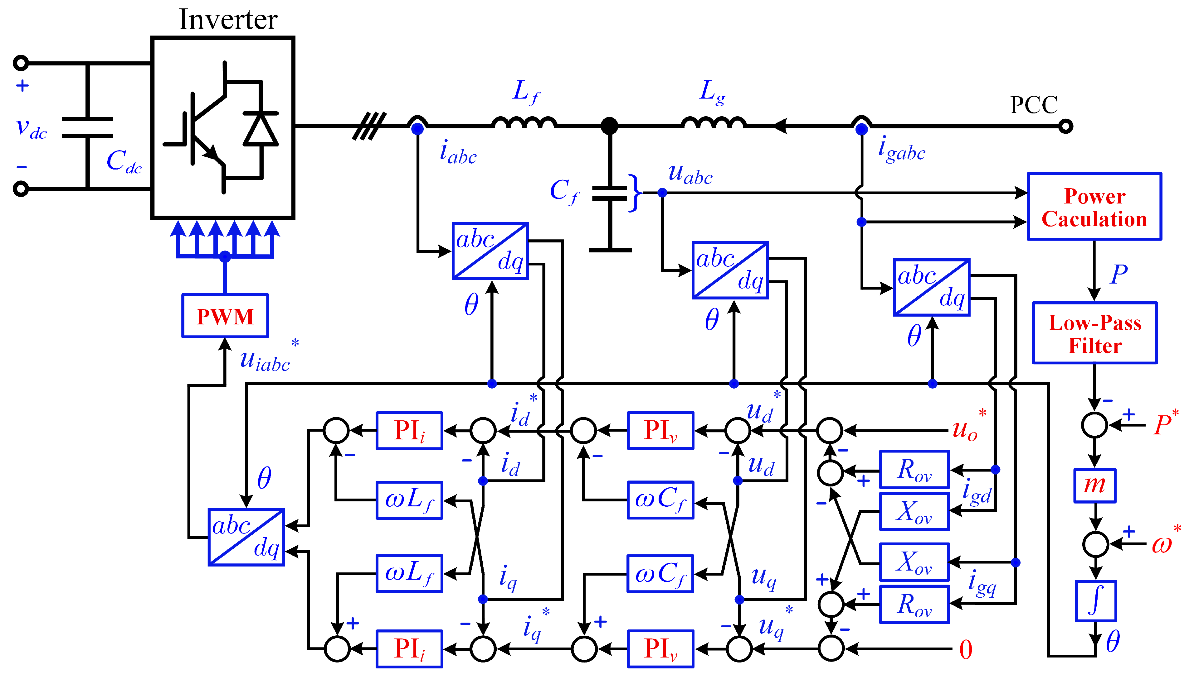
In the GFL inverter considered in this section, the AC-side interface is composed of an inverter and an output filter connected to the PCC. The control block diagram is shown in Figure 1. Depending on the filtering requirement, an LC or LCL filter can be adopted to attenuate the switching-frequency components before the inverter is connected to the external network. The measured three-phase output voltages and currents are transformed into the synchronous ($dq$) reference frame for control implementation. The reference-frame angle is obtained from the PCC voltage by a PLL, so that the d-axis component is aligned with the grid voltage vector under steady-state conditions. In this case, the q-axis voltage component is close to zero. Therefore, the active and reactive power can be regulated primarily through the d- and q-axis current components, respectively.

The control system is usually organized in a cascaded structure. The outer control loop generates the current references according to the active power, reactive power, DC-voltage, or power factor commands, while the inner current loop regulates the filter current in the synchronous reference frame. In practical implementation, proportional-integral regulators are commonly used in the current loop. Cross-coupling compensation terms and grid-voltage feedforward are introduced to improve the current tracking performance and to reduce the coupling between the d- and q-axis dynamics. The voltage commands generated by the current controller are then transformed back to the three-phase stationary ($abc$) frame and sent to the pulse-width modulation (PWM) unit to produce the switching signals of the inverter.

This control structure is mature and has been widely applied because of its clear physical interpretation and convenient independent regulation of active and reactive power under balanced grid conditions. Nevertheless, its small-signal behavior at the grid-connected port is jointly shaped by the PLL, the current controller, the filter parameters, and the operating point. Variations in these parameters may significantly change the terminal impedance characteristics of the GFL inverter. Therefore, before analyzing the equivalent bus characteristics of a larger network, it is necessary to clarify how the key parameters of a single GFL inverter affect its impedance spectrum. This provides the basis for the advanced analysis carried out in the following section.

2.1.2. Impedance Characteristic Analysis

In this paper, the port or bus characteristics are described in the admittance form. This choice is consistent with the nodal representation of power networks, where transmission lines, transformers, shunt branches, loads, compensation devices, and converter terminals can be naturally assembled into the network admittance matrix. For a multi-bus system, the nodal equation is generally written as

$$I=Y_{bus}V.$$

(1)

Therefore, when a voltage perturbation is applied at a selected bus, the corresponding current response can be directly used to characterize the local bus admittance as

$$Y\left(s\right)={\displaystyle \frac{\Delta I\left(s\right)}{\Delta V\left(s\right)}}.$$

(2)

This form is also consistent with the small-signal modeling of grid-connected inverters, where the terminal voltage perturbation is usually taken as the input and the current response is taken as the output.

For three-phase systems, the measured perturbation variables are transformed into the synchronous ($dq$) reference frame. The bus admittance is then represented as a multi-input multi-output matrix:

$$\left[\begin{array}{c}\Delta I_d\\ \Delta I_q\end{array}\right]=\left[\begin{array}{cc}{Y}_{dd}& Y_{dq}\\ Y_{qd}& Y_{qq}\end{array}\right]\left[\begin{array}{c}\Delta V_d\\ \Delta V_q\end{array}\right].$$

(3)

In this study, all small-signal terminal variables are expressed in a common steady synchronous reference frame rotating at the fundamental angular frequency ${\omega }_0$. The d axis is aligned with the steady-state voltage vector at the reference bus. For a positive-sequence perturbation with angular frequency ${\omega }_p$ in the stationary frame, the corresponding frequency observed in the synchronous frame is $\omega ={\omega }_p-{\omega }_0$. Therefore, the frequency variable used in the following $dq$ domain responses represents the perturbation frequency relative to the synchronous fundamental frequency.

The full $dq$ admittance model in (3) is retained as a $2\times 2$ MIMO representation. By applying the complex sequence transformation, it can be written in the positive and negative sequence form as

$$\left[\begin{array}{c}\Delta I_{+}\\ \Delta I_{-}\end{array}\right]=\left[\begin{array}{cc}{Y}_{++}& Y_{+-}\\ Y_{-+}& Y_{--}\end{array}\right]\left[\begin{array}{c}\Delta V_{+}\\ \Delta V_{-}\end{array}\right],$$

(4)

where $Y_{++}$ and $Y_{--}$ represent the positive and negative sequence self admittances, respectively, while $Y_{+-}$ and $Y_{-+}$ describe the coupling between the two sequence components.

To obtain the sequence-domain characteristic, the ($dq$)-frame admittance matrix is further transformed, and the positive-sequence self admittance used for the frequency response comparison in this paper is

$$Y_{\mathrm{dq}+}\left(s\right)\equiv Y_{++}\left(s\right)={\displaystyle \frac{Y_{dd}\left(s\right)+Y_{qq}\left(s\right)}{2}}+j{\displaystyle \frac{Y_{qd}\left(s\right)-Y_{dq}\left(s\right)}{2}}.$$

(5)

The scalar quantity $Y_{\mathrm{dq}+}=Y_{++}$ is used here to characterize the positive-sequence bus admittance under the balanced three-phase, symmetric steady state, and small-signal operating conditions considered in this study. Under these assumptions, the positive-sequence response is selected as the principal quantity for comparing different buses and source composition scenarios. It should be emphasized that this does not replace the full matrix formulation used in the whole-system model. The complete $dq$ or sequence-domain matrices are retained during system interconnection, while $Y_{++}$ is extracted only for presenting the positive-sequence frequency response. The off-diagonal terms $Y_{+-}$ and $Y_{-+}$ represent the mirror-frequency coupling between positive and negative sequence components. When these coupling terms become significant, the scalar $Y_{++}$ alone is insufficient to characterize the complete port dynamics, and the full matrix formulation should be retained.

The dynamic equations of the GFL inverter used in this study are summarized below. The PLL is synchronized with the PCC voltage, with the d axis aligned with the steady-state grid voltage. Its dynamics are expressed as

$$\left\{\begin{array}{cc}\hfill {\dot{\varphi }}_{uq}\hfill & =u_q^{*}-u_q,\hfill \\ \hfill \omega \hfill & ={\omega }_g+k_{p,pll}\left(u_q^{*}-u_q\right)+k_{i,pll}{\varphi }_{uq},\hfill \\ \hfill \dot{\delta }\hfill & =\omega -{\omega }_g,\hfill \end{array}\right.$$

(6)

where $u_q^{*}=0$ under the adopted voltage-oriented synchronization, ${\varphi }_{uq}$ is the PLL integral state, $\omega$ is the estimated angular frequency, ${\omega }_g$ is the grid angular frequency, and $\delta$ is the angular displacement between the local PLL frame and the grid reference frame.

The inner current controller is described by

$$\left\{\begin{array}{cc}\hfill {\dot{\varphi }}_{id}\hfill & =i_d^{*}-i_d,\hfill \\ \hfill {\dot{\varphi }}_{iq}\hfill & =i_q^{*}-i_q,\hfill \\ \hfill e_d\hfill & =k_{pi}\left(i_d^{*}-i_d\right)+k_{ii}{\varphi }_{id}-\omega L_f{i}_q,\hfill \\ \hfill e_q\hfill & =k_{pi}\left(i_q^{*}-i_q\right)+k_{ii}{\varphi }_{iq}+\omega L_f{i}_d,\hfill \end{array}\right.$$

(7)

where $i_d^{*}$ and $i_q^{*}$ are the current references, ${\varphi }_{id}$ and ${\varphi }_{iq}$ are the current controller integral states, and $e_d$ and $e_q$ are the inverter-side voltage outputs.

The LC filter and grid connection dynamics in the local synchronous reference frame are given by

$$\left\{\begin{array}{cc}\hfill {\dot{i}}_d\hfill & ={\displaystyle \frac{1}{L_f}}\left(e_d-u_d+\omega L_f{i}_q-R_f{i}_d\right),\hfill \\ \hfill {\dot{i}}_q\hfill & ={\displaystyle \frac{1}{L_f}}\left(e_q-u_q-\omega L_f{i}_d-R_f{i}_q\right),\hfill \\ \hfill {\dot{u}}_d\hfill & ={\displaystyle \frac{1}{C_f}}\left(i_d-i_{gd}+\omega C_f{u}_q\right),\hfill \\ \hfill {\dot{u}}_q\hfill & ={\displaystyle \frac{1}{C_f}}\left(i_q-i_{gq}-\omega C_f{u}_d\right),\hfill \\ \hfill {\dot{i}}_{gd}\hfill & ={\displaystyle \frac{1}{L_g}}\left(u_d-u_{gd}+\omega L_g{i}_{gq}-R_g{i}_{gd}\right),\hfill \\ \hfill {\dot{i}}_{gq}\hfill & ={\displaystyle \frac{1}{L_g}}\left(u_q-u_{gq}-\omega L_g{i}_{gd}-R_g{i}_{gq}\right).\hfill \end{array}\right.$$

(8)

Accordingly, the GFL dynamic state vector can be written as

$${\mathbf{x}}_{\mathrm{GFL}}={\left[\delta ,{\varphi }_{uq},{\varphi }_{id},{\varphi }_{iq},i_d,i_q,u_d,u_q,i_{gd},i_{gq}\right]}^{\mathrm{T}}.$$

(9)

Based on the above dynamic equations, the GFL model is linearized around its steady-state operating point. The main parameters of the GFL inverter model are listed in

Table 2. Main parameters of the GFL inverter model.

Parameter	Value	Parameter	Value
Base voltage $V_{\mathrm{base}}$	200 V	Filter reactance ${\omega }_0{L}_f$	0.05 pu
Base power $S_{\mathrm{base}}$	10 kVA	Filter resistance $R_f$	0.01 pu
Base frequency $f_{\mathrm{base}}$	50 Hz	Filter susceptance ${\omega }_0{C}_f$	0.02 pu
Active power output P	0.6 pu	Grid-side reactance ${\omega }_0{L}_g$	0.10 pu
Reactive power output Q	0.1 pu	Grid-side resistance $R_g$	0.02 pu
PLL bandwidth $f_{pll}$	10 Hz	Current-loop bandwidth ${\omega }_i$	$800·2\pi$ rad/s
PLL proportional gain $k_{p,pll}$	$f_{pll}·2\pi$	Current-loop proportional gain $k_{pi}$	$L_f·{\omega }_i$
PLL integral gain $k_{i,pll}$	$k_{p,pll}^2/4$	Current-loop integral gain $k_{ii}$	$L_f·{\omega }_i^2/4$

. The PCC voltage perturbation $\Delta u_{g,dq}={[\Delta u_{gd},\Delta u_{gq}]}^{\mathrm{T}}$ is selected as the external input, and the grid-side current perturbation $\Delta i_{g,dq}={[\Delta i_{gd},\Delta i_{gq}]}^{\mathrm{T}}$ is selected as the output. By eliminating the internal state perturbations, the small-signal terminal relation can be expressed as

$$\Delta i_{g,dq}\left(s\right)=Y_{\mathrm{GFL},dq}\left(s\right)\Delta u_{g,dq}\left(s\right),$$

(10)

where $Y_{\mathrm{GFL},dq}\left(s\right)$ is the $2\times 2$ terminal admittance matrix in the local reference frame. The corresponding impedance matrix is obtained as

$$Z_{\mathrm{GFL},dq}\left(s\right)=Y_{\mathrm{GFL},dq}^{-1}\left(s\right).$$

(11)

The local impedance model is subsequently transformed to obtain the device impedance $Z_m\left(s\right)$ used in the whole-system model described in Section 3.1.

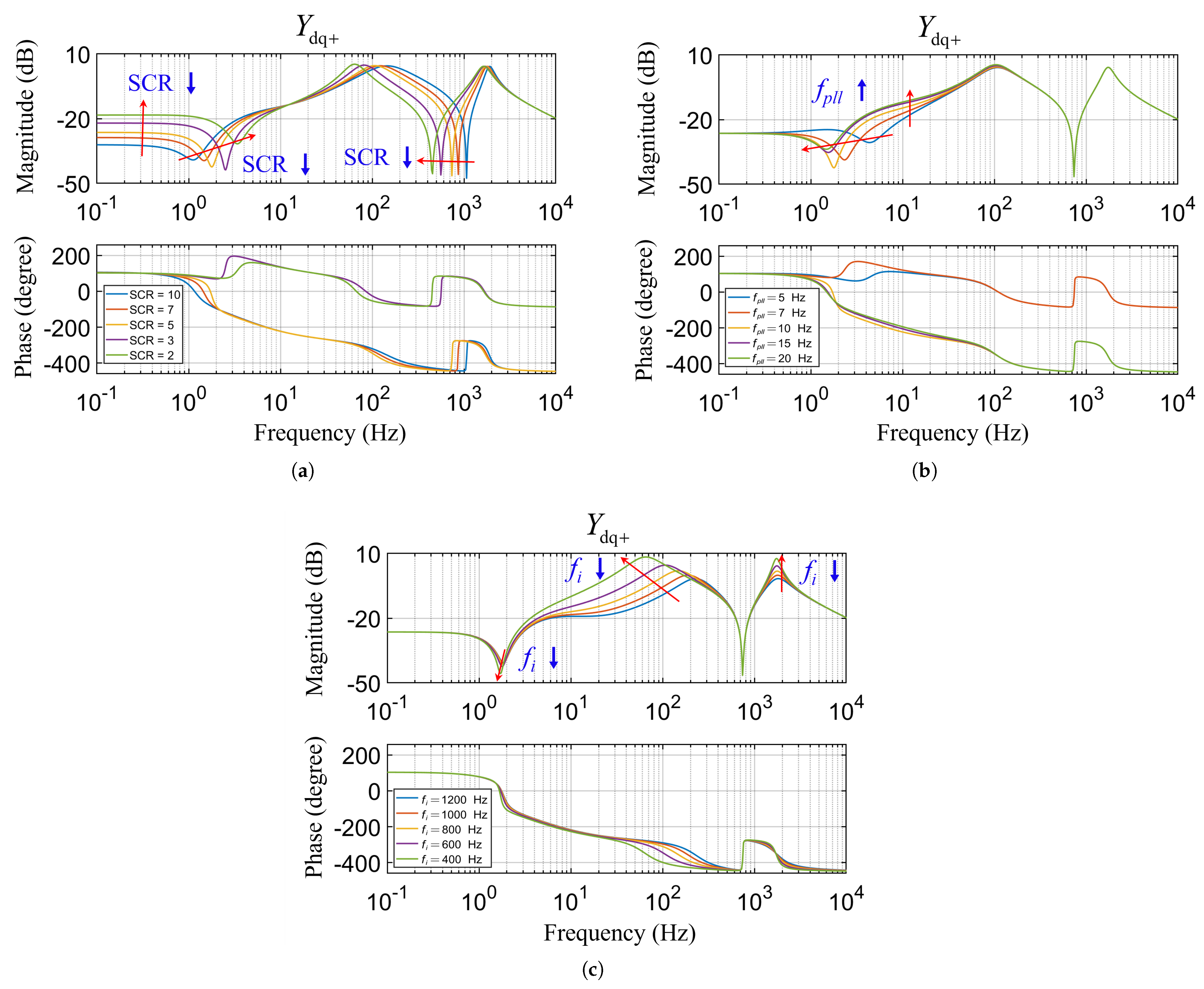
Figure 2 shows the variation of the positive-sequence bus admittance $Y_{\mathrm{dq}+}$ of the GFL inverter under different grid strengths, PLL bandwidths $f_{pll}$, and current-loop bandwidths $f_i$. The grid strength in the single-inverter infinite-bus system is characterized by SCR, defined as

$$\mathrm{SCR}={\displaystyle \frac{S_{\mathrm{sc}}}{S_n}}={\displaystyle \frac{V_{\mathrm{PCC}}^2}{|Z_{\mathrm{grid}}|S_n}},$$

(12)

where $S_{\mathrm{sc}}$ is the short-circuit capacity at the PCC, $S_n$ is the rated capacity of the inverter, and $Z_{\mathrm{grid}}=R_{\mathrm{grid}}+j{X}_{\mathrm{grid}}$ is the equivalent impedance between the PCC and the infinite bus. With $S_{\mathrm{base}}=S_n$ and $V_{\mathrm{PCC}}=V_{\mathrm{base}}$, the SCR in per-unit form becomes

$$\mathrm{SCR}={\displaystyle \frac{1}{|Z_{\mathrm{grid},\mathrm{pu}}|}}={\displaystyle \frac{1}{\sqrt{R_{\mathrm{grid},\mathrm{pu}}^2+X_{\mathrm{grid},\mathrm{pu}}^2}}}.$$

(13)

In Figure 2a, the decrease in SCR leads to a clear increase in the low-frequency admittance magnitude. Since admittance represents the current response caused by a terminal voltage perturbation, this result indicates that the inverter terminal becomes more sensitive to voltage disturbances when the external grid is weakened. Meanwhile, the valley and peak characteristics in the low-frequency range become more pronounced as SCR decreases, and the phase curve also exhibits a larger deviation. This shows that the external grid impedance is not only a passive series element, but also participates in the closed-loop dynamics through its interaction with the PLL and current controller. In addition, the resonance and notch characteristics in the middle- and high-frequency ranges also vary with SCR, implying that the external network condition can reshape the bus admittance over a relatively wide frequency range rather than only changing the fundamental-frequency short-circuit level.

The influence of the PLL bandwidth $f_{pll}$ is mainly concentrated in the low-frequency range, as shown in Figure 2b. When $f_{pll}$ increases, the frequency band affected by the synchronization loop moves toward higher frequencies, and the magnitude variation around this band becomes more evident. The corresponding phase response also changes significantly, which means that the PLL modifies both the amplitude and phase of the terminal admittance associated with synchronization dynamics. However, the admittance curves in the lower-frequency range remain almost unchanged, indicating that the PLL has limited influence on the dynamics dominated by the filter and current loop. Therefore, the PLL bandwidth primarily determines how the inverter responds to slow voltage-angle and frequency perturbations at the grid-connected port.

Figure 2c presents the effect of the current-loop bandwidth $f_i$. Compared with SCR and PLL bandwidth, $f_i$ mainly affects the middle-frequency range. As $f_i$ decreases, the admittance magnitude increases in the region of tens to hundreds of hertz, and the main peak shifts toward a lower frequency. At the same time, the phase roll-off also appears earlier, reflecting the reduced response speed of the current loop. This indicates that the current controller directly shapes the dynamic current response of the inverter terminal in the frequency band close to its control bandwidth, while its influence on the very low-frequency synchronization-dominated region is relatively limited.

Overall, these results show that different factors modify different parts of the GFL terminal admittance spectrum. The grid strength affects the interaction between the inverter and the external network; the PLL bandwidth reshapes the low-frequency synchronization-related admittance; and the current-loop bandwidth mainly determines the middle-frequency current-response characteristics. Therefore, the port characteristic of a GFL inverter is not a fixed passive impedance, but a frequency-dependent dynamic admittance determined jointly by the external grid and the control system. This observation provides an important basis for the following analysis of how the connection of SGs, GFL inverters, and GFM inverters changes the bus characteristics of the main grid.

2.2. GFM Inverter

2.2.1. Topology and Control Method

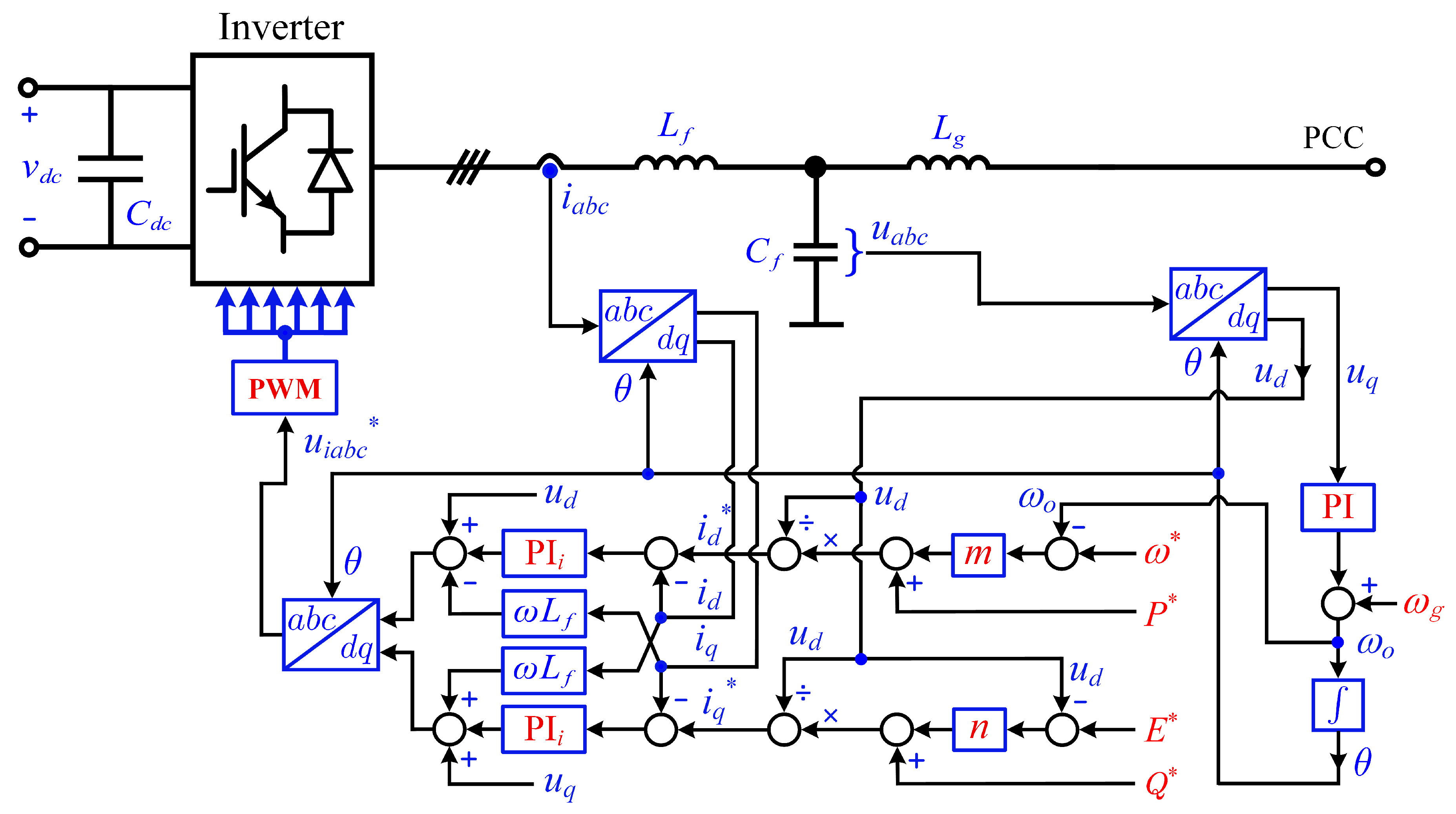
The GFM inverter studied in this section consists of a three-phase inverter, an LC filter, and a grid-side connection to the PCC. The control block diagram is shown in Figure 3. The capacitor voltage and grid-side current are measured for power calculation and feedback control. The instantaneous active power is filtered and then used in the power–frequency droop loop, from which the angular frequency is obtained and integrated to generate the internal synchronous angle for the ($abc/dq$) transformations.

In the control system, the capacitor voltage is transformed into the internally defined ($dq$) frame and regulated by the voltage loop, whose output provides the current reference for the inner current loop. A virtual impedance loop is introduced in the voltage reference path, where the grid-side current is fed back through virtual resistance and reactance terms. This enables the terminal voltage command to vary with the output current and reshapes the inverter port characteristic without changing the physical filter parameters. The inner current loop then generates the modulation voltage command, which is transformed back to the three-phase frame and applied to the PWM module. For both the GFL and GFM inverter models, the DC side is represented by an ideal stiff voltage source with a constant voltage $V_{\mathrm{dc}}$. Control computation, sampling, and modulation delays are neglected in the small-signal models. In addition, no current limiting or saturation is included, and the inverters are assumed to operate within their linear control and modulation ranges. These assumptions are adopted because the present study focuses on the small-signal bus admittance characteristics around the specified steady-state operating points. Therefore, the bus admittance of the GFM inverter is jointly affected by the droop coefficient, droop-control bandwidth, voltage loop, current loop, virtual impedance, etc., which provides the basis for the following impedance-spectrum analysis.

2.2.2. Impedance Characteristic Analysis

The dynamic model of the GFM inverter consists of the power-frequency synchronization loop, virtual impedance, cascaded voltage and current controllers, and the LC filter dynamics. Unlike the GFL inverter, whose local reference frame is generated by the PLL, the GFM inverter establishes its own internal angle through the power-frequency control loop. Therefore, the active power dynamics directly participate in the formation of the local synchronous reference frame. The instantaneous active and reactive power measured at the grid side are calculated as

$$\left\{\begin{array}{cc}\hfill p\hfill & =u_{gd}{i}_{gd}+u_{gq}{i}_{gq},\hfill \\ \hfill q\hfill & =u_{gq}{i}_{gd}-u_{gd}{i}_{gq}.\hfill \end{array}\right.$$

(14)

The active power is used as the feedback signal of the power-frequency synchronization loop. A first-order low-pass filter is incorporated into the droop control. The resulting angular frequency determines the rotational speed of the internally generated reference frame, while its deviation from the grid frequency produces the relative angle dynamics. Accordingly, the active power droop dynamics are represented by

$$\left\{\begin{array}{cc}\hfill \dot{\omega }& ={\omega }_f\left[m_p\left(p^{*}-p\right)+\left({\omega }^{*}-\omega \right)\right],\hfill \\ \hfill \dot{\delta }& =\omega -{\omega }_g,\hfill \end{array}\right.$$

(15)

where ${\omega }_f$ is the droop control bandwidth, $m_p$ is the active power droop coefficient, $p^{*}$ is the active power reference, and $\delta$ denotes the angular displacement between the internally generated GFM reference frame and the grid reference frame.

In addition, a virtual impedance is also introduced to reshape the terminal voltage-current relationship without modifying the physical filter parameters. The grid-side current is fed back through the virtual resistance and reactance, to modify the voltage reference seen by the outer voltage controller. The modified voltage references are expressed as

$$\left\{\begin{array}{cc}\hfill u_d^{*}\hfill & =u_o^{*}+R_{ov}{i}_{gd}-X_{ov}{i}_{gq},\hfill \\ \hfill u_q^{*}\hfill & =R_{ov}{i}_{gq}+X_{ov}{i}_{gd},\hfill \end{array}\right.$$

(16)

where $R_{ov}$ and $X_{ov}$ denote the virtual resistance and virtual reactance, respectively.

The voltage and current regulation loops adopt a cascaded control structure. The outer voltage controller regulates the filter capacitor voltage and generates the references $i_d^{*}$ and $i_q^{*}$ for the inner current controller. The corresponding integral states are denoted by ${\varphi }_{ud}$ and ${\varphi }_{uq}$. The inner current loop then regulates the inverter-side inductor currents and generates the inverter voltage commands $e_d$ and $e_q$, with ${\varphi }_{id}$ and ${\varphi }_{iq}$ representing the associated integral states. The cross-coupling terms introduced by the synchronous $dq$ transformation are compensated in both control loops. Accordingly, the cascaded voltage and current control dynamics are expressed as

$$\left\{\begin{array}{cc}\hfill {\dot{\varphi }}_{ud}\hfill & =u_d^{*}-u_d,\hfill \\ \hfill {\dot{\varphi }}_{uq}\hfill & =u_q^{*}-u_q,\hfill \\ \hfill i_d^{*}\hfill & =k_{pv}\left(u_d^{*}-u_d\right)+k_{iv}{\varphi }_{ud}-\omega C_f{u}_q,\hfill \\ \hfill i_q^{*}\hfill & =k_{pv}\left(u_q^{*}-u_q\right)+k_{iv}{\varphi }_{uq}+\omega C_f{u}_d,\hfill \\ \hfill {\dot{\varphi }}_{id}\hfill & =i_d^{*}-i_d,\hfill \\ \hfill {\dot{\varphi }}_{iq}\hfill & =i_q^{*}-i_q,\hfill \\ \hfill e_d\hfill & =k_{pi}\left(i_d^{*}-i_d\right)+k_{ii}{\varphi }_{id}-\omega L_f{i}_q,\hfill \\ \hfill e_q\hfill & =k_{pi}\left(i_q^{*}-i_q\right)+k_{ii}{\varphi }_{iq}+\omega L_f{i}_d.\hfill \end{array}\right.$$

(17)

The LC filter and grid connection dynamics are

$$\left\{\begin{array}{cc}\hfill {\dot{i}}_d\hfill & ={\displaystyle \frac{1}{L_f}}\left(e_d-u_d+\omega L_f{i}_q-R_f{i}_d\right),\hfill \\ \hfill {\dot{i}}_q\hfill & ={\displaystyle \frac{1}{L_f}}\left(e_q-u_q-\omega L_f{i}_d-R_f{i}_q\right),\hfill \\ \hfill {\dot{u}}_d\hfill & ={\displaystyle \frac{1}{C_f}}\left(i_d-i_{gd}+\omega C_f{u}_q\right),\hfill \\ \hfill {\dot{u}}_q\hfill & ={\displaystyle \frac{1}{C_f}}\left(i_q-i_{gq}-\omega C_f{u}_d\right),\hfill \\ \hfill {\dot{i}}_{gd}\hfill & ={\displaystyle \frac{1}{L_g}}\left(u_d-u_{gd}+\omega L_g{i}_{gq}-R_g{i}_{gd}\right),\hfill \\ \hfill {\dot{i}}_{gq}\hfill & ={\displaystyle \frac{1}{L_g}}\left(u_q-u_{gq}-\omega L_g{i}_{gd}-R_g{i}_{gq}\right).\hfill \end{array}\right.$$

(18)

Accordingly, the GFM dynamic state vector is expressed as

$${\mathbf{x}}_{\mathrm{GFM}}={\left[\omega ,\delta ,{\varphi }_{ud},{\varphi }_{uq},{\varphi }_{id},{\varphi }_{iq},i_d,i_q,u_d,u_q,i_{gd},i_{gq}\right]}^{\mathrm{T}}.$$

(19)

Similarly, the GFM dynamic equations are linearized around the corresponding steady-state operating point. The main parameters of the GFM inverter model are listed in

Table 3. Main parameters of the GFM inverter model.

Parameter	Value	Parameter	Value
Base voltage $V_{\mathrm{base}}$	200 V	Grid-side reactance ${\omega }_0{L}_g$	0.10 pu
Base power $S_{\mathrm{base}}$	10 kVA	Grid-side resistance $R_g$	0.02 pu
Base frequency $f_{\mathrm{base}}$	50 Hz	Current-loop bandwidth ${\omega }_i$	$1000·2\pi$ rad/s
Active power output P	0.6 pu	Current-loop proportional gain $k_{pi}$	$L_f·{\omega }_i$
Reactive power output Q	0.1 pu	Current-loop integral gain $k_{ii}$	$L_f·{\omega }_i^2/4$
Droop-control bandwidth ${\omega }_f$	$5·2\pi$ rad/s	Voltage-loop bandwidth ${\omega }_v$	$400·2\pi$ rad/s
Droop coefficient $m_p$	0.05 pu	Voltage-loop proportional gain $k_{pv}$	$C_f·{\omega }_v$
Filter reactance ${\omega }_0{L}_f$	0.05 pu	Voltage-loop integral gain $k_{iv}$	$20C_f·{\omega }_v^2/4$
Filter resistance $R_f$	0.01 pu	Virtual resistance $R_{ov}$	0.10 pu
Filter susceptance ${\omega }_0{C}_f$	0.02 pu	Virtual reactance $X_{ov}$	0.02 pu

.

The PCC voltage perturbation $\Delta u_{g,dq}={[\Delta u_{gd},\Delta u_{gq}]}^{\mathrm{T}}$ and the grid-side current perturbation $\Delta i_{g,dq}={[\Delta i_{gd},\Delta i_{gq}]}^{\mathrm{T}}$ are selected as the terminal variables. Eliminating the internal state perturbations gives

$$\Delta i_{g,dq}\left(s\right)=Y_{\mathrm{GFM},dq}\left(s\right)\Delta u_{g,dq}\left(s\right),$$

(20)

and the corresponding terminal impedance is

$$Z_{\mathrm{GFM},dq}\left(s\right)=Y_{\mathrm{GFM},dq}^{-1}\left(s\right).$$

(21)

The frame dynamics associated with the internally generated GFM angle are then embedded into the local impedance model according to the transformation introduced in Section 3.1, yielding the device impedance $Z_m\left(s\right)$ for whole-system interconnection.

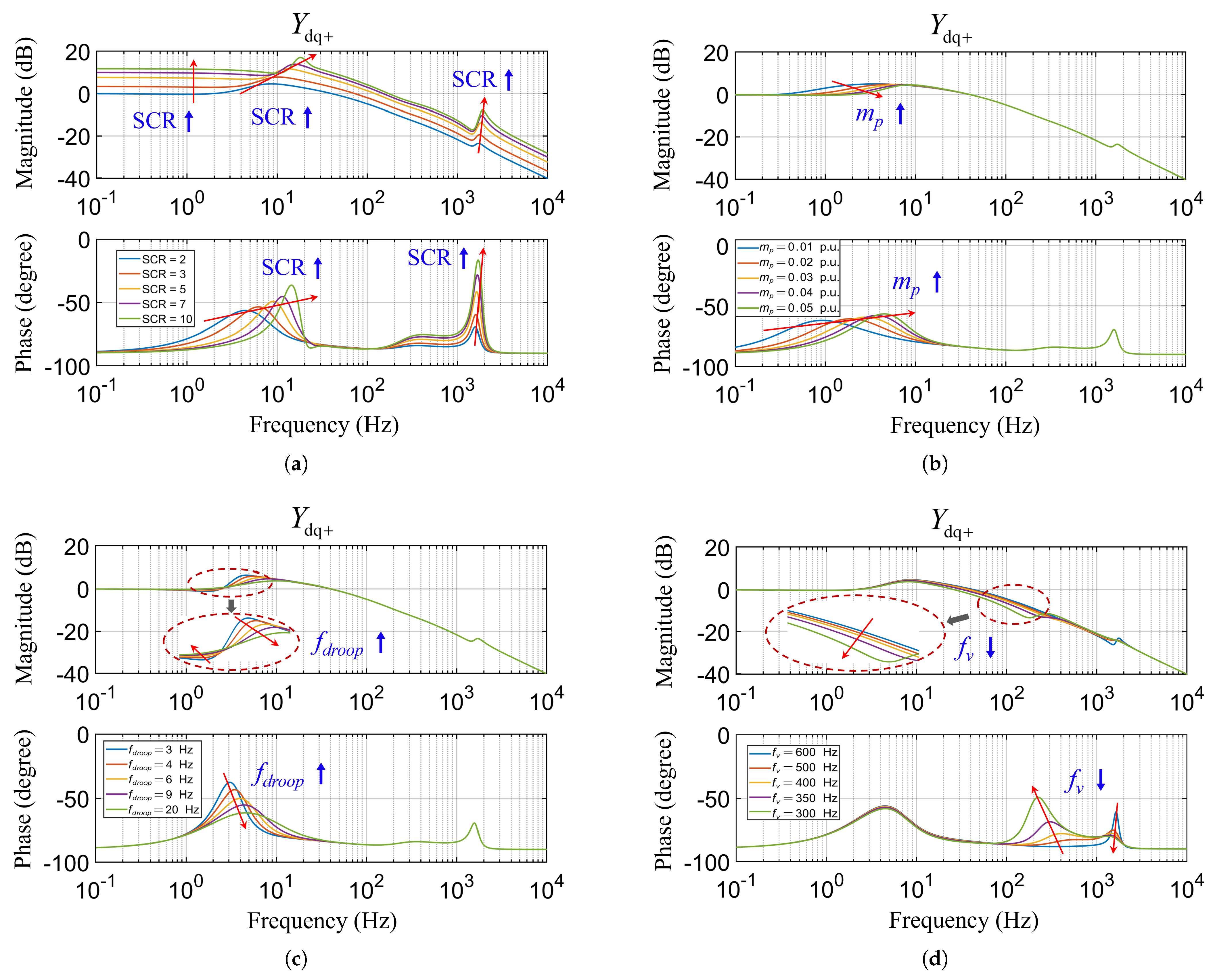
Figure 4 illustrates the influence of SCR, droop coefficient $m_p$, droop-control bandwidth $f_{droop}$, and voltage-loop bandwidth $f_v$ on the positive-sequence admittance $Y_{\mathrm{dq}+}$ of the GFM inverter. As shown in Figure 4a, as SCR increases, the low-frequency magnitude of $Y_{\mathrm{dq}+}$ increases noticeably, and the characteristic peak in the several-hertz to tens-of-hertz range moves to a higher frequency. This indicates that a stronger external grid changes the terminal voltage-current relationship by modifying the interaction condition between the inverter and the network.

Figure 4b shows that the variation of $m_p$ mainly affects the low-frequency region, while its influence on the middle- and high-frequency characteristics is relatively limited. In this model, the virtual inertia and damping are related to the droop parameters. Therefore, increasing $m_p$ reduces the equivalent virtual inertia and damping simultaneously. As a result, the low-frequency admittance associated with the power-frequency regulation loop is slightly reshaped, especially in the phase response. However, since the voltage loop, current loop, and filter parameters remain unchanged, the high-frequency part of $Y_{\mathrm{dq}+}$ is almost unaffected.

The effect of $f_{droop}$ is presented in Figure 4c. In contrast to the effect of $m_p$, changing $f_{droop}$ directly changes the dynamic range of the power-measurement and droop-control loop. When $f_{droop}$ increases, the admittance variation related to the droop loop extends toward a higher frequency range, and both the magnitude and phase curves in the low-frequency band move accordingly. This means that the bandwidth of the droop-control loop determines how fast the inverter frequency responds to power disturbances, and thus reshapes the low-frequency bus admittance.

Figure 4d further shows that the voltage-loop bandwidth $f_v$ mainly influences the middle-frequency range. As $f_v$ decreases, the voltage regulation dynamics become slower, and the corresponding magnitude and phase transitions move toward lower frequencies. Meanwhile, the low-frequency droop-dominated part changes very slightly, indicating that $f_v$ mainly determines the voltage-control-related admittance rather than the power-synchronization behavior.

Overall, SCR, droop coefficient $m_p$, droop-control bandwidth $f_{droop}$, and voltage-loop bandwidth $f_v$ affect different regions of the GFM admittance spectrum. The results reveal that the port characteristic of a GFM inverter is jointly determined by the external grid condition, power-synchronization loop, voltage regulation loop, and filter dynamics, which provides a basis for analyzing how GFM inverters reshape the bus characteristics of the main grid.

3. Method and Simulation Design

In conventional impedance-based modeling of power systems, the system under study is typically partitioned into a “source side” and a “load side”. The corresponding source-side and load-side impedance models are then established separately, and the small-signal stability is assessed at the PCC using impedance-ratio-based criteria [21]. Owing to its clear physical interpretation and relatively simple structure, this approach has been widely used for stability analysis of single-inverter grid connection, weak-grid interactions, and single-machine infinite-bus systems. In such applications, the system boundary can usually be clearly defined, and the interaction between the device and the external network can be characterized by the impedance relationship observed at a selected interface.

However, when the study object is extended to a complex system consisting of SGs, GFL inverters, GFM inverters, and dynamic loads, the traditional source-load partitioning becomes less straightforward [22]. First, the boundary between sources, loads, and network components is no longer unique in meshed networks and multi-device systems. Some apparatus may exhibit both source-like and load-like dynamic characteristics, and the oscillatory behavior of the system is often determined by the closed-loop interaction of all devices through the network rather than by a local impedance interaction at a single interface. If SGs, GFL inverters, GFM inverters, and flexible devices are all placed on the “device side” independently, the coupling among device dynamics, network topology, and other devices may be partially neglected. Second, the dynamic reference frames of different devices are not naturally aligned. GFL inverters and GFM inverters are usually modeled in their own local rotating reference frames. Since the impedance input and output variables are commonly expressed only in terms of voltage and current perturbations, the angle dynamics associated with synchronization mechanisms are not represented as explicitly as in a full state-space model. Third, it is difficult to directly obtain the port characteristics looking into the main grid from an arbitrary bus. Traditional impedance methods are usually built around a known grid-connection model rather than a complete network-level closed-loop model from which the bus impedance at any selected bus can be extracted.

Therefore, for modern power systems where SGs and a high proportion of GFL/GFM inverters coexist, an impedance modeling framework is required that can preserve the network topology, explicitly incorporate device dynamics into the system matrix, and support the extraction of bus impedance or bus admittance from any bus of interest.

3.1. Whole-System Closed-Loop Impedance Modeling Method

The whole-system closed-loop impedance modeling method is developed on the basis of existing impedance modeling studies [20]. The following part presents its implementation and derivation.

Unlike the conventional “source impedance versus load impedance” framework, the whole-system closed-loop impedance method represents the entire AC system as an interconnected model formed by device impedance matrices and the network nodal admittance matrix [20]. The dynamic devices in the system, including SGs, GFL inverters, GFM inverters, and dynamic loads, are uniformly described by their small-signal device impedance matrices, denoted by $Z_m\left(s\right)$. The network components, including transmission lines, transformers, and shunt branches, are represented by the dynamic nodal admittance matrix $Y_b\left(s\right)$. In this way, the complete system is no longer artificially separated into source and load sides. Instead, the device dynamics and network dynamics are connected through a closed-loop matrix relationship.

To overcome the difficulty caused by different local reference frames, the concept of reference-frame dynamic embedding is introduced [20]. The main idea is not to transform the complete dynamic model of every device into a common global reference frame. Instead, an appropriate impedance transformation is applied so that the dynamic effects associated with local reference frames are embedded into the local impedance model of each device. After this treatment, the impedance of each apparatus is still defined in its local form, while the effects of rotor-angle swing, PLL dynamics, or other synchronization mechanisms are equivalently included in the impedance representation. Consequently, unified matrix interconnection can be achieved without losing the essential synchronization dynamics. In the whole-system formulation, different components are assigned to the device or network part according to their dynamic characteristics. SGs, GFL inverters, GFM inverters, and dynamic loads are represented by their small-signal terminal impedance matrices and assembled into $Z_m\left(s\right)$. Static loads are represented by their linearized shunt admittances at the operating point and are incorporated into the corresponding diagonal elements of $Y_b\left(s\right)$. Transmission lines and transformers are also included in $Y_b\left(s\right)$ through their branch admittances, with the transformer leakage impedance and transformation ratio included in the corresponding nodal admittance entries. A bus without a generation device therefore remains part of the network model and contributes through its connected branches, shunt elements, and loads without introducing an additional source impedance block.

When multiple dynamic devices are connected to the same bus, they share the same terminal voltage and their injected currents are summed. Their equivalent terminal admittance is therefore obtained by parallel combination as

$$Y_{m,k}^{\mathrm{eq}}\left(s\right)={\displaystyle \sum _{r=1}^{n_k}}{Y}_{m,k}^{\left(r\right)}\left(s\right),$$

(22)

and the corresponding equivalent device impedance used in $Z_m\left(s\right)$ is

$$Z_{m,k}^{\mathrm{eq}}\left(s\right)={\left[Y_{m,k}^{\mathrm{eq}}\left(s\right)\right]}^{-1}.$$

(23)

The local reference frame dynamics are incorporated following the frame dynamics embedding procedure in [20]. Each device reference frame is separated into a local swing frame, which follows the instantaneous rotor or synchronization angle, and a local steady frame rotating at the nominal angular frequency ${\omega }_0$. The small-angle perturbation between these two frames is linearized and embedded into the local voltage-current relation; therefore, the dynamics associated with the SG rotor angle, the PLL of GFL, or the internally generated GFM angle are retained in the corresponding terminal impedance. The resulting local steady frame impedance is subsequently rotated to the common global steady frame using the steady-state angle obtained from the power flow solution. In this way, the device models can be interconnected in a common frame while preserving their local synchronization dynamics.

It should be noted that the frame transformation and whole-system interconnection are performed using the complete matrix impedance or admittance representation. The scalar positive-sequence admittance presented in the following frequency response figures is extracted only after the whole-system closed-loop matrix has been established. Therefore, the sequence reduction used for visualization does not alter the matrix structure of the underlying whole-system model.

Assume that the system has N connection buses, and after multiple devices connected to the same bus are aggregated, each device-connected bus can be represented by one equivalent device impedance block. Then all devices can be represented by a block-diagonal device impedance matrix as

$$Z_m=\left[\begin{array}{cccc}{Z}_{m1}\left(s\right)& & & \\ & Z_{m2}\left(s\right)& & \\ & & \ddots & \\ & & & Z_{mN}\left(s\right)\end{array}\right],$$

(24)

where $Z_{mk}\left(s\right)$ denotes the small-signal dynamic impedance of the device connected to the kth bus.

The network part is described by the dynamic nodal admittance matrix:

$$Y_b=\left[\begin{array}{cccc}{Y}_{b11}\left(s\right)& Y_{b12}\left(s\right)& \cdots & Y_{b1N}\left(s\right)\\ Y_{b21}\left(s\right)& Y_{b22}\left(s\right)& \cdots & Y_{b2N}\left(s\right)\\ ⋮& ⋮& \ddots & ⋮\\ Y_{bN1}\left(s\right)& Y_{bN2}\left(s\right)& \cdots & Y_{bNN}\left(s\right)\end{array}\right].$$

(25)

Here, the off-diagonal element $Y_{bkl}\left(s\right)$ represents the branch admittance between bus k and bus l, while the diagonal element $Y_{bkk}\left(s\right)$ denotes the self-admittance at bus k. $Y_b$ is a dynamic nodal admittance matrix, where dynamic characteristics of line resistances, inductances, and shunt capacitances are retained in the Laplace-domain variable s. Therefore, the network is not reduced to a purely static electrical connection but is incorporated as a dynamic part of the closed-loop system.

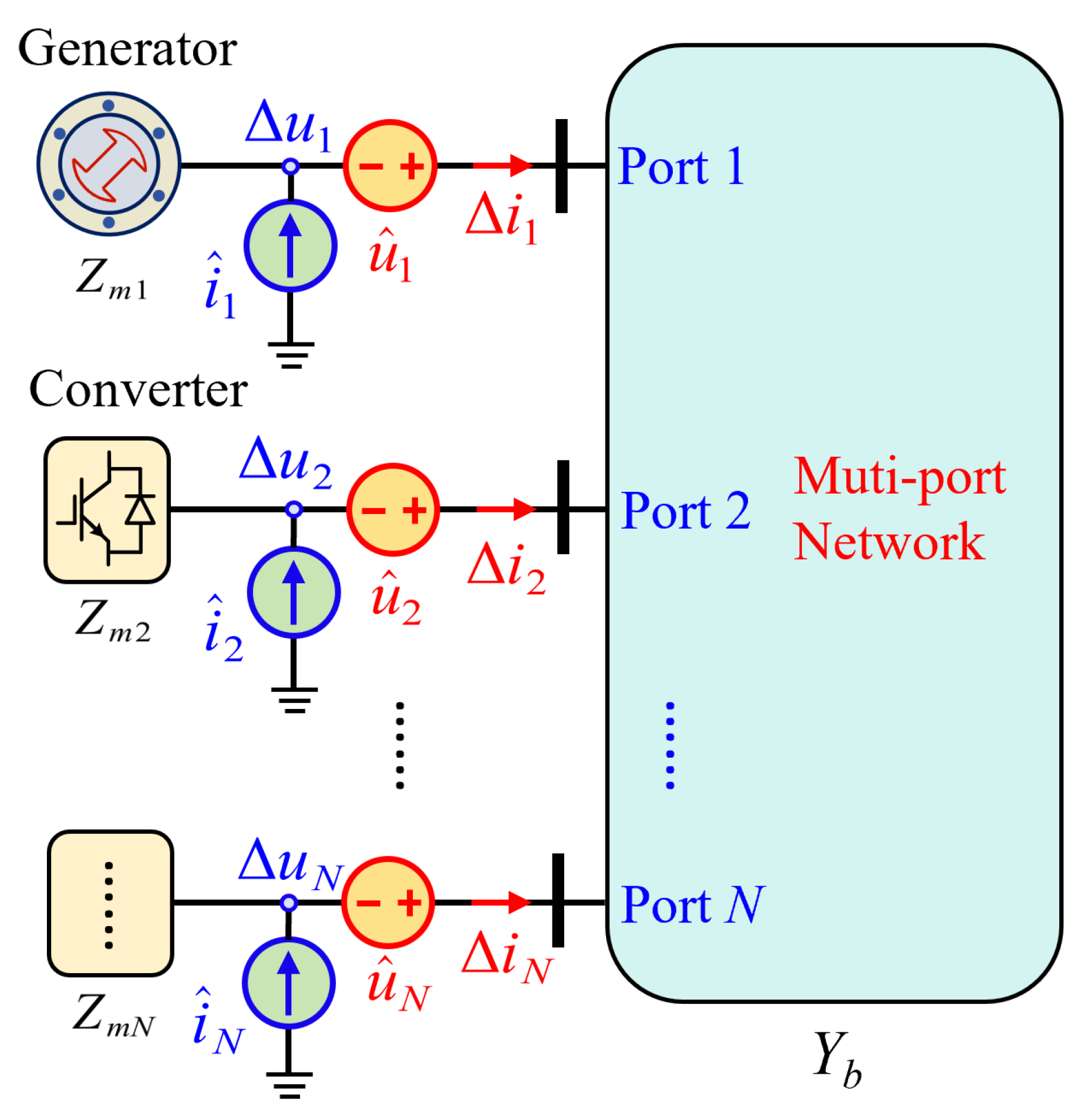
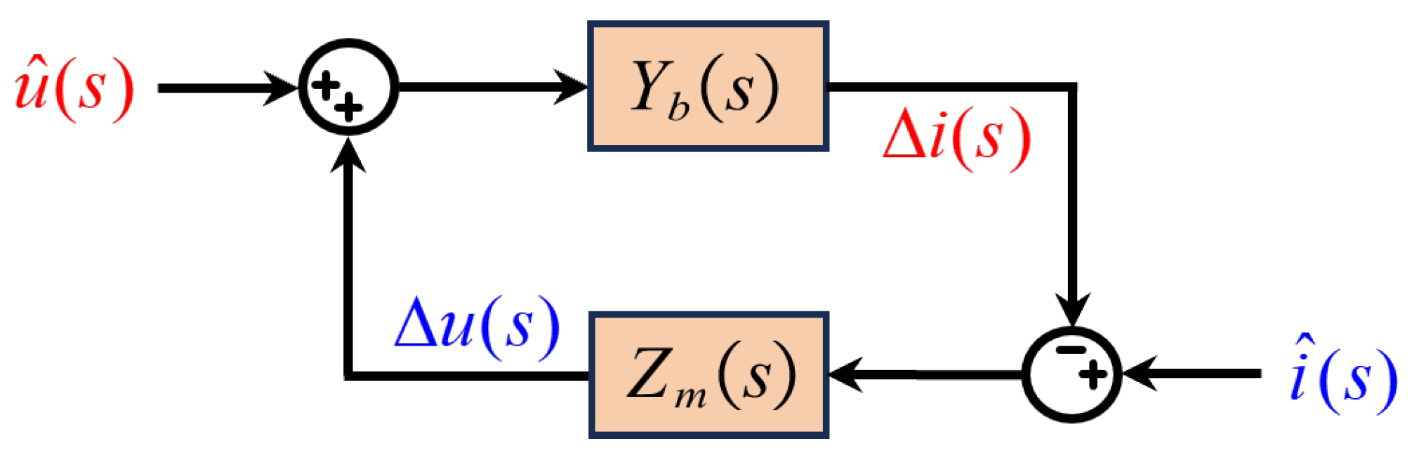
To avoid the conventional source-load separation, two virtual injection variables are introduced at each device port: the virtual voltage injection $\widehat{u}\left(s\right)$ and the virtual current injection $\widehat{i}\left(s\right)$. The schematic of the multi-port voltage and current perturbation injection method for whole-system closed-loop impedance modeling is shown in Figure 5. The actual system responses are defined as the bus-current perturbation $\Delta i\left(s\right)$ and the device-terminal voltage perturbation $\Delta u\left(s\right)$. The physical relationships, also illustrated in Figure 6, are described as follows. The terminal voltage perturbation $\Delta u\left(s\right)$ and the virtual voltage injection $\widehat{u}\left(s\right)$ act on the network admittance matrix $Y_b$ and generate the bus-current perturbation $\Delta i\left(s\right)$. Meanwhile, the bus-current perturbation $\Delta i\left(s\right)$ and the virtual current injection $\widehat{i}\left(s\right)$ act on the device impedance matrix $Z_m$ and generate the terminal voltage perturbation $\Delta u\left(s\right)$. Thus, the closed-loop relationship is established by this structure.

Therefore, the closed-loop interconnection can be written as

$$\left\{\begin{array}{c}\Delta i\left(s\right)=Y_b\left[\widehat{u}\left(s\right)+\Delta u\left(s\right)\right],\hfill \\ \Delta u\left(s\right)=Z_m\left[\widehat{i}\left(s\right)+\Delta i\left(s\right)\right].\hfill \end{array}\right.$$

(26)

When the virtual voltage injection is set to zero, the following relationship can be obtained:

$$\Delta u\left(s\right)=Z_m{\left(I+Y_b{Z}_m\right)}^{-1}·\widehat{i}\left(s\right).$$

(27)

Thus, the closed-loop impedance matrix of the whole system is defined as

$$Z\left(s\right)=Z_m{\left(I+Y_b{Z}_m\right)}^{-1}.$$

(28)

Similarly, when the virtual current injection is set to zero, one has

$$\Delta i\left(s\right)={\left(I+Y_b{Z}_m\right)}^{-1}{Y}_b·\widehat{u}\left(s\right).$$

(29)

Thus, the closed-loop admittance matrix of the whole system is defined as

$$Y\left(s\right)={\left(I+Y_b{Z}_m\right)}^{-1}{Y}_b.$$

(30)

This modeling framework enables the impedance or admittance characteristics at different buses to be extracted from the corresponding elements or submatrices of the whole-system closed-loop matrices. The complete closed-loop system is governed by a common characteristic equation; however, a particular matrix element does not necessarily exhibit every system mode. A mode may be weakly observable at a specific bus, and pole-zero cancellation may further suppress its appearance in the corresponding port transfer function. Therefore, the response extracted at a selected bus should be interpreted as the local observation of the system dynamics from that port. Differences in resonance magnitude among buses indicate different modal visibility and participation at the selected ports rather than guaranteeing that every mode is observable from every matrix element. If bus p is selected as the distribution network interface, its bus admittance characteristic is obtained from the corresponding diagonal submatrix of the whole-system closed-loop admittance matrix.

3.2. Simulation Case Design

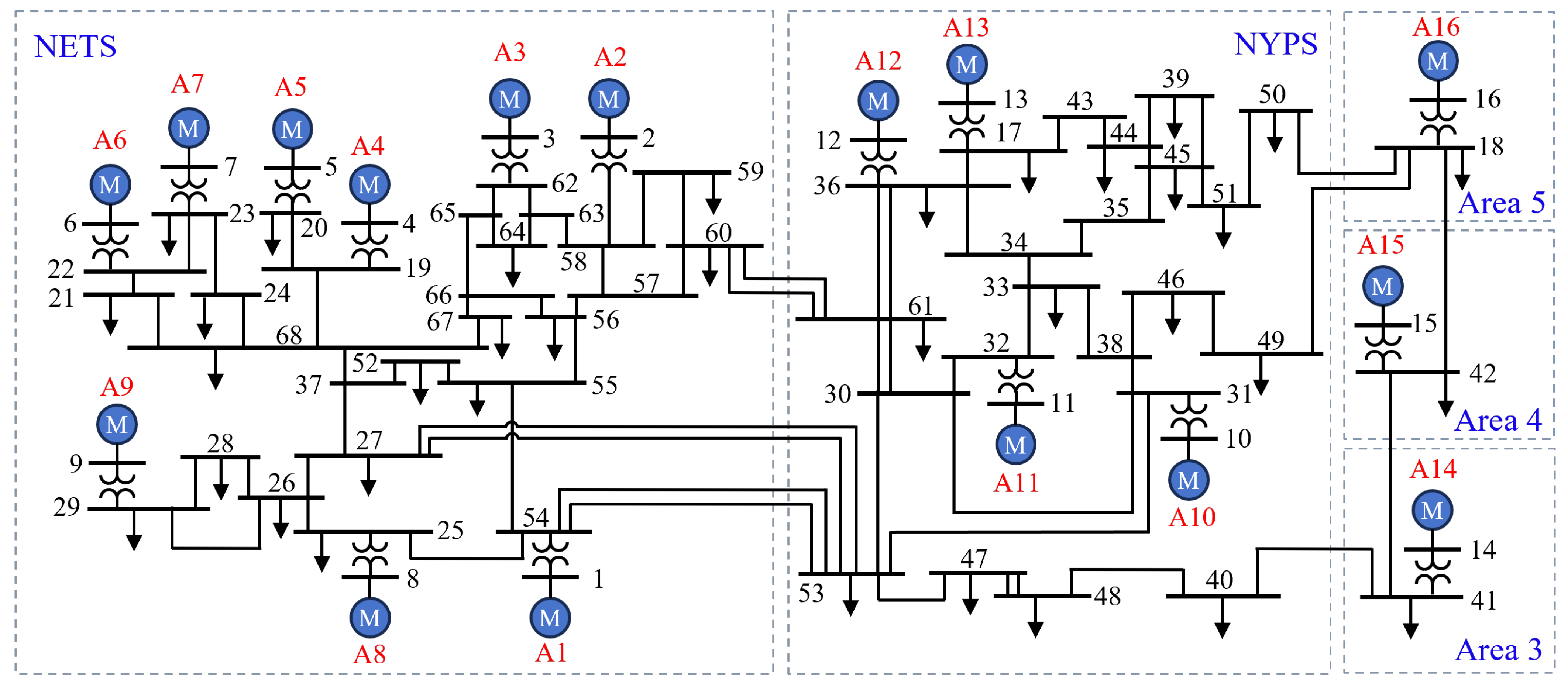
The IEEE 16-machine 68-bus system is a benchmark test system widely used in stability analysis of power systems. It is commonly employed to investigate inter-area low-frequency oscillations, dynamic coupling among generating units, and system damping characteristics in large-scale interconnected AC power grids. The network topology of the system is shown in Figure 7. This system consists of multiple generation areas and a relatively complex interconnection network. It exhibits pronounced SG-dominated dynamics while also capturing cross-area electromagnetic–electromechanical coupling behaviors. Therefore, it is well suited as a test system for studying the evolutionary process from a conventional SG-dominated power grid to a high-penetration power-electronics-dominated grid. Compared with small-scale systems or simplified radial networks, the IEEE 68-bus system can more effectively represent the effects of meshed network topology, multi-source coupling, and inter-area oscillatory modes on the bus characteristics of the main grid.

All modeling and numerical calculations in this study were implemented in MATLAB R2022b. The steady-state operating point of the IEEE 16-machine 68-bus system was obtained through power-flow calculation using the Newton–Raphson method. The dynamic models of the SGs, GFL inverters, and GFM inverters were then linearized around the corresponding steady-state operating points. For each frequency point, the Laplace variable was evaluated as

$$s=j2\pi f,$$

(31)

and the device impedance matrix $Z_m\left(s\right)$ and network admittance matrix $Y_b\left(s\right)$ were calculated numerically. The whole-system closed-loop impedance/admittance matrices were subsequently obtained according to the formulation described in Section 3.1. The frequency responses were evaluated over the range of 0.1–3000 Hz using 500 logarithmically spaced frequency points. All matrix calculations were performed using MATLAB double precision arithmetic, and the positive-sequence bus admittance was extracted from the resulting whole-system matrix for Bode plot presentation and quantitative comparison.

The central issue addressed in this section is whether the port characteristics of the main grid observed at the PCC of the distribution network remain similar to those of a conventional strong grid as SGs are progressively replaced by GFL and GFM devices, or whether new dynamic behaviors emerge with increasing penetration of power-electronic devices. In conventional analyses, the main grid generally exhibits relatively “stiff” port characteristics, namely, strong voltage-support capability and stable phase characteristics over a wide frequency range. However, as the proportion of SGs decreases, system inertia declines, and the synchronization mechanism gradually shifts from mechanical rotor coupling to PLL-based synchronization or grid-forming control, the bus characteristics of the main grid are no longer determined solely by network parameters, but are jointly influenced by device control strategies, inertia levels, synchronization mechanisms, and their spatial distributions. Under such conditions, the equivalent bus admittance of the main grid viewed from distribution networks reflects not only the network topology and electrical distance, but also, to a significant extent, the dynamic interactions among power-electronic devices.

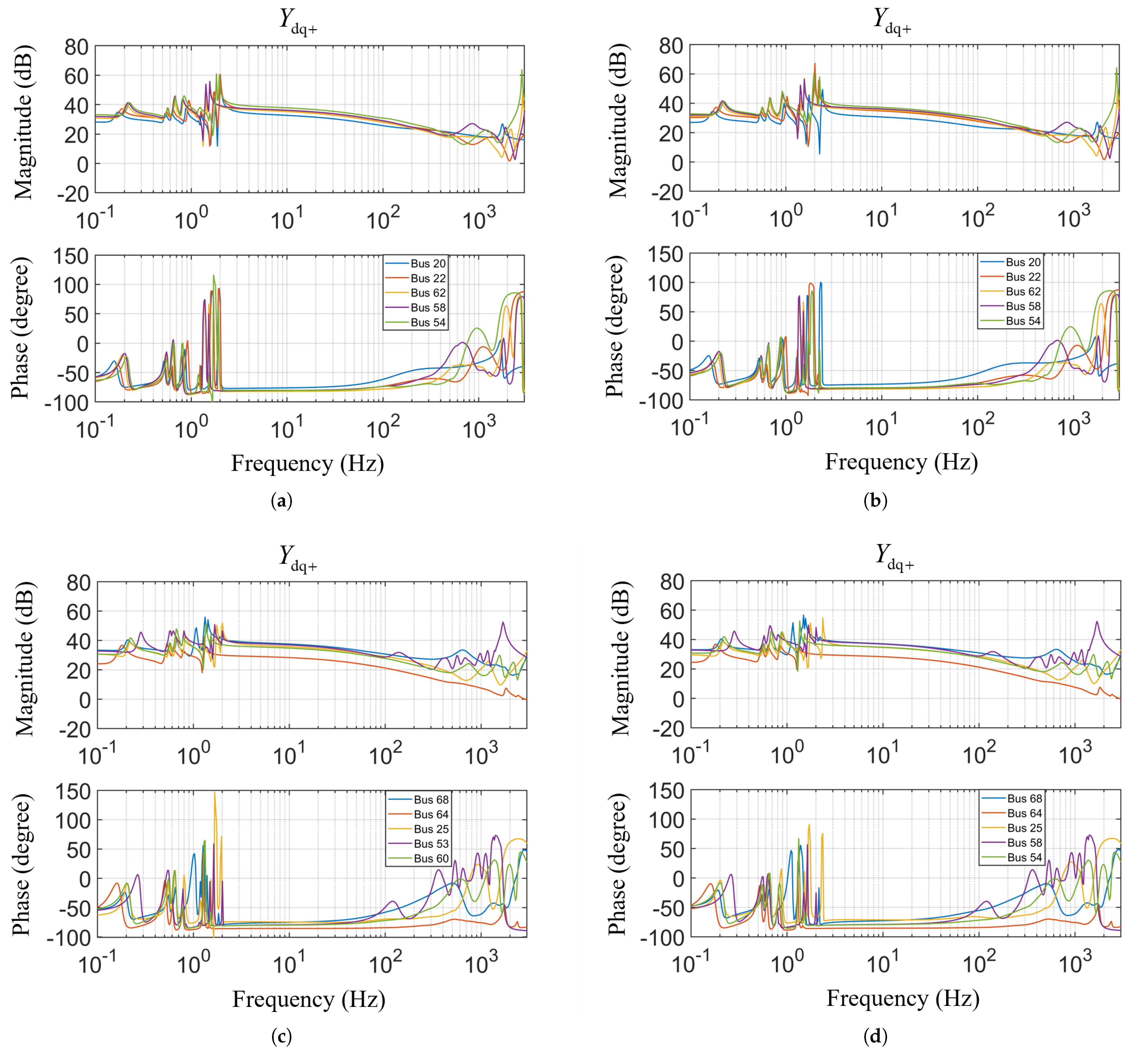
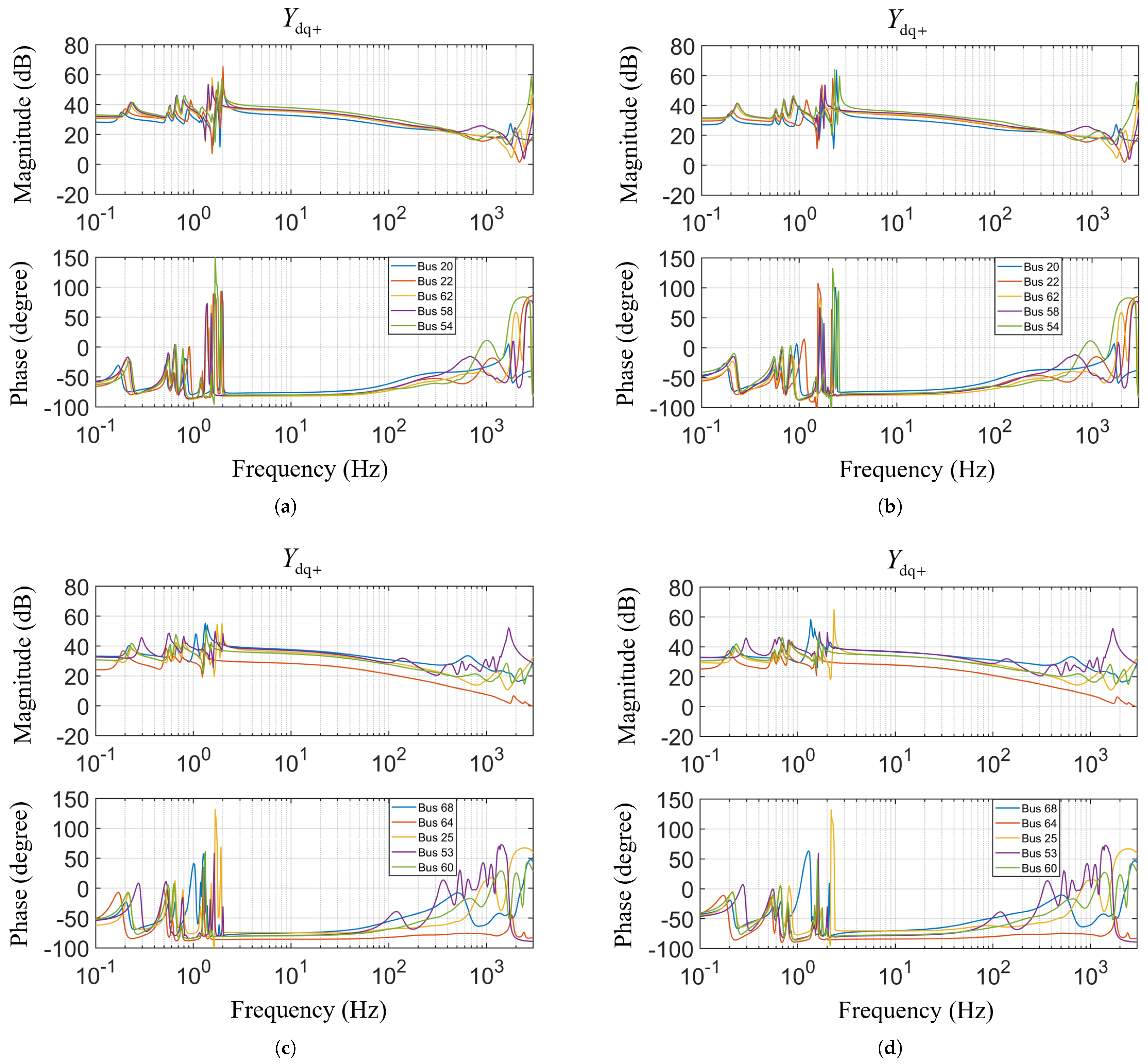
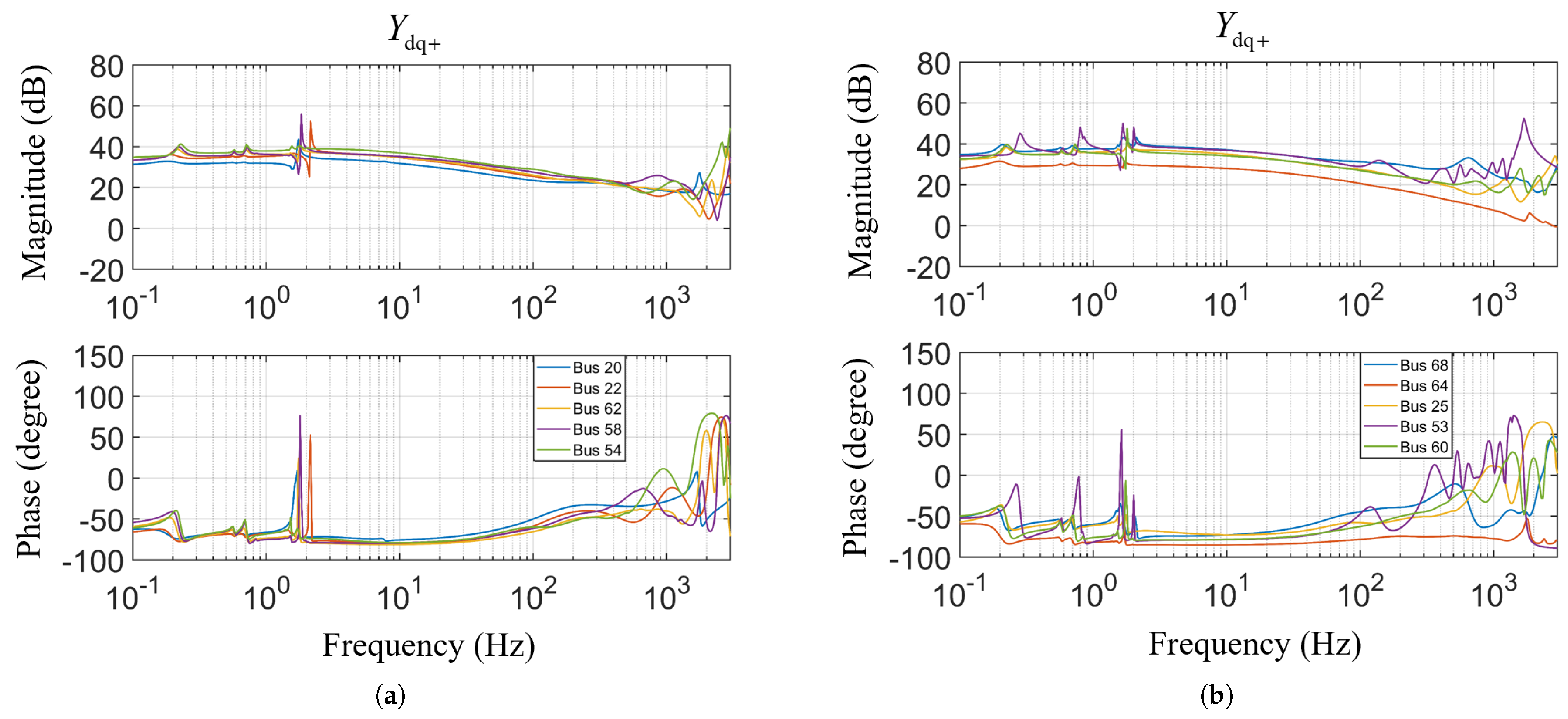
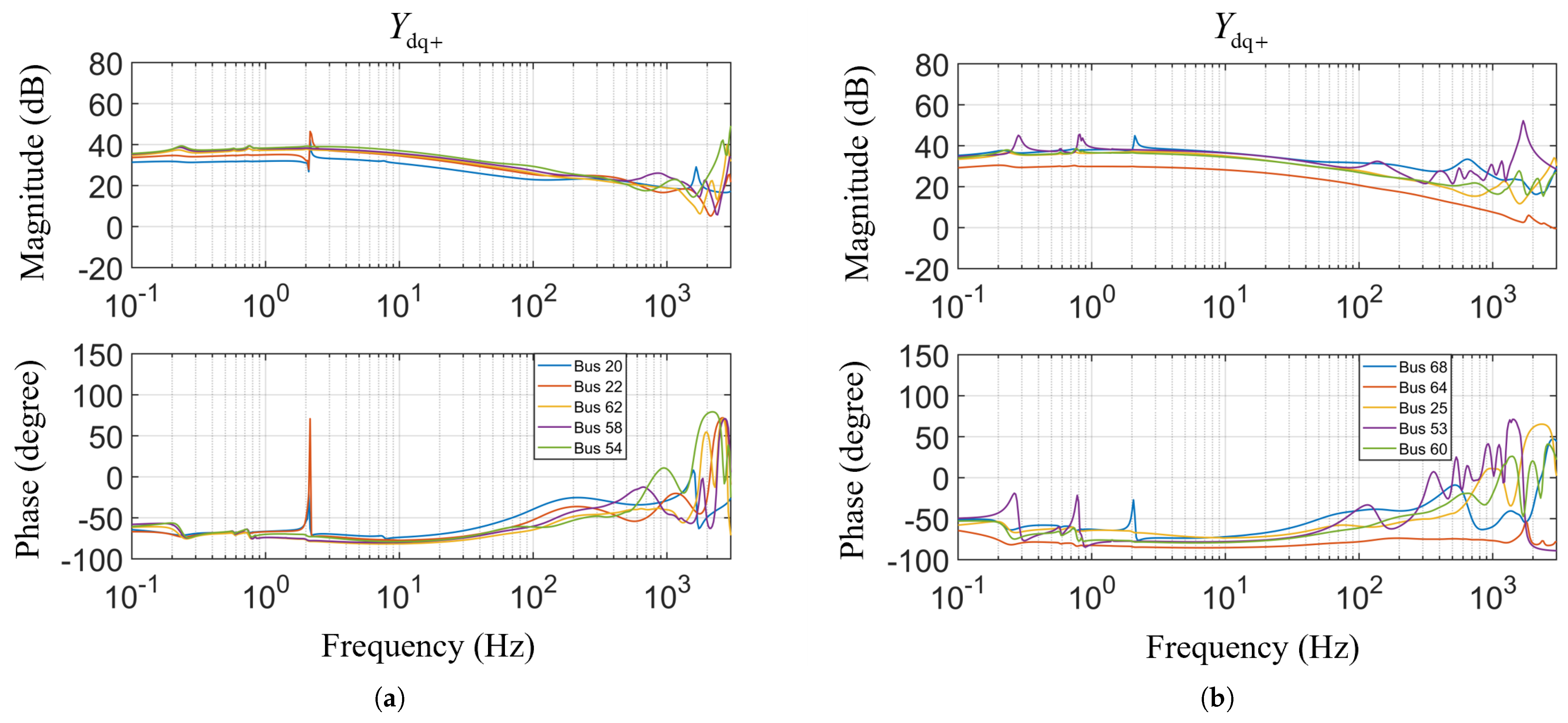
Specifically, several candidate distribution-network access nodes are first selected in the system, including nodes electrically close to power generation sources and nodes with intermediate electrical distances from SGs, so as to compare the influence of different access locations on the bus characteristics. Under the condition that the overall active-power balance of the system is maintained, the power shares of GFL and GFM devices are gradually increased. For each scenario, the equivalent bus admittance matrix of the main grid at the candidate access points is extracted. After coordinate transformation, the frequency-domain response of the positive-sequence admittance, denoted as $Y_{\mathrm{dq}+}$, is obtained. Finally, Bode plots are used to compare the magnitude and phase characteristics of the main-grid port under different operating conditions. The obtained bus admittance is used not only to characterize the dynamic “stiffness” of the main grid at the distribution-network access point, but also to reflect the frequency response capability of the main grid to external disturbances and its potential resonance sensitivity under different penetration levels of power-electronic devices. The detailed configurations of the five simulation scenarios are listed in

Table 4. Configuration of the 100% SG benchmark scenario.

Base Power ${\mathit{S}}_{\mathbf{base}}$		100 MVA
Base Frequency ${\mathit{f}}_{\mathbf{base}}$		60 Hz
Source Type	Bus	Inertia $\mathit{H}$ (s)	Damping (pu)	Active Power (pu)
SG (100%)	1	42.0	10.50	2.50
	2	30.2	7.55	5.45
	3	35.8	8.95	6.50
	4	28.6	7.15	6.32
	5	26.0	6.50	5.05
	6	34.8	8.70	7.00
	7	26.4	6.60	5.60
	8	24.3	6.075	5.40
	9	34.5	8.625	8.00
	10	31.0	7.75	5.00
	11	28.2	7.05	10.00
	12	92.3	23.075	13.50

,

Table 5. Configuration of the 20% GFL penetration scenario.

Base Power ${\mathit{S}}_{\mathbf{base}}$		100 MVA
Base Frequency ${\mathit{f}}_{\mathbf{base}}$		60 Hz
Source Type	Bus	Inertia $\mathit{H}$ (s)	Damping (pu)	Active Power (pu)
SG (80%)	1	42.0	10.50	2.50
	2	30.2	7.55	5.45
	3	35.8	8.95	6.50
	4	28.6	7.15	6.32
	5	26.0/9.5	6.50/2.40	1.85
	6	34.8	8.70	7.00
	7	26.4/11.3	6.60/2.80	2.40
	8	24.3/9.9	6.075/2.50	2.20
	9	34.5/6.9	8.625/1.70	1.60
	10	31.0	7.75	5.00
	11	28.2	7.05	10.00
	12	92.3	23.075	13.50
GFL (20%)	20	–	–	3.20
	23	–	–	3.20
	26	–	–	3.20
	28	–	–	3.20
	29	–	–	3.20

For entries expressed as $A/B$ (such as 26.0/9.5), A corresponds to the case where the SG remains online with reduced active power, whereas B corresponds to the case where the associated SG is decommissioned.

,

Table 6. Configuration of the 40% GFL penetration scenario.

Base Power ${\mathit{S}}_{\mathbf{base}}$		100 MVA
Base Frequency ${\mathit{f}}_{\mathbf{base}}$		60 Hz
Source Type	Bus	Inertia $\mathit{H}$ (s)	Damping (pu)	Active Power (pu)
SG (60%)	1	42.0/15.1	10.50/3.80	0.90
	2	30.2/12.5	7.55/3.10	2.25
	3	35.8/18.2	8.95/4.60	3.30
	4	28.6	7.15	6.32
	5	26.0/9.5	6.50/2.40	1.85
	6	34.8/18.9	8.70/4.70	3.80
	7	26.4/11.3	6.60/2.80	2.40
	8	24.3/9.9	6.075/2.50	2.20
	9	34.5/6.9	8.625/1.70	1.60
	10	31.0	7.75	5.00
	11	28.2	7.05	10.00
	12	92.3/59.5	23.075/14.90	8.70
GFL (40%)	20	–	–	3.20
	22	–	–	3.20
	23	–	–	3.20
	26	–	–	3.20
	28	–	–	3.20
	29	–	–	3.20
	36	–	–	4.80
	54	–	–	1.60
	58	–	–	3.20
	62	–	–	3.20

For entries expressed as $A/B$ (such as 26.0/9.5), A corresponds to the case where the SG remains online with reduced active power, whereas B corresponds to the case where the associated SG is decommissioned.

,

Table 7. Configuration of the 45% SG, 15% GFM, and 40% GFL scenario.

Base Power ${\mathit{S}}_{\mathbf{base}}$		100 MVA
Base Frequency ${\mathit{f}}_{\mathbf{base}}$		60 Hz
Source Type	Bus	Inertia $\mathit{H}$ (s)	Damping (pu)	Active Power (pu)
SG (45%)	2	12.5	3.10	2.25
	4	28.6	7.15	6.32
	7	11.3	2.80	2.40
	9	6.9	1.70	1.60
	10	31.0	7.75	5.00
	11	28.2	7.05	10.00
	12	59.5	14.90	8.70
GFL (40%)	20	–	–	3.20
	22	–	–	3.20
	23	–	–	3.20
	26	–	–	3.20
	28	–	–	3.20
	29	–	–	3.20
	36	–	–	4.80
	54	–	–	1.60
	58	–	–	3.20
	62	–	–	3.20
GFM (15%)	1	15.1	1510	0.90
	3	18.2	1820	3.30
	5	9.5	950	1.85
	6	18.9	1890	3.80
	8	9.9	990	2.20

and

Table 8. Configuration of the 15% SG, 25% GFM, and 60% GFL scenario.

Base Power ${\mathit{S}}_{\mathbf{base}}$		100 MVA
Base Frequency ${\mathit{f}}_{\mathbf{base}}$		60 Hz
Source Type	Bus	Inertia $\mathit{H}$ (s)	Damping (pu)	Active Power (pu)
SG (15%)	4	28.6	7.15	1.82
	7	11.3	2.80	2.40
	12	59.5	14.90	8.00
GFL (60%)	11	–	–	10.00
	20	–	–	4.70
	22	–	–	5.50
	23	–	–	4.70
	26	–	–	3.20
	28	–	–	3.20
	29	–	–	3.20
	36	–	–	5.50
	54	–	–	1.60
	58	–	–	3.20
	62	–	–	3.50
GFM (25%)	1	15.1	1510	0.90
	2	12.5	1250	2.25
	3	18.2	1820	3.00
	5	9.5	950	1.85
	6	14.9	1490	3.00
	8	9.9	990	2.20
	9	6.9	690	1.60
	10	31.0	3100	5.00

.

The five scenarios are designed to form a progressive and interpretable transition in source composition rather than to predict a unique future generation mix. Scenario 1, consisting entirely of SGs, is used as the conventional reference case. In Scenarios 2 and 3, the GFL share is increased to 20% and 40%, respectively, using an interval of 20 percentage points to represent the transition from an initial level of GFL integration to a relatively high penetration level. For both scenarios, the cases with the corresponding SGs retained online and disconnected are considered separately, so that the influence of increasing GFL power share can be distinguished from the additional effect caused by the actual loss of synchronous inertia and support.

Scenario 4 retains the GFL share at 40% while introducing 15% GFM capacity and reducing the SG share accordingly. This configuration represents an intermediate stage in which GFM technology begins to provide supplementary grid support, and, more importantly, allows the effect of GFM integration to be examined by comparison with Scenario 3 without simultaneously changing the GFL share. Scenario 5 further increases the GFL share to 60%, while 25% GFM and 15% SG are retained. Previous studies have shown that the GFM capacity required for adequate small-signal stability is system dependent and varies with grid strength, network topology, and the desired stability margin [18]. Recent multi-bus studies have also reported that GFM shares on the order of 30–40% can provide stable operation in fully inverter-based benchmark systems [23]. Therefore, the 25% GFM share adopted here is not intended as a universal stability threshold, but as a representative relatively high GFM penetration level. Meanwhile, retaining a limited proportion of SGs reflects a possible future hybrid grid in which synchronous generation is substantially reduced but not completely eliminated. These scenarios therefore provide a continuous comparison from an SG-dominated system to GFL-rich operation and finally to a system with high power-electronic penetration supported jointly by SGs and GFM inverters.

In the IEEE 16-machine 68-bus system, areas 3, 4, and 5 are represented by equivalent SGs corresponding to external power grids. Therefore, directly replacing any of these equivalent SGs with a GFL or GFM inverter to represent an entire external regional grid is not physically appropriate from a practical system perspective. For this reason, the simulation cases are designed only within the NETS and NYPS areas, where individual SGs can be more reasonably replaced by power-electronic devices.

For the system-level cases, the control bandwidths are kept unchanged for inverters of the same type, while the physical filter and controller parameters are scaled according to the rated capacity of each inverter. The PI gains are then recalculated from the scaled $L_f$ and $C_f$ according to the bandwidth-based design relations given in Table 2 and Table 3. The original bus, transmission line, transformer, load, and SG parameters of the IEEE 16-machine 68-bus benchmark system are provided in [24]. These standard parameters are therefore not repeated here.

4. Simulation Results and Analysis

4.1. Results Under Different Source Compositions

4.1.1. 100% SG Scenario

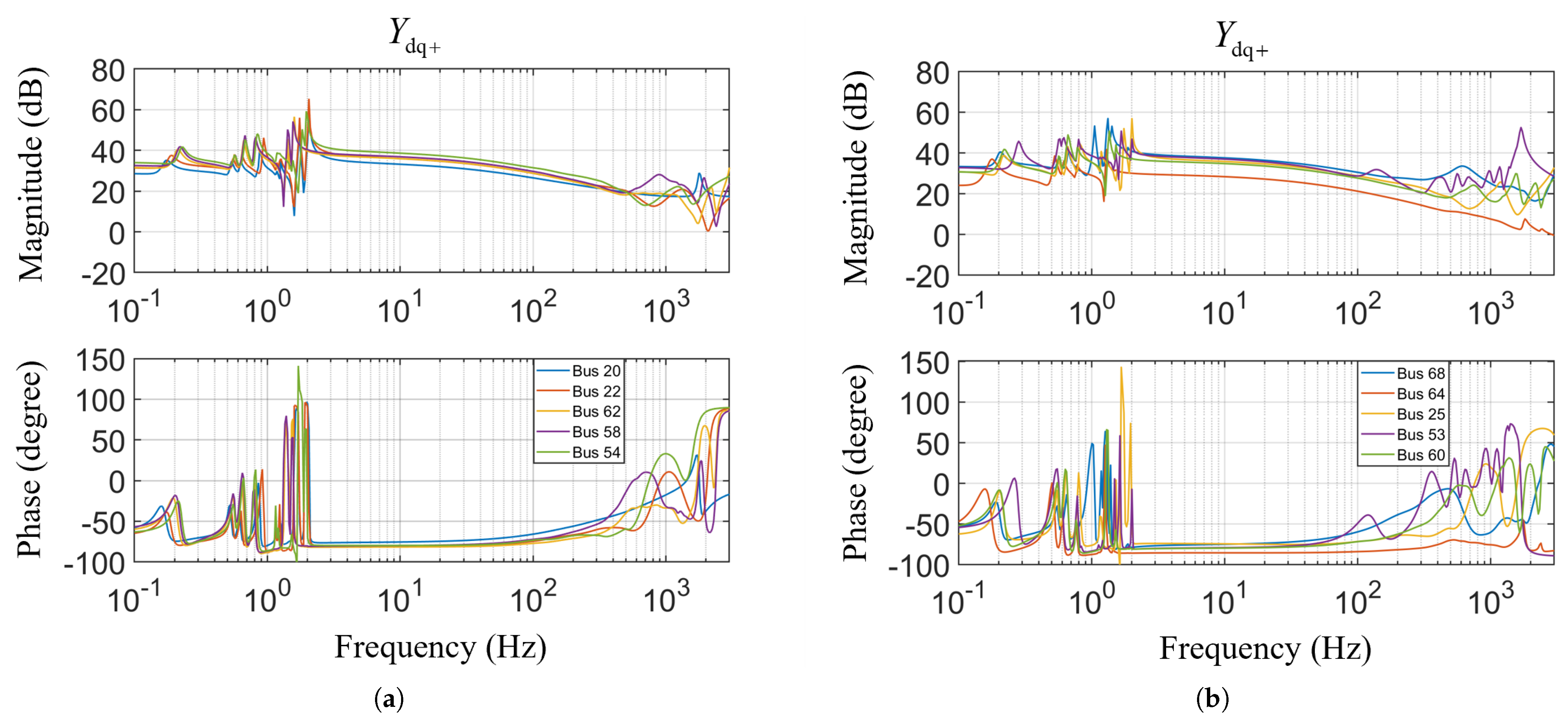
First, a benchmark operating condition is established, in which all 16 machines in the system are modeled as SGs, forming a conventional SG-dominated main grid. This scenario is used to characterize the baseline bus characteristics of a conventional high-inertia AC grid. In this paper, several access nodes are selected under this operating condition, including nodes located close to SGs and nodes with intermediate electrical distances from SGs, so as to compare the equivalent bus admittance characteristics observed at different access locations. This scenario is used to investigate whether the conventional SG-dominated main grid exhibits clearly different port “stiffness” at different access locations. The benchmark scenario also provides a reference for subsequent cases involving power-electronic devices. The simulation results are shown in Figure 8.

4.1.2. 20% GFL Penetration Scenario

On the basis of the benchmark scenario, GFL inverters with a power share of 20% are introduced. Considering that GFL devices may suffer from synchronization stability issues under weak-grid conditions, they are preferentially connected to several nodes located close to SGs, so as to enhance their grid-connection stability and avoid masking their intrinsic influence on the main-grid port characteristics due to excessively weak access locations. In this scenario, two subcases are further considered. In the first subcase, the SGs only reduce their active-power output to offset the additional power supplied by the GFL inverters, while remaining in service; that is, the redundant SGs are retained as spinning reserves. In the second subcase, the corresponding replaced SGs are directly disconnected from the grid, and the GFL inverters practically take over their power-support role. The comparison between these two subcases essentially distinguishes two different evolutionary paths: increased power-electronic generation with SG inertia retained and actual replacement of SGs by power-electronic devices accompanied by inertia reduction. The former mainly reflects the impact of changes in control strategies, whereas the latter additionally involves changes in inertia, damping, and short-circuit support capability caused by the decommissioning of SGs. The simulation results are shown in Figure 9.

4.1.3. 40% GFL Penetration Scenario

The power share of GFL inverters is further increased to 40%, while the same two subcases are considered, namely, “SG output reduction with generators retained online” and “direct disconnection of SGs”. Compared with the 20% GFL scenario, power-electronic devices account for a higher proportion of the system in this case, and their influence on the main-grid bus characteristics is expected to become more pronounced. In particular, when SGs are actually decommissioned, factors such as the reduction in equivalent system inertia and the enhancement of PLL-dominated synchronization dynamics may be reflected in the bus admittance spectra. Meanwhile, as conventional synchronous support weakens, the sensitivity of the system to operating-point variations and disturbances may further increase, leading to more evident differences in the port characteristics observed at different access points. This scenario is used to examine whether, at a relatively high GFL penetration level, the main-grid port characteristics can still retain the characteristics of a conventional SG-dominated grid, or whether they have begun to exhibit a clear power-electronics-dominated tendency. The simulation results are shown in Figure 10.

4.1.4. 45% SG + 15% GFM + 40% GFL Scenario

On the basis of Scenario 3, GFM inverters are further introduced, that is, part of the SGs are replaced by GFM inverters, forming a hybrid generation structure consisting of 45% SG, 15% GFM, and 40% GFL. The purpose of this scenario is to analyze whether an appropriate introduction of GFM inverters can improve the main-grid port characteristics when the system already has a relatively high GFL penetration level. Compared with GFL inverters, GFM inverters generally provide stronger voltage-establishment capability and frequency-support capability. Therefore, from the perspective of port characteristics, the introduction of GFM devices is expected to enhance the equivalent “stiffness” of the main grid over certain frequency ranges and mitigate the port-admittance magnitude attenuation or phase anomalies caused by the increased GFL share. By comparing this scenario with Scenario 3, the role of GFM inverters in reshaping the external characteristics of the main grid can be further identified, namely, whether they can partially restore the bus characteristics of a conventional SG-dominated system, or instead form a new set of dynamic characteristics between an SG-dominated main grid and a high-GFL-penetration main grid. The simulation results are shown in Figure 11.

4.1.5. 15% SG + 25% GFM + 60% GFL Scenario

Finally, a high power-electronic penetration scenario with 15% SG, 25% GFM, and 60% GFL is configured. This scenario can be regarded as a possible future operating condition of the main grid. Although the proportion of SGs is substantially reduced, they are not completely eliminated. Meanwhile, driven by sustainable development requirements, GFL devices still account for a relatively high proportion, enabling the integration of renewable energy sources such as wind and photovoltaic generation. In contrast, GFM devices serve as a key supplement to enhance the system’s voltage and frequency support capability, improve system dynamic characteristics, and continue to fulfill the role originally played by SGs. The significance of this scenario lies in examining, from a more forward-looking perspective, the possible form of the main-grid bus characteristics in future power systems, specifically, under a hybrid structure comprising a small number of SGs, a relatively high proportion of GFM inverters, and a higher proportion of GFL inverters. This scenario analyzes whether the main grid observed from the distribution-network access point can still be approximately regarded as a conventional strong grid, or whether its bus admittance exhibits new dynamic characteristics. Furthermore, this scenario helps reveal the role of GFM inverters in reshaping the external characteristics of the main grid in high power-electronic systems, as well as the extent to which they can mitigate the port-weakening tendency in conventional GFL-dominated scenarios. The study of this scenario provides a reference for future transmission–distribution interface modeling and the grid-connection control design of power-electronic devices in distribution networks. The simulation results are shown in Figure 12.

4.2. Quantitative Analysis

The five scenarios considered in this study describe the progressive change of the main grid from an SG-dominated generation structure to a system with a high proportion of GFL and GFM inverters. In addition to the qualitative comparison of the Bode plots, several quantitative indicators are introduced to characterize the changes in the bus admittance spectra. Let

$$M_k\left(f\right)=20{\log }_{10}\left|Y_k\left(j2\pi f\right)\right|$$

(32)

denote the magnitude of the positive-sequence bus admittance at the kth observation bus.

The selected observation buses are divided into two groups: buses close to generator buses, denoted by ${\mathcal{B}}_{\mathrm{c}}$, and buses electrically remote from generator buses, denoted by ${\mathcal{B}}_{\mathrm{r}}$. For each bus group $g\in \{\mathrm{c},\mathrm{r}\}$, the dominant low-frequency peak is defined as

$$P_{\mathrm{LF}}^{\left(g\right)}=\underset{\begin{array}{c}k\in {\mathcal{B}}_g\\ f\in [0.2,3]\mathrm{Hz}\end{array}}{\max }{M}_k\left(f\right),$$

(33)

where $P_{\mathrm{LF}}^{\left(g\right)}$ represents the largest bus admittance magnitude observed within the selected low-frequency range for bus group g. The corresponding frequency is denoted by $f_{\mathrm{LF}}^{\left(g\right)}$. These two quantities are used to describe the magnitude and location of the dominant low-frequency peak, respectively.

Second, to quantify the smoothness of the low-frequency admittance spectrum, the average low-frequency magnitude variation is defined as

$$R_{\mathrm{LF}}={\displaystyle \frac{1}{N}}{\displaystyle \sum _{k=1}^N}\left[\underset{f\in [0.2,3]\mathrm{Hz}}{\max }{M}_k\left(f\right)-\underset{f\in [0.2,3]\mathrm{Hz}}{\min }{M}_k\left(f\right)\right].$$

(34)

A smaller $R_{\mathrm{LF}}$ indicates a smoother low-frequency admittance spectrum with fewer abrupt magnitude variations. It should be emphasized that $R_{\mathrm{LF}}$ is used only as a descriptive quantity for comparing the frequency responses and is not a stability margin.

Finally, the spatial dispersion among different observation buses is evaluated by

$$D\left(f\right)=\underset{k}{\max }{M}_k\left(f\right)-\underset{k}{\min }{M}_k\left(f\right).$$

(35)

In the following discussion, $D\left(100\mathrm{Hz}\right)$ is used to compare the spatial dispersion among buses while avoiding the dominant low-frequency resonance region.

First, the benchmark case with 100% SGs represents the conventional SG-dominated main grid. As shown in

Table 9. Dominant low-frequency bus admittance peaks under different generation scenarios.

Scenario	Close to Generator Buses		Remote from Generator Buses
	${\mathit{P}}_{\mathbf{LF}}$ (dB)	${\mathit{f}}_{\mathbf{LF}}$ (Hz)	${\mathit{P}}_{\mathbf{LF}}$ (dB)	${\mathit{f}}_{\mathbf{LF}}$ (Hz)
100% SG	66.2	2.03	57.3	1.32
20% GFL, SG retained	61.9	2.04	56.1	1.30
20% GFL, SG disconnected	67.6	1.98	58.0	1.50
40% GFL, SG retained	66.3	1.95	56.2	1.32
40% GFL, SG disconnected	65.1	2.46	66.0	2.44
45% SG + 15% GFM + 40% GFL	56.2	1.87	52.0	1.68
15% SG + 25% GFM + 60% GFL	47.8	2.20	45.8	0.86

, the dominant low-frequency peak is approximately 66.2 dB at 2.03 Hz for the buses close to generator buses and 57.3 dB at 1.32 Hz for the electrically remote buses. The difference between the two bus groups is not limited to the dominant resonance. At 100 Hz, the magnitude dispersion among the close buses is approximately 4.9 dB, whereas that among the remote buses reaches approximately 9.4 dB. Therefore, even in the conventional SG-dominated system, the equivalent bus admittance is not spatially uniform. The larger dispersion observed at remote buses indicates that electrical distance and network topology already influence the dynamic boundary seen from different distribution network access points.

Second, the 20% GFL scenario illustrates the difference between increasing power-electronic generation while retaining synchronous machines and actually removing synchronous machines from service. When the SGs remain online with reduced active power, the dominant peaks are approximately 61.9 dB and 56.1 dB for the close and remote bus groups, respectively. When the corresponding SGs are disconnected, these values increase to approximately 67.6 dB and 58.0 dB. Thus, under the same 20% GFL penetration, SG disconnection increases the dominant peak by approximately 5.7 dB at the close buses and 1.9 dB at the remote buses. This comparison indicates that the change in bus admittance cannot be explained only by the active power share of GFL inverters. Whether the replaced SGs remain synchronously connected to the system also affects the observed frequency response because their electromechanical dynamics and synchronous support are retained in the former case but removed in the latter.

When the GFL share is further increased to 40%, the effect becomes more strongly dependent on the observation location. With SGs retained online, the dominant peaks are approximately 66.3 dB at 1.95 Hz for the close buses and 56.2 dB at 1.32 Hz for the remote buses. After the corresponding SGs are disconnected, the close bus peak changes only slightly to 65.1 dB, whereas the remote bus peak increases substantially to 66.0 dB. The dominant remote bus peak therefore increases by approximately 9.8 dB, and its frequency shifts from approximately 1.32 Hz to 2.44 Hz. The close bus dominant frequency also shifts from approximately 1.95 Hz to 2.46 Hz. These results show that SG decommissioning does not simply cause a uniform increase in the bus admittance peaks. Instead, it redistributes the low-frequency resonance characteristics among different locations and changes both their magnitude and dominant frequency. This location-dependent redistribution becomes particularly evident when the GFL share is high and synchronous support is substantially reduced.

The comparison between the 20% and 40% GFL cases further supports this observation. For the SG retained cases, increasing the GFL proportion from 20% to 40% raises the close bus dominant peak from 61.9 dB to 66.3 dB, while the remote bus peak remains almost unchanged at approximately 56 dB. In contrast, for the SG disconnected cases, the close bus peak decreases slightly from 67.6 dB to 65.1 dB, whereas the remote bus peak increases from 58.0 dB to 66.0 dB. Therefore, increasing GFL penetration should not be interpreted as producing a monotonic increase in resonance magnitude at all buses. A more appropriate interpretation is that the combination of GFL penetration and SG decommissioning changes the spatial distribution and frequency characteristics of the system modes, and these changes are reflected differently at different bus locations.

Third, the introduction of GFM inverters has a pronounced effect on the low-frequency bus admittance characteristics. Taking the 40% GFL case with the corresponding SGs disconnected as the reference before GFM integration, introducing 15% GFM capacity reduces the dominant low-frequency peak from approximately 65.1 dB to 56.2 dB for the close bus group, corresponding to a reduction of 8.9 dB. For the remote bus group, the peak decreases from approximately 66.0 dB to 52.0 dB, corresponding to a larger reduction of approximately 14.0 dB.

The smoothing effect is even more evident from $R_{\mathrm{LF}}$. It can be found in

Table 10. Quantitative comparison of low-frequency magnitude variation and spatial dispersion.

Scenario	${\mathit{R}}_{\mathbf{LF}}$ (dB)		D(100 Hz) (dB)
	Close	Remote	Close	Remote
100% SG	34.9	23.6	4.9	9.4
20% GFL, SG retained	33.1	22.4	5.5	9.4
20% GFL, SG disconnected	31.0	21.5	6.7	9.8
40% GFL, SG retained	31.8	22.7	5.1	9.7
40% GFL, SG disconnected	32.9	23.3	5.6	10.3
45% SG + 15% GFM + 40% GFL	12.3	8.6	5.7	10.5
15% SG + 25% GFM + 60% GFL	5.0	4.5	6.4	11.0

that, before GFM integration, $R_{\mathrm{LF}}$ is approximately 32.9 dB for the close buses and 23.3 dB for the remote buses. After 15% GFM is introduced, these values decrease to approximately 12.3 dB and 8.6 dB, corresponding to reductions of 20.6 dB and 14.7 dB, respectively. Therefore, the effect of GFM integration is not limited to reducing an individual resonance peak. It substantially reduces the overall magnitude variation over the low-frequency range and makes the bus admittance spectra considerably smoother. This quantitatively supports the observation from the Bode plots that GFM inverters reshape the low-frequency dynamic characteristics of the main grid.

Finally, Scenario 5 represents a system with only 15% SG capacity, 25% GFM capacity, and 60% GFL capacity. Although the GFL share is further increased, the dominant peaks decrease to approximately 47.8 dB for the close buses and 45.8 dB for the remote buses. Compared with Scenario 4, these values are further reduced by approximately 8.4 dB and 6.2 dB, respectively. The corresponding $R_{\mathrm{LF}}$ values decrease from 12.3 dB to 5.0 dB for the close buses and from 8.6 dB to 4.5 dB for the remote buses. Hence, the high power-electronic penetration scenario does not reproduce the low-frequency spectrum of the original SG-dominated system. Instead, it exhibits a substantially smoother low-frequency admittance characteristic shaped by the control dynamics of the GFM and GFL inverters.

Nevertheless, GFM integration does not eliminate the dependence of the bus admittance on network location. Across all investigated scenarios, $D\left(100\mathrm{Hz}\right)$ remains within approximately 4.9–6.7 dB for the buses close to generation sources, whereas the corresponding dispersion for the remote buses is approximately 9.4–11.0 dB. In Scenario 5, for example, the dispersion is approximately 6.4 dB for the close bus group and 11.0 dB for the remote bus group. Therefore, although GFM integration significantly smooths the low-frequency response, the differences caused by electrical distance and network topology remain clearly observable.

Overall, the quantitative results reveal three main characteristics of the evolution of the upstream grid bus admittance. First, SG decommissioning and increasing GFL penetration reshape rather than uniformly amplify the low-frequency resonance characteristics, and the resulting changes depend strongly on the observation location. Second, introducing GFM inverters significantly reduces both the dominant low-frequency peaks and the overall low-frequency magnitude variation, demonstrating their ability to reshape the dynamic bus characteristics of a system with high GFL penetration. Third, the spatial dispersion among different buses remains significant even at high GFM penetration. Consequently, the future upstream grid should not be represented by a single fixed equivalent that is independent of generation composition, observation location, and frequency range. From the perspective of transmission and distribution interface modeling, a dynamic bus admittance representation that reflects these factors is therefore more appropriate.

Although GFM inverters help the main grid exhibit characteristics closer to those of an ideal voltage source in modeling, their underlying shaping mechanism differs from that of conventional SGs. A conventional SG-dominated power system is typically a high-inertia, low-damping system. The large inertia of SGs is mainly determined by the mechanical structure of the rotor and is therefore difficult to change significantly over a short time scale. Although the damping level can be improved through supplementary control, it is still fundamentally constrained by the physical system and operating conditions.

In contrast, for GFM inverters adopting the classical droop control strategy with a low-pass filter, the equivalent inertia J and damping D are given by:

$$\left\{\begin{array}{cc}\hfill J\hfill & ={\displaystyle \frac{1}{m_p·f_{droop}·2\pi }},\hfill \\ \hfill D\hfill & ={\displaystyle \frac{1}{m_p}}.\hfill \end{array}\right.$$

(36)

It can be readily observed that, for the droop-controlled GFM considered here, the equivalent inertia and damping are related through

$${\displaystyle \frac{D}{J}}=2\pi f_{droop}={\omega }_{droop}.$$

(37)

Therefore, J and D should not be directly compared by their numerical magnitudes, since they represent different terms in the equivalent frequency dynamics. A more meaningful quantity is the damping-to-inertia rate $D/J$, which characterizes the relative strength of damping with respect to the equivalent inertia.

For conventional SGs, the dynamic response is generally dominated by the physical rotor inertia, while the damping is determined by the inherent machine and system damping together with supplementary control. In contrast, for the GFM inverter considered in this study, both the equivalent inertia and damping are control-dependent, and the ratio $D/J$ is directly determined by the droop control bandwidth. Even for GFM inverters employing other control strategies, such as virtual synchronous generator control, the virtual inertia setting depends on the front-end energy storage. Therefore, with the parameter settings considered here, the GFM inverter exhibits a higher damping-to-inertia rate than the conventional SG representation used in this study. Given the high cost of energy storage deployment [25] and the ongoing debate over whether future power systems require inertia levels as high as those of conventional systems [26], the introduction of GFM inverters may drive power systems toward a low-inertia, high-damping paradigm. With the parameter settings adopted in this study, the GFM therefore exhibits a comparatively stronger damping effect relative to its virtual inertia. This distinction suggests that the dynamic support provided by GFM inverters is not simply an electronic reproduction of the inertia-dominated behavior of conventional SGs. A conventional SG-dominated main grid can be regarded as an ideal voltage source because, from the perspective of the distribution network, it can be treated as having almost infinite inertia and very high short-circuit capacity, making its frequency extremely difficult to perturb. In contrast, a future power system dominated by GFM inverters is more likely to shape ideal-voltage-source-like port characteristics through actively adjustable damping and voltage-forming capability. In other words, both systems may exhibit strong voltage-source characteristics externally, and the former is closer to high-inertia support determined by physical properties, whereas the latter is closer to high-damping support shaped by control dynamics.

It should be noted that the present study is based on small-signal frequency-domain models, and hardware-in-the-loop or experimental validation is beyond the scope of this work. Accordingly, several implementation-related effects are not included in the present modeling framework, such as sensor and measurement dynamics, sampling and modulation delays, switching nonlinearities, current limiting and saturation, and DC-side voltage dynamics. These factors may modify the measured bus admittance, particularly in the higher frequency range or under large disturbances and converter limiting conditions. Therefore, the conclusions of this study should be interpreted as characterizing the small-signal bus admittance around the specified steady-state operating points, rather than the complete nonlinear behavior of the physical system. Further validation incorporating detailed converter nonlinearities and hardware implementation effects will be considered in future work.

5. Conclusions

This paper investigates the evolution of the upstream-grid bus admittance characteristics under different source-composition scenarios in the IEEE 16-machine 68-bus system. The single-inverter analysis shows that the terminal admittance characteristics of GFL and GFM inverters are jointly shaped by the external grid strength and their synchronization and inner control dynamics. At the system level, increasing GFL penetration together with SG decommissioning changes both the magnitude and frequency distribution of the low-frequency bus admittance, and the resulting variation is strongly dependent on the observation location. At 20% GFL penetration, disconnecting the corresponding SGs instead of retaining them online increases the dominant low-frequency peak by approximately 5.7 dB at buses close to generation sources and by 1.9 dB at electrically remote buses. At 40% GFL penetration, SG disconnection causes the dominant peak at the remote bus group to increase from 56.2 dB at 1.32 Hz to 66.0 dB at 2.44 Hz, where the reported frequencies are expressed in the synchronous $dq$ frame. In contrast, the peak magnitude at the close bus group changes only slightly. These results indicate that increasing GFL penetration and removing SGs do not produce a uniform or monotonic change in the bus admittance; instead, they redistribute the low-frequency characteristics among different electrical locations.

The integration of GFM inverters can mitigate the pronounced low-frequency variations observed under high GFL penetration. Taking the 40% GFL case with the corresponding SGs disconnected as the reference, introducing 15% GFM capacity reduces the dominant low-frequency peak from 65.1 dB to 56.2 dB at buses close to generation sources and from 66.0 dB to 52.0 dB at electrically remote buses, corresponding to reductions of 8.9 dB and 14.0 dB, respectively. Meanwhile, the average low-frequency magnitude variation $R_{\mathrm{LF}}$ decreases from 32.9 dB to 12.3 dB and from 23.3 dB to 8.6 dB for the two bus groups, respectively. In the final scenario with 15% SG, 25% GFM, and 60% GFL, $R_{\mathrm{LF}}$ is further reduced to approximately 5.0 dB and 4.5 dB. These results demonstrate that GFM integration substantially smooths and reshapes the low-frequency bus admittance. However, this effect should not be interpreted as a simple restoration of the original SG-dominated system. Instead, the resulting grid exhibits a different dynamic boundary shaped jointly by synchronous-machine dynamics, converter controls, and the network.

The dependence of the bus admittance on electrical location remains evident throughout this transition. At 100 Hz, the magnitude dispersion $D\left(100\mathrm{Hz}\right)$ among buses close to generation sources remains within approximately 4.9–6.7 dB across the investigated scenarios, whereas the corresponding dispersion among electrically remote buses is approximately 9.4–11.0 dB. Therefore, although the integration of GFM inverters can smooth the low-frequency admittance characteristics and reduce abrupt port-response variations, it does not eliminate the spatial differences introduced by electrical distance and network topology. These findings reveal the evolution of main-grid port characteristics during the transition from SG-dominated systems to power-electronics-dominated systems. From an engineering perspective, a single fixed upstream-grid equivalent that is independent of source composition, observation location, and frequency may become inadequate for future transmission–distribution interface studies. A frequency-dependent bus-admittance representation that accounts for both generation composition and electrical location can provide a more representative boundary model for transmission–distribution interface analysis and the grid-connection assessment of converter-dominated distribution networks.

References

1. Gu, Y.; Green, T.C. Power System Stability with a High Penetration of Inverter-Based Resources. Proc. IEEE 2023, 111, 832–853. [Google Scholar] [CrossRef] [Scilit]
2. Song, J.; Cheah-Mane, M.; Prieto-Araujo, E.; Amorós, J.; Gomis-Bellmunt, O. Grid equivalent representation of power systems with penetration of power electronics. IEEE Trans. Power Deliv. 2023, 38, 2742–2756. [Google Scholar] [CrossRef] [Scilit]
3. Zhang, H.; Xiang, W.; Lin, W.; Wen, J. Grid forming converters in renewable energy sources dominated power grid: Control strategy, stability, application, and challenges. J. Mod. Power Syst. Clean Energy 2021, 9, 1239–1256. [Google Scholar] [CrossRef] [Scilit]
4. Xiong, L.; Liu, X.; Liu, Y.; Zhuo, F. Modeling and stability issues of voltage-source converter-dominated power systems: A review. CSEE J. Power Energy Syst. 2022, 8, 1530–1549. [Google Scholar]
5. Chung, S.-K. A phase tracking system for three phase utility interface inverters. IEEE Trans. Power Electron. 2000, 15, 431–438. [Google Scholar] [CrossRef] [Scilit]
6. Wang, X.; Blaabjerg, F.; Liserre, M.; Chen, Z.; He, J.; Li, Y. An active damper for stabilizing power-electronics-based AC systems. IEEE Trans. Power Electron. 2014, 29, 3318–3329. [Google Scholar] [CrossRef] [Scilit]
7. Liang, J.; Li, C. Development of grid-connected converter control modes and stability research in weak grids. Power Syst. Technol. 2022, 46, 3703–3711. [Google Scholar]
8. Liu, H.; Yu, S.; Sun, D.; Wu, L.; Li, Y.; Wang, X. An overview of control technologies and principles for grid-forming converters. Proc. CSEE 2025, 45, 277–297. [Google Scholar]
9. Rosso, R.; Wang, X.; Liserre, M.; Lu, X.; Engelken, S. Grid-forming converters: Control approaches, grid-synchronization, and future trends–A review. IEEE Open J. Ind. Appl. 2021, 2, 93–109. [Google Scholar] [CrossRef] [Scilit]
10. Zhu, S.; Wang, F.; Guo, H.; Wang, Q.; Gao, Y. Overview of droop control in DC microgrid. Proc. CSEE 2018, 38, 72–84. [Google Scholar] [CrossRef] [Scilit]
11. Cao, W.; Qin, H.; Lu, J.; He, B.; Zhuang, K.; Li, G. Orientation and application prospect of virtual synchronous generator in new power system. Autom. Electr. Power Syst. 2023, 47, 190–207. [Google Scholar]
12. Li, Y.; Ai, C.; Qin, Y.; Liu, T.; Yu, S.; Liu, J. An overview of small-disturbance stability of grid-forming converters based on matching control. High Volt. Eng. 2025, 51, 774–792. [Google Scholar]
13. Ding, L.; Du, Y.; Lu, X.; Dong, S.; Hoke, A.; Tan, J. Small-signal stability support from dynamically configurable grid-forming/following inverters for distribution systems. In Proceedings of the 2022 IEEE Energy Conversion Congress and Exposition (ECCE), Detroit, MI, USA, 9–13 October 2022. [Google Scholar]
14. Li, Y.; Gu, Y.; Zhu, Y.; Junyent-Ferré, A.; Xiang, X.; Green, T.C. Impedance circuit model of grid-forming inverter: Visualizing control algorithms as circuit elements. IEEE Trans. Power Electron. 2021, 36, 3377–3395. [Google Scholar] [CrossRef] [Scilit]
15. Li, Y.; Gu, Y.; Green, T.C. Revisiting grid-forming and grid-following inverters: A duality theory. IEEE Trans. Power Syst. 2022, 37, 4541–4554. [Google Scholar] [CrossRef] [Scilit]
16. Wen, B.; Boroyevich, D.; Burgos, R.; Mattavelli, P.; Shen, Z. Analysis of d-q small-signal impedance of grid-tied inverters. IEEE Trans. Power Electron. 2016, 31, 675–687. [Google Scholar] [CrossRef] [Scilit]
17. Yang, C.; Huang, L.; Xin, H.; Ju, P. Placing grid-forming converters to enhance small-signal stability of PLL-integrated power systems. IEEE Trans. Power Syst. 2021, 36, 3563–3573. [Google Scholar] [CrossRef] [Scilit]
18. Xin, H.; Liu, C.; Chen, X.; Wang, Y.; Prieto-Araujo, E.; Huang, L. How many grid-forming converters do we need? A perspective from small-signal stability and power grid strength. IEEE Trans. Power Syst. 2025, 40, 623–635. [Google Scholar] [CrossRef] [Scilit]
19. Yuan, J.; Li, Y.; Qin, Y.; Zhou, S.; Yang, D.; Wei, Z. Fundamental-frequency bus-impedance analysis of power grids dominated by grid-forming and grid-following inverters. IET Gener. Transm. Distrib. 2025, 19, e70110. [Google Scholar] [CrossRef] [Scilit]
20. Gu, Y.; Li, Y.; Zhu, Y.; Green, T.C. Impedance-based whole-system modeling for a composite grid via embedding of frame dynamics. IEEE Trans. Power Syst. 2021, 36, 336–345. [Google Scholar] [CrossRef] [Scilit]
21. Wen, B.; Burgos, R.; Boroyevich, D.; Mattavelli, P.; Shen, Z. AC stability analysis and dq frame impedance specifications in power-electronics-based distributed power systems. IEEE J. Emerg. Sel. Top. Power Electron. 2017, 5, 1455–1465. [Google Scholar] [CrossRef] [Scilit]
22. Liao, Y.; Wang, X. Impedance-based stability analysis for interconnected converter systems with open-loop RHP poles. IEEE Trans. Power Electron. 2020, 35, 4388–4397. [Google Scholar] [CrossRef] [Scilit]
23. Duong, H.-N.; Tran, L.; Vo-Duy, T.; Trovão, J.P.F.; Nguyẽn, B.-H. Small-signal stability analysis of mixed power system integrating grid forming and following inverters-based resources. Math. Comput. Simul. 2026, 241, 562–581. [Google Scholar] [CrossRef] [Scilit]
24. Singh, A.K.; Pal, B.C. IEEE PES Task Force on Benchmark Systems for Stability Controls: Report on the 68-Bus, 16-Machine, 5-Area System, Version 3.3; IEEE Power and Energy Society: Piscataway, NJ, USA, 2013.
25. Ademola-Idowu, A.; Zhang, B. Optimal design of virtual inertia and damping coefficients for virtual synchronous machines. In Proceedings of the 2018 IEEE Power & Energy Society General Meeting (PESGM), Portland, OR, USA, 5–10 August 2018. [Google Scholar]
26. Li, Q.; Ren, B.; Tang, W.; Wang, D.; Wang, C.; Lv, Z. Analyzing the inertia of power grid systems comprising diverse conventional and renewable energy sources. Energy Rep. 2022, 8, 15095–15105. [Google Scholar] [CrossRef] [Scilit]
Figure 1. Topology and control block diagram of the GFL inverter.
Energies 19 04446 g001
Figure 2. Frequency-domain characteristics of the positive-sequence bus admittance of the single GFL inverter under variations in grid strength and control parameters: (a) SCR. (b) PLL bandwidth f p l l . (c) Current-loop bandwidth f i . Blue upward/downward arrows denote increasing/decreasing parameter values, while red arrows indicate the corresponding direction of the Bode-curve variation in the marked frequency ranges.
Energies 19 04446 g002
Figure 3. Topology and control block diagram of the GFM inverter.
Energies 19 04446 g003
Figure 4. Frequency-domain characteristics of the positive-sequence terminal admittance of the single GFM inverter under variations in grid strength and control parameters: (a) SCR. (b) Droop coefficient m p . (c) Droop-control bandwidth f d r o o p . (d) Voltage-loop bandwidth f v . Blue upward/downward arrows denote increasing/decreasing parameter values, while red arrows indicate the corresponding direction of the Bode-curve variation in the marked frequency ranges.
Energies 19 04446 g004
Figure 5. Schematic of the multi-port voltage and current perturbation injection method for whole-system closed-loop impedance modeling.
Energies 19 04446 g005
Figure 6. Closed-loop structure of the whole-system impedance model based on the network admittance matrix Y b ( s ) and device impedance matrix Z m ( s ) .
Energies 19 04446 g006
Figure 7. Network topology of the IEEE 16-machine 68-bus system.
Energies 19 04446 g007
Figure 8. Frequency-domain characteristics of the equivalent main-grid bus admittance under the 100% SG scenario: (a) Access point close to generator buses. (b) Access point electrically remote from generator buses.
Energies 19 04446 g008
Figure 9. Frequency-domain characteristics of the equivalent main-grid bus admittance under 20% GFL penetration: (a) Access point close to generator buses with SGs retained online. (b) Access point close to generator buses with SGs disconnected. (c) Access point electrically remote from generator buses with SGs retained online. (d) Access point electrically remote from generator buses with SGs disconnected.
Energies 19 04446 g009
Figure 10. Frequency-domain characteristics of the equivalent main-grid bus admittance under 40% GFL penetration: (a) Access point close to generator buses with SGs retained online. (b) Access point close to generator buses with SGs disconnected. (c) Access point electrically remote from generator buses with SGs retained online. (d) Access point electrically remote from generator buses with SGs disconnected.
Energies 19 04446 g010
Figure 11. Frequency-domain characteristics of the equivalent main-grid bus admittance under the hybrid generation structure of 45% SG, 15% GFM and 40% GFL: (a) Access point close to generator buses. (b) Access point electrically remote from generator buses.
Energies 19 04446 g011
Figure 12. Frequency-domain characteristics of the equivalent main-grid bus admittance under the hybrid generation structure of 15% SG, 25% GFM and 60% GFL: (a) Access point close to generator buses. (b) Access point electrically remote from generator buses.
Energies 19 04446 g012