1. Introduction
Low-frequency electromechanical oscillations remain a limiting factor for the secure operation of large interconnected power systems. Inter-area oscillations are particularly critical because they involve coherent groups of generators swinging against each other through weak transmission corridors. When insufficiently damped, these modes restrict power transfer, reduce stability margins, and compromise grid dynamic security [
1,
2]. Their relevance has increased in modern networks, where operating points vary more frequently and the coexistence of synchronous machines, renewable generation, and power-electronic interfaces modifies the modal structure of the system.
Power-system stabilizers (PSSs) acting through the automatic voltage regulators (AVRs) of synchronous generators provide the conventional first damping layer. This structure is effective for several local modes, but local feedback may exhibit limited observability of inter-area dynamics [
3]. A local controller can therefore be inadequate when the critical mode is observable in one area and controllable from another [
2,
4]. This limitation motivates the use of wide-area damping controllers (WADCs), where remote measurements coordinate supplementary control actions across selected devices or generators [
5].
The deployment of phasor measurement units (PMUs) and wide-area measurement systems (WAMSs) has enabled WADC schemes based on synchronized electrical and electromechanical measurements. These signals provide global information about inter-area dynamics and can reduce the control effort required to obtain a given damping effect when compared with purely local feedback [
2,
6]. Wide-area control has been implemented through generator excitation systems, flexible AC transmission system devices, voltage-source converters, high-voltage DC links, energy storage systems, wind turbine converters, and hydropower governors [
7,
8,
9]. Nevertheless, WADC design remains challenging because remote feedback is affected by measurement noise, latency, packet losses, operating-point variation, and actuator saturation.
Linear quadratic Gaussian (LQG) control is a suitable framework for WADC design because it combines an optimal state-feedback regulator with a Kalman estimator. Early LQG/LTR-based controllers showed that output-feedback structures can improve inter-area damping when suitable reduced plants are available [
10]. Subsequent studies extended LQG-based WADC design to discrete-time implementations, communication impairments, energy-storage-based actuation, hydropower plants, and adaptive wide-area controllers [
4,
7,
8,
9]. Observer-based strategies have also been introduced to estimate modal or functional feedback signals that cannot be directly measured by PMU devices [
6,
11]. These developments confirm the relevance of output-feedback optimal control for inter-area damping, but they still require a control-oriented reduced model that is accurate enough for synthesis, interpretable in modal terms, and compatible with available WAMS channels.
A central difficulty is that many WADC designs require a linearized power-system model with reliable topology, parameters, operating conditions, and actuator representations. In practical systems, this information may be incomplete, uncertain, or outdated. Data-driven and measurement-based WADC strategies address this limitation by exploiting PMU/WAMS data to identify modal properties or control-oriented models directly from measurements [
2,
12]. However, fully model-free or black-box methods may depend strongly on the selected measurement set, require online re-identification or pre-tuning, and provide limited physical interpretation of the identified small-signal dynamics. Accordingly, the contribution of this work lies in establishing a data-assisted pathway from AVR-to-WAMS frequency-response data to a reduced dominant modal realization tailored for wide-area damping control. The proposed formulation preserves an explicit correspondence between the identified electromechanical dynamics, the selected actuation and measurement channels, and the state-space matrices required for discrete-time output-feedback synthesis. This connection enables the dominant dynamics extracted from frequency-response data to be directly exploited within the LQG-WADC design framework.
This paper addresses this gap by proposing a data-assisted dominant modal decomposition (DMD) to feed a power oscillation damping controller. In this work, DMD denotes a dominant modal decomposition derived from frequency-response functions, impulse-response functions, Green function representations, and a retained impulse dynamic subspace. It does not refer to a snapshot-only dynamic mode decomposition algorithm. The proposed framework identifies the dominant electromechanical dynamics from controlled AVR probing experiments and the associated multichannel WAMS responses, constructs a reduced state-transition map in the retained impulse-dynamic coordinates, and converts this map into a control-oriented multiple-input multiple-output realization by projecting the selected AVR actuation channels and WAMS measurement channels onto the retained dynamic subspace.
On top of this reduced realization, a discrete-time LQG-WADC is synthesized. The linear quadratic regulator computes the supplementary damping action, whereas the linear quadratic estimator reconstructs the reduced dominant-modal coordinates from the available WAMS measurements. The resulting command is applied as an additional signal to selected AVR reference inputs. This structure preserves a direct link between the identified dominant modes, the measurement channels used by the estimator, the performance variables penalized in the regulator, and the physical actuation path in the nonlinear power-system model.
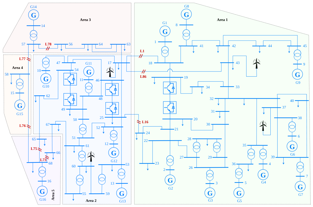
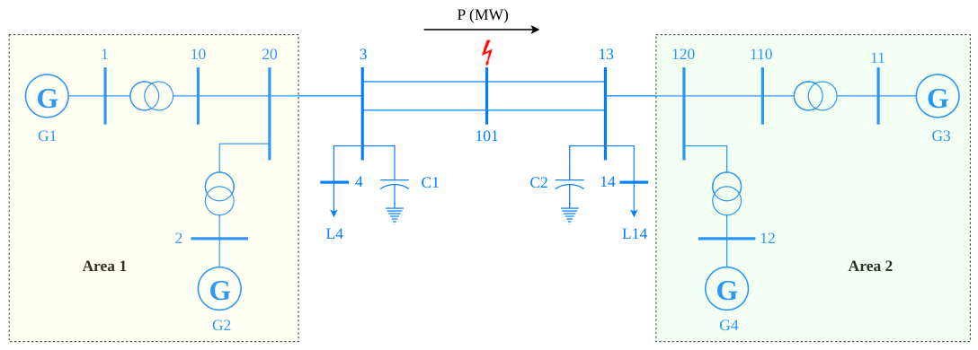
The proposed methodology is evaluated on the two-area Kundur system and the New England–New York power system (NEPS-NYPS) 68-bus system through closed-loop modal displacement and nonlinear post-fault simulations. The Kundur case evaluates coordinated supplementary action through four AVR channels, whereas the NEPS-NYPS case examines the same architecture through sixteen AVR channels and multiple inter-area corridors. Additional scenarios assess the reported sensitivity to communication delays and the modified NEPS-NYPS configuration containing wind power plants and HVDC links. These studies quantify performance under the considered conditions and do not constitute a general robustness guarantee for arbitrary operating-point, topology changes, or communication problems.
The main contributions of this paper are as follows:
A data-assisted dominant modal realization is derived from frequency-response data, impulse-response data, and the retained impulse dynamic subspace, enabling WADC synthesis without requiring a full phenomenological network model.
A discrete-time LQG-WADC is synthesized on the identified dominant modal realization, combining LQR-based damping action with LQE-based reconstruction of reduced coordinates from WAMS measurements.
The proposed controller is validated on the Kundur and NEPS-NYPS benchmarks using modal displacement and nonlinear post-fault simulations, demonstrating coordinated damping through selected AVR supplementary inputs.
The remainder of the paper presents the dominant-modal modeling procedure, the LQG-WADC synthesis, and the modal and nonlinear post-fault validation on the selected benchmarks.
2. Frequency Data-Based Dominant Decomposition Linear Models
This section adopts the power-system linear model derivation by using the dominant mode decomposition framework adapted to multi-machine power networks. The frequency measurements are assembled with direct point-to-point frequency response functions (FRFs), including all spatio-temporal behaviors that are correlated by
where all outputs
and their corresponding inputs
result from applying the fast Fourier transform (fft) to the discrete-time signals
and
, respectively, evaluated at the discrete frequency spectral points
. The excitation signals are defined as chirp functions as in [
13]:
where the amplitude is denoted by
, the lasting time is represented by
T, and
and
are, respectively, the low and high frequencies of the chirp signal. Then, each point in (
1) is mapped into a matrix function
, considering
non-proportional damping modes (
), as follows [
14]:
where
stands for the scaling factor,
represents the mode shapes, and
is the modal participation vectors.
Notice that matrix
for all
and
corresponds to the frequency response functions (FRFs). Then, the impulse response functions (IRFs) are required to assemble the impulse dynamic subspace, as follows [
14]:
where
and
.
2.1. Continuous Time
Dynamic systems can be represented in integral form, avoiding kinematic initial conditions (ICs) and replacing them with dynamic past force evolution
. This forces the system to achieve the actual IC for a fixed
. The mapping of free oscillatory dynamics can be described by the Green function
in the form [
14]
where the system is restricted to its direct dynamics presented by the direct Green function
, and the operator
can be rewritten in a reduced representation by using singular value decomposition (SVD), facilitating the identification of all subsystems in (
6) and assuming a perfect representation of
[
14]:
where
are singular values. The left- and right-singular functions are unitary
,
,
, and
can be derived by taking an appropriate singular set
as
and
. Thus, a direct solution can be rewritten by the introduction of the impulse dynamic subspace based on the
M-left impulse response functions, such that [
14]
This has the following dynamics:
Then, the system matrix can be derived by using the unitary condition of the set of
M left impulse response functions, as
The system matrix in (
10) contains the poles
, with the damped natural angular frequencies
, while
and
(
) are the undamped natural angular frequencies and the damping ratios, respectively.
The solution operator can be derived for the vicinity of the actual state by the impulse dynamic subspace using the evident equity
, leading to [
14]
2.2. Discrete-Time Formulation
Since all frequency response measurements are collected by using a discrete frequency span
(
), where
and the bandwidth is denoted by
, then discretization is performed in the bounded time interval
of the IRF as
(
). Where the number of time intervals is
and the signal length of the discretized IRF is
(if
is in Hz). In this sense, the discretized part of (
6) is expressed as [
14,
15]
In this sense, the so-called Hankel matrix representation of the discrete Green function is [
14]
where the discrete IRF
can simply be compiled by using
ifft on the measured FRFs coordinate-pairwise.
Then, SVD is applied to the direct counterpart of the discrete Green function (
13) as [
14]
where
. Only
M singular values are taken and listed in
. Then, the system matrix can be approximated by using these truncated discrete forms via multiplying the displacement-related
and the velocity-related
singular-IRFs as it was introduced in (
10), that is,
Due to the equivalence between the impulse time coordinates
and
, the velocity-related counterpart of the Green function is computed as
according to (
7). Then, the velocity-related singular-IRFs are derived as
where
and
.
Based on (
11), a discrete map can be derived in the form
where
is a shift matrix shifting the discrete array
by one step (with
). The eigenvalues
of the solution map
are in connection with the poles according to
.
2.3. Applications to Power Systems
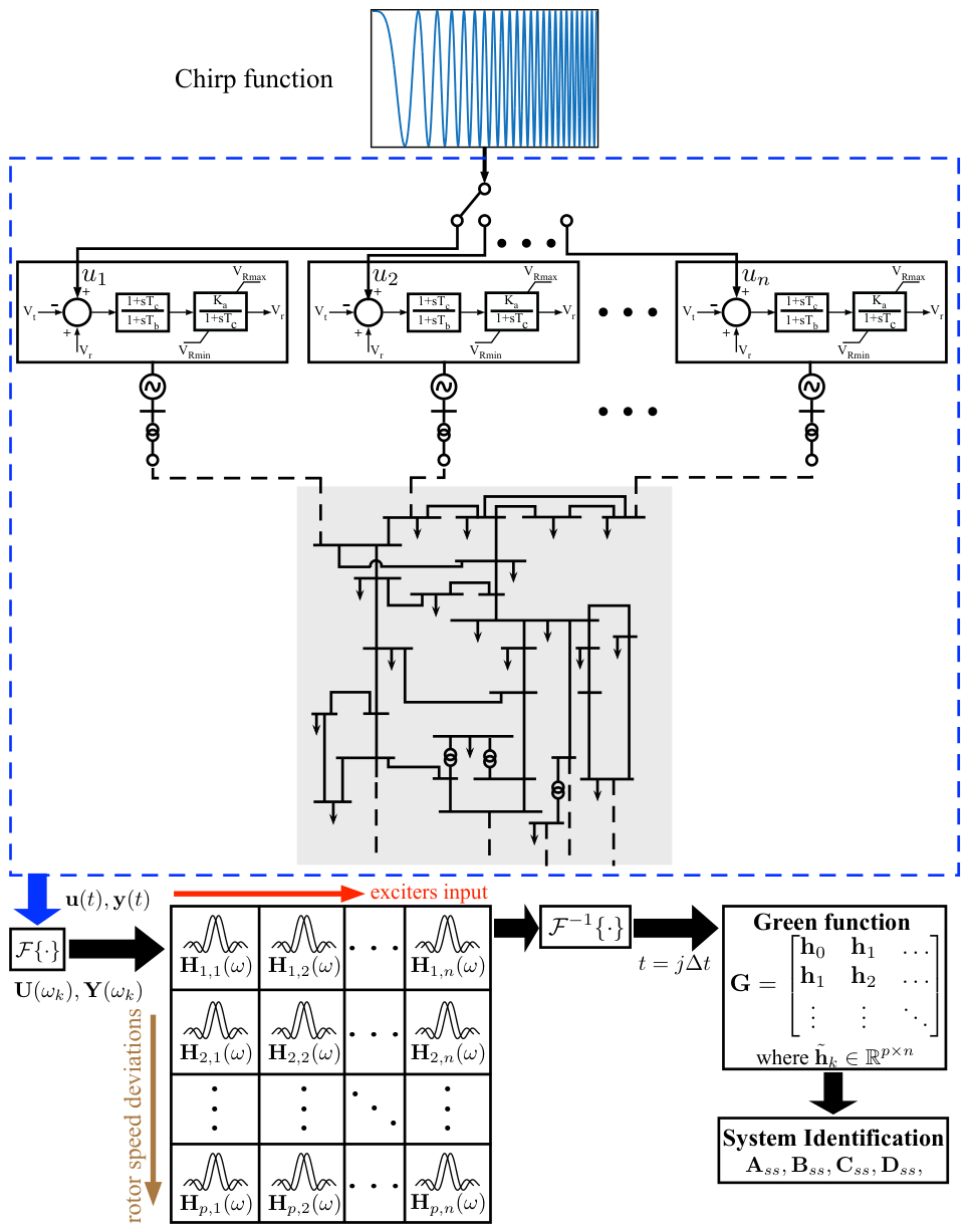
The frequency data-based dominant decomposition for power systems procedure is illustrated in
Figure 1; its implementation is based on the nonlinear simulation environment of the Power System Toolbox (PST) [
16]. The step-by-step execution to gather the multi-input–multi-output (MIMO) data structures is performed as follows:
- 1.
Sequential probing experiments: Rather than exciting all control loops simultaneously, a sequence of independent nonlinear time-domain simulations is carried out column-by-column. For each experiment
i (where
), a logarithmic chirp perturbation signal
is injected exclusively into the reference channel of the
i-th generator’s AVR with
Hz and
Hz, according to (
2). The remaining
excitation inputs are kept inactive.
- 2.
Spatio-temporal data logging: During each simulation run, the dynamic response of the network is recorded over a transient window of to ensure that the electromechanical transient behavior is fully captured. The spatiotemporal output variables, corresponding to the p rotor speed deviations (), are collected and stored. This creates an experimental output data packet associated with the i-th input channel.
- 3.
MIMO data assembly: Once the n sequential simulation runs are completed, the raw time-domain signals are compiled into the global data structures and . These arrays organize the input–output cross-correlations, establishing the definitive link between the nonlinear multi-machine simulation time series and the discrete frequency-domain estimation block () via the fft described in the previous section.
- 4.
IRF computation via IFFT: To isolate the pure impulse dynamics required by the realization algorithm, the ifft is applied to the estimated frequency response matrix . This mathematical operation effectively decouples the nonlinear operational effects of the original chirp signal, mapping the system response back into a clean, time-domain MIMO IRF matrix .
- 5.
Discrete-time Green function assembly: The continuous-time or densely sampled IRF are subsequently re-sampled at a lower rate () tailored for electromechanical oscillation analysis. These discrete parameter blocks () are then systematically and recursively stacked into the so-called Hankel matrix representation of the Green function.
- 6.
System identification (): Finally, the matrix is factored through a singular value decomposition of rank r. The dominant left and right singular vectors are used to compute the discrete-time matrices .
Figure 1.
Flowchart of the DMD-assisted linear models for power systems.
Figure 1.
Flowchart of the DMD-assisted linear models for power systems.
3. LQG-Based Wide-Area Damping Control Design on the DMD-Identified Model
This section presents the wide-area damping controller synthesized from the reduced model obtained in
Section 2. In this paper, DMD refers to the dominant modal decomposition constructed from FRFs, IRFs, and the retained impulse dynamic subspace. It is not used here as a generic snapshot-only dynamic mode decomposition algorithm. This distinction is relevant because the control-oriented realization used below is obtained from the reduced impulse-dynamic coordinates
, not from a snapshot regression operator.
The controller is formulated in discrete time because the identified model is a sampled-data realization and the WADC command is updated at the sampling period . Under the identified linear model and the selected quadratic weights, the linear quadratic Gaussian controller provides an optimal output-feedback law for the adopted stochastic linear-quadratic problem. Its damping effectiveness under nonlinear post-fault responses and operating changes is assessed through time-domain simulations.
For clarity, the LQR, LQE, and LQG have distinct but complementary roles in the proposed controller. The linear quadratic regulator (LQR) is a state-feedback control law that determines the gain K by minimizing a quadratic cost defined by the state and control weighting matrices Q and R, respectively. The linear quadratic estimator (LQE), implemented as a steady-state Kalman estimator, reconstructs the unmeasured reduced state from the available WAMS measurements and determines the estimator gain based on the process- and measurement-noise covariance matrices W and V. The linear quadratic Gaussian (LQG) controller combines these two components through the separation principle: the LQR computes the damping action using the state estimate supplied by the LQE, resulting in the output-feedback law . Thus, the LQR performs optimal regulation, the LQE performs state estimation, and the LQG denotes their integrated output-feedback implementation.
3.1. Control-Oriented Dominant Modal Realization
The solution map
obtained in
Section 2 is an autonomous state-transition operator. To avoid conflict with the control-input matrix
, this section denotes the same operator as
. Hence,
and
.
The reduced realization is expressed in deviation variables around the pre-disturbance operating point, namely,
,
, and
. The deviation symbol is omitted hereafter for compactness. The control-oriented model is
where
is the retained dominant-modal state,
contains the supplementary AVR inputs, and
contains the WAMS measurements used by the estimator. Therefore,
,
, and
. The stochastic terms satisfy
,
, and
.
The input matrix
is not inferred from the autonomous solution map
. It is obtained from the same input–output frequency responses
used in
Section 2, where each supplementary AVR probing signal defines one control input channel. For the
i-th AVR channel, the sampled impulse-response vector is defined as
,
, where
denotes the column of the FRF matrix associated with the
i-th supplementary AVR perturbation and
is the full sampled response vector at the
ℓ-th sampling instant.
The reduced input direction associated with this channel is obtained by projecting the input-induced response onto the retained impulse dynamic subspace:
Here,
is the retained sampled dominant-modal basis,
r is the reduced model order, and
is the dimension of the full sampled response vector. Equation (
19) uses the first discrete Markov parameter of each identified AVR-to-output channel. If a delayed or finite-window Markov representation is used in the implementation,
is replaced by the corresponding input-delay-consistent response vector before projection. This construction ensures that the columns of
represent the dynamic effect of the supplementary AVR inputs in the reduced dominant-modal coordinates, rather than a purely topological incidence relation. The output matrix is obtained as
, where
is the measurement-selection matrix associated with the WAMS channels used by the estimator. Since the supplementary AVR signal acts through the exciter and generator dynamics, no direct algebraic feedthrough from the WADC input to the selected WAMS outputs is considered at the adopted sampling period.
where
denotes the set of generators whose automatic voltage regulators receive supplementary WADC commands, and
. In the implemented benchmarks,
for the Kundur system and
for the NEPS-NYPS system. The measured vector used by the estimator is selected from the available WAMS channels. For the two-area Kundur system, these channels can include monitored tie-line active-power deviations and inter-area speed differences.
where
denotes the set of monitored tie-line power, speed-difference, frequency, or voltage channels retained for damping assessment. The estimator input is
, where
denotes the available monitored-channel set and
is the binary selection matrix defining the channels supplied to the implemented LQE. Speed or frequency-difference channels may be appended when they are part of the implemented measurement set and improve observability of the target inter-area modes.
The vector contains the measured channels used by the estimator, contains the variables weighted in the LQR cost, and contains the outputs used for time-domain validation. These sets may overlap, but they need not be identical.
To avoid unit-dependent tuning, the variables are normalized as
,
, and
, where
,
, and
are diagonal scaling matrices. The entries of
are selected from the admissible supplementary AVR limits, and the entries of
are selected from representative magnitudes of the measured WAMS channels. The normalized realization is
with
,
, and
. The scaling matrices are fixed before solving the Riccati equations and are kept unchanged during each nonlinear validation case.
3.2. LQR-Based Damping Synthesis
The regulator computes the supplementary damping action by minimizing
where
penalizes the target oscillatory content and
penalizes the supplementary AVR effort. The full-state LQR law is
. In the implemented LQG controller,
is replaced by its LQE estimate. The gain is
and
is the stabilizing solution of
The LQR solution is retained only if
is stabilizable and
is detectable. The weighting matrix
Q is connected to the damping objective through the performance output
:
where
weights the selected oscillatory variables and
regularizes non-penalized reduced directions. The vector
may include inter-area speed differences, center-of-inertia frequency deviations, or active-power deviations across critical tie-lines. The effort matrix is selected as
, where
penalizes the
i-th supplementary AVR channel. The LQR determines the full-state damping gain
K, whereas the LQE supplies the reduced-state estimate required to implement the output-feedback LQG law
.
3.3. LQE-Based Wide-Area State Reconstruction
The retained dominant-modal state is not directly measured. A steady-state Kalman estimator estimates its reduced coordinates from the selected PMU/WAMS signals. To avoid ambiguity between predictor–corrector notation and stationary estimator equations, the LQE is written in observer form:
where
is the steady-state estimator gain. Let
be the stationary estimation-error covariance associated with the observer form in (
27). It is obtained from
and the estimator gain is
The estimator is retained only if
is detectable and
is stabilizable. The matrix
W represents uncertainty in the dominant-modal model and neglected high-order dynamics, while
V represents PMU/WAMS measurement uncertainty.
3.4. Integrated Dominant Modal LQG-WADC Implementation
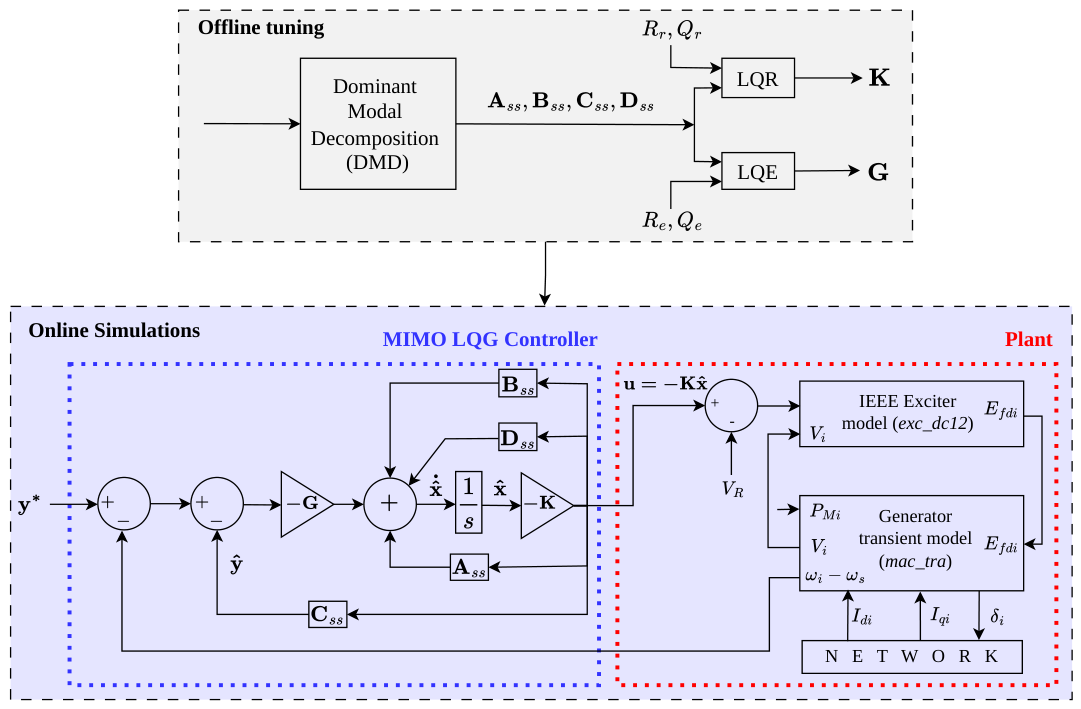
The nominal LQG gains are synthesized from the delay-free reduced realization. Communication delays are subsequently introduced in the WAMS measurement path during nonlinear validation. Hence, the reported delay cases quantify sensitivity of the nominal controller rather than the performance of a delay-compensated LQG design. The LQG controller combines the regulator and estimator through the separation principle. Since the actual reduced state is not measured, the implemented control law is
Before being applied to the excitation system, each physical channel is limited as
,
. The command injected into the
i-th AVR is
This equation defines the physical interface between the dominant-modal LQG controller and the nonlinear power-system model.
For the unsaturated linear reduced model, the regulator and estimator poles are
The LQG realization is accepted only if
For complex-conjugate regulator poles associated with electromechanical modes, the equivalent damping ratio and modal frequency are
In the simulations reported in this work, is used according to the electromechanical frequency range targeted by the WADC. The controller is not intended to act during the fault inception itself, but to damp the post-fault inter-area oscillatory response after fault clearing.
The admissibility check has two levels. The first level verifies modal displacement and internal stability in the reduced linear model. The second level verifies bounded AVR commands and reduced post-fault oscillations in nonlinear time-domain simulations. The controller tuning
is retained when
Here, is the set of targeted electromechanical modes, and is the set of monitored critical outputs. For the Kundur system, includes the monitored tie-line power flows and generator-speed differences. For the NEPS-NYPS system, includes the critical inter-area corridors selected from . Among the admissible candidates, the selected controller is the one with the largest admissible R-scaling, or equivalently the smallest peak supplementary AVR command, while satisfying .
The dimensions
r,
m, and
p, together with the selected actuation channels, WAMS measurements, scaling matrices, and LQG weights, are fixed for each benchmark before solving the Riccati equations. The resulting WADC in
Figure 2 follows the sequence: dominant-modal model identification, projection of AVR and WAMS channels onto the retained dynamic subspace, normalization, LQR/LQE synthesis, supplementary AVR command generation, and validation through modal displacement and nonlinear post-fault simulations.
6. Conclusions
By projecting the AVR excitation channels and output measurements onto the retained impulse-dynamic subspace, the proposed identification technique successfully bypasses the requirement for full dynamic network parameters while preserving an exact physical mapping of the dominant oscillatory modes. Furthermore, comparative evaluations against SSA demonstrate that this data-assisted realization captures inter-area and local modal frequencies and damping ratios with higher precision, while accurately reconstructing the mode shapes and spatial dynamic activity across the power grid. As a result, the extracted subspace provides a clear, control-oriented state-space model directly from multichannel WAMS measurements.
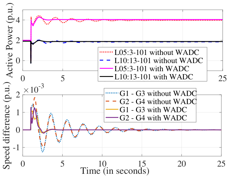
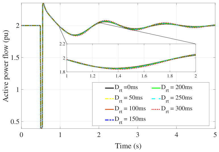
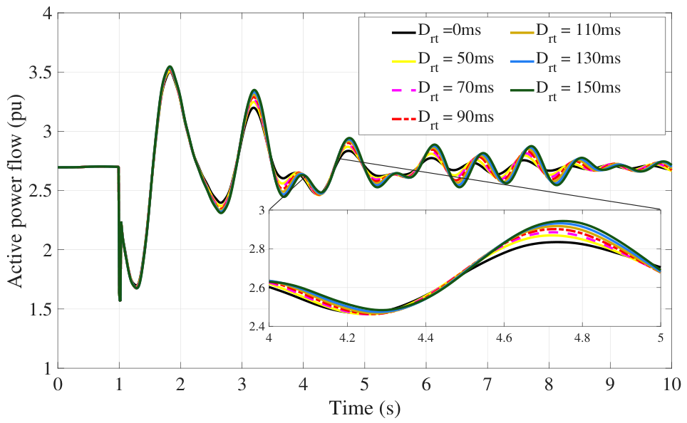
The attained results demonstrate that the proposed dominant modal realization supports coordinated wide-area damping synthesis in addition to modal assessment. In the Kundur system, the discrete-time LQG controller uses four supplementary AVR channels to attenuate the post-fault tie-line power and inter-area speed responses, with the reported power-flow oscillations damped in less than . The same architecture is extended to the NEPS-NYPS benchmark through sixteen AVR channels and multiple monitored inter-area corridors. Together, the modal-displacement results and nonlinear fault simulations indicate that the FRF/IRF-derived dominant subspace captures the control-relevant dynamics required for output-feedback WADC synthesis in an interpretable control-oriented representation. The Kundur latency study further shows that the reported line-flow response remains qualitatively preserved for communication delays from 50 to . These results demonstrate that the proposed DMD–LQG framework provides a transparent measurement-derived route for coordinated AVR-based damping, while broader validation under operating-point uncertainty, packet losses, and larger communication disturbances remains necessary.
Even with the addition of rotor-angle signal latency in the synchronous generators, the WADC implemented in both systems still dampens oscillations, proving suitable performance under unfavorable operating conditions. However, it is important to consider that the good response of this control to delay is largely due to the accurate identification of the oscillatory modes using the DMD method.
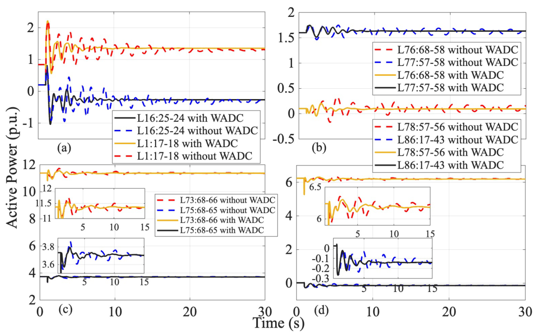
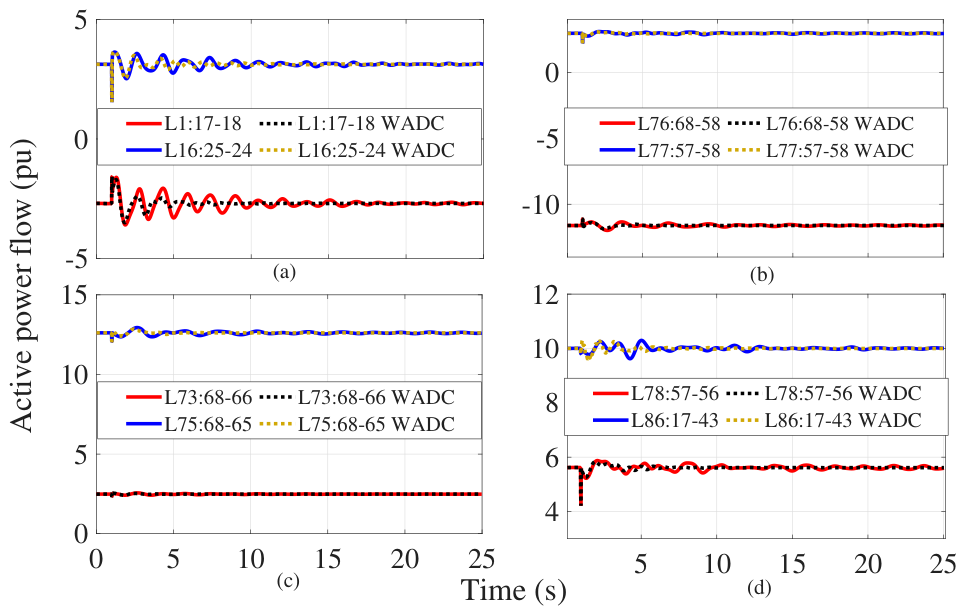
In the second scenario of the NEPS-NYPS, which adds wind power plants and an HVDC line, the WADC strategy enhances the system’s ability to respond to external disturbances. This improvement occurs because the initial identification detects the inter-area modes that influence the system; thus, even with these mitigating elements in place, the control effectively dampens oscillations by reducing the settling time and overshoot magnitude.




 ,
,