Research on Single-Ended Protection for Multi-Terminal Flexible DC Lines Based on Line-Mode Reverse Traveling-Wave Covariance

Abstract

Multi-terminal HVDC transmission lines contain a T-zone, where no explicit line boundary element exists. Conventional traveling-wave (TW) protection schemes mainly identify faults by utilizing the attenuation characteristics of TWs caused by transmission lines and boundary elements. Therefore, their performance is sensitive to transition resistance and sampling frequency, and they cannot be directly applied to fault identification in the T-zone. To address this issue, this paper proposes a single-ended directional protection scheme based on the normalized covariance of line-mode backward TWs. The proposed method constructs the protection criterion according to the overall waveform variation in line-mode backward TWs. It does not rely on boundary-effect-induced wave attenuation or the extraction of specific high- or low-frequency components. Fault regions are identified using only local measurements collected by the protection devices installed on both sides of the T-zone, and the fault pole is determined by the bipolar voltage ratio. A ±500 kV three-terminal MMC-based multi-terminal DC system is established in PSCAD to evaluate the proposed scheme. Simulation results show that the proposed method identifies the fault region within a 0.5 ms data window. It can tolerate transition resistances up to 300 Ω and 40 dB Gaussian white noise. The proposed scheme features fast operation, low computational complexity, and high robustness.

1. Introduction

Owing to the uneven distribution of energy resources and the long transmission distance between generation sites and load centers, high-voltage direct current (HVDC) transmission has become an important technology for long-distance bulk power transfer [1,2,3]. Conventional line-commutated converter (LCC)-HVDC systems employ semi-controlled power electronic devices that can only control the turn-on process. As a result, they are susceptible to commutation failures when operating under weak AC grid conditions, where even minor disturbances may threaten the secure operation of the power system [4,5].

In contrast, voltage source converter (VSC)-HVDC technology eliminates the risk of commutation failure and provides flexible and independent control of active and reactive power [6,7]. Owing to these advantages, VSC-HVDC has become a preferred solution for integrating large-scale renewable energy sources and developing multi-terminal DC grids, attracting increasing attention in recent years [8,9].

HVDC transmission line protection has been generally classified into two categories based on the data acquisition method: unit protection and non-unit protection [10]. Unit protection relies on communication channels to exchange data between protection devices at both ends of the line. Typical methods include current differential protection [11], voltage differential protection [12], and impedance differential protection [13]. Although these methods can accurately identify internal faults within the protection zone, they strictly require remote communication and precise time synchronization. Consequently, issues such as communication latency, stringent synchronization requirements, and high engineering costs inevitably arise, which limit their application in ultra-high-speed protection. In contrast, non-unit protection identifies faults utilizing only local measurements without the need for remote communication or time synchronization [7]. Due to its rapid operating speed and simple implementation, non-unit protection has become a vital research direction in flexible HVDC protection. Depending on the construction of the protection criterion, existing non-unit protection methods can be categorized into the following three types:

(1)

Protection Methods Based on DC Reactor (DCR) Voltage

These methods primarily utilize the voltage across the DC reactor (DCR) or the voltage difference between the positive and negative poles to construct protection criteria [14], thereby achieving internal and external fault identification. However, because high-resistance faults generate weak transient characteristics, the capability of these methods to detect high-resistance faults is limited. Furthermore, they exhibit poor adaptability to certain fault types.

(2)

Protection Methods Based on Time-Domain TWs

These methods construct protection criteria by utilizing the ratio of change in voltage (ROCOV), the rate of change in current (ROCOC), or the characteristics of the initial TW front, offering advantages such as rapid operating speed and the absence of communication requirements [15]. For instance, Reference [16] utilizes the wavelet transform modulus maxima to extract the polarities of the initial voltage and current TWs to achieve fault direction discrimination.

(3)

Protection Methods Based on Time-Frequency Analysis

These methods mainly employ signal processing techniques—such as the wavelet transform (WT), short-time Fourier transform (STFT), Hilbert–Huang transform (HHT), and mathematical morphological gradient (MMG)—to extract high-frequency features of fault transients, thereby enhancing the fault detection capability under high transition resistance and improving noise immunity. Nevertheless, these methods typically depend on complex signal processing algorithms, impose stringent requirements on the sampling frequency (with some methods reaching the megahertz level), and require significant computational overhead, which places certain constraints on their real-time engineering applications [17].

In summary, most existing non-unit protection methods rely heavily on the initial TW front, high-frequency transient components, or specific frequency band features, thereby imposing stringent requirements on the sampling frequency, noise immunity, and signal processing algorithms. When these methods are applied to multi-terminal flexible HVDC transmission systems embedding T-junctions, the lack of distinct boundary characteristics in the T-zone creates a significant challenge. Specifically, when fault TWs propagate near the T-zone, they fail to produce identifiable differences in high-frequency components or initial TW fronts. Consequently, traditional protection methods dependent on frequency or wavefront features face inherent limitations. Therefore, it is essential to develop a novel protection scheme that operates without the need to extract specific frequency components and remains independent of differences in TW fronts.

To address the challenge of fault zone identification in multi-terminal flexible HVDC transmission lines with T-connections, this paper proposes a single-ended ultra-fast protection scheme based on the normalized covariance of line-mode backward TWs. Due to the absence of DC reactors on both sides of the T-zone, traditional protection methods relying on reactor voltage or initial TW front features are prone to failure. To overcome this limitation, the proposed scheme utilizes the overall variation trend of the line-mode backward TWs within a short 0.5 ms data window to construct the protection criterion, completely avoiding cumbersome time-frequency transformations and feature extraction steps. Furthermore, by introducing a normalized covariance algorithm, the scheme eliminates the interference of transition resistance on TW amplitudes, achieving ultra-fast protection that operates solely on local single-ended measurements without communication delays.

The main contributions and novelties of this study are summarized as follows:

(1)

To tackle the issue where traditional methods fail to distinguish faults located on the left, right, or inside the T-zone due to the lack of DC reactors and noticeable high-frequency attenuation or TW front discrepancies, the proposed scheme relies on the overall backward TW trend over a 0.5 ms window. By eliminating dependence on high-frequency features and initial wavefronts, it not only accurately identifies T-zone faults but also significantly relaxes sampling rate requirements (operating effectively even at 50 kHz, and withstanding severe Gaussian white noise of up to 40 dB).

(2)

Unlike traditional covariance algorithms or magnitude-dependent protection schemes that are susceptible to transition resistance, the introduced normalization completely removes amplitude discrepancies, allowing the criterion to focus strictly on overall waveform trends. The algorithm operates reliably under high transition resistances of up to 300 Ω, with a simple mathematical formulation and low computational overhead that ensure easy engineering implementation.

(3)

Ultra-Fast Single-Ended Operation Performance: Operating exclusively on local single-ended electrical quantities, the scheme entirely eliminates communication latency. With minimal computational complexity, the calculation delay is practically negligible, accomplishing the full process from TW sampling to trip signal issuance within just 0.5 ms to deliver ultra-fast protection performance.

2. Analysis of Fault Traveling-Wave Propagation Characteristics

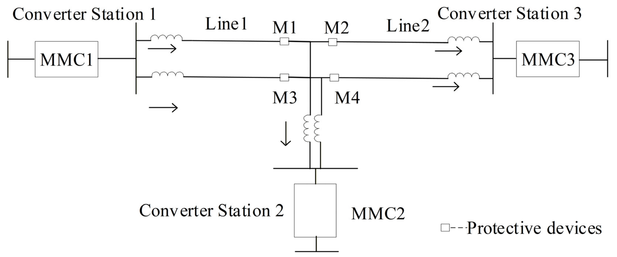
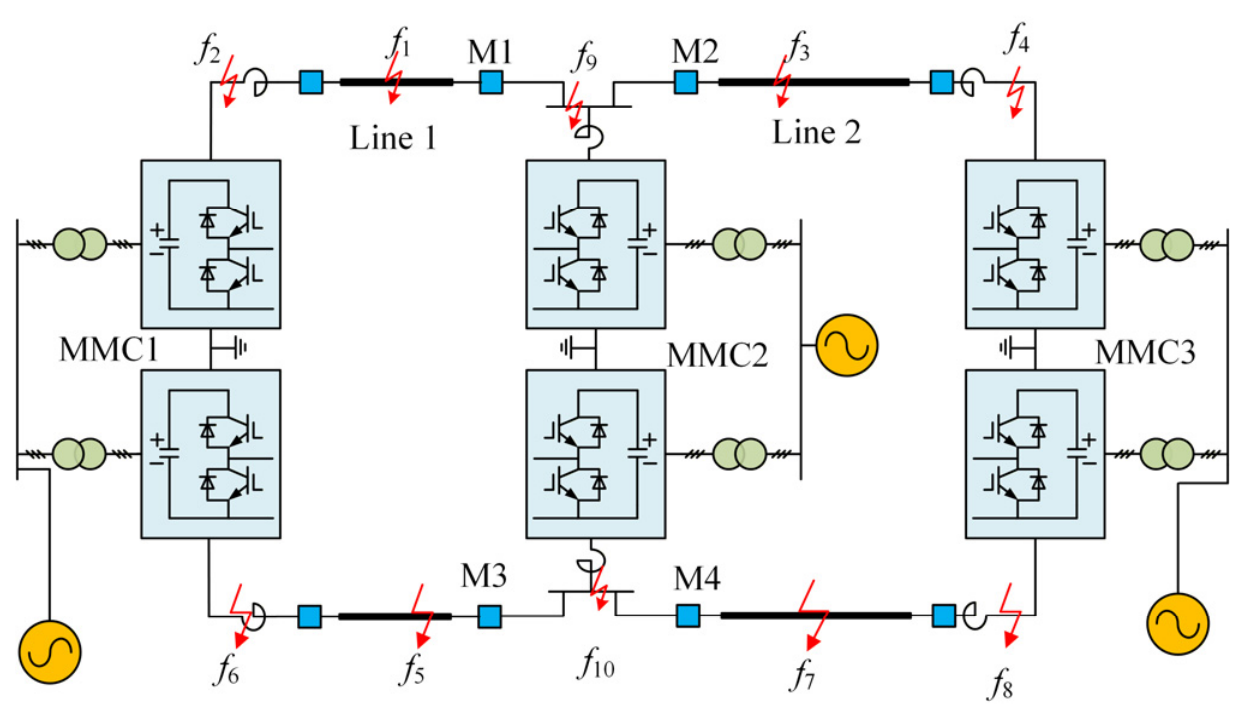
Figure 1 illustrates the topology of a multi-terminal flexible HVDC transmission system. In this configuration, Station 1 (MMC 1) functions as the sending end (rectifier station), whereas Stations 2 (MMC 2) and 3 (MMC 3) operate as the receiving ends (inverter stations), with a rated DC voltage level of $\pm$500 kV. Current-limiting DCRs are installed at the sending end of Line 1, the receiving end of Line 2, and the export terminal of MMC 2. Consequently, MMC 2, together with Line 1 and Line 2, forms a T-junction topology. The three MMC-based stations are interconnected through Line 1, the T-connected bus bar, and Line 2 to constitute the multi-terminal flexible HVDC system. Regarding the configuration of the protection system, the protection devices M1 and M3 are deployed at the positive and negative terminals at the end of Line 1, respectively, to protect the entire length of Line 1. Similarly, the protection devices M2 and M4 are positioned at the positive and negative terminals at the beginning of Line 2, respectively, to provide full-length protection for Line 2.

2.1. TW Propagation Characteristics of Internal T-Zone Faults and Line Faults

2.1.1. Fault Traveling-Wave Characteristics Along Line 1 on the Left Side of the T-Zone

Taking a positive-pole fault as an illustrative example, when a fault occurs on the transmission line, the voltage at the fault point drops abruptly. This phenomenon is equivalent to superimposing a negative step signal at the fault point. Consequently, the initial fault line-mode voltage traveling wave (TW) can be expressed as follows:

$$u_{\mathrm{L}}=-{\displaystyle \frac{\sqrt{2}{U}_{\mathrm{dc}}{Z}_{\mathrm{L}}}{Z_{\mathrm{G}}+Z_{\mathrm{L}}+4R_{\mathrm{f}}}}$$

(1)

where $u_{\mathrm{L}}$ represents the initial line-mode fault voltage TW; $U_{\mathrm{dc}}$ denotes the DC voltage amplitude during steady-state operation; $Z_{\mathrm{G}}$ and $Z_{\mathrm{L}}$ are the earth-mode and line-mode wave impedances, respectively; and $R_{\mathrm{f}}$ represents the transition resistance.

(1)

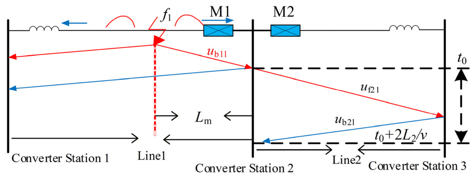
The traveling-wave reflection and transmission process for a fault on Line 1 on the left side of the T-zone is illustrated in Figure 2.

Specifically, $t_0$ represents the arrival time of the initial fault backward TW detected by device M1. Within the time window $\left[t_0,t_0+2L_2/v\right]$, the line-mode backward TW predominantly captured by protection device M1 is $u_{\mathrm{b}11\mathrm{L}}$. The line-mode backward TWs reflected from the bus bar are neglected due to their significant attenuation caused by time propagation delay, line attenuation, and the reflection coefficient, making them considerably smaller than the initial fault line-mode backward TW. Consequently, the time-domain expression of the line-mode backward TW detected by protection device M1 within this specified time window can be derived as follows:

$$\left\{\begin{array}{l}{u}_{\mathrm{b}11\mathrm{L}}=u_{\mathrm{L}}·A(t)=-{\displaystyle \frac{\sqrt{2}{U}_{\mathrm{dc}}{Z}_{\mathrm{L}}}{Z_{\mathrm{L}}+Z_{\mathrm{G}}+4R_{\mathrm{f}}}}·A(t)\\ A(t)=(1-kx)·{\displaystyle \frac{1}{\tau x}}{\mathrm{e}}^{-{\displaystyle \frac{t-x/v}{\tau x}}}\end{array}\right.$$

(2)

where $u_{\mathrm{b}11\mathrm{L}}$ represents the line-mode backward TW passing through protection device M1 within the specified time window; $A\left(t\right)$ denotes the propagation function of the TW along the transmission line; $v$ is the propagation velocity of the line-mode TW; $k$ and $\tau$ represent the attenuation and dispersion coefficients of the line-mode component, respectively; and $x$ denotes the distance from the fault point to protection device M1.

When a fault occurs along the Line 1 on the left side of the T-zone, the variation in the line-mode backward TW detected by protection device M1 is illustrated in Figure 3.

As can be observed from Figure 3, when a fault occurs along Line 1, the backward TW detected by protection device M1 within the time window $\left[t_0,t_0+2L_2/v\right]$ exhibits a rapidly declining trend.

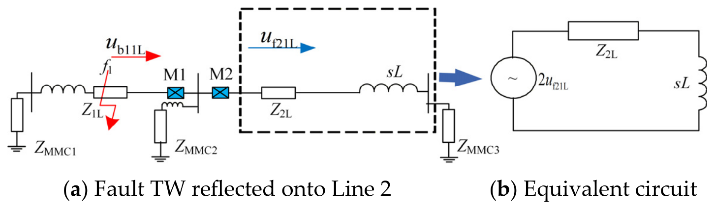
The fault equivalent circuit for a fault on the left side of the T-zone is illustrated in Figure 4. After the fault occurs on the left side of the T-zone, $u_{\mathrm{b}11\mathrm{L}}$ refracts through the T-zone into Line 2, yielding $u_{f21\mathrm{L}}$. As $u_{\mathrm{f}21\mathrm{L}}$ propagates through Line 2 and the DCR, the equivalent circuit is established as shown in Figure 4b.

Based on the equivalent voltage circuit shown in Figure 4b, the corresponding differential equation is established. By combining the propagation path of the initial fault traveling wave shown in Figure 4a with the relationship that the reflected wave equals the transmitted wave minus the incident wave, the line-mode backward traveling wave detected by M2 can be expressed as follows:

$$\left\{\begin{array}{l}L{\displaystyle \frac{\mathrm{d}i}{\mathrm{d}t}}+Z_{2\mathrm{L}}·i=2u_{\mathrm{f}21\mathrm{L}}\\ u_{\mathrm{f}21\mathrm{L}}=u_{\mathrm{L}}·A(t)·\beta \\ u_{\mathrm{b}21\mathrm{L}}=2u_{\mathrm{f}21\mathrm{L}}·{\mathrm{e}}^{-{\displaystyle \frac{Z_{2\mathrm{L}}}{L}}t}-u_{\mathrm{f}21\mathrm{L}}\end{array}\right.$$

(3)

where $Z_{2\mathrm{L}}$ represents the equivalent line-mode wave impedance of Line 2, and $u_{\mathrm{f}21\mathrm{L}}$ denotes the fault line-mode forward TW refracted into Line 2, and $\beta$ denotes the refraction coefficient at the bus bar of the $\mathrm{T}\text{-}\mathrm{zone}$, and $u_{\mathrm{b}21\mathrm{L}}$ represents the line-mode backward TW reflected from the boundary reactor of MMC 3.

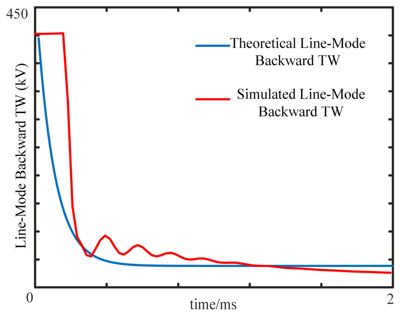
The simulated and theoretical waveforms of the $u_{\mathrm{b}21\mathrm{L}}$ are illustrated in Figure 5.

As can be derived from (3), the line-mode backward TW $u_{\mathrm{b}21\mathrm{L}}$ reflected by the reactor contains two polarities [18]: one possesses the same polarity as the initial incident TW, while the other exhibits the opposite polarity to the initial incident TW. Due to the influence of the line frequency-dependent parameters, the TW component with the same polarity as the initial TW has a smaller amplitude, a shorter rise time, and contains more high-frequency components, leading to significant attenuation during transmission along the line. Conversely, the component with the opposite polarity to the initial TW possesses a larger amplitude and still varies exponentially. Consequently, the waveform in Figure 5 exhibits a trend of initially declining and subsequently rising.

In summary, when a fault occurs outside the $\mathrm{T}\text{-}\mathrm{zone}$ on the left side, the line-mode backward TW detected by protection device M1 exhibits a declining trend, whereas the line-mode backward TW detected by protection device M2 displays a trend of initially declining and subsequently rising. The aforementioned fault analysis process is equally applicable to both positive-pole and negative-pole faults.

2.1.2. Fault Traveling-Wave Characteristics Along Line 2 on the Right Side of the T-Zone

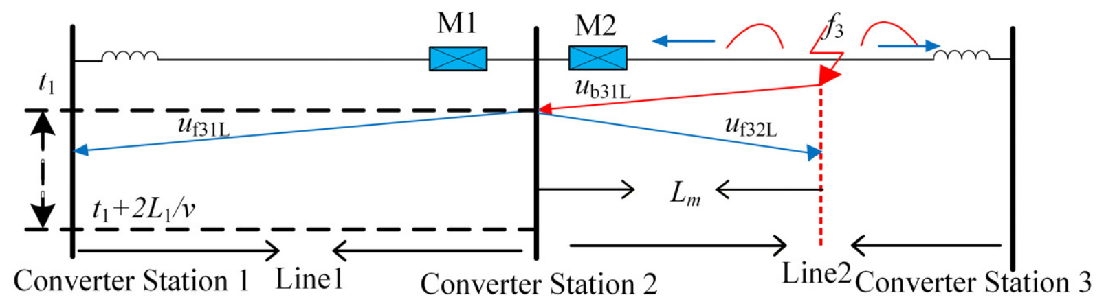
When a fault occurs along Line 2 on the right side of the T-zone, the reflection process of the fault TW is shown in Figure 6.

As illustrated in Figure 6, when a fault occurs on the right side of the $\mathrm{T}\text{-}\mathrm{zone}$, $t_1$ represents the arrival time of the fault TW detected by device M2. Within the time window $t_1,t_1+2L_1/v$, the line-mode backward TW predominantly captured by protection device M2 is $u_{\mathrm{b}31\mathrm{L}}$.

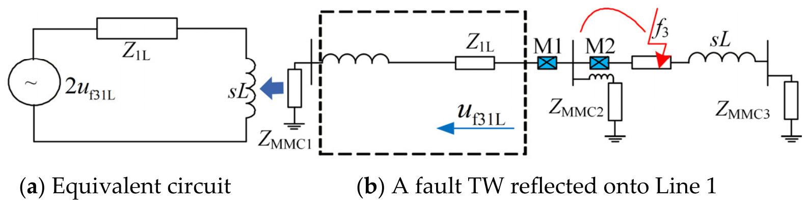
Combining with Figure 6, after a fault occurs on Line 2, the fault TW $u_{\mathrm{f}31\mathrm{L}}$ propagates through Line 1 and the DCR, where $Z_{1\mathrm{L}}$ represents the equivalent line-mode wave impedance of Line 1, and its equivalent circuit is established as shown in Figure 7.

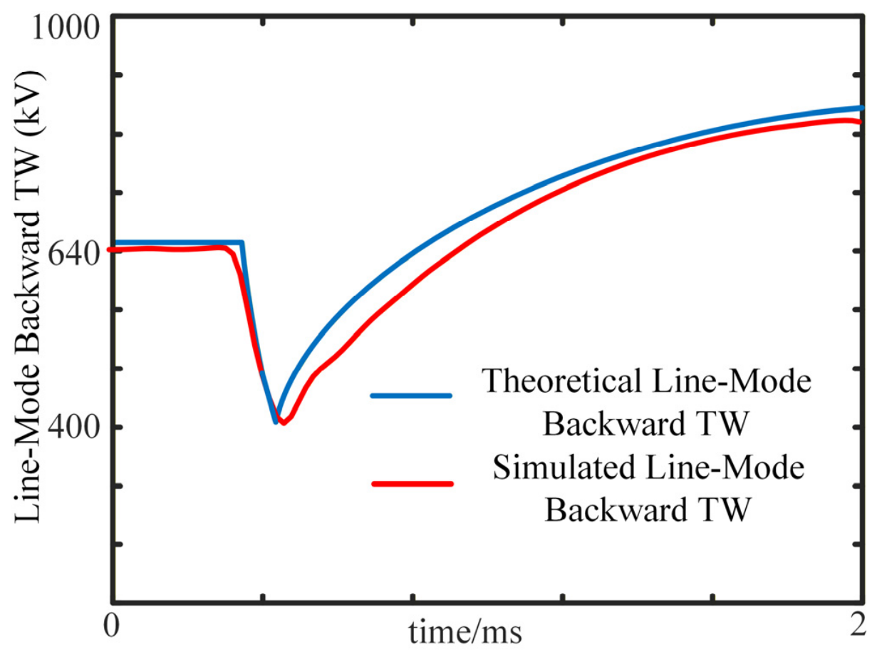
Based on the equivalent circuit shown in Figure 7a, the differential equation for the voltage loop can be formulated. By combining this equation with the relationship between the reflection and transmission coefficients, the expressions for the line-mode backward TWs detected by devices M1 and M2 can be derived.

$$\left\{\begin{array}{l}L{\displaystyle \frac{\mathrm{d}i}{\mathrm{d}t}}+Z_{1\mathrm{L}}·i=2u_{\mathrm{f}31\mathrm{L}}\\ u_{\mathrm{b}32\mathrm{L}}=L{\displaystyle \frac{\mathrm{d}i}{\mathrm{d}t}}-u_{\mathrm{f}31\mathrm{L}}=2u_{\mathrm{f}31\mathrm{L}}·{\mathrm{e}}^{-{\displaystyle \frac{Z_{1\mathrm{L}}}{L}}t}-u_{\mathrm{f}31\mathrm{L}}\\ u_{\mathrm{b}31\mathrm{L}}=u_{\mathrm{L}}·A(t)·\beta \end{array}\right.$$

(4)

where $u_{\mathrm{f}31\mathrm{L}}$ represents the fault line-mode forward TW refracted into Line 1; $u_{\mathrm{b}32\mathrm{L}}$ denotes the line-mode backward TW reflected from the boundary reactor of MMC 1; $u_{\mathrm{b}31\mathrm{L}}$ represents the initial fault line-mode backward TW passing through protection device M2 within the specified time window; and $u_{\mathrm{L}}$ denotes the initial fault line-mode TW.

Due to the structural similarity between $u_{\mathrm{b}11\mathrm{L}}$ in (2) and $u_{\mathrm{b}31\mathrm{L}}$ in (4), it can be inferred that the waveform of $u_{\mathrm{b}31\mathrm{L}}$ also exhibits a declining trend. Similarly, since the structure of $u_{\mathrm{b}21\mathrm{L}}$ in (3) is similar to that of $u_{\mathrm{b}32\mathrm{L}}$ in (4), the waveform of $u_{\mathrm{b}32\mathrm{L}}$ can be considered to display a trend of initially declining and subsequently rising.

2.1.3. Fault Traveling-Wave Characteristics of Faults Within the T-Zone

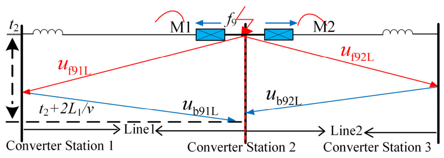
Taking a positive-pole internal fault inside the $\mathrm{T}\text{-}\mathrm{zone}$ as an illustrative example, the analysis process for a negative-pole internal fault inside the $\mathrm{T}\text{-}\mathrm{zone}$ is similar. When an internal fault occurs inside the $\mathrm{T}\text{-}\mathrm{zone}$, the reflection and transmission process of the fault TWs is illustrated in Figure 8.

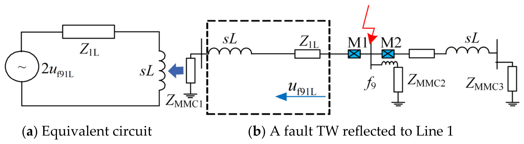
For protection device M1, an internal fault inside the $\mathrm{T}\text{-}\mathrm{zone}$ is equivalent to a fault occurring on the right side of M1. Consequently, the fault backward TW detected by M1 exhibits characteristics similar to those analyzed in Section 2.1.2. For protection device M2, this scenario is equivalent to a fault occurring on the left side of M2, and the fault backward TW detected by M2 is similar to the analysis in Section 2.1.1. Taking protection device M1 as an illustrative example, since M2 follows an identical analysis process, when an internal fault occurs inside the $\mathrm{T}\text{-}\mathrm{zone}$, the fault line-mode TW $u_{\mathrm{f}91\mathrm{L}}$ propagates through Line 1 and the DCR. The corresponding fault equivalent circuit is illustrated in Figure 9.

Based on the equivalent circuit shown in Figure 9a, the differential equation for the voltage loop can be formulated. By combining this equation with the relationship between the reflection and transmission coefficients, the expression for the line-mode backward TW $u_{\mathrm{b}91\mathrm{L}}$ can be derived as follows:

$$\left\{\begin{array}{l}L{\displaystyle \frac{\mathrm{d}i}{\mathrm{d}t}}+Z_{1\mathrm{L}}·i=2u_{\mathrm{f}91\mathrm{L}}\\ u_{\mathrm{b}91\mathrm{L}}=L{\displaystyle \frac{\mathrm{d}i}{\mathrm{d}t}}-u_{\mathrm{f}91\mathrm{L}}=2u_{\mathrm{f}91\mathrm{L}}·{\mathrm{e}}^{-{\displaystyle \frac{Z_{1\mathrm{L}}}{L}}t}-u_{\mathrm{f}91\mathrm{L}}\end{array}\right.$$

(5)

where $u_{\mathrm{f}91\mathrm{L}}$ represents the fault line-mode forward TW propagating to Line 1; and $u_{\mathrm{b}91\mathrm{L}}$ represents the line-mode backward TW reflected by the boundary reactor of MMC 1.

It can be observed that the expression of $u_{\mathrm{b}91\mathrm{L}}$ in (5) is similar to that of $u_{\mathrm{b}21\mathrm{L}}$ in (3). When an internal fault occurs inside the $\mathrm{T}\text{-}\mathrm{zone}$, the line-mode backward TW detected by protection device M1 exhibits a trend of initially declining and subsequently rising. Similarly, the fault TW will also propagate to Line 2 and undergo reflection at the boundary on the side of MMC 3. Consequently, the line-mode backward TW detected by protection device M2 also displays a trend of initially declining and subsequently rising.

2.2. Fault Traveling-Wave Characteristics Outside MMCs

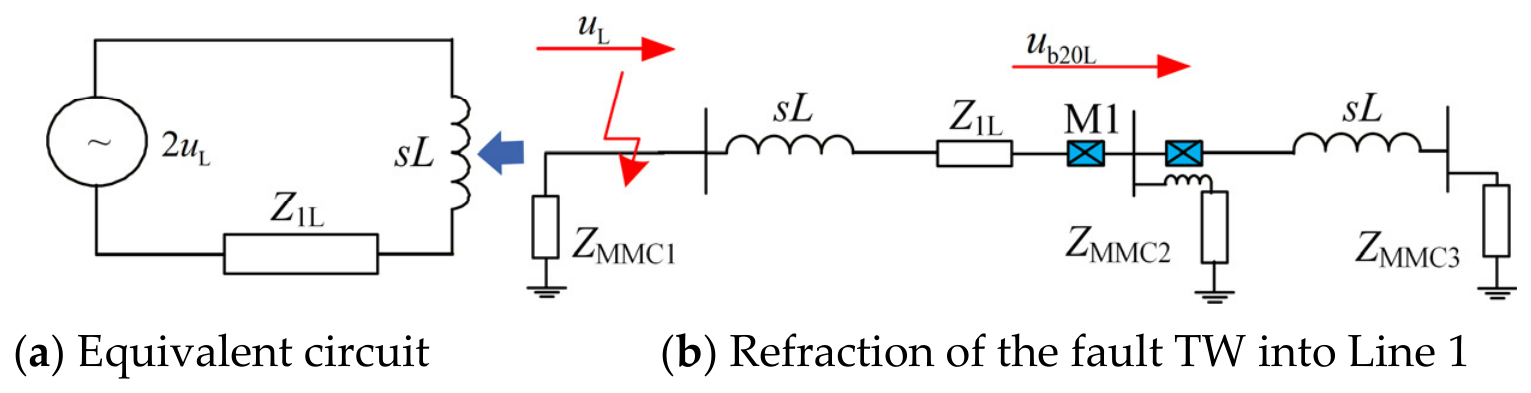
Taking a positive-pole external fault outside $\mathrm{MMC} 1$ as an illustrative example, the analysis process for a negative-pole external fault outside $\mathrm{MMC} 1$ is similar. When an external fault occurs outside $\mathrm{MMC} 1$, the reflection and transmission process of the fault TWs is illustrated in Figure 10.

Based on the equivalent circuit shown in Figure 10b, the differential equation for the loop can be formulated, and the expression for the line-mode backward TW detected by device M1 can be derived as follows in (6):

$$\left\{\begin{array}{l}L{\displaystyle \frac{\mathrm{d}i}{\mathrm{d}t}}+Z_{1\mathrm{L}}·i=2u_{\mathrm{L}}\\ i={\displaystyle \frac{2u_{\mathrm{L}}}{Z_{1\mathrm{L}}}}\times \left({1-\mathrm{e}}^{-{\displaystyle \frac{t}{T}}}\right)\\ u_{\mathrm{b}20\mathrm{L}}=i·Z_{1\mathrm{L}}·A(t)=2u_{\mathrm{L}}·\left({1-\mathrm{e}}^{-{\displaystyle \frac{t}{T}}}\right)·A(t)\end{array}\right.$$

(6)

where $u$ represents the initial fault line-mode backward TW at the side of MMC 1; $Z_{1\mathrm{L}}$ is the equivalent line-mode wave impedance of Line 1; and $T$ denotes the time constant, the magnitude of which is $L/Z_1$.

As can be derived from (6), when an external fault occurs outside MMC 1, the line-mode backward TW $u_{\mathrm{b}20\mathrm{L}}$ detected by protection device M1 is predominantly limited by the exponential attenuation effect of the DCR. Compared with the declining waveform described in (2) under a fault along Line 1 on the left side of the $\mathrm{T}\text{-}\mathrm{zone}$, the waveform of the line-mode backward TW $u_{\mathrm{b}20\mathrm{L}}$ under the external fault is smoother and possesses a smaller amplitude. Similarly, when an external fault occurs on the side of MMC 3, the fault TW propagating to protection device M2 will likewise be affected by the attenuation of the DCR, exhibiting a similar characteristic of smooth variation.

3. Protection Criteria and Protection Scheme

3.1. Start-Up Criterion

The derivative of the DC line-mode voltage is selected as the start-up criterion for the proposed protection scheme, which can be mathematically formulated as [19]:

$$\left|{\displaystyle \frac{\mathrm{d}{u}_1}{\mathrm{d}t}}\right|>\mathsf{\Delta }u$$

(7)

where $u_1$ represents the DC line-mode voltage. The setting value $\Delta u$ is determined based on the maximum voltage gradient under the most severe external fault, while incorporating a sufficient reliability margin to evade measurement errors and high-frequency noise levels [20]. In this paper,$\mathsf{\Delta }u$ is set to 2 kV/0.01 ms.

3.2. Fault Region Identification Criterion

According to the analysis of fault TW propagation characteristics in Section 2.1, to prevent the reflected waves from the remote end of the line from entering the analyzed data window, the length of the time window should be less than the round-trip propagation time of the first remote-end reflected wave on Line 2, i.e., less than $2L_2/v$. On the other hand, the length of the data window should also be capable of fully reflecting the variation characteristics of the initial backward TW. Numerous simulation results indicate that a 0.5 ms time window is sufficient to fully characterize the monotonic declining trend of the backward TW on the fault side, as well as the trend of initially declining and subsequently rising of the backward TW on the non-fault side. Therefore, a data window of 0.5 ms after protection start-up is selected as the waveform analysis window in this paper.

In this paper, the covariance is utilized to characterize the correlation between the line-mode backward TWs detected by the two protection devices. The covariance is employed to evaluate the consistency between the measured line-mode backward TW and the reference waveform. A larger covariance value indicates a higher similarity between the two sets of waveforms, whereas a smaller covariance value implies a more pronounced difference between them.

Let the time-varying function of the line-mode backward TW detected by the protection device after a fault be expressed as follows:

$$y=f(t)$$

(8)

where $f\left(t\right)$ represents the variation in the line-mode backward TW at different time instants.

To prevent the protection scheme from malfunctioning due to excessive amplitude discrepancies between the actual detected waveform and the reference waveform, the waveform is normalized as follows:

$$y^{\ast }(\mathrm{t})={\displaystyle \frac{y(\mathrm{t})-y_{\min }}{y_{\max }-y_{\min }}}$$

(9)

where $y_{\max }$ and $y_{\min }$ denote the maximum and minimum values of the line-mode backward TW within a specified time window, respectively; and $y^{\ast }(\mathrm{t})$ represents the normalized line-mode backward TW.

For a data window containing N discrete sampling points, let the normalized reference waveform, the normalized waveform measured by the left-side protection device, and the normalized waveform measured by the right-side protection device be respectively expressed as follows:

$$\left\{\begin{array}{l}X=[x_1,x_2,\dots ,x_{\mathrm{N}}]\\ Y_1=[y_{11},y_{12},\dots ,y_{1\mathrm{N}}]\\ Y_2=[y_{21},y_{22},\dots ,y_{2\mathrm{N}}]\end{array}\right.$$

(10)

where X is the reference waveform normalized according to (9), while $Y_1$ and $Y_2$ represent the normalized line-mode backward traveling waves detected by the protection devices on the left and right sides of the T-zone, respectively.

The covariance between the left-side protection device and the reference waveform is defined as follows:

$$\begin{array}{ll}\mathrm{Cov}(X,Y_1)& =E\left[\left(X-E\left[X\right]\right)\right]E\left[\left(Y_1-E\left[Y_1\right]\right)\right]\\ & ={\displaystyle \frac{1}{N}}{\displaystyle \sum _{i=1}^N{x}_i}{y}_{1i}-\left({\displaystyle \frac{1}{N}}{\displaystyle \sum _{i=1}^N{x}_i}\right)\left({\displaystyle \frac{1}{N}}{\displaystyle \sum _{i=1}^N{y}_{1i}}\right)\end{array}$$

(11)

where $\mathrm{Cov}\left(X,Y_1\right)$ represents the covariance value calculated between the left protection device in the T-zone and the reference waveform, which is abbreviated as C₁ in the subsequent sections.

Similarly, the covariance value between the line-mode backward traveling wave from the right protection device and the baseline reference waveform can be formulated as follows:

$$\begin{array}{ll}\mathrm{Cov}(X,Y_2)& =E\left[\left(X-E\left[X\right]\right)\right]E\left[\left(Y_1-E\left[Y_2\right]\right)\right]\\ & ={\displaystyle \frac{1}{N}}{\displaystyle \sum _{i=1}^N{x}_i}{y}_{2i}-\left({\displaystyle \frac{1}{N}}{\displaystyle \sum _{i=1}^N{x}_i}\right)\left({\displaystyle \frac{1}{N}}{\displaystyle \sum _{i=1}^N{y}_{2i}}\right)\end{array}$$

(12)

where $\mathrm{Cov}\left(X,Y_2\right)$ represents the covariance value calculated between the right protection device in the T-zone and the reference waveform, which is abbreviated as C₂ in the subsequent sections.

The typical “initially declining and subsequently rising” line-mode backward TW under an internal T-zone fault is selected as the reference waveform. Based on the traveling-wave propagation characteristics analyzed in the previous section, the T-zone is regarded as the boundary separating the fault side from the non-fault side.

When a fault occurs on the transmission lines or outside the MMCs, the line-mode backward TW measured by the protection device on the fault side exhibits a monotonic declining trend. In contrast, the waveform measured on the non-fault side shows an “initially declining and subsequently rising” trend. As a result, the fault-side waveform has lower similarity to the reference waveform, leading to a smaller normalized covariance value than that of the non-fault side.

When a fault occurs inside the T-zone, the line-mode backward TWs measured by the protection devices on both sides exhibit the same “initially declining and subsequently rising” trend. Therefore, both waveforms are highly consistent with the reference waveform, and their normalized covariance values are nearly identical.

For internal line faults and external faults outside the MMCs, the line-mode backward TW on the fault side always exhibits a monotonic declining trend. However, their declining characteristics are different. During an internal line fault, the backward TW reaches the protection device without passing through the DCR, resulting in a steeper descending waveform. In contrast, the backward TW generated by an external fault propagates through the DCR before reaching the protection device. The attenuation introduced by the DCR makes the descending trend noticeably smoother. Therefore, the normalized covariance values of these two fault types can be separated by an appropriate threshold.

Define $M$ as the ratio of the absolute value of $C_1$ to that of $C_2$, the following protection criterion can be formulated:

(1)

Fault Direction Criterion

$$M=\left|{\displaystyle \frac{C_1}{C_2}}\right|$$

(13)

$$\left\{\begin{array}{ll}\mathrm{M}>k_1& \mathrm{Faults} \mathrm{on} \mathrm{the} \mathrm{right} \mathrm{side} \mathrm{of} \mathrm{the} \mathrm{T}\text{-}\mathrm{zone}\\ \mathrm{M}<k_2& \mathrm{Faults} \mathrm{on} \mathrm{the} \mathrm{left} \mathrm{side} \mathrm{of} \mathrm{the} \mathrm{T}\text{-}\mathrm{zone}\\ k_1\ge \mathrm{M}\ge k_2& \mathrm{Internal} \mathrm{faults} \mathrm{inside} \mathrm{the} \mathrm{T}\text{-}\mathrm{zone}\end{array}\right.$$

(14)

where $k_1$ and $k_2$ represent the setting values for the fault direction criterion. Based on numerous simulation results and incorporating a certain reliability margin, $k_1$ and $k_2$ are set to 1.05 and 0.95, respectively. $C_1$ denotes the covariance value calculated between the reference waveform and the line-mode backward TWs detected by devices M1 and M3; $C_2$ represents the covariance value calculated between the reference waveform and the line-mode backward TWs detected by devices M2 and M4.

(2)

Internal/External Fault Discrimination Criterion

$$\left\{\begin{array}{ll}\min (C_1,C_2)<C_{\mathrm{th}}& \mathrm{Line} \mathrm{fault}\\ \min (C_1,C_2)\ge C_{\mathrm{th}}& \mathrm{external} \mathrm{fault} \mathrm{outside} \mathrm{the} \mathrm{converter} \mathrm{station}\end{array}\right.$$

(15)

where $C_{\mathrm{th}}$ represents the threshold covariance value utilized to distinguish between internal and external faults. According to extensive simulation results, it is appropriate to set this value to 0.04.

3.3. Pole Selection Criterion

Since the MMCs employ a constant DC voltage control mode, a rapid drop in the voltage amplitude of the faulted pole will synchronously cause a swift rise in the voltage amplitude of the non-faulted pole. When a pole-to-pole (bipolar) short-circuit fault occurs on the line, a closed loop is formed between the positive and negative poles, resulting in almost identical voltage amplitudes for both poles.

Therefore, utilizing the 0.5 ms fault data collected after the fault inception, the pole selection criterion is constructed based on the ratio of the positive-to-negative pole voltage amplitudes, denoted as $K$ [21]:

$$K={\displaystyle \frac{\left|u_{\mathrm{p}}\right|}{\left|u_{\mathrm{n}}\right|}}$$

(16)

$$\left\{\begin{array}{ll}K<{\displaystyle \frac{1}{K_{\mathrm{set}}}}& \mathrm{Positive}\text{-}\mathrm{pole} \mathrm{fault}\\ K>K_{\mathrm{set}}& \mathrm{Negative}\text{-}\mathrm{pole} \mathrm{fault}\\ {\displaystyle \frac{1}{K_{\mathrm{set}}}}\le K\le K_{\mathrm{set}}& \mathrm{Pole}\text{-}\mathrm{to}\text{-}\mathrm{pole} \mathrm{fault}\end{array}\right.$$

(17)

where $u_{\mathrm{p}}$ and $u_{\mathrm{n}}$ represent the positive-pole and negative-pole voltages, respectively; and $K_{\mathrm{set}}$ denotes the setting value for the pole selection.

Considering the voltage fluctuations during normal operation and incorporating a certain reliability margin, $K_{\mathrm{set}}$ is selected as 1.212. This setting ensures that the faulted pole can be accurately isolated, thereby guaranteeing the normal and stable operation of the non-faulted pole.

3.4. Lightning Disturbances

When a transmission line is subjected to lightning disturbances, the wave shape of its line-mode backward TW exhibits a trend of initially declining and subsequently rising, which may affect the reliability of the protection scheme proposed in this paper. Therefore, it is necessary to construct a lightning disturbance identification criterion.

Since the amplitude of a lightning disturbance typically decreases to approximately half of its peak value within 40–100 μs after reaching the peak, it can be assumed that the waveform amplitude has almost decayed to zero 200 μs after the peak. By contrast, the amplitude of a fault-induced TW remains nearly unchanged during the first few hundred microseconds after fault inception [22]. Therefore, the waveform attenuation ratio is adopted to distinguish lightning disturbances from fault-induced traveling waves. It is defined as follows:

$$r=\left|{\displaystyle \frac{U_{\mathrm{bL}200}}{U_{\mathrm{bLm}}}}\right|$$

(18)

where $r$ represents the waveform attenuation ratio; $U_{\mathrm{bLm}}$ is the peak value of the voltage line-mode backward TW detected by the protection device within 0.5 ms; and $U_{\mathrm{bL}200}$ denotes the amplitude of the voltage line-mode backward TW at 200 μs after the occurrence of the peak value.

According to the aforementioned characteristics of lightning disturbances, a lightning disturbance can be identified if the ratio of the peak value of the voltage line-mode backward TW to the amplitude measured exactly 200 μs after the occurrence of the peak value is less than the setting threshold at any protection device. Therefore, the lightning disturbance identification criterion is constructed as follows:

$$\min \left\{r_1,r_2\right\}\le r_{\mathrm{set}}$$

(19)

where $r_1$ represents the waveform attenuation ratio measured by the left-side protection devices in the T-zone; $r_2$ denotes the waveform attenuation ratio measured by the right-side protection devices in the T-zone; and $r_{\mathrm{set}}$ is the setting threshold for lightning disturbance identification, which is specified as $0.5$ in this study with a sufficient reliability margin.

3.5. Protection Scheme

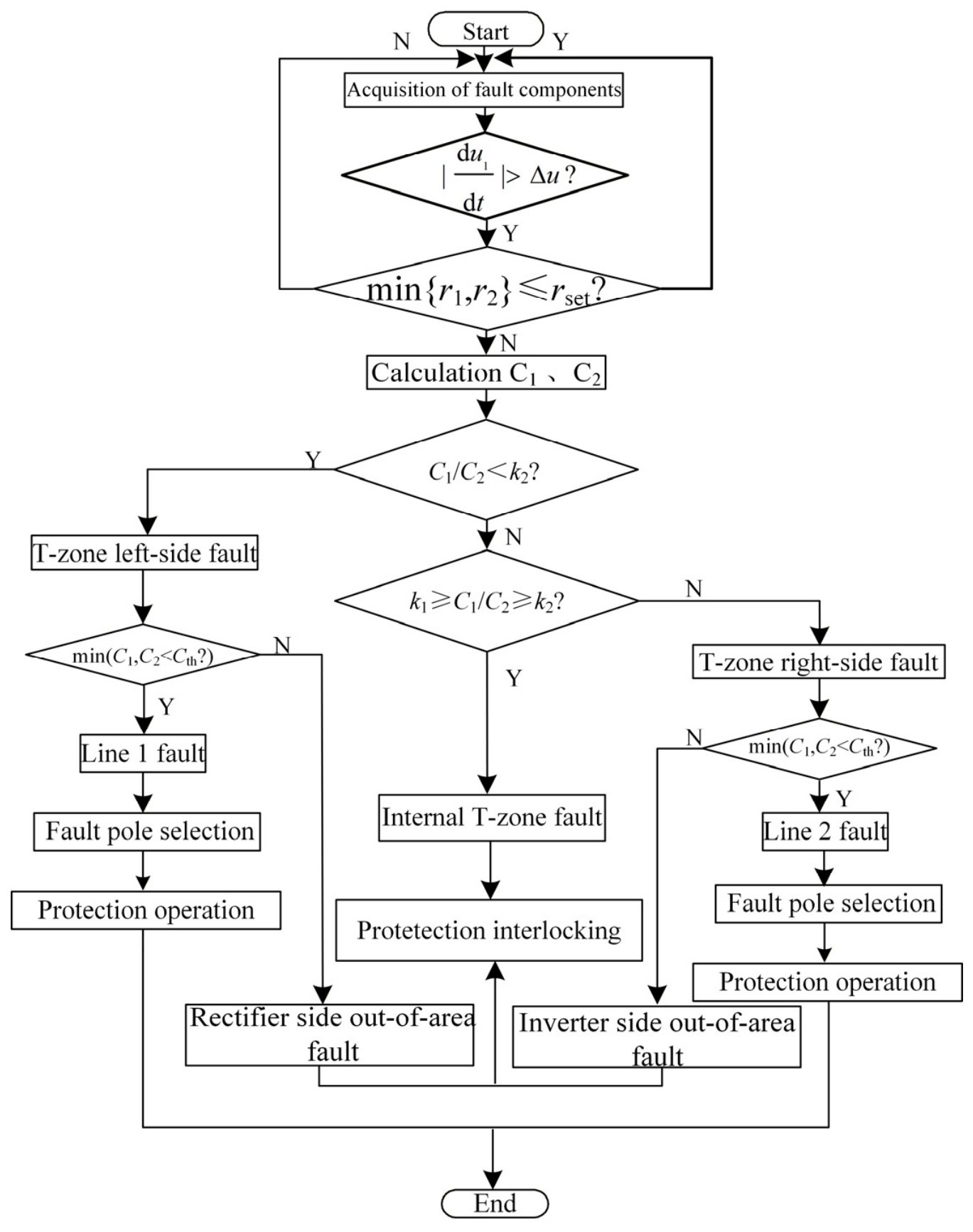
Through the construction of the start-up criterion, fault area discrimination criterion, pole selection criterion, and lightning disturbance identification criterion, a DC transmission line protection scheme based on the covariance values of the line-mode backward TWs is proposed, as illustrated in Figure 11.

4. Simulation Verification

The simulation model of the multi-terminal flexible HVDC transmission system is illustrated in Figure 12. The system adopts a symmetrical bipolar configuration with a voltage level of ±500 kV. Both the sending and receiving ends are constructed by connecting two 250 kV high- and low-voltage groups in series. Among them, MMC 1 operates as the sending-end rectifier station with a rated capacity of 400 MW, while MMC 2 and MMC 3 jointly constitute the receiving-end inverter stations, with rated capacities of 500 MW and 900 MW, respectively. The bridge-arm inductance is 30 mH, the equivalent capacitance of each submodule is 15 mF, the number of submodules per bridge arm is 200, and the current-limiting reactor is 20 mH. The DC transmission lines adopt frequency-dependent line models, with a total length of 500 km, consisting of Line 1 with a length of 300 km and Line 2 with a length of 200 km. The conductor height above ground is 34.5 m, the split-conductor spacing is 0.45 m, the effective distance between the positive and negative pole conductors is 18.25 m, and the vertical distance between the ground wires and the transmission conductors is 16.5 m. To evaluate the performance of the proposed protection scheme, metallic grounding faults are applied to both the positive and negative poles of the multi-terminal flexible HVDC system.

As shown in Figure 12, the fault locations include internal faults on Line 1 (f₁ and f₅), internal faults on Line 2 (f₃ and f₇), external faults on the rectifier side (f₂ and f₆), external faults on the inverter side (f₄ and f₈), and internal faults in the T-zone (f₉ and f₁₀).

4.1. Simulation Verification of the Protection Principle

Currently, the sampling frequency primarily utilized in DC transmission line protection ranges from 10 to 100 kHz. In this study, a sampling frequency of 50 kHz is adopted for fault simulation. Fault injection points are transiently configured at external locations, within the internal T-zone, and along Line 1 and Line 2, respectively. A post-fault data window of 0.5 ms is extracted for subsequent simulation calculations.

(1)

Fault on the Left Side of the T-zone

When a single-pole grounding fault occurs on the left side of the T-zone (at $f_1$ along $\mathrm{Line} 1$), the transient variations in the line-mode backward-traveling waves respectively measured by the protection devices on both sides of the T-zone, are illustrated in Figure 13.

As can be seen from Figure 13, selecting the 0.5 ms fault data after the occurrence of the fault on the left side of the $\mathrm{T}\text{-}\mathrm{zone}$, the line-mode backward TW detected by the left-side protection device of the $\mathrm{T}\text{-}\mathrm{zone}$ exhibits a declining trend, whereas that detected by the right-side protection device presents an initially declining and subsequently rising trend.

(2)

Faults on the right side of the $\mathrm{T}\text{-}\mathrm{zone}$

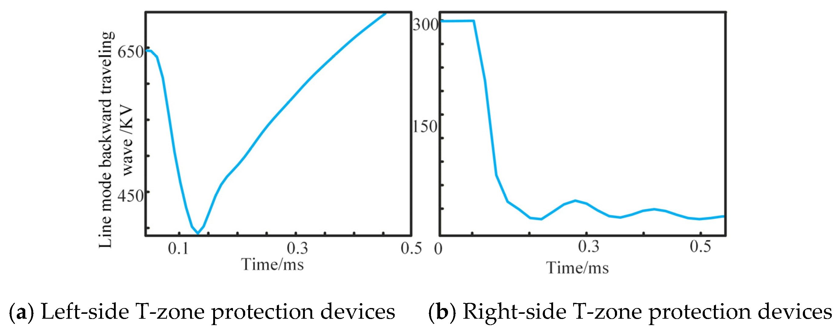
When a single-pole grounding fault occurs on the right side of the $\mathrm{T}\text{-}\mathrm{zone}$ (at $f_3$ along $\mathrm{Line} 2$), the variations in the backward TWs detected by the protection devices on both sides of the $\mathrm{T}\text{-}\mathrm{zone}$ are illustrated in Figure 14.

As can be observed from Figure 14, selecting the 0.5 ms fault data after the occurrence of the fault on the right side of the $\mathrm{T}\text{-}\mathrm{zone}$, the line-mode backward TW detected by the left-side protection device of the $\mathrm{T}\text{-}\mathrm{zone}$ exhibits a trend of initially declining and subsequently rising, whereas that detected by the right-side protection device presents a declining trend.

(3)

Internal T-zone Fault

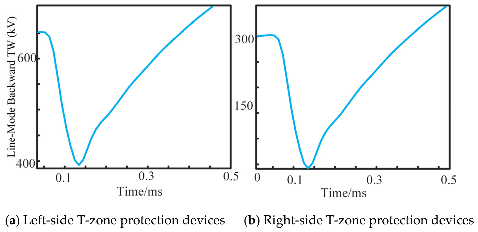
When a single-pole grounding fault occurs inside the $\mathrm{T}\text{-}\mathrm{zone}$ ($f_9$), Figure 15 illustrates the variations in the backward TWs detected by the protection devices installed on both sides of the $\mathrm{T}\text{-}\mathrm{zone}$.

As can be observed from Figure 15, when an internal fault occurs inside the $\mathrm{T}\text{-}\mathrm{zone}$, the line-mode backward TW detected by the left-side protection device of the $\mathrm{T}\text{-}\mathrm{zone}$ exhibits a trend of initially declining and subsequently rising, and similarly, the line-mode backward TW detected by the right-side protection device also presents an initially declining and subsequently rising trend.

(4)

External Faults Outside $\mathrm{MMC} 1$

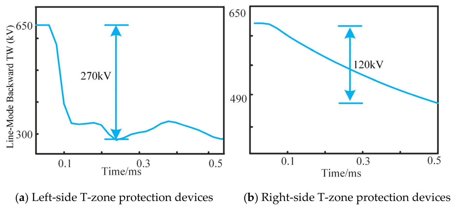
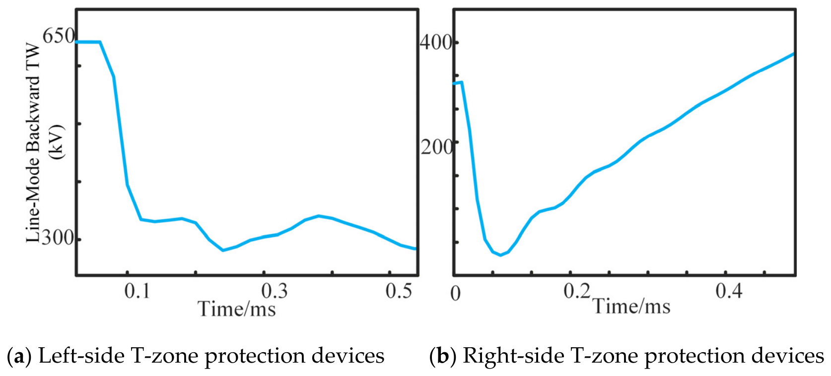
When a single-pole grounding fault occurs at the rectifier-side external fault location $f_2$ and the internal fault location $f_1$ along $\mathrm{Line} 1$, selecting the 0.5 ms fault data after the fault inception, the waveforms of the line-mode backward TW passing through the left-side protection device of the $\mathrm{T}\text{-}\mathrm{zone}$ are illustrated in Figure 16.

As can be seen from Figure 16a, when an internal fault occurs along $\mathrm{Line} 1$, the line-mode backward TW voltage detected by the left-side protection device of the $\mathrm{T}\text{-}\mathrm{zone}$ drops rapidly, with a voltage variation of approximately 270 kV. In contrast, when an external fault occurs outside $\mathrm{MMC} 1$, as illustrated in Figure 16b, the initial fault TW must propagate through the DCR before reaching the protection device. Due to the attenuation effect of the DCR, the declining trend of its wavefront is significantly mitigated, and the voltage variation is approximately 120 kV.

(5)

External Faults Outside $\mathrm{MMC} 3$

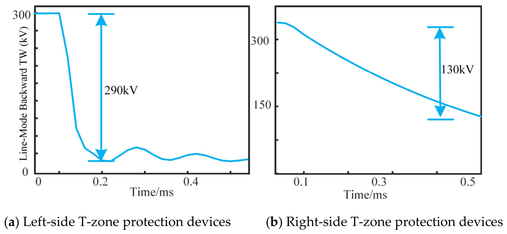
When a single-pole grounding fault occurs at the inverter-side external fault location $f_4$ and the internal fault location $f_3$ along $\mathrm{Line} 2$, selecting the 0.5 ms fault data after the fault inception, the voltage waveforms of the line-mode backward TW passing through the right-side protection device of the $\mathrm{T}\text{-}\mathrm{zone}$ are illustrated in Figure 17.

As illustrated in Figure 17, the voltage waveforms under faults internal and external to $\mathrm{MMC} 3$ also exhibit distinct discrepancies. Under an internal fault along $\mathrm{Line} 2$, the voltage drop detected by the right-side protection device of the $\mathrm{T}\text{-}\mathrm{zone}$ is approximately 290 kV. Conversely, under an external fault outside $\mathrm{MMC} 3$, affected by the attenuation effect of the DCR, the amplitude of the voltage drop decreases to approximately 130 kV, which is analogous to the scenario of the external fault outside $\mathrm{MMC} 1$.

To verify the reliability of the proposed scheme under different fault locations, simulation verifications are conducted for all the fault positions illustrated in Figure 12. The detailed results are summarized in

Table 1. Simulation Results of Positive-Pole Metallic Grounding Faults Under Different Fault Distances.

Fault Location		C1	C2	M	min(C1,C2)	K	Fault Direction
External to $\mathrm{MMC} 1$ f2		0.0332	0.0611	0.5433	0.0332	0.5066	Left side of the T-zone
Line 1 f1	0 km	−0.0151	0.0482	0.3132	−0.0151	0.2634	Left side of the T-zone
	20 km	−0.0266	0.0413	0.6440	−0.0266	0.2785	Left side of the T-zone
	50 km	−0.0075	0.0579	0.1295	−0.0075	0.3021	Left side of the T-zone
	90 km	0.0099	0.0653	0.1516	0.0099	0.3859	Left side of the T-zone
	100 km	0.0132	0.0652	0.2024	0.0132	0.4399	Left side of the T-zone
	120 km	0.0159	0.0742	0.2143	0.0159	0.4403	Left side of the T-zone
	140 km	0.0233	0.0752	0.3098	0.0233	0.4501	Left side of the T-zone
	160 km	0.0165	0.0763	0.2162	0.0165	0.4651	Left side of the T-zone
	180 km	0.0186	0.0797	0.2334	0.0186	0.4391	Left side of the T-zone
	200 km	0.0172	0.0789	0.2180	0.0172	0.4552	Left side of the T-zone
	240 km	0.0245	0.0810	0.3025	0.0245	0.3712	Left side of the T-zone
	260 km	0.0198	0.0796	0.2487	0.0198	0.3018	Left side of the T-zone
	280 km	0.0211	0.0776	0.2719	0.0211	0.4162	Left side of the T-zone
	300 km	0.0278	0.0781	0.3560	0.0278	0.2675	Left side of the T-zone
External to $\mathrm{MMC} 3$ f4		0.0500	0.0291	1.7182	0.0291	0.6652	Left side of the T-zone
Line 2 f3	0 km	0.0531	−0.0006	88.5000	−0.0006	0.1359	Right side of the T-zone
	30 km	0.0543	0.0021	25.85	0.0021	0.1721	Right side of the T-zone
	60 km	0.0622	0.0015	41.4667	0.0015	0.2029	Right side of the T-zone
	80 km	0.0698	0.0020	34.9000	0.0020	0.3041	Right side of the T-zone
	120 km	0.0616	0.0201	3.0640	0.0201	0.4623	Right side of the T-zone
	150 km	0.0632	0.0213	2.9671	0.0213	0.6174	Right side of the T-zone
	180 km	0.0661	0.0224	2.7500	0.0224	0.6372	Right side of the T-zone
	200 km	0.0634	0.0233	2.8430	0.0233	0.4434	Right side of the T-zone
f9 T-zone		0.0735	0.0723	1.0165	0.0723	0.5361	Inside the T-zone

and

Table 2. Simulation Results of Negative-Pole Metallic Grounding Faults Under Different Fault Distances.

Fault Location		C1	C2	M	min(C1,C2)	K	Fault Direction
External to $\mathrm{MMC} 1$ f6		0.0442	0.0603	0.733	0.0442	4.8352	Left side of the T-zone
Line 1 f5	0 km	−0.0023	0.0514	0.0447	−0.0023	5.5627	Left side of the T-zone
	20 km	−0.0116	0.0581	0.1996	−0.0116	5.5938	Left side of the T-zone
	50 km	0.0023	0.6014	0.0038	0.0023	6.0176	Left side of the T-zone
	90 km	0.0105	0.5922	0.0177	0.0105	6.3424	Left side of the T-zone
	100 km	0.0199	0.6634	0.0300	0.0199	6.5756	Left side of the T-zone
	120 km	0.0201	0.7843	0.0256	0.0201	6.3439	Left side of the T-zone
	140 km	0.0241	0.7645	0.3152	0.0241	5.9661	Left side of the T-zone
	160 km	0.0189	0.0718	0.2632	0.0189	6.0211	Left side of the T-zone
	180 km	0.0156	0.0723	0.2157	0.0156	5.5820	Left side of the T-zone
	200 km	0.0133	0.0684	0.1944	0.0133	5.2191	Left side of the T-zone
	240 km	0.0219	0.0885	0.2474	0.0219	5.1962	Left side of the T-zone
	260 km	0.0228	0.0752	0.4130	0.0228	4.5642	Left side of the T-zone
	280 km	0.0213	0.0771	0.2762	0.0213	4.4461	Left side of the T-zone
	300 km	0.0291	0.0756	0.3849	0.0291	4.3324	Left side of the T-zone
External to $\mathrm{MMC} 3$ f8		0.0512	0.0311	1.6463	0.0311	4.3021	Left side of the T-zone
Line 1 f7	0 km	0.0582	−0.0105	5.5428	−0.0105	5.1362	Right side of the T-zone
	30 km	0.0506	−0.0022	23.0000	−0.0022	5.7721	Right side of the T-zone
	60 km	0.0688	0.0141	4.8794	0.0141	5.7921	Right side of the T-zone
	80 km	0.0733	0.0182	4.0274	0.0182	5.5509	Right side of the T-zone
	120 km	0.0692	0.0287	2.4111	0.0287	5.4522	Right side of the T-zone
	150 km	0.0643	0.0299	2.1505	0.0299	6.0065	Right side of the T-zone
	180 km	0.0703	0.0251	2.8008	0.0251	4.3342	Right side of the T-zone
	200 km	0.0629	0.0206	3.0533	0.0206	4.3341	Right side of the T-zone
f10 T-zone		0.0721	0.0733	0.9836	0.0721	5.8129	Inside the T-zone

.

Taking the positive-pole line grounding faults along $\mathrm{Line} 1$ as an example for analysis, as the fault distance varies, the criterion value $M$ constantly remains below the setting threshold of 0.95, thereby being correctly identified as faults on the left side of the $\mathrm{T}\text{-}\mathrm{zone}$. Concurrently, since the minimum value of the covariance, denoted as $\min \left(C_1,C_2\right)$, is lower than the threshold of 0.04, it can be accurately classified as transmission line faults. Furthermore, within the pole selection criterion, the value of $K$ is consistently less than $1/1.212$, which guarantees the correct identification of positive-pole line faults. In summary, the comprehensive analysis of the data compiled in Table 1 and Table 2 demonstrates that the proposed protection scheme is entirely effective and reliable across all simulated fault locations within the model.

4.2. Transition Resistance and Noise Interference

To verify the effectiveness of the proposed protection scheme under different transition resistances, grounding faults via 150 Ω and 300 Ω transition resistances are set along the positive-pole line, respectively. The corresponding simulation results are summarized in

Table 3. Simulation Results Under Different Transition Resistances.

Fault Location	Transition Resistance (Ω)	C1	C2	M	min(C1,C2)	K	Fault Direction
External to $\mathrm{MMC} 1$ f2	150	0.0297	0.0621	0.5442	0.0338	0.5623	Left side of the T-zone
	300	0.0334	0.0618	0.5404	0.0334	0.5794	Left side of the T-zone
Line 1 f1 140 km	150	0.0254	0.0718	0.3537	0.0254	0.4927	Left side of the T-zone
	300	0.0299	0.0685	0.4365	0.0299	0.5113	Left side of the T-zone
External to $\mathrm{MMC} 1$ f4	150	0.0516	0.0224	2.3035	0.0224	0.6883	Right side of the T-zone
	300	0.0501	0.0277	1.8086	0.0277	0.6243	Right side of the T-zone
Line 2 f3 120 km	150	0.0698	0.0193	3.6165	0.0193	0.5901	Right side of the T-zone
	300	0.0701	0.0231	3.0346	0.0231	0.6001	Right side of the T-zone
f9 T-zone	150	0.0711	0.0699	1.0171	0.0699	0.5370	Inside the T-zone
	300	0.0692	0.0696	0.9942	0.0692	0.5466	Inside the T-zone

.

As can be observed from Table 3, with the increase in transition resistance, the fault current decreases, and the amplitude of the initial line-mode backward TW diminishes accordingly. Consequently, the original covariance is susceptible to variations in amplitude. In this paper, the normalized covariance is adopted as the criterion, and the waveform is normalized prior to the covariance calculation. This approach effectively eliminates the adverse effects brought by amplitude discrepancies, ensuring that the criterion predominantly reflects the overall variation trend of the waveform rather than its absolute magnitude. Therefore, the covariance values undergo only minor fluctuations as the transition resistance increases and can still fully satisfy the proposed fault discrimination criterion, demonstrating that the proposed protection scheme possesses high robustness against transition resistance.

To verify whether noise interference compromises the reliability of the protection scheme, several typical fault locations along the positive-pole line are selected. Gaussian white noise with signal-to-noise ratios (SNRs) of 20 dB, 30 dB, and 40 dB is respectively added to the detected line-mode backward TWs. The corresponding simulation results are summarized in

Table 4. Simulation Results Under Different Noise Interferences.

Fault Location	Noise (db)	C1	C2	M	min(C1,C2)	K	Fault Direction
External to $\mathrm{MMC} 1$ f2	20	0.0330	0.0613	0.5384	0.0330	0.5105	Left side of the T-zone
	30	0.0335	0.0609	0.5500	0.0335	0.5082	Left side of the T-zone
	40	0.0299	0.0618	0.4838	0.0299	0.5114	Left side of the T-zone
Line 1 f1 140 km	20	0.0218	0.0742	0.2938	0.0218	0.4881	Left side of the T-zone
	30	0.0203	0.0715	0.2979	0.0203	0.5202	Left side of the T-zone
	40	0.0220	0.0731	0.3009	0.0220	0.4879	Left side of the T-zone
External to $\mathrm{MMC} 3$ f4	20	0.0488	0.0288	1.6944	0.0288	0.6650	Right side of the T-zone
	30	0.0482	0.0281	1.7153	0.0281	0.6642	Right side of the T-zone
	40	0.0475	0.0273	1.7399	0.0273	0.6648	Right side of the T-zone
Line 2 f3 120 km	20	0.0612	0.0199	3.0753	0.0199	0.4829	Right side of the T-zone
	30	0.0615	0.0203	3.0295	0.0203	0.5013	Right side of the T-zone
	40	0.0600	0.0201	2.9850	0.0201	0.5001	Right side of the T-zone
f9 $\mathrm{T}\text{-}\mathrm{zone}$	20	0.0730	0.0729	1.0013	0.0729	0.5410	Inside the T-zone
	30	0.0733	0.0734	0.9886	0.0733	0.5386	Inside the T-zone
	40	0.0728	0.0729	0.9986	0.0728	0.5620	Inside the T-zone

.

As shown in Table 4, the normalized covariance values exhibit only slight fluctuations as the noise level increases and always remain within the corresponding decision thresholds. This is because the proposed protection scheme determines the fault region according to the overall variation trend of the line-mode backward traveling wave rather than the wavefront or local transient features. Although noise introduces minor local waveform disturbances, it does not alter the overall waveform trend. Consequently, the normalized covariance is only slightly affected, and the proposed protection criterion remains reliable.

4.3. Lightning Disturbance

To verify the effectiveness of the proposed lightning disturbance identification criterion, several typical lightning disturbances and short-circuit fault conditions are selected for simulation verification. Taking positive-pole faults as an example, short-circuit faults are configured with various scenarios, including 0 Ω metallic grounding and 300 Ω high-resistance grounding, at different locations such as $\mathrm{Line} 1$, outside $\mathrm{MMC} 1$, and inside the $\mathrm{T}\text{-}\mathrm{zone}$. The amplitude of the lightning current is set to 10 kA, and the setting threshold for lightning disturbances, denoted as $r_{\mathrm{set}}$, is selected as 0.5. The corresponding simulation results are summarized in

Table 5. Simulation Results of Lightning Interference Identification Criteria.

Fault/Lightning Disturbance	$\mathbf{min}\left\{{\mathit{r}}_1,{\mathit{r}}_2\right\}$	Fault Identification Result
Lightning strike (8/20 μs)	0.12	Lightning strike
Lightning strike (1.2/50 μs)	0.17	Lightning strike
Lightning strike (10/350 μs)	0.23	Lightning strike
Line 1 internal fault f1 = 50 km, Rf = 0 Ω	0.75	Fault
Line 1 internal fault f1 = 50 km, Rf = 300 Ω	0.72	Fault
Line 1 internal fault f1 = 180 km, Rf = 0 Ω	0.74	Fault
Line 1 internal fault f1 = 180 km, Rf = 300 Ω	0.68	Fault
Line 1 internal fault f1 = 320 km, Rf = 0 Ω	0.97	Fault
Line 1 internal fault f1 = 320 km, Rf = 300 Ω	0.93	Fault
Internal T-zone fault f10, Rf= 0 Ω	0.79	Fault
Internal T-zone fault f10, Rf = 300 Ω	0.73	Fault

.

As can be observed from Table 5, when lightning disturbances are applied, the calculated criterion values are all less than the setting threshold, which are correctly identified as “lightning disturbances.” Conversely, under all short-circuit fault conditions, regardless of variations in the fault location or transition resistance, the calculated criterion values consistently exceed the setting threshold of 0.5, and all are correctly identified as “faults.” Therefore, it can be concluded that this criterion can clearly quantify the significant discrepancy in waveform attenuation rates between lightning disturbances and short-circuit faults, effectively distinguishing between these two different types of disturbances. This fully validates the reliability and accuracy of the proposed criterion.

4.4. Compared with Existing Protection Schemes

To validate the superiority of the proposed protection scheme, a quantitative numerical comparison is conducted between the proposed method and three existing typical protection schemes. The benchmark methods include: the DC reactor voltage rate of change method proposed in [23], the wavelet transform-based high-frequency feature extraction method proposed in [24], and the artificial intelligence (AI)-based (CNN-Transformer) fault identification method proposed in [25]. The comparison results are summarized in

Table 6. Performance comparison between the proposed method and existing DC fault protection schemes.

Performance Metric	Ref. [23]	Ref. [24]	Ref. [25]	Proposed Method
System type	Multi-terminal VSC-HVDC	VSC-HVDC transmission system	Meshed multi-terminal MMC-HVDC	Three-terminal MMC-based flexible HVDC system with T-connection
Principle	Deep learning for fault temporal feature learning	Boundary reactor high-frequency attenuation	DCR voltage rate (equivalent to 2nd current derivative)	Waveform trend similarity of line-mode backward TWs quantified by normalized covariance
Methodology	CNN-Transformer hybrid model inference	First-scale SWT feature extraction	Dual-threshold time interval + polarity discrimination	Normalized covariance
Sampling Frequency	50~100 kHz	100 kHz~1 MHz	13.5 kHz	50 kHz
Operating Time	1.4 ms	1~3 ms	4.89 ms	0.5 ms
Transition Resistance Tolerance	100 Ω	1000 Ω	100 Ω	300 Ω
Noise Robustness	No quantitative noise test	66.02 dB	20 dB	40 dB
Communication Requirement	None	None	None	None
Computational Complexity	Low. Requires only time-domain voltage threshold comparison and differential calculations; simple logic, easy engineering implementation.	Moderate. Requires first-scale stationary wavelet filter operations.	High. Deep learning model inference requires considerable computing power; high training costs, relying on high-performance processors.	Low. Involves only waveform normalization and covariance calculations.

.

5. Conclusions

A single-ended directional protection scheme based on the covariance of line-mode backward traveling waves is proposed for multi-terminal flexible DC transmission lines. By utilizing the protection devices installed on both sides of the $\mathrm{T}\text{-}\mathrm{zone}$, the fault area can be successfully identified by calculating the covariance between the line-mode backward TW and the reference waveform. The main conclusions are summarized as follows:

(1)

A single-ended traveling-wave protection scheme applicable to the T-connection area of MMC-based multi-terminal flexible DC transmission systems is proposed. The protection devices are deployed inside the same converter station on both sides of the $\mathrm{T}\text{-}\mathrm{zone}$. Fault discrimination can be accomplished by relying solely on locally collected electrical quantities without the need for long-distance communication or time synchronization, thereby eliminating the adverse impacts of communication latencies and synchronization errors on protection performance.

(2)

A normalized covariance criterion based on the overall variation trend of the line-mode backward TW is constructed. Distinct from traditional protection methods that rely on frequency-domain features such as high-frequency energy or wavelet coefficients, the proposed criterion circumvents the extraction of specific high- or low-frequency components and directly quantifies the overall similarity of the waveforms. The normalization pre-processing effectively mitigates the impacts of waveform amplitude variations on the criterion, thereby reducing the sensitivity of the algorithm to fluctuations in sampling frequency and transition resistance.

(3)

Under the built PSCAD simulation model and test scenarios in this study, the proposed protection scheme can complete fault discrimination within a data window of only 0.5 ms after the protection is initiated. The protection remains entirely valid even when the sampling frequency drops to 50 kHz. Furthermore, the scheme can reliably identify faults under the conditions of a 300 Ω transition resistance and 40 dB Gaussian white noise, demonstrating that the proposed method possesses excellent operating speed, high robustness against transition resistance, and strong immunity to noise interference.

(4)

It should be noted that the proposed scheme is currently validated entirely via PSCAD simulations, without fully accounting for practical hardware delays and sampling jitter. Therefore, the lack of Hardware-in-the-Loop (HIL) or real-time simulation (e.g., RTDS) testing represents a limitation of this work. As a key direction for future research, an RTDS-based HIL experimental platform will be constructed to further evaluate the scheme’s reliability and engineering feasibility in real hardware environments.

References

1. Ma, J.; Hong, L.; Zhou, X.; Deng, L.; Peng, H.; Zhu, R. Transient Response Analysis and System Fault Ride-Through Capability Optimization of HVDC Based on Hybrid Commutated Converter. IEEE Trans. Power Deliv. 2026, 41, 901–913. [Google Scholar] [CrossRef] [Scilit]
2. Guo, C.; Liu, Y.; Zhao, C.; Wei, X.; Xu, W. Power component fault detection method and improved current order limiter control for commutation failure mitigation in HVDC. IEEE Trans. Power Deliv. 2015, 30, 1585–1593. [Google Scholar] [CrossRef] [Scilit]
3. Xue, Y.; Zhang, X.P.; Yang, C. AC filter less flexible LCC HVDC with reduced voltage rating of controllable capacitors. IEEE Trans. Power Syst. 2018, 33, 5507–5518. [Google Scholar] [CrossRef] [Scilit]
4. Guo, Z.L.; Hao, L.L.; He, J.H.; Chen, Z.G.; Wang, X.G. Complete protection strategy for loss of excitation in large-scale synchronous condensers applied to UHVDC transmission. CSEE J. Power Energy Syst. 2025, 11, 919–930. [Google Scholar] [CrossRef] [Scilit]
5. Tang, Y.; Li, F.; Wang, Q.; Chen, B.; Jiang, Y.L.; Guo, X.J. Power stability analysis of UHVDC systems hierarchically connected to AC systems. Electr. Power Syst. Res. 2018, 163, 715–724. [Google Scholar] [CrossRef] [Scilit]
6. Cai, H.; Wang, G.; Xie, Z.; Huang, J.; Zhang, J.; Xu, Z. Analysis on the safety and stability of flexible direct-current transmission technology in multi-infeed-direct-current receiving-end transmission power systems. In Proceedings of the 16th IET International Conference on AC and DC Power Transmission (ACDC 2020), Online Conference; Institution of Engineering and Technology (IET): London, UK; Stevenage, UK, 2020; pp. 238–243. [Google Scholar]
7. Xing, C.; Liu, M.; He, X.; Xi, X. Research on flexible control technology of HVDC. In Proceedings of the 2019 IEEE 8th International Conference on Advanced Power System Automation and Protection (APAP), Xi’an, China, 21–24 October 2019; pp. 1186–1190. [Google Scholar]
8. Cai, H.; Wang, G.; Xie, Z.; Huang, J.; Zhang, J.; Xu, Z. Research on the application of flexible direct-current transmission technology in the system planning integrated with large scale of offshore wind farms. In Proceedings of the 16th IET International Conference on AC and DC Power Transmission (ACDC 2020), Online Conference; Institution of Engineering and Technology (IET): London, UK; Stevenage, UK, 2020; pp. 339–343. [Google Scholar]
9. Rao, H.; Zou, C.; Xu, S.; Cai, X.; Li, Y.; Zhao, X. The On-site Verification of Key Technologies for Kunbei-Liuzhou-Longmen Hybrid Multi-terminal Ultra HVDC Project. CSEE J. Power Energy Syst. 2022, 8, 1281–1289. [Google Scholar] [CrossRef] [Scilit]
10. Pragati, A.; Mishra, M.; Rout, P.K.; Gadanayak, D.A.; Hasan, S.; Prusty, B.R. A comprehensive survey of HVDC protection system: Fault analysis, methodology, issues, challenges, and future perspective. Energies 2023, 16, 4413. [Google Scholar] [CrossRef] [Scilit]
11. Xiao, H.; Li, Y.; Ren, S. Novel disturbance blocking criterion for reliable current differential protection of LCC-HVDC lines. IEEE Trans. Power Deliv. 2021, 36, 477–480. [Google Scholar] [CrossRef] [Scilit]
12. Han, K.; Chen, Y.; We, M.; Ma, R. A novel pilot protection scheme based on differential voltage for hybrid LCC/MMC HVDC transmission lines. IEEE Trans. Power Deliv. 2024, 39, 1816–1826. [Google Scholar] [CrossRef] [Scilit]
13. Tourn, D.H.; Florena, E.; Zamanillo, G.; Donolo, P.D.; Dissanayake, A.; Kulkarni, P.; Hartshorn, J.; Donolo, M. Signal processing for high impedance differential protection schemes. IEEE Trans. Ind. Appl. 2024, 60, 7702–7710. [Google Scholar] [CrossRef] [Scilit]
14. Li, C.; Go, A.M.; Zhao, C. A fast DC fault detection method Using DC reactor voltages in HVdc Grids. IEEE Trans. Power Deliv. 2018, 33, 2254–2264. [Google Scholar] [CrossRef] [Scilit]
15. Pérez-Molina, M.J.; Larruskain, D.M.; Eguía, P.; Santiago, V.V. Local derivative-based fault detection for HVDC grids. IEEE Trans. Ind. Appl. 2022, 58, 1521–1530. [Google Scholar] [CrossRef] [Scilit]
16. Geddada, N.; Yeap, Y.M.; Ukil, A. Experimental validation of fault identification in VSC-based DC grid system. IEEE Trans. Ind. Electron. 2018, 65, 4799–4809. [Google Scholar] [CrossRef] [Scilit]
17. Li, B.; Li, Y.; He, J.; Li, B.; Liu, S.; Liu, B.; Xu, L. An improved transient traveling-wave based direction criterion for multi-terminal Hvdc grid. IEEE Trans. Power Deliv. 2020, 35, 2517–2529. [Google Scholar] [CrossRef] [Scilit]
18. Mu, D.; Lin, S.; He, P.; Li, X. An Improved Method of Traveling Wave Protection for DC Lines Based on the Compensation of Line-Mode Fault Voltage. IEEE Trans. Power Deliv. 2023, 38, 1720–1730. [Google Scholar] [CrossRef] [Scilit]
19. Wu, J.; Li, H.; Wang, G.; Liang, Y. An Improved Traveling-Wave Protection Scheme for LCC-HVDC Transmission Lines. IEEE Trans. Power Deliv. 2017, 32, 106–116. [Google Scholar] [CrossRef] [Scilit]
20. Wang, Y.; Zhang, B.; Fan, X. The overhead transmission line protection scheme for the voltage-source converter-based HVDC grids. J. Eng. 2019, 2019, 674–679. [Google Scholar] [CrossRef] [Scilit]
21. Ha, H.X.; Yu, Y.; Yi, R.P.; Bo, Z.Q.; Chen, B. Novel scheme of travelling wave based differential protection for bipolar HVDC transmission lines. In Proceedings of the 2010 International Conference on Power System Technology, Hangzhou, China, 24–28 October 2010; pp. 1–6. [Google Scholar]
22. Xie, F.; Hao, Z.; Ye, D.; Zhang, B.; Liu, Z. A RFTR based lightning disturbance identification scheme for VSC-HVDC line protection. In Proceedings of the Tsinghua University-IET Electrical Engineering Academic Forum: Constructing Green and Sustainable Energy System (2021), Beijing, China, 15–16 May 2021; pp. 75–80. [Google Scholar]
23. Li, R.; Xu, L.; Yao, L. Dc fault detection and location in meshed multiterminal Hvdc systems based on Dc reactor voltage change rate. IEEE Trans. Power Deliv. 2017, 32, 1516–1526. [Google Scholar] [CrossRef] [Scilit]
24. Silva, D.M.; Costa, F.B.; Franca, R.L.S.; Junior, F.C.S. Wavelet-Based Detection of Transients Induced by DC Faults Using Boundary Protection Principle. In Proceedings of the 2018 IEEE Power & Energy Society General Meeting (PESGM), Portland, OR, USA, 5–10 August 2018; pp. 1–5. [Google Scholar]
25. Mishra, M.; Singh, J.G. Fault Detection and Localization in an MT-VSC-HVDC Network via a Hybrid CNN-Transformer Model With a Multi-Head Attention Mechanism. IEEE Access 2025, 13, 26365–26383. [Google Scholar] [CrossRef] [Scilit]
Figure 1. Topology Diagram of a Multi-Terminal Flexible HVDC Transmission System.
Energies 19 04400 g001
Figure 2. Schematic Diagram of Traveling-Wave Reflection and Transmission for a Fault on Line 1 on the Left Side of the T-zone.
Energies 19 04400 g002
Figure 3. The line-mode backward traveling wave u b 11 L after the fault.
Energies 19 04400 g003
Figure 4. Schematic diagram for a Fault on Line 1 on the Left Side of the T-zone.
Energies 19 04400 g004
Figure 5. Simulation and theoretical waveforms of u b 21 L .
Energies 19 04400 g005
Figure 6. Schematic diagram of fault TW reflection and transmission under a fault on the right side of the T-zone.
Energies 19 04400 g006
Figure 7. Schematic diagram for a Fault on Line 2 on the Right Side of the T-zone.
Energies 19 04400 g007
Figure 8. Diagram of fault TW reflection in T-zone.
Energies 19 04400 g008
Figure 9. Equivalent Circuit Diagram for a Fault in a T-zone.
Energies 19 04400 g009
Figure 10. Fault equivalent circuit for an external fault outside MMC   1 .
Energies 19 04400 g010
Figure 11. Fault discrimination flowchart for multi-terminal MMC-HVDC transmission lines based on the normalized covariance of line-mode backward TWs.
Energies 19 04400 g011
Figure 12. Simulation Model of a Three-Terminal Flexible HVDC System.
Energies 19 04400 g012
Figure 13. Line-mode backward TWs detected by protection devices on both sides under a fault on the left side of the T - zone .
Energies 19 04400 g013
Figure 14. Line-mode backward TWs detected by protection devices on both sides under a fault on the right side of the T - zone .
Energies 19 04400 g014
Figure 15. Line-mode backward TWs detected by protection devices on both sides under an internal fault inside the T - zone .
Energies 19 04400 g015
Figure 16. Comparison of line-mode backward TWs detected by the left-side protection device of the T - zone under faults internal and external to MMC   1 .
Energies 19 04400 g016
Figure 17. Line-mode backward TWs detected by the right-side protection devices under internal and external faults associated with MMC 3.
Energies 19 04400 g017