Customer–Meter Box Relationship Identification Based on Load Switching Dynamic Response

Abstract

Within the same low-voltage distribution network (LVDN), the short electrical distances between customers lead to highly similar steady-state voltage curves. This reduces the discriminative capability of traditional similarity metrics and limits the accuracy of customer–meter box relationship identification. To address this problem, this paper proposes a two-stage framework for identifying customer–meter box relationships based on dynamic responses to load switching. In the first stage, the consistency of the dynamic voltage responses of same-phase customers within the same meter box is used to calculate the similarity between customers voltage event sequences. The customers are then divided into single-phase clusters by phase. In the second stage, using the current events generated by load switching as the driving quantity and the cross-phase voltage events as the response quantity, a cross-phase cluster matching model is constructed. Combined with a voting mechanism and an optimized allocation strategy, this approach enables accurate matching of single-phase clusters across different phases and complete reconstruction of the meter box topology. A case study using high-frequency measurement data from an actual LVDN in Nanjing shows that the proposed method achieves an identification accuracy of 100%, demonstrating its effectiveness and superiority in identifying the meter boxes assignments of customers that are electrically close to one another.

1. Introduction

As the “last mile” connecting the power system to end customers, the operational status of low-voltage distribution networks (LVDNs) directly affects the quality and safety of power supply services. Therefore, accurate topological connections are essential for the operation and maintenance of LVDNs [1,2,3,4]. In recent years, with the large-scale integration of distributed renewable energy sources and the rapid growth of emerging loads such as electric vehicles and smart homes, the operating environment of LVDNs has become increasingly complex [5,6]. Meanwhile, due to factors such as the large scale of equipment, the limited level of intelligence, and inconsistent communication protocols, the actual topology of LVDNs often differs from the records. And this significantly increases the difficulty of operational monitoring and maintenance management [7]. In addition, during the long-term operation of LVDNs, the connection relationships among transformers, lines, meter boxes and customers are frequently changed, and some line routes are concealed. These uncertainties further increase the inaccuracy of topology information [8].

Many existing studies on LVDNs have focused on identifying customer–transformer and customer–phase relationships, while research on customer–meter box relationship identification remains insufficient. Most existing studies use smart meter measurements and employ clustering, unsupervised learning, joint optimization, and graph neural network methods to identify customer–transformer relationship [9,10,11,12,13], while correlation and clustering have been employed to identify customer–phase relationship [14,15,16,17]. In [18], a data segmentation method was proposed to jointly identify customer–transformer and customer–phase relationships. The meter box is an important management unit for metering assets in LVDNs. The customer–meter box relationship denotes the physical association between a customer"s smart meter and the shared meter box in which it is installed, not the billing customer–meter relationship. In practice, new customer connections and capacity expansions, network upgrades, and emergency repairs frequently change customer–meter box connections, making manual verification methods inadequate to address the dual challenges of the scale and dynamic evolution of LVDNs [19,20].

At present, studies on the identification of customer–meter box relationships in LVDNs mainly use data-driven methods. These methods identify the customer–meter box relationships by extracting the characteristics of the collected steady-state voltage curves data. Reference [21] clustered customers based on the correlations among the steady-state voltage curves measured by their electricity meters. A quadratic programming model was then developed to identify customer–meter box relationship identification. Lian et al. [22] proposed a customer–meter box relationship identification method based on t-distributed stochastic neighbor embedding (t-SNE) for dimensionality reduction and balanced iterative reducing and clustering using hierarchies (BIRCH). First, t-SNE was used to reduce the dimensionality of large amounts of high-dimensional voltage data collected by the smart electricity meters and extracted the main features. BIRCH was employed to cluster the data after dimensionality reduction, achieving the identification of the phase and meter box affiliation for single-phase customers. With the customer phases known, Luo et al. [23] used voltage curves to cluster the customers of each phase at the distribution branch-box level. Neighborhood relationships, such as building and unit information in customer addresses, were then converted into constraints. An improved constrained K-medoids algorithm was further used to identify the meter box associated with each customer. Based on voltage correlation, Xu et al. [24] used extreme point detection and a constrained hidden Markov model to dynamically segment the voltage time series. Phase and meter box identification was then performed for single-phase customers according to the Pearson correlation between the segmented sequences.

Overall, at present, relatively few studies have investigated the identification of customer–meter box relationships. The data-driven methods rely on extracting discriminative features from the voltage curves of customers connected to different meter boxes. However, adjacent meter boxes within the same LVDN are close in both physical and electrical distance. Their supply paths largely overlap, and the impedance differences between their non-common line sections are small. Consequently, the voltage curves of customers connected to neighboring meter boxes are highly similar. Therefore, existing clustering methods based on the differences in steady-state voltage curves have certain limitations in identifying the relationships between customers and meter boxes. Moreover, most of these methods can only identify the phase and meter box to which single-phase customers belong within the same LVDN but cannot resolve the meter box assignment issue for complete three-phase customers. Considering the inherent limitations of the above methods, this paper proposes a customer–meter box relationship identification method based on dynamic responses to load switching.

This method systematically analyzes the load fluctuation characteristics caused by differences in electrical distance among different meter box customers, as well as the cross-phase coupling mechanism caused by neutral-conductor impedance among customers within the same meter box. By analyzing high-frequency voltage and current data, it captures load switching events and quantifies the resulting dynamic response characteristics. This overcomes the limitation of conventional methods that use steady-state voltage curves features to identify the meter box associations of electrically close customers. However, increasing rooftop PV penetration may introduce reverse power flows and alter local voltage–current responses in LVDNs. Smart-inverter control, switching dynamics, and converter-induced harmonic distortion may further mask or distort the transient voltage signatures associated with load-switching events [25,26,27], introducing additional uncertainties into voltage-response-based topology identification. The main contributions of this paper are as follows: (1) models of cross-phase coupling within meter boxes and dynamic load responses between meter boxes in load switching events are established; (2) a two-stage identification strategy is proposed. First, same-phase customers are clustered based on the high consistency of the dynamic responses of customers within the same meter box. Then, event association matching is performed using the cross-phase coupling effect to establish complete customer–meter box topology.

2. Analysis of Dynamic Response Characteristics of Load Switching

The operating state of an LVDN is jointly influenced by its topology and the electricity consumption behavior of customers. During steady-state operation, the voltage differences among various nodes are relatively small. However, load switching events, especially the switching on and off of high-power loads, cause observable voltage fluctuations within the same low-voltage distribution network, thereby providing an effective basis for identifying the network topology.

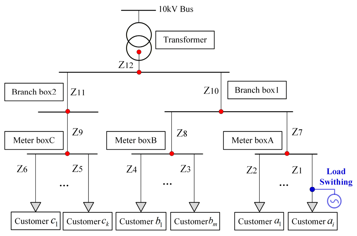
Figure 1 shows the topology of a three-phase four-wire LVDN, with phase A customers taken as an example. Electrical energy is transmitted from the secondary side of the transformer through the branch boxes to the meter boxes. The meters of same-phase customers within the same meter box are connected in parallel to the internal busbar, and each customer is assumed to be located at the position of the corresponding meter. Since the electrical distance between customers is extremely short, the contact impedance is only at the micro-ohm level, which can be neglected compared to the line impedance. When load switching occurs at a customer, the current disturbance produces complex voltage responses through the impedances of phase conductors and neutral conductors. This process not only causes highly synchronized voltage responses among same-phase customers within the same meter box but also affects customers of different phases through coupling via the neutral conductor and causes differences in voltage responses. This feature provides a theoretical basis for quantifying the effects of load switching events.

Suppose the event source customer $a_i$ belongs to Phase A; when a load switching event occurs, it causes a change in the operating current $\Delta {\dot{I}}_A$. Let the phase conductor impedances of phases A, B, C be $Z_A,Z_B,Z_C$ respectively and the neutral-conductor impedances be $Z_N$. The following assumptions are made: (1) The reference phase angles of phases A, B, and C are 0°, −120°, and 120° respectively [28]. (2) The internal impedances of the power source and the transformer are converted to obtain the equivalent source impedance $Z_S$ for each phase.

2.1. Customers on the Same Phase Within the Same Meter Box

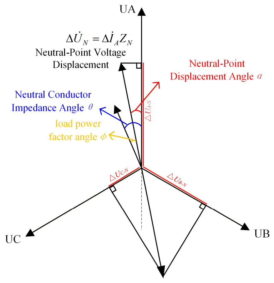
Figure 2 illustrates the principle of the dynamic response caused by load switching events in a three-phase, four-wire system. First, the switching event causes a change in the current of phase A, and it flows through the phase conductor impedance and the neutral-conductor impedance. According to Kirchhoff"s voltage law (KVL) and the node voltage method, the resulting voltage change $\Delta {\dot{U}}_A$ for a phase A customer within the same meter box can be expressed as

$$\Delta {\dot{U}}_A=-(\Delta {\dot{I}}_A{Z}_A+\Delta {\dot{I}}_A{Z}_S+\Delta {\dot{U}}_N)$$

(1)

where $\Delta {\dot{U}}_N$ represents the neutral-point voltage displacement caused by the change in the phase A current:

$$\Delta {\dot{U}}_N=\Delta {\dot{I}}_N{Z}_N=\Delta {\dot{I}}_A{Z}_N$$

(2)

By substituting Equation (2) into Equation (1), the total voltage change of the phase A customer can be decomposed into two components: the phase conductor voltage-drop component and the neutral-conductor component.

$$\Delta {\dot{U}}_A=-\Delta {\dot{I}}_A(Z_A+Z_S)+(-\Delta {\dot{I}}_A{Z}_N)$$

(3)

With the phase A voltage taken as the reference direction, the angle by which the load current lags the phase A voltage is defined as the load power factor angle ϕ. The projections of the two components onto the phase A reference direction are analyzed respectively.

(1)

Projection of the phase conductor voltage-drop component

Let the impedance angle of $Z_A+Z_S$ be ${\mathsf{\theta }}_{AS}$. Then the projection of the phase conductor voltage-drop component in the direction of phase A is

$$\Delta {\dot{U}}_{l-A}=-\Delta {\dot{I}}_A|Z_A+Z_S|\cos ({\mathsf{\theta }}_{AS}-\varphi )$$

(4)

In LVDNs, the impedances of the phase conductors are dominated by their resistive components. In this study, LVDN lines refer to the phase conductors extending from the transformer secondary through branch boxes to meter boxes. A review of the cable types commonly used for these lines shows that the impedance angle $Z_A$ is $3°–18°$. Although the equivalent source impedance $Z_S$ is mainly inductive, its magnitude is much smaller than $\left|Z_A\right|$ (approximately 1/3 to 1/5 of $\left|Z_A\right|$), and the typical range of the resultant impedance angle ${\mathsf{\theta }}_{AS}$ is $3°–25°$. The load power factor angle ϕ should account for common household loads, such as air conditioners and electric water heaters, whose power factors are generally 0.8–1, corresponding to the phase angle ϕ range of approximately $0°–30°$. Therefore, we can obtain $|{\mathsf{\theta }}_{AS}-\varphi |<<90°$ and $\cos ({\mathsf{\theta }}_{AS}-\varphi )>0$, that is, $\Delta {\dot{U}}_{l-A}<0$, manifests as a voltage drop.

(2)

Projection of the neutral-conductor component

Define the neutral-point displacement angle $\alpha$:

$$\alpha =\arctan ({\displaystyle \frac{X_N}{R_N}})+\varphi$$

(5)

where $X_N$ and $R_N$ represent the reactance and resistance of the corresponding neutral conductor respectively; then the component of the neutral-point voltage displacement in the phase A direction is

$$\Delta U_{N-A}=-|\Delta {\dot{U}}_N|\cos \alpha$$

(6)

In LVDNs, the resistance $R$ is usually greater than the reactance $X$; the value of $R:X$ is generally greater than 2, so the range of the $\arctan (X_N/R_N)$ component in $\alpha$ is $0°–30°$ [29]. The load power factor angle $\varphi$ ranges from $0°–30°$. Therefore, the range of $\alpha$ is approximately at $(-30°,30°)$, and we can obtain $\cos (\alpha )>0$. Thus, the projection $\Delta U_{N-A}<0$ of phase A reference direction shows a voltage drop.

Combining the above two components, the total voltage change measured by the phase A customers is

$$\Delta {\dot{U}}_A=\Delta {\dot{U}}_{l-A}+\Delta {\dot{U}}_{N-A}=-\Delta {\dot{I}}_A|Z_A+Z_S|\cos ({\mathsf{\theta }}_{AS}-\varphi )-|\Delta {\dot{U}}_N|\cos \alpha$$

(7)

Since both components are negative, phase A customers necessarily experience a voltage drop. The magnitude of the voltage drop mainly depends on the magnitudes of the phase conductor impedance $Z_A$, the neutral-conductor impedance $Z_N$, and equivalent source impedance $Z_S$. Under typical parameter conditions, the magnitude of the voltage drop increases as the above impedances increase.

2.2. Customers on Different Phases Within the Same Meter Box

Although customers on the non-event phases within the same meter box have no changes in their own currents ($\Delta {\dot{I}}_B=0,\Delta {\dot{I}}_C=0$), they are affected by the coupling effect of the phase A switching event through the shared neutral-conductor impedance $Z_N$. The voltage change component on the non-event phase affected by the neutral-point voltage displacement can be expressed as

$$\Delta U_{N-B}=-|\Delta {\dot{U}}_N|\cos (\alpha °+120°)$$

(8)

$$\Delta U_{N-C}=-|\Delta {\dot{U}}_N|\cos (\alpha °-120°)$$

(9)

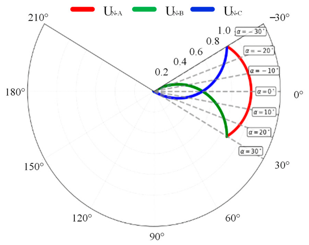
For phases B and C, in $\alpha \in (0°,30°)$, $\cos (\alpha +120°)$ and $\cos (\alpha -120°)$ are usually negative values, causing $\Delta {\dot{U}}_{N-B}>0$ and $\Delta {\dot{U}}_{N-C}>0$ to exhibit a voltage rise.

A comparison of Equation (7) with Equations (8) and (9) shows that the difference between the voltage magnitude change of phase A and those of phases B and C arises from two factors. First, phase A additionally contains the phase conductor voltage-drop component, which is absent in phases B and C. Second, the phase A projection $|\cos (\alpha )|$ of the neutral-conductor component is greater than the projections $|\cos (\alpha \pm 120°)|$ of the B and C phases. As shown in Figure 3, the change in $\alpha$ within $(–30°,30°)$ has an impact on the three-phase projections. It clearly shows that the phase A component always dominates, while the phase B and phase C components exhibit opposite monotonic trends. Considering both factors, and given that the phase conductor and neutral-conductor impedances are similar in engineering practice, the voltage-drop magnitude of the event phase can be four to six times that of the non-event phases (depending on the impedance ratio of the line).

2.3. Other Meter Boxes

After clarifying the cross-phase coupling effect within the same meter box, the propagation characteristics of an event to different meter boxes are further examined. For customers connected to different meter boxes, such as customer $c_k$ or customer $b_m$ in Figure 1, their voltage responses depend on their electrical distances between the event-source customer $a_i$. When a load switching event occurs at customer $a_i$, resulting in a change $\Delta I_i$ in the operating current, the voltage fluctuations observed at different locations in the network are as follows:

$$\Delta U_i=\Delta I_i\cdot (Z_{12}+Z_{10}+Z_7+Z_1)$$

(10)

$$\Delta U_1=\Delta I_i\cdot (Z_{12}+Z_{10}+Z_7)$$

(11)

$$\Delta U_m=\Delta I_i\cdot (Z_{12}+Z_{10})$$

(12)

$$\Delta U_k=\Delta I_i\cdot Z_{12}$$

(13)

$$\left|\Delta U_i\right|\approx \left|\Delta U_j\right|>\left|\Delta U_m\right|>\left|\Delta U_k\right|$$

(14)

where $\Delta U_i$, $\Delta U_1$, $\Delta U_m$, $\Delta U_k$ respectively correspond to the voltage change values of customers $a_i$, $a_1$, $b_m$, and $c_k$ in Figure 1.

Equations (10)–(14) directly show the inverse relationships between the voltage response magnitude and the electrical distance between meter boxes: As the electrical distance increases, the common impedance path becomes shorter, resulting in a smaller response magnitude. The physical essence of this phenomenon lies in the differences of the common impedance paths in the distributed impedance network. Therefore, same-phase customers within the same meter box exhibit highly consistent responses, whereas customers connected to different meter boxes show quantifiable response attenuation as the electrical distance increases. This provides an observable basis for identifying customer–meter box relationship identification.

2.4. Voltage Response Examples

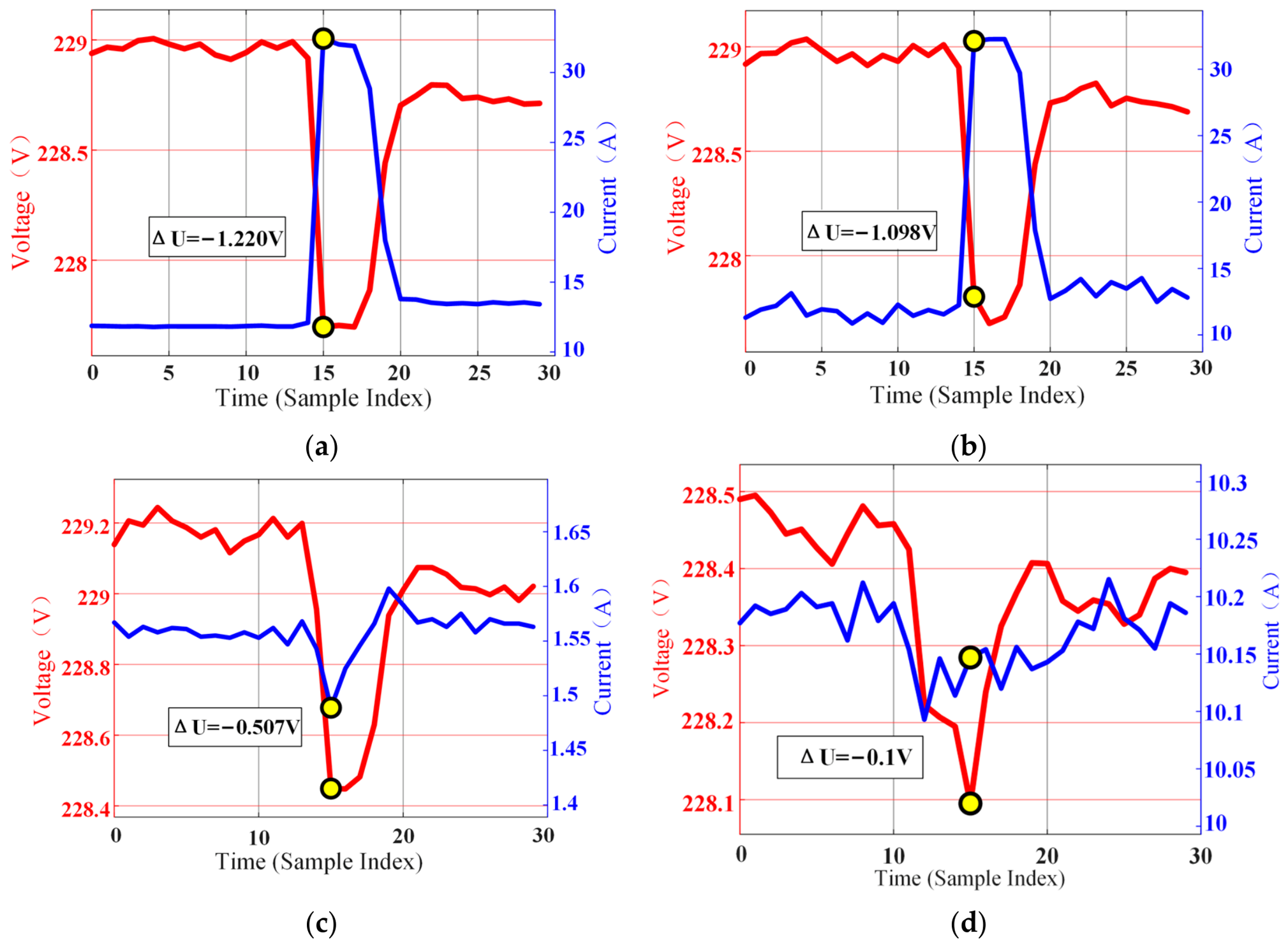
Figure 4 shows the effect of a load-switching event at a phase A customer in a meter box on the voltages of customers at different locations. The sampling interval of the root-mean-square (RMS) sequences of current and voltage in the figure is 20 ms, enabling accurate detection of voltage changes. When a phase A customer in Meter Box 1 experiences a current change of approximately 11 A, a significant voltage drop of approximately 1.22 V is observed at this customer. Other customers in the same meter box experience significant voltage drop of approximately 1.1 V in the same direction. Customers connected to the same branch but located in different meter boxes experience synchronous voltage drop in the same direction, with the magnitude attenuated to approximately 0.5 V. For customers connected to different branches and located in different meter boxes, the common impedance path is very short. Therefore, the observed voltage fluctuations are the weakest, with synchronous voltage drops in the same direction attenuated to approximately 0.1 V.

In conclusion, this section reveals the dynamic response characteristics of load switching events in LVDNs. The high consistency of customer responses within the same meter box and the cross-phase coupling effect provide a basis for the subsequent design of the customer–meter box relationship identification algorithm.

3. Two-Stage Method for Customer–Meter Box Relationship Identification

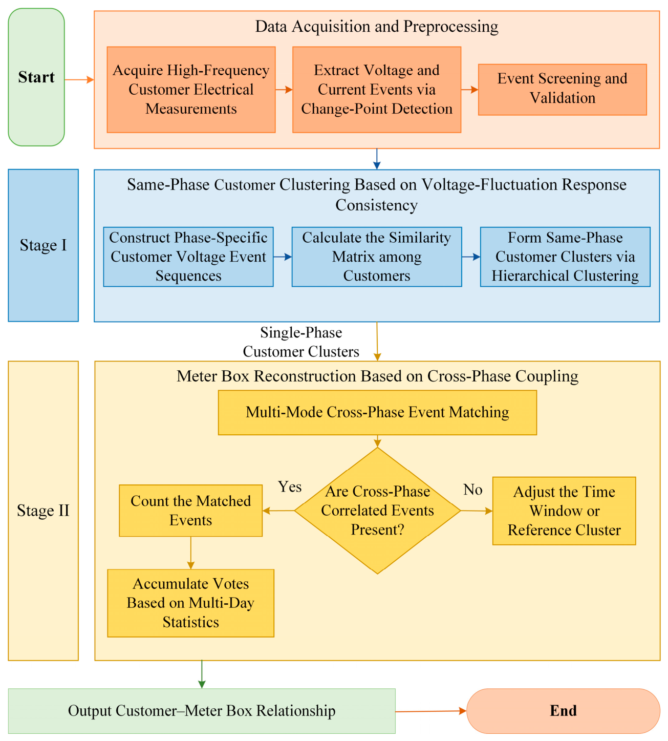
To identify the customer–meter box relationships, based on dynamic response mechanism described above, this paper divides the identification process into two stages: In the first stage, same-phase customers are clustered based on the high consistency of customer responses within the same meter box. Thus, customers in LVDN containing $N$ meter boxes are divided into 3N clusters. In the second stage, the $3N$ clusters are combined into N meter box clusters based on the cross-phase coupling effect. The customer–meter box relationships are then identified. The overall process is shown in Figure 5.

3.1. Clustering of Same-Phase Customers Within the Same Meter Box Based on Response Consistency

Based on the theoretical analysis in Section 1, the voltage responses of single-phase customers within the same meter box to any load switching event are highly consistent. Therefore, a similarity-based method can be used to determine the meter box assignment of single-phase customers. Considering that voltage event sequences consist of discrete timestamp–magnitude pairs, conventional continuous time-series analysis methods are no longer applicable. Therefore, in this section, a dedicated similarity measurement method is designed.

3.1.1. Similarity Measurement of Event Sequences

Define the voltage event sequence of customer $i$ as a time-ordered set:

$$E_i=\{e_{i,1},e_{i,2},\dots ,e_{i,n_i}\}$$

(15)

where $e_{i,k}$ represents the $k$-th event, which includes the time $t_{i,k}$ and the voltage change magnitude $\Delta V_{i,k}$. $n_i$ is the total number of events of customer $i$, and $t_{i,1}<t_{i,2}<\dots <t_{i,n_i}$, this sequence is equivalent to the combination of timestamp vector $T_i={[t_{i,1},t_{i,2},\dots ,t_{i,n_i}]}^T$ and amplitude vector $V_i={[\Delta V_{i,1},\Delta V_{i,2},\dots ,\Delta V_{i,n_i}]}^T$.

In this section, a time-window-based matching method is used to calculate the similarity between two event sequences, and the matching time window is set to $T_1=\delta s$.

The steps for calculating similarity are as follows:

(1)

Event search within the time window. For each event $e_{i,k}$ of customer $i$, candidate events that satisfy the time synchronization constraint are searched for in event sequence $E_j$ of customer $j$:

$$C_{j,k}=\{e_{j,m}\mid |t_{i,k}-t_{j,m}|\le \delta \}$$

(16)

where $C_{j,k}$ represents the candidate set. If it is empty, no matching event exists.

(2)

Magnitude similarity evaluation and event matching. To avoid the bias of multiple matches, only the event with the highest magnitude similarity is selected as the optimal match for each $e_{i,k}$. For a nonempty candidate set $C_{j,k}$, calculate the magnitude similarity between each candidate event and $e_{i,k}$.

$$\mathrm{sim}(v_{i,k},v_{j,m})=\exp \left(-{\displaystyle \frac{{(\Delta V_{i,k}-\Delta V_{j,m})}^2}{2{\sigma }^2}}\right)$$

(17)

where $\sigma$ is the magnitude tolerance parameter, $\Delta V_{i,k}$ and $\Delta V_{j,k}$ are respectively the voltage change magnitudes of the corresponding events for customer $i$ and customer $j$. This measurement is based on the $\Delta V_{j,l}$ Gaussian kernel function [30]. The smaller the magnitude difference, the closer the similarity is to 1.

If the magnitude similarity is greater than $S_{th}$, the match is considered successful. The threshold of $S_{th}$ is selected based on the analysis of actual data to ensure that only highly similar event pairs are considered valid matches.

(3)

Matching rate calculation. This step is based on the results of step (2) and calculates the matching rate:

$$r_{i\to j}={\displaystyle \frac{M_{i\to j}}{N_i}}$$

(18)

where $M_{i\to j}$ represents the total number of optimal matching events from customer $i$ to customer $j$, and $N_i$ represents the total number of events of customer $i$. Since the number of events in the two sequences may be different, the bidirectional matching rates $r_{i\to j}$ and $r_{j\to i}$ should be calculated separately.

(4)

Comprehensive similarity calculation. The final similarity is calculated using the harmonic mean:

$$S(E_i,E_j)={\displaystyle \frac{2r_{i\to j}{r}_{j\to i}}{r_{i\to j}+r_{j\to i}}}$$

(19)

This measure ensures the symmetry of the similarity, $S(E_i,E_j)=S(E_j,E_i)$, and is more sensitive to lower matching rates. The final similarity approaches 1 only when the bidirectional matching rates are both very high, which is consistent with the high bidirectional similarity between the voltage event sequences of same-phase customers within the same meter box.

In the same-phase clustering stage described in this section, a short matching window of $T_1=3 \mathrm{s}$ is adopted. For each voltage event recorded by one customer, candidate events from another customer are searched for within $\pm 3 \mathrm{s}$. The final event correspondence is then determined by combining this temporal constraint with the magnitude similarity. This short window accommodates limited event-level timestamp discrepancies while preserving the temporal discriminability required for same-phase customer clustering.

3.1.2. Hierarchical Clustering and Data-Driven Meter-Box Count

Based on Section 3.1.1, an $N\times N$ similarity matrix $S$ is calculated, where $N$ represents the number of customers, and element $S_{ij}=S(E_i,E_j)$ represents the similarity of the voltage event sequences between customer $i$ and customer $j$. To meet the distance metric requirement of the clustering algorithm, the similarity matrix is first converted into a distance matrix:

$$D_{ij}=1-S_{ij},i,j=1,2,\dots ,N$$

(20)

where element $S_{ij}=S(E_i,E_j)$ in the distance matrix represents the similarity of voltage event sequences between customers.

Subsequently, the agglomerative hierarchical clustering algorithm was employed to group the customers [31].

The steps are as follows:

(1)

Initialize the cluster set $\mathcal{C}=C_1,C_2,\dots ,C_N$, where each cluster $C_i=i$ contains only one customer.

(2)

The closest pair is repeatedly merged until the complete dendrogram is obtained.

Calculate the distances between all current cluster pairs using the average linkage method [32].

$$d(C_p,C_q)={\displaystyle \frac{1}{\left|C_p\right|\left|C_q\right|}}{\displaystyle \sum _{i\in C_p}{\displaystyle \sum _{j\in C_q}{D}_{ij}}}$$

(21)

$$(C_p^{*},C_q^{*})=\arg {\min }_{C_p,C_q\in \mathcal{C}}d(C_p,C_q)$$

(22)

$$C_{\mathrm{new}}=C_p^{*}\cup C_q^{*}$$

(23)

where $C_p$ and $C_q$ are the closest pair of clusters, $C_{\mathrm{new}}$ is the merged cluster, $d(C_p,C_q)$ is the distance between clusters $C_p$ and $C_q$. $\left|C_p\right|$ and $\left|C_q\right|$ are the number of customers within the clusters. After each merging operation, the corresponding linkage distance and cluster configuration are recorded to construct the complete hierarchical clustering dendrogram. The merging process is continued until the complete dendrogram is obtained, and the appropriate number of clusters is subsequently determined using a clustering-validity criterion.

(3)

Let the dendrogram of phase $p$ be cut into $K$ clusters, where $K$ is searched over a candidate range from 2 to $K_{\max }$. Let the numbers of customers in phases A, B, and C be $M_A,M_B,M_C$ respectively. Since phases A, B, and C are clustered using the same candidate number of meter boxes $K$, $K_{\max }$ satisfies $K_{\max }={\min }_{p\in \{A,B,C\}}(M_p-1)$. The upper bound is determined by the mathematical applicability of the silhouette coefficient.

The phase-specific distance matrix is obtained from the phase-specific similarity matrix using the same transformation $D=1-S$ defined above. For customer $i$ belonging to cluster $C_i$, the average intra-cluster distance is defined as

$$a^{(p)}(i)={\displaystyle \frac{1}{\left|C_i\right|-1}}{\displaystyle \sum _{j\in C_i,j\ne i}{D}_{ij}^{(p)}}(\left|C_i\right|>1)$$

(24)

The minimum average distance from customer i to any other cluster is defined as

$$b^{(p)}(i)={\min }_{C_q\ne C_i}\left\{{\displaystyle \frac{1}{\left|C_q\right|}}{\displaystyle \sum _{j\in C_q}{D}_{ij}^{(p)}}\right\}$$

(25)

Accordingly, the silhouette coefficient of customer i is defined as

$$s^{(p)}(i)=\left\{\begin{array}{c}{\displaystyle \frac{b^{(p)}(i)-a^{(p)}(i)}{\max \{a^{(p)}(i),b^{(p)}(i)\}}},\left|C_i\right|>1\\ 0,\left|C_i\right|=1\end{array}\right.$$

(26)

A candidate partition is allowed to contain singleton clusters because a meter box may contain only one customer on a particular phase. For a singleton cluster, the silhouette coefficient of the corresponding customer is conventionally assigned a value of zero since within-cluster compactness cannot be evaluated from a single sample. Therefore, singleton clusters are retained rather than excluded from the candidate partitions. A value of $s^{(p)}(i)$ closer to 1 indicates a higher degree of matching between the customer and the current cluster, as well as a clearer separation from other clusters.

The average silhouette coefficient for phase p under candidate cluster number $K$ is

$$S{C}_p(K)={\displaystyle \frac{1}{M_p}}{\displaystyle \sum _{i=1}^{M_p}{s}^{(p)}}(i)$$

(27)

Because phases A, B, and C correspond to the same physical set of meter boxes, the phase-specific indices are combined into a three-phase validity index:

$$S{C}_{avg}(K)={\displaystyle \frac{{\sum }_{p\in \{A,B,C\}}{M}_{p}S{C}_p(K)}{{\sum }_{p\in \{A,B,C\}}{M}_p}}$$

(28)

The estimated number of meter boxes is selected as the candidate number that maximizes the three-phase average silhouette coefficient:

$$\widehat{N}=\arg {\max }_{2\le K\le K_{\max }}S{C}_{\mathrm{avg}}(K)$$

(29)

A high silhouette value indicates that customers are simultaneously compact within their assigned groups and well separated from customers in other groups. Intuitively, an underestimated $K$ may merge customers belonging to different meter boxes, leading to larger within-cluster dissimilarities. Conversely, an overestimated $K$ may unnecessarily split customers associated with the same meter box, making some clusters less well separated. The maximum of $S{C}_{\mathrm{avg}}(K)$ thus provides a data-driven criterion for selecting the meter-box number without relying on topology records. The corresponding dendrogram cut at $K=\widehat{N}$ is subsequently used as the input to the cross-phase matching stage.

The proposed procedure assumes that the phase label of each customer is available and sufficiently reliable. The silhouette coefficient itself is a generic clustering-validity index; however, in the present framework it is evaluated on phase-specific customer sets.

3.2. Customer–Meter Relationship Identification Based on Cross-Phase Cluster Merging

After same-phase customer clustering is completed, the second stage further combines the single-phase clusters into complete three-phase meter box clusters. When a significant current switching event occurs within a driving-phase cluster, the response clusters on the other phases within the same meter box show strong coupling through the shared neutral-conductor impedance. Therefore, significant voltage responses can be observed simultaneously. In contrast, cross-phase response clusters in different meter boxes have shorter common impedance paths, and their voltage responses are smaller than those within the same meter box. These response magnitudes are below the event detection threshold and therefore cannot be detected. Therefore, by counting the number of current–voltage event pairs that satisfy the time synchronization constraint, the strength within a cluster correlation can be quantified.

3.2.1. Synchronization Matching Based on Cross-Phase Events

A matching count function $N_{match}(E_{I,i}^{{\varphi }_d},E_{U,j}^{{\varphi }_r})$ is defined to count the total number of successfully matched event pairs between the driving current sequence and the response voltage sequence. It then maximizes the number of matched events by searching for the optimal time shift ${\tau }_{opt}$.

Here, $E_{I,i}^{{\mathsf{\varphi }}_d}$ refers to the set of current events of the $i$-th customer cluster on phase ${\mathsf{\varphi }}_d$, and each event is characterized by its occurrence time $t$ and current change magnitude $\Delta I$. $E_{U,j}^{{\mathsf{\varphi }}_r}$ refers to the set of voltage events recorded by the $j$-th customer cluster on phase ${\mathsf{\varphi }}_r$, and each event is characterized by its occurrence time $t$ and current change magnitude $\Delta U$.

The calculation process is shown in Algorithm 1:

Algorithm 1: Counting matched events between cross-phase clusters.

$\begin{array}{l}Function\mathrm{CountMatchedEvents}(E_I,E_U)\\ \mathrm{where}{E}_I={\{(t_{I,i},\Delta I_i)\}}_{i=1}^m,E_U={\{(t_{U,j},\Delta U_j)\}}_{j=1}^n\\ //Driving\text{-}PhaseCurrentEventSequence{E}_I\\ //Response\text{-}PhaseVoltageEventSequence{E}_U\\ \mathrm{Set}\mathrm{offsetRange}=[-T_2,T_2]\\ //DefinetheSearchRangeforSystematicTimeOffsets\\ \mathrm{Set}\mathrm{maxMatchCount}=0\\ for each\tau \in \mathrm{offsetRange}do\\ \hspace{1em}\mathrm{Set}\mathrm{currentMatchCount}=0\\ \hspace{1em}\mathrm{Set}\mathrm{responderMatched}=\varnothing \\ \hspace{1em}foreachi=1\mathrm{to}mdo\\ \hspace{1em}\hspace{1em}foreachj=1\mathrm{to}ndo\\ \hspace{1em}\hspace{1em}\hspace{1em}ifj\notin \mathrm{responderMatched}then\\ \hspace{1em}\hspace{1em}\hspace{1em}\hspace{1em}if|t_{U,j}-(t_{I,i}+\tau )|\le {\epsilon }_{t}then\\ \hspace{1em}\hspace{1em}\hspace{1em}\hspace{1em}\hspace{1em}\mathrm{Set}\mathrm{currentMatchCount}=\mathrm{currentMatchCount}+1\\ \hspace{1em}\hspace{1em}\hspace{1em}\hspace{1em}\hspace{1em}\mathrm{Add}j\mathrm{to}\mathrm{responderMatched}\\ \hspace{1em}\hspace{1em}\hspace{1em}\hspace{1em}\hspace{1em}break\\ if\mathrm{currentMatchCount}>\mathrm{maxMatchCount}then\\ \mathrm{Set}\mathrm{maxMatchCount}=\mathrm{currentMatchCount}\\ return\mathrm{maxMatchCount}\end{array}$

The algorithm addresses the time synchronization constraint by setting a matching time window $T_2$ to accommodate second-scale deviations in event timestamps and determining the optimal time shift ${\tau }_{opt}$ to correct possible clock desynchronization between different devices. This sequence-level correction is introduced to compensate for possible clock desynchronization between different metering devices.

The “maxMatchCount” returned by the algorithm represents the number of matched events between two clusters. For customer clusters within the same meter box, the response voltage magnitudes are usually significantly higher than the threshold and are highly aligned within the time window. Therefore, the number of matched events increases significantly. In contrast, response voltage magnitudes of clusters in different meter boxes are weak and are often below the extraction threshold of $U_{th}$, or they are not temporally synchronized, resulting in a low number of matched events. This difference ensures that the number of matched events between clusters within the same meter box is the largest.

3.2.2. Meter Box Topology Modeling Based on Multiple Verification Mechanisms

To ensure robustness and accuracy under complex operating conditions, this section proposes a meter box topology reconstruction method that combines multi-mode cross-validation, voting quantification, and a greedy heuristic algorithm. An uncertainty-aware confidence screen is further introduced so that weak or nearly tied assignments can remain unresolved instead of being forced into the reconstructed topology.

• Multi-Mode Cross-Validation and Voting Quantification

To avoid incorrect associations caused by poor single-phase data quality or sparse events, a set of verification mode $\Omega =\{A\to BC,B\to AC,C\to AB\}$ is defined, which represents the matching process that use the current events of phase A, phase B, and phase C as the driving events, respectively, and the voltage events of the other two phases as the responses.

A voting mechanism is introduced to eliminate the interference of random noise. The voting horizon is set to $D$ days. For any possible cross-phase cluster combination $(C_i^A,C_j^B,C_k^C)$ (where $C_i^A$ represents the $i$-th customer cluster of phase A, and so on), define the cumulative matching votes $S_{ijk}$ as

$$S_{ijk}={\displaystyle \sum _{d=1}^T{\displaystyle \sum _{m\in \Omega }{N}_{match}(C_i^A,C_j^B,C_k^C|d,m)}}$$

(30)

where represents the total number of successfully matched current–voltage event pairs within the three-phase cluster combination on the $d$-th day and in the $m$-th verification mode.

The correct meter box relationships continuously accumulate a high number of votes during the observation period, while false associations caused by occasional noise are smoothed and filtered out.

2.

Greedy Heuristic Algorithm Based on Vote Priority

To meet the timeliness requirements of engineering applications, this paper develops a greedy heuristic algorithm based on vote priority (GH-VP). The core idea of GH-VP is to sequentially select meter box combinations in descending order of their vote counts while ensuring that each single-phase cluster is assigned only once. The detailed procedure is presented in Algorithm 2. First, the accepted-combination set ${\Omega }^{*}$ and the accepted-index sets ${\Lambda }_A,{\Lambda }_B,{\Lambda }_C$ are initially empty. The manual-review set $M$ and the review-reserved index sets $R_A,R_B,R_C$ are also initialized as empty sets. The algorithm then enumerates all $N^3$ possible three-phase cluster combinations $(C_i^A,C_j^B,C_k^C)$, calculates the cumulative vote count $S_{ijk}$ for each combination, and sorts all candidate combinations in descending order of their vote counts to form an ordered candidate list.

Algorithm 2: Greedy heuristic algorithm based on vote priority.

$\begin{array}{l}Input:Totalnumberofidentifiedsingle\text{-}phaseclustersN;allpossiblethree\text{-}phaseclustercombinationsand\\ theircumulativevotecounts\left\{S_{ijk}\right\};thresholds{V}_{min},\Delta V_{min},and{C}_{min}\\ Output:Finalacceptedmeterboxcombinations{\Omega }^{*};manual\text{-}reviewsetM\\ 1: {\Lambda }_A=\varnothing ,{\Lambda }_B=\varnothing ,{\Lambda }_C=\varnothing //Initializetheaccepted\text{-}indexsetsforthephaseA,B,andCclusters\\ \phantom{1: }{R}_A=\varnothing ,R_B=\varnothing ,R_C=\varnothing //Initializethereview\text{-}reservedindexsetsasanemptyset\\ 2: {\Omega }^{*}=\varnothing //Initializetheacceptedcombinationsasanemptyset\\ \phantom{2: }M=\varnothing //Initializethemanual\text{-}reviewsetasanemptyset\\ 3: L=Sor{t}_{Descending}(\{S_{ijk}\})//Calculatethevotecountsofallpossiblecombinationsandsortthemindescendingorder\\ 4: \mathbf{for}(i,j,k)\in L \mathbf{do}\\ 5: \mathbf{if} i\in \left(\Lambda A\cup RA\right)orj\in \left(\Lambda B\cup RB\right)ork\in \left(\Lambda C\cup RC\right) \mathbf{then}\\ //Checkwhetherallthreeclustersinthecurrentcombinationareunassignedcontinue\\ \hspace{1em}\hspace{1em}\hspace{1em}\mathbf{\text{end if}}\\ 6: V1=S_{ijk}\\ 7: Q_{ijk}=\left\{\left(p,q,r\right)\in L\backslash \left\{\left(i,j,k\right)\right\}:p=iorq=jorr=k\}\right.\\ 8: V_2=0ifQ=\varnothing ;\\ \hspace{1em}\hspace{1em}\hspace{1em}otherwise{V}_2=max\left\{S\left(p,q,r\right):\left(p,q,r\right)\in Q_{ijk}\right\}\\ 9: \Delta V=V_1-V_2\\ \phantom{9: }C=\Delta V/max\left(V_1,1\right)\\ 10:\mathbf{if}V1\ge Vminand\Delta V\ge \Delta VminandC\ge Cminthen\\ 11: {\Omega }^{*}={\Omega }^{*}\cup \{i,j,k\}\\ 12: {\Lambda }_A={\Lambda }_A\cup \left\{i\right\};{\Lambda }_B={\Lambda }_B\cup \left\{j\right\};{\Lambda }_C={\Lambda }_C\cup \left\{k\right\}\\ 13: \hspace{1em}\hspace{1em}else\\ 14: M=M\cup \left\{\left(i,j,k,V_1,\Delta V,C,failedcriterion\right)\right\}\\ 15: R_A=R_A\cup \left\{i\right\};R_B=R_B\cup \left\{j\right\};R_C=R_C\cup \left\{k\right\}\\ 16: \mathbf{end} \mathbf{if}\\ 17: ifSize\left(\Omega *\right)=Nthenbreakendif\\ 18: \mathbf{end} \mathbf{for}\\ 19: return\Omega *,M\end{array}$

During the greedy selection stage, the candidates in the ordered list L are examined in descending order of their cumulative vote scores. A candidate that combines the $i$ -th phase A cluster, the $j$-th phase B cluster, and the $k$-th phase C cluster is considered only if $i$ is not contained in either the accepted phase A index set or the review-reserved phase A index set, $j$ is not contained in either corresponding phase B set, and $k$ is not contained in either corresponding phase C set. Thus, none of the candidate"s three clusters may have been accepted or reserved for manual review previously. A candidate that violates this condition conflicts with an earlier decision and is skipped without changing any set. An eligible candidate is not accepted merely because it is currently the highest-ranked candidate. It must also satisfy the minimum-support, absolute-margin, and normalized-margin criteria. If all three criteria are satisfied, the candidate is added to the accepted-combination set ${\Omega }^{\ast }$, and its three cluster indices are added to the corresponding accepted-index sets. If any criterion fails, the candidate is added to the manual-review set $M$, and its three cluster indices are added to the review-reserved sets. The procedure terminates when $N$ combinations have been accepted or when all candidates in $L$ have been examined. Consequently, the selective GH-VP procedure always produces a conflict-free set of automatic assignments but may accept fewer than $N$ meter-box combinations when the available evidence is insufficient.

The one-to-one assignment constraint prevents a single-phase cluster from being used in more than one accepted combination, but it does not quantify the ambiguity of an assignment. Consider an eligible three-phase candidate, and let $V_1=S_{ijk}$ denote its cumulative vote score over the prescribed voting horizon. Its competing set $Q_{ijk}$ contains every other candidate $\left(p,q,r\right)$ in $L$ that shares at least one constituent cluster with the current candidate; that is, $p=i,q=j,r=k$. Let $V_2$ be the largest cumulative vote score among the candidates in $Q_{ijk}$. If $Q_{ijk}$ is empty, $V_2$ is set to zero. The absolute vote margin is defined as $\Delta V=V_1-V_2$, and the normalized vote margin is defined as $C=\Delta V/max\left(V_1,1\right)$.

A normalized vote margin close to zero indicates a near tie, whereas a larger value indicates clearer separation from the strongest conflicting candidate. Because the normalized margin alone does not measure the amount of supporting evidence, automatic acceptance requires $V_1\ge V_{min},\Delta V_1\ge \Delta V_{min}$ and $C\ge C_{min}$ simultaneously. If all three inequalities hold, the candidate is accepted, and its three indices are locked in the accepted-index sets. Otherwise, the candidate, its decision statistics $\left(V_1,\Delta V,C\right)$, and the failed criterion or criteria are recorded in $M$. Its three indices are then placed in the review-reserved sets, ensuring that no later candidate containing any of those clusters can be assigned automatically. The thresholds $V_{min},\Delta V_{min}$, and $C_{min}$ are jointly selected using an independent validation set. For each threshold combination, the complete sequential assignment procedure is executed, and both the exact-triplet accuracy among automatically accepted candidates and the automatic acceptance rate are evaluated.

4. Case Analysis

4.1. Experimental Setup

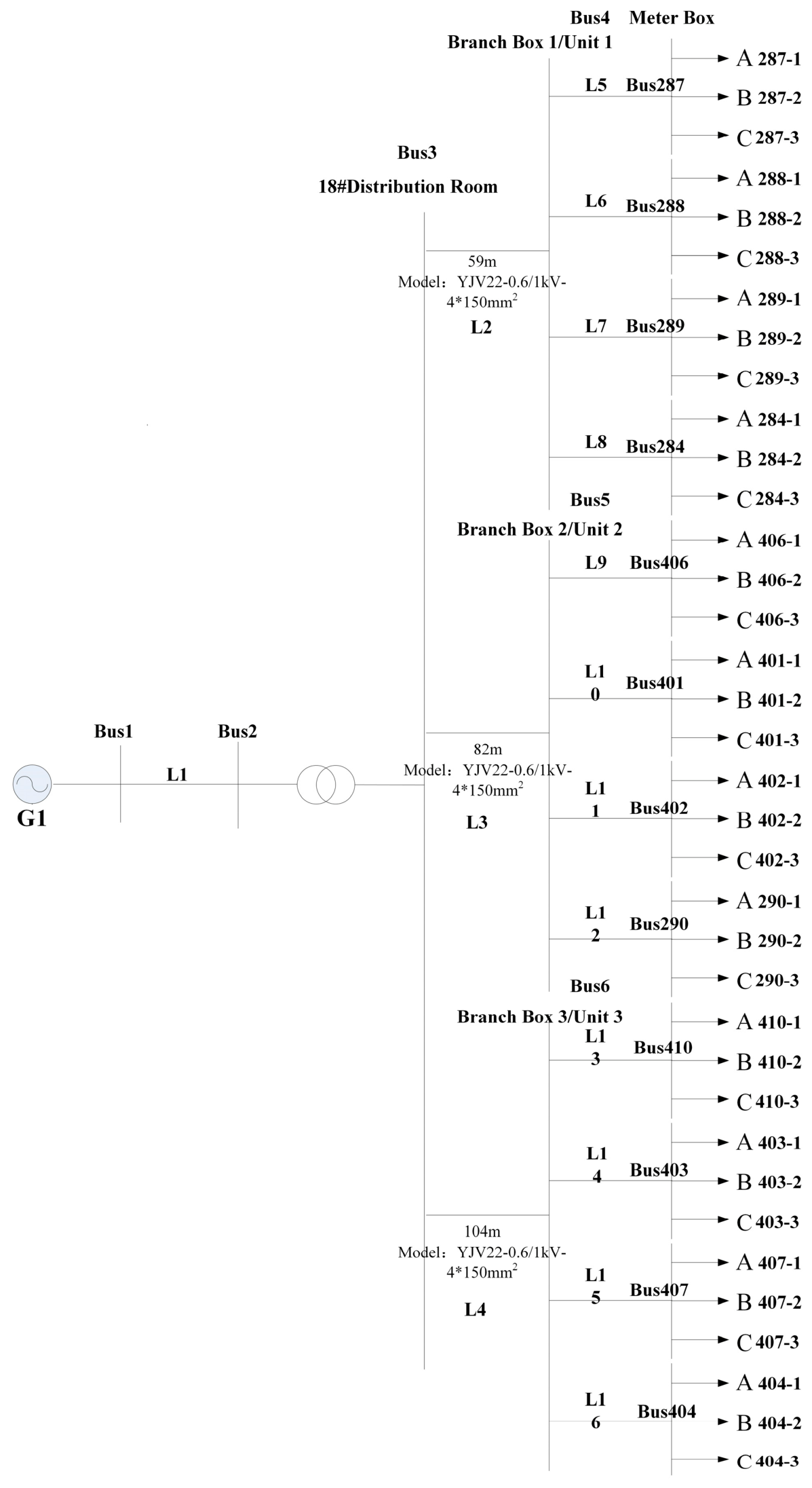
As shown in Figure A1, a three-phase four-wire residential LVDN in Nanjing was used as the test system, comprising 12 m boxes and 144 customer nodes. Dual-chip smart meters sample electrical quantities at 20 ms intervals and capture pre- and post-event data, which are uploaded to the master station every 15 min via HPLC. The 20 ms interval is used only for local transient detection and does not require meter-to-meter synchronization. Inter-meter association uses source-event timestamps with 1 s resolution, while the 15 min interval is only the upload batch period; preserved source timestamps therefore decouple communication latency from event time. Customer–meter-box relationships and phase assignments were obtained through manual verification and HPLC phase information and used as benchmark labels.

4.2. Analysis of Thresholds Selection

4.2.1. Voltage Event Threshold

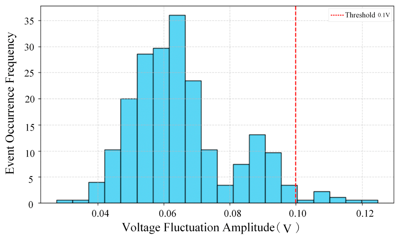
In this study, stationary sequences without significant change points were selected as noise samples, and the voltage fluctuations in 10 LVDNs in Nanjing, involving approximately 500 customers, were analyzed. The measurement data were acquired at 20 ms intervals using an RN2026 metering chip manufactured by Renergy Micro-Technologies. The differences in the voltage RMS sequences were calculated, and the statistical results are shown in Figure 6. For the present internal reconstruction, the empirical 99th percentile is taken as $Q_{0.99}(\left|\Delta U_{noise}\right|)\approx 0.10\mathrm{V}$.

4.2.2. Current Event Threshold

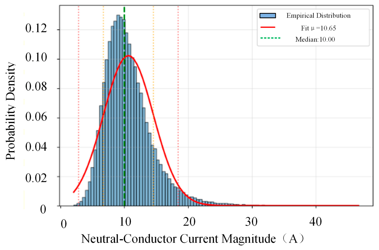
After selecting the voltage event threshold, it is necessary to ensure that current events within the same meter box can trigger voltage responses that exceed this threshold. As derived earlier, with the same current disturbance, the same-phase voltage change is greater than the cross-phase response. To ensure that all target customers can detect the event, it is necessary to derive the required minimum current threshold based on the response of the non-event phases. For typical LVDN parameters, to ensure that the cross-phase response of a non-event phase is no less than 0.1 V, according to Equations (8) and (9), the required current threshold depends on the neutral-conductor impedance and the neutral-point displacement angle $\alpha$. Because their empirical distributions are unavailable, both parameters were modeled using bounded uniform distributions over their engineering ranges. Specifically, the common neutral-conductor impedance was modeled as $Z_N~U(10,50) \mathrm{m}\Omega$, and the neutral-point displacement angle was modeled as ${\theta }_N~U(-30°,30°)$. The two parameters were sampled independently, and ${10}^5$ Monte Carlo samples were generated. The Monte Carlo analysis was used to characterize the current magnitude required to produce an observable cross-phase voltage response under uncertainty conditions in the neutral-conductor parameters, and the results are shown in Figure 7.

Combined with the above analysis and the practical residential loads listed in

Table 1. Rated power and current characteristics of typical residential electrical equipment.

Appliance Type	Rated Power (W)	Rated Current (A)
Electric Water Heater	2000–3000	9.1–13.6
Induction Cooker	2000–2500	9.1–11.4
Air Conditioner	1800–3000	8.2–13.6
Electric Rice Cooker	500–1500	2.3–6.8
Hair Dryer	1800–2000	8.2–9.1

, electric water heaters, induction cookers, air conditioners, and hair dryers typically draw 8.2 to 13.6 A, whereas electric rice cookers are generally below 8 A (2.3 to 6.8 A). Therefore, 8 A is selected as a conservative lower threshold for current-event screening. This threshold retains switching events from common high-power appliances that are more likely to produce observable cross-phase responses, while excluding weaker events that may be missed or lead to unstable cross-phase matching.

4.2.3. Magnitude Similarity Threshold

After temporal matching, the pooled magnitude-similarity scores are inspected. When low- and high-similarity modes are clearly separated, the cutoff $S_{th}$ is selected near the lower tail of the high-similarity group, subject to engineering bounds. If the distribution is not clearly bimodal, the last validated threshold is retained. A one-dimensional density estimate is first constructed from all candidate-pair similarity scores. For the investigated LVDN, the low- and high-similarity modes are separated by an inter-mode density minimum at approximately $s_v=0.56$. The pooled scores are therefore partitioned into the low-similarity and high-similarity components, $S_L$ and $S_H$, according to the rule. With $p=0.05$, the lower-tail quantile of the high-similarity component is $Q_{0.05}(S_H)\approx 0.80$.

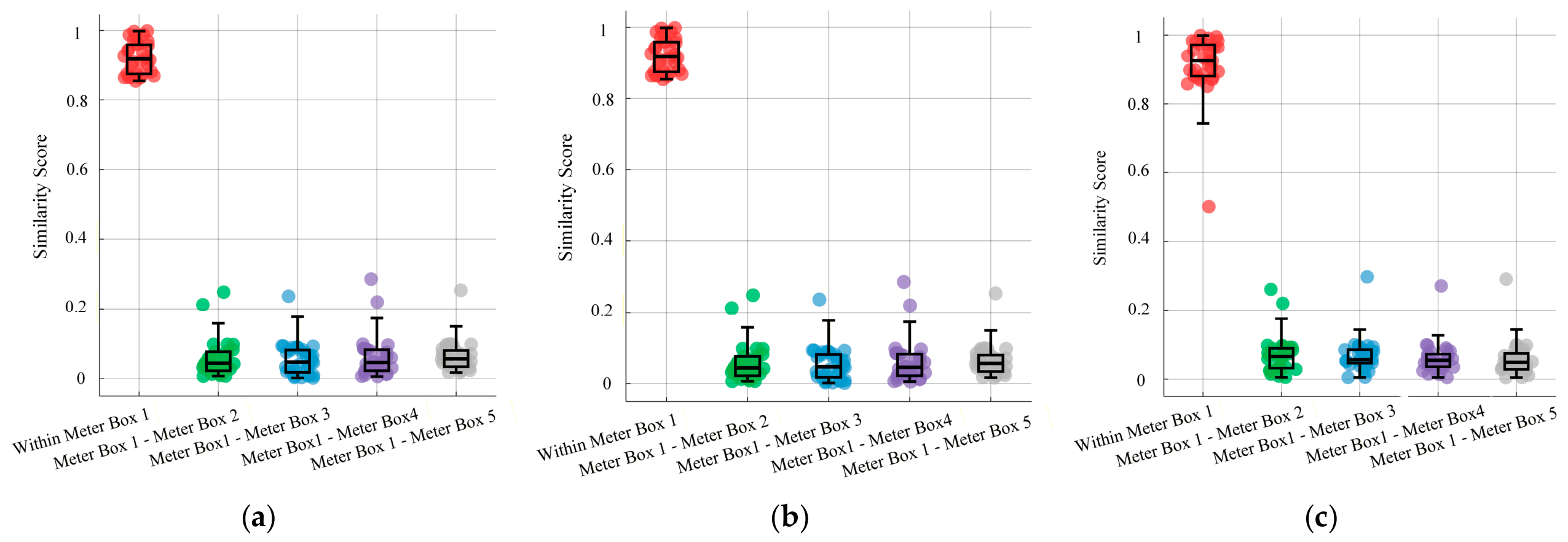
As shown in Figure 8, the similarity distribution of customer voltage event sequences within the meter box and between different meter boxes exhibits a significant bimodal pattern.When two customers belong to the same meter box, their similarity remains above 0.8; whereas when customers belong to different meter boxes, the similarity is concentrated around 0.1.

Figure 8. Similarity comparison analysis diagram between the inside of the meter box and between meter boxes: (a) comparison of within-box and between-box similarities for phase A customers; (b) comparison of within-box and between-box similarities for phase B customers; (c) comparison of within-box and between-box similarities for phase C customers.

Figure 8. Similarity comparison analysis diagram between the inside of the meter box and between meter boxes: (a) comparison of within-box and between-box similarities for phase A customers; (b) comparison of within-box and between-box similarities for phase B customers; (c) comparison of within-box and between-box similarities for phase C customers.

4.2.4. Voting Horizon Threshold

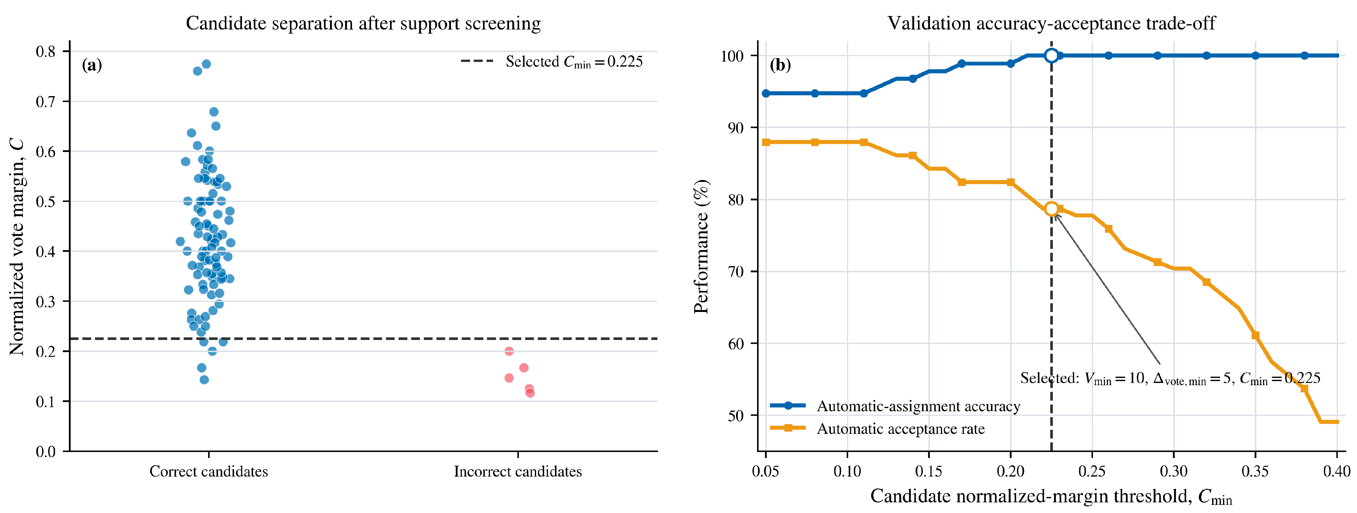
With the event thresholds fixed as established in Section 4.2.1 and Section 4.2.2, for the leading vote $V_1$ and the strongest conflicting vote $V_2$, the absolute and normalized margins were defined as ${\Delta }_{\mathrm{vote}}=V_1-V_2$ and $C={\Delta }_{\mathrm{vote}}/\max (V_1,1)$, respectively. As shown in Figure 9, the selected thresholds $V_{\min }=10, {\Delta }_{\mathrm{vote},\min }=5$ and $C_{\min }=0.225$ achieved 100% accuracy for automatically accepted assignments while retaining an acceptance rate of 78.7%.

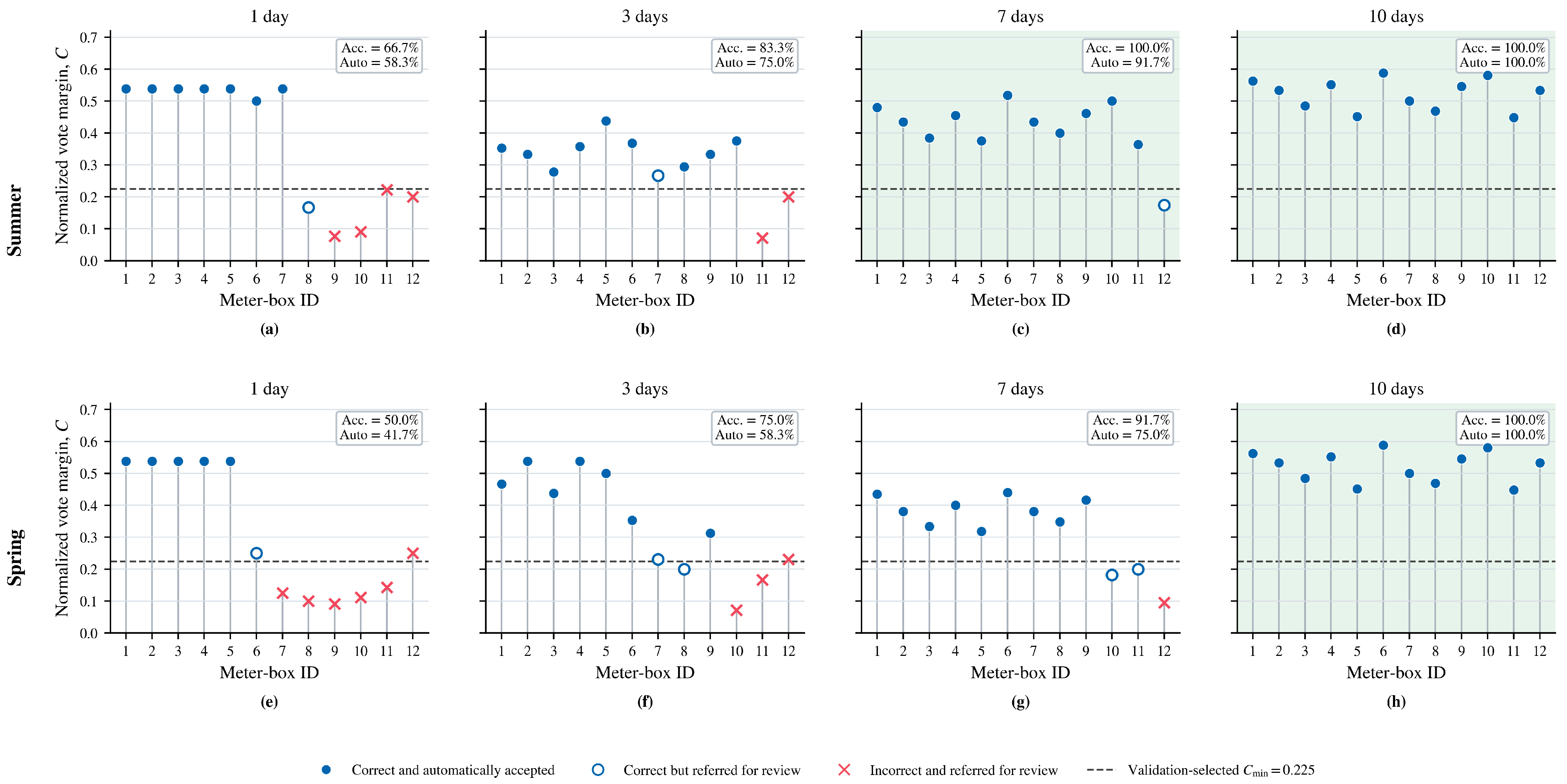
Using these thresholds, voting horizons of 1, 3, 7, and 10 days were evaluated by rerunning the complete GH-VP procedure. As shown in Figure 10, the summer accuracy reached 100% at 7 days, whereas the spring accuracy reached 100% at 10 days. Therefore, season-adaptive horizons of 7 and 10 days can be used for summer and spring, respectively. For a season-independent setting, a conservative horizon of 10 days was adopted.

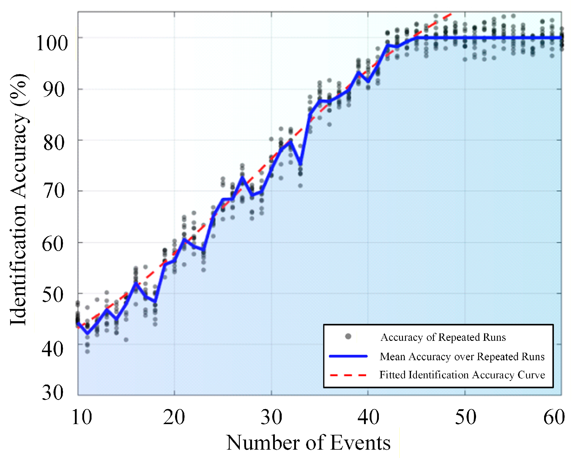
4.2.5. Impact of the Number of Events per Customer on Identification Accuracy

Due to HPLC bandwidth limitations, not all detected events can be transmitted to the master station. To determine the minimum event requirement and assess event-selection strategies, only voltage events were considered because current events are relatively sparse. Within each upload window, eligible response-voltage events were retained using ascending-magnitude, descending-magnitude, or uniform random sampling without replacement. As discussed in Section 2.2, event-phase voltage responses are typically four to six times larger than non-event-phase responses. Thus, high-magnitude events mainly strengthen same-phase clustering in Stage 1, whereas lower-magnitude but above-threshold events retain more neutral-coupled cross-phase information for Stage 2. Accordingly, the three strategies emphasize same-phase evidence, cross-phase evidence, and a balance of both, respectively. Therefore, a conservative strategy is adopted in this study, in which events are selected in ascending order of magnitude to achieve better identification performance.

As shown in Figure 11, identification accuracy improves progressively with increasing event availability and reaches a stable plateau near 100% at approximately 45 voltage events per 15 min window. Beyond this point, additional events provide negligible improvement. Thus, approximately 45 valid voltage events per window are sufficient for reliable identification, providing a practical event-retention guideline under HPLC bandwidth constraints.

4.3. Identification Results and Analysis

4.3.1. Same-Phase Customer Clustering Results

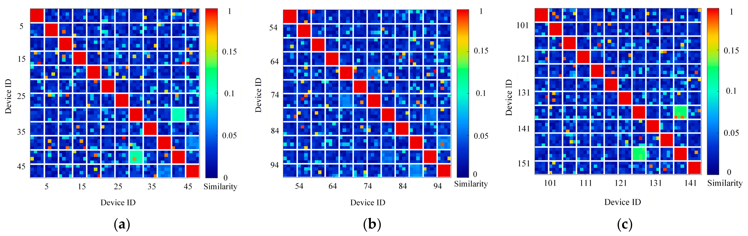
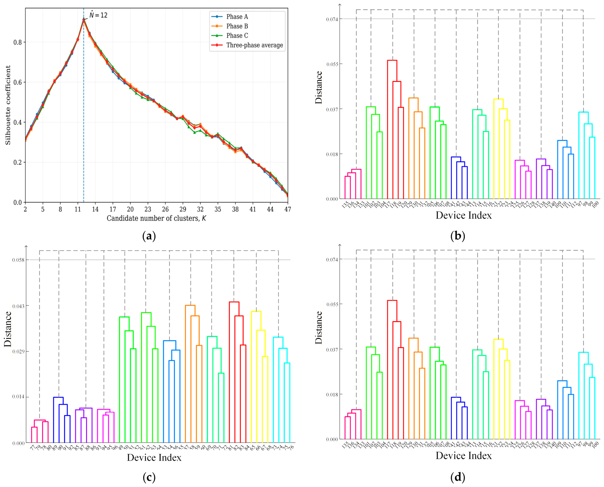
In the first stage, the similarities between the voltage event sequences of different customers are calculated based on dynamic response consistency. As shown in Figure 12, the clear diagonal block structure of the similarity matrix for customers of phase A, phase B, and phase C is presented. The candidate number of clusters was varied from 2 to 47. As shown in Figure 10a, the average silhouette coefficient of three phases reaches its global maximum at $K=\widehat{N}=12$, and this result is consistent with the manually verified number of electricity meter boxes. As shown in Figure 13b–d, through hierarchical clustering, 48 customers in each phase were accurately divided into 12 clusters, with 4 customers in each cluster, which is exactly consistent with the physical structure of the LVDN. The clustering accuracy in this stage reaches 100%, providing a basis for cross-phase matching.

4.3.2. Cross-Phase Cluster Combination Results

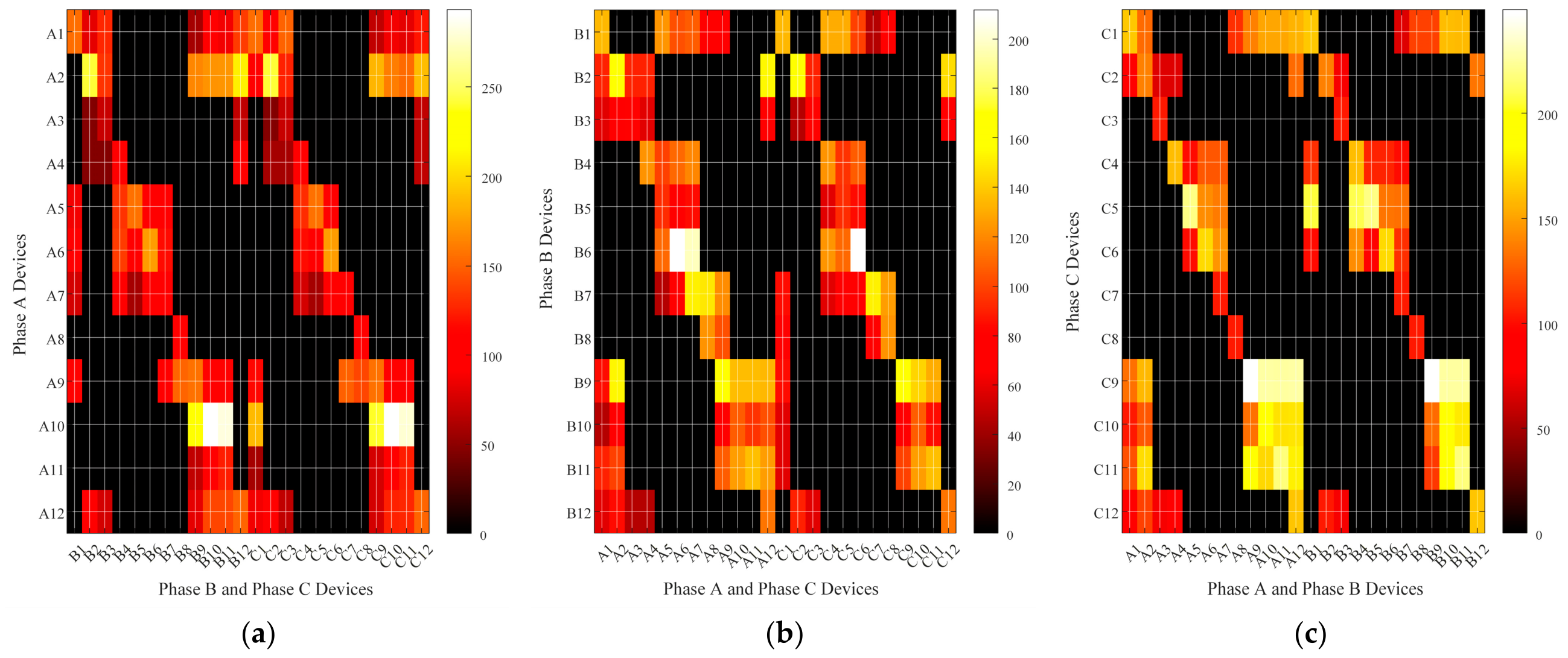
In the second stage, a multi-mode matching and multi-day voting strategy was adopted. As shown in Figure 14, the matching heatmaps of the three modes for a certain day is presented. In mode one, with phase A as the driving phase, the rows represent the 24 clusters of phases B and C, and the columns represent the 12 clusters of phase A. The bright cells reveal strong associations. For example, numerous synchronized events are observed between cluster A10 and clusters B10 and C10, indicating that they belong to the same meter box.

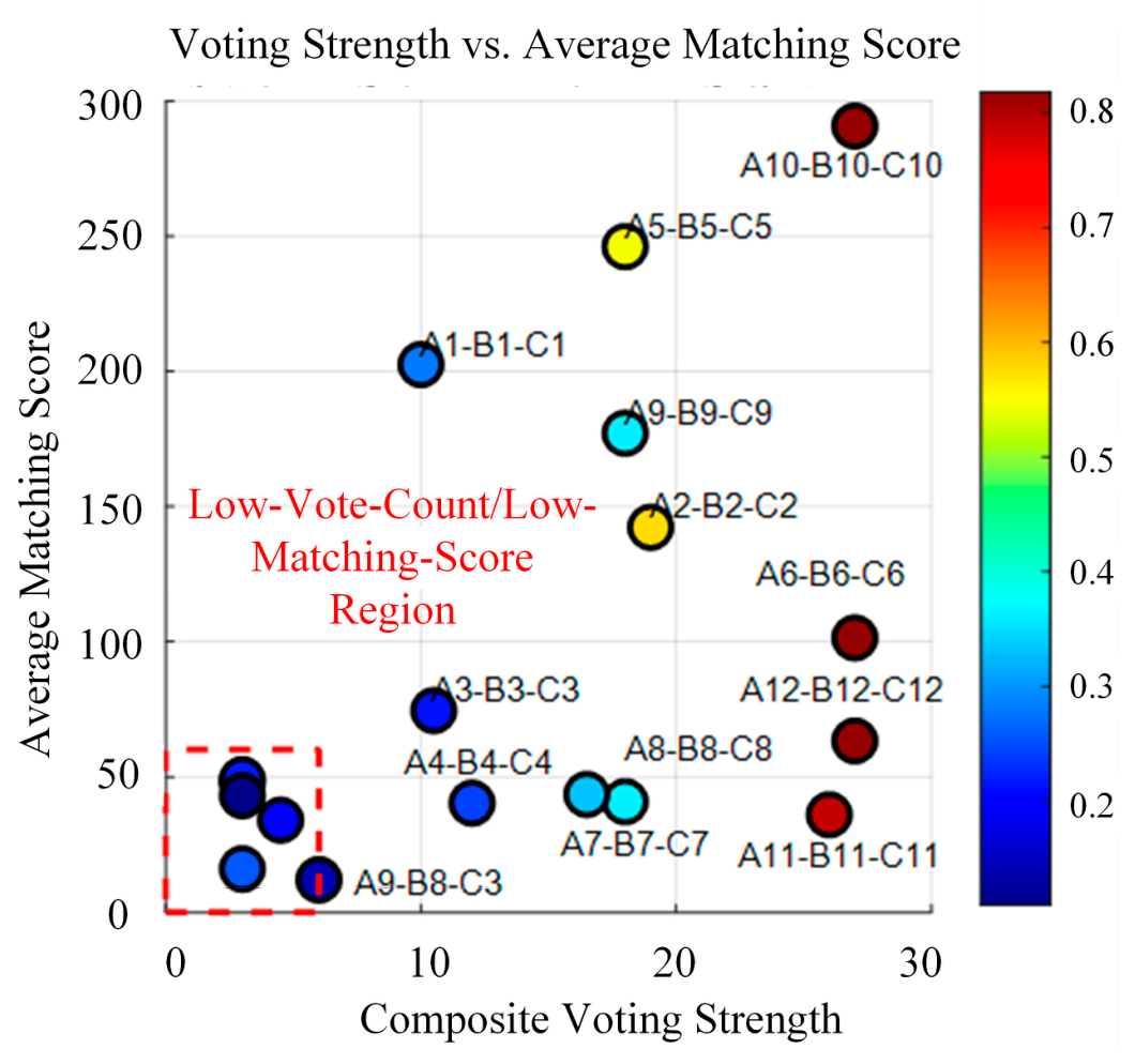
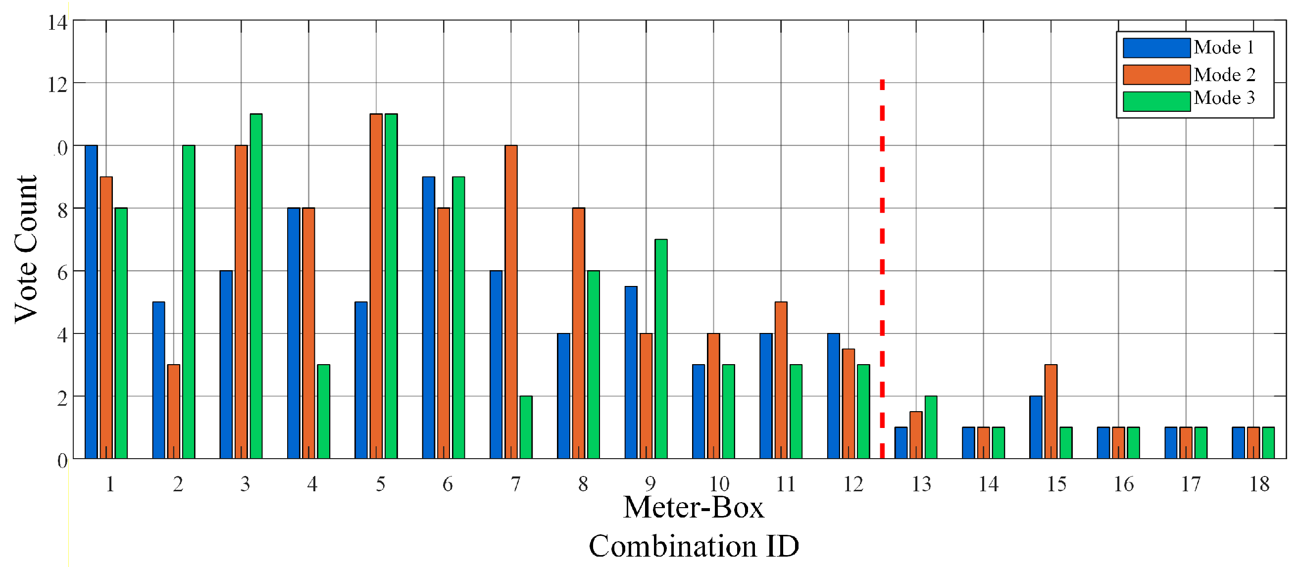
After accumulating votes over 10 days, the vote counts of all three-phase cluster combinations are shown in Figure A2 of Appendix A. There is a significant difference between the high-vote and low-vote combinations. Figure 15 further reveals a significant positive correlation between the voting intensity and the average matching degree, validating the high confidence of the high-vote combinations.

Finally, using the optimal assignment strategy, the system made decisions in descending order of vote count while ensuring that each cluster was uniquely assigned. Twelve conflict-free meter box combinations were obtained, as listed in

Table 2. Voting results for meter box combinations.

Meter Box	Phase A Group	Phase B Group	Phase C Group	Vote Count
Meter Box1	10	10	10	27
Meter Box2	5	5	5	18
Meter Box3	6	6	6	27
Meter Box4	2	2	2	19
Meter Box5	12	12	12	27
Meter Box6	11	11	11	26
Meter Box7	9	9	9	12
Meter Box8	8	8	8	12
Meter Box9	7	7	7	11
Meter Box10	1	1	1	10
Meter Box11	4	4	4	8
Meter Box12	3	3	3	7

. The reconstructed topology was compared with the topology records for the LVDN on a one-by-one basis. The proposed method achieves an identification accuracy of 100% for customer–meter box relationships.

4.4. Comparison of Identification Performance

All methods used the same 144 customers, verified phase labels and 10-day window; the 15 min inputs were aggregated from the same 20 ms records. For t-SNE+BIRCH, phase-wise Z-score normalization was followed by t-SNE (2 dimensions, perplexity 30, PCA initialization, automatic learning rate, and 1000 iterations) and BIRCH (threshold 0.50 and branching factor 50). Twenty runs with seeds 0–19 were averaged. For constrained K-medoids, Euclidean distance, PAM updates, silhouette-based preliminary cluster selection, and address-based must-link constraints were used. Twenty constraint-aware random initializations were performed, with a 300-iteration limit, and the minimum-dissimilarity solution was retained. Only this baseline used the address information required by its formulation. All settings were fixed without ground-truth labels; the proposed method is deterministic and was run once.

A comparison based on data from an actual LVDN in Nanjing shows that the proposed method achieves an accuracy of 100% for a test scenario containing 144 customers and 12 m boxes, with a normalized mutual information (NMI) value of 1. NMI is an important metric for measuring the consistency between the clustering results and the true labels [33]. The range of values is from 0 to 1, and a higher value indicates better clustering quality.

The comparative experiment in Table 3 shows that the performance improvement of the conventional method remains very limited, even when the sampling interval is reduced from 15 min to 0.02 s. This indicates that the traditional methods based on steady-state voltage similarity are inherently limited by the insufficient discrimination of steady-state features among customers with short electrical distances. Simply increasing the sampling frequency cannot overcome this limitation.

Table 3. Comparison of customer–meter-box identification performance across methods and sampling intervals.

Method	Sampling Frequency	Identification Accuracy (%)	NMI
t-SNE+BIRCH	0.02 s	77.4	0.79
t-SNE+BIRCH	15 min	75.2	0.77
K-medoids	0.02 s	85.4	0.86
K-medoids	15 min	81.2	0.83
Proposed Method	0.02 s	100	1.00

Table 3. Comparison of customer–meter-box identification performance across methods and sampling intervals.

Method	Sampling Frequency	Identification Accuracy (%)	NMI
t-SNE+BIRCH	0.02 s	77.4	0.79
t-SNE+BIRCH	15 min	75.2	0.77
K-medoids	0.02 s	85.4	0.86
K-medoids	15 min	81.2	0.83
Proposed Method	0.02 s	100	1.00

4.5. Robustness Analysis Under Different Operating Conditions

To evaluate the robustness of the proposed method under different operating conditions, a series of experimental scenarios were constructed using the OpenDSS simulation platform based on the three-phase four-wire low-voltage distribution network shown in Figure A1 of the Appendix. Ten days of actual customer load data collected during spring were used for testing, corresponding to the voting horizon, with a sampling interval of 0.02 s. In each test, the load profiles of individual customers at multiple time instants were assigned to the corresponding customer nodes in the test system. Twenty load-switching events were introduced at each customer node on phase A, with half corresponding to air-conditioning loads and the other half to electric-heating loads. Time-series power-flow calculations were then performed sequentially to obtain the current and voltage values of the remaining nodes before and after each switching event at a given customer node. Finally, the transient voltage and current events were extracted using the voltage and current thresholds determined from the sensitivity analysis described above.

4.5.1. Robustness Analysis with Different Customer Scales

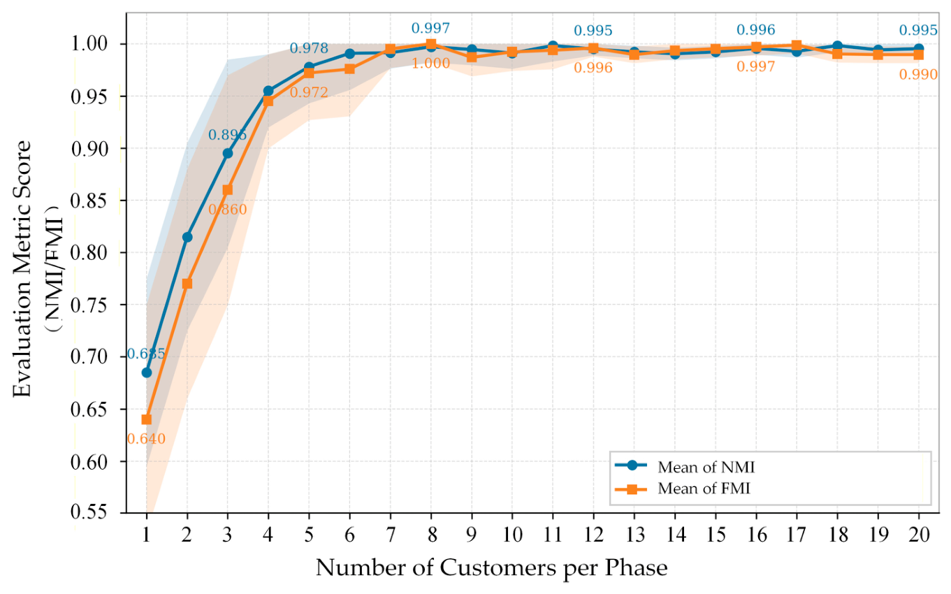
To evaluate the identification performance of the proposed method for different customer scales, the number of customers per phase in each meter box was gradually increased from 1 to 20, corresponding to an increase in the total number of customers from 18 to 360. The number of meter boxes was fixed at six and provided to the clustering stage in this experiment to isolate the effect of customer scale from the uncertainty in meter-box-count estimation.

Each experimental scenario was repeated 20 times. As shown in Figure 16, with the number of meter boxes known, the identification performance improves as the number of customers per phase in each meter box increases and tends to stabilize once the number reaches approximately 4–5 customers.

4.5.2. Robustness Analysis with Different Numbers of Meter Boxes

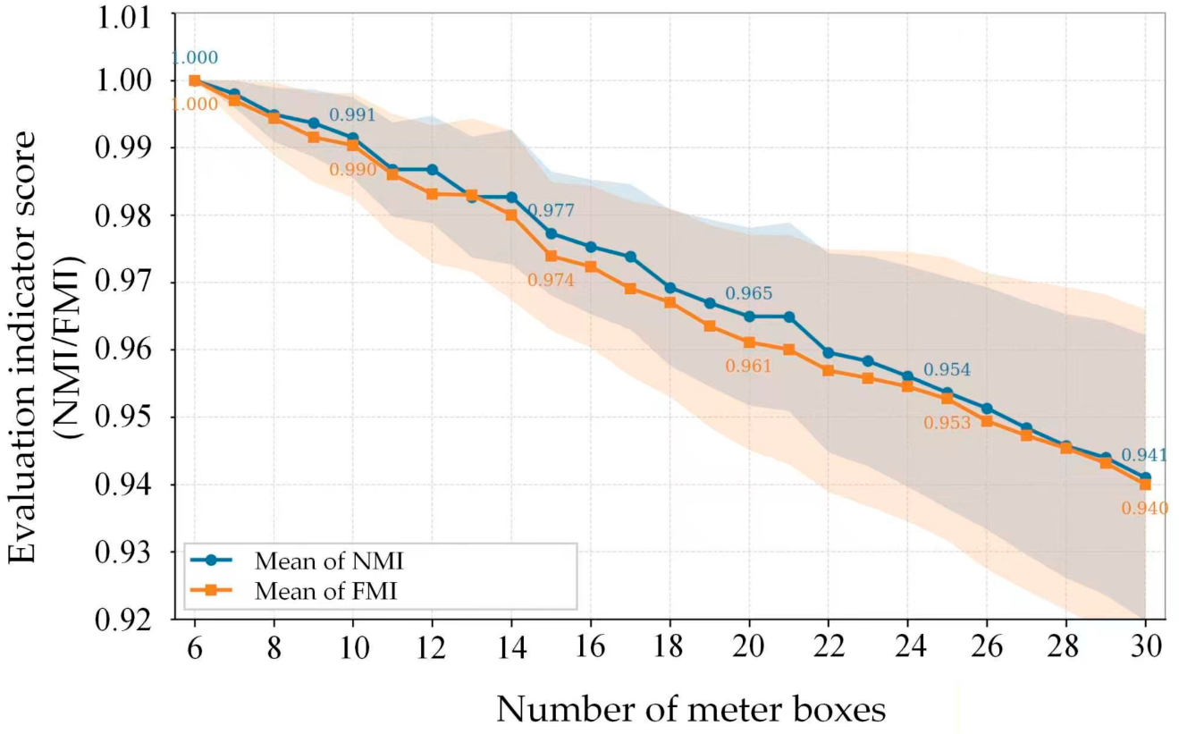
To assess the applicability and robustness of the proposed method across LVDN scales, OpenDSS scenarios containing 6–30 m boxes (108–540 customers) were constructed. Each meter box retained the same three-phase configuration with six customers per phase. Each scenario was repeated 20 times, and the mean NMI and FMI values with 95% confidence intervals are reported in Figure 17.

As the number of meter boxes increases, both metrics decline gradually. NMI and FMI remain above 0.98 for 6–14 m boxes, with a slightly faster decline beyond 16 boxes. Even at 30 m boxes, NMI and FMI remain at 0.941 and 0.940, respectively. These results demonstrate the robustness and scalability of the proposed method for customer–meter box identification in LVDNs of varying scales.

4.5.3. Robustness Analysis Under PV Integration Conditions

In OpenDSS, the PV array and grid-connected inverter were represented by a single PVSystem element. The model inputs comprised the inverter-rated apparent power (kVA), array peak power (kW), connection voltage (kV), and a maximum-power-point curve defined as a function of irradiance and temperature. To isolate the influence of photovoltaic active power injection on load switching characteristics, the same load curve, a sampling interval of 0.02 s, and a predefined event threshold are employed in all three scenarios.

The PV units were successively connected at nodes 1, 5, and 9 to form scenarios with one PV-connected nodes, as summarized in

Table 4. Influence of PV integration on the maximum voltage transient at node 13.

Scenario	PV Nodes	No-PV Max. ΔV (V)	With-PV Max. ΔV (V)	Mean Accuracy with-PV (%)
S1	1	−1.05	−1.06	100
S2	5	−2.28	−2.29	100
S3	9	−1.86	−1.88	100

. For each scenario, the same phase-A load-switching event was applied, and the maximum RMS-voltage change at the representative customer node 13 was compared with the no-PV baseline.

As shown in Table 4, although the pre-event operating voltage is shifted by local PV injection, the abrupt voltage change caused by the load-switching event remains nearly unchanged. Therefore, increasing the number of PV-connected nodes from one to three does not materially weaken the transient signature used by the proposed customer–meter-box identification method with the tested settings.

4.5.4. Robustness Analysis Under Statistical Variability Conditions

To assess the impact of different noise levels on the performance of this method, the following noise simulation experiments were conducted. Firstly, Gaussian white noise with a standard deviation ranging from 0% to 0.013% of the nominal voltage was added to the voltage measurement values of all user nodes (Table 5), with a step size of 0.003%. A total of nine noise scenarios were generated. For each scenario, the accuracy of customer–meter relationship identification was evaluated separately.

Table 5. Analysis of voltage noise sensitivity.

Added Noise σ (%)	Mean Accuracy (%)
0	100.0
0.001	100.0
0.004	100.0
0.007	100.0
0.01	100.0
0.013	99.4

Table 5. Analysis of voltage noise sensitivity.

Added Noise σ (%)	Mean Accuracy (%)
0	100.0
0.001	100.0
0.004	100.0
0.007	100.0
0.01	100.0
0.013	99.4

In practice, the voltage measurement error limits of class 0.2 S and class 0.5 S smart meters are 0.2% and 0.5% of the nominal voltage, corresponding to approximately 0.44 V and 1.1 V, respectively. Moreover, the nonsystematic measurement error is generally much smaller than the allowable systematic error limit of the meter. Based on engineering experience, the nonsystematic component is typically less than one-fifth of the total measurement error. Accordingly, using the more conservative error limit of a class 0.5 S meter and the $3\sigma$ criterion, the standard deviation $\sigma$ of the nonsystematic measurement error is estimated to be below approximately 0.07 V($\sigma =0.01\%$). This value is within the noise range over which the proposed method maintains stable identification performance, indicating that voltage measurement noise from smart meters of typical accuracy classes is unlikely to significantly affect the identification accuracy of the proposed method under normal operating conditions.

5. Conclusions

Accurately identifying the customer–meter box relationships identification with short electrical distances is the core challenge in the topology identification of LVDNs. The traditional methods based on steady-state voltage similarity are limited in effectiveness because of their insufficient discrimination. To overcome this limitation, this paper proposed a two-stage method for identifying customer–meter box relationships in low-voltage distribution networks, where short electrical distances make steady-state voltage profiles insufficiently discriminative. In the first stage, same-phase customers are clustered according to the similarity of their voltage-event sequences, and the number of meter boxes is estimated using a three-phase average silhouette criterion. In the second stage, cross-phase voltage responses caused by load-switching events are used to combine the single-phase clusters through event matching, multi-day voting, and a vote-priority assignment strategy, thereby reconstructing the complete customer–meter box topology.

A ten-day validation was conducted using both an actual residential LVDN in Nanjing comprising 144 customers and 12 m boxes and a series of low-voltage distribution network scenarios constructed using the OpenDSS simulation platform. The field case achieved an identification accuracy of 100%. The simulation results further show that variations in event count, customer scale, meter-box scale, voltage-fluctuation noise, and PV integration have only a limited impact on the identification performance of the proposed method. This validates the significant advantage of dynamic response features in identifying the meter box assignments of customers that are electrically close to one another, providing a new technical approach for subsequent accurate topology identification of LVDNs.

However, the reported performance may be affected by insufficient or overlapping switching events, timestamp and phase-label errors, missing measurements, lower sampling frequencies, and operating conditions that differ substantially from the assumptions used in the response model. Future work will therefore evaluate the method on more diverse low-voltage networks and further investigate its robustness under asynchronous measurement conditions, sparse events, distributed generation, electric-vehicle charging, and lower-frequency AMI configurations.

References

1. Nie, Z.; Han, Y.; Zhang, J.; Dai, R.; Yu, H.; Luo, J.; Chen, Y. Incoming Line Phase Identification of the Meter Box Bus of Low Voltage Distribution Network Using Circuit Terminal Unit. In Proceedings of the 2020 IEEE 4th Conference on Energy Internet and Energy System Integration (EI2), Wuhan, China, 30 October–1 November 2020; pp. 4184–4190. [Google Scholar] [CrossRef] [Scilit]
2. Yang, Z.; Shen, Y.; Yang, F.; Lei, Y.; Su, L.; Yan, F. Topology Identification Method of Low Voltage Distribution Network Based on Data Association Analysis. In Proceedings of the 2020 5th Asia Conference on Power and Electrical Engineering (ACPEE), Chengdu, China, 4–7 June 2020; pp. 2226–2230. [Google Scholar] [CrossRef] [Scilit]
3. Short, T.A. Advanced Metering for Phase Identification, Transformer Identification, and Secondary Modeling. IEEE Trans. Smart Grid 2013, 4, 651–658. [Google Scholar] [CrossRef] [Scilit]
4. Guo, X.; Xu, C.; Ming, Z.; Meng, B.; Yang, S.; Xu, L.; Zhu, Y. User–Feeder Topology Identification in Low-Voltage Residential Power Networks: A Clustering Fusion Approach. Energies 2025, 18, 4908. [Google Scholar] [CrossRef] [Scilit]
5. Ni, Q.; Jiang, H. Topology Identification of Low-Voltage Distribution Network Based on Deep Convolutional Time-Series Clustering. Energies 2023, 16, 4274. [Google Scholar] [CrossRef] [Scilit]
6. Duan, Y.; Liu, Z.; Liu, Y.; Li, Y. Signal Injection-Based Topology Identification for Low-Voltage Distribution Networks Considering Missing Data. Energies 2024, 17, 2060. [Google Scholar] [CrossRef] [Scilit]
7. Zhang, M.; Luan, W.; Guo, S.; Wang, P. Topology Identification Method of Distribution Network Based on Smart Meter Measurements. In Proceedings of the 2018 China International Conference on Electricity Distribution (CICED), Tianjin, China, 17–19 September 2018; pp. 372–376. [Google Scholar] [CrossRef] [Scilit]
8. Pappu, S.J.; Bhatt, N.; Pasumarthy, R.; Rajeswaran, A. Identifying Topology of Low Voltage Distribution Networks Based on Smart Meter Data. IEEE Trans. Smart Grid 2018, 9, 5113–5122. [Google Scholar] [CrossRef] [Scilit]
9. Zhao, J.; Xu, M.; Wang, X.; Zhu, J.; Xuan, Y.; Sun, Z. Data-Driven Based Low-Voltage Distribution System Transformer–Customer Relationship Identification. IEEE Trans. Power Deliv. 2022, 37, 2966–2977. [Google Scholar] [CrossRef] [Scilit]
10. Cook, E.; Saleem, M.B.; Weng, Y.; Abate, S.; Kelly-Pitou, K.; Grainger, B. Density-Based Clustering Algorithm for Associating Transformers with Smart Meters via GPS-AMI Data. Int. J. Electr. Power Energy Syst. 2022, 142, 108291. [Google Scholar] [CrossRef] [Scilit]
11. Al Khafaf, N.; Song, H.; McGrath, B.; Jalili, M. Identification of Low Voltage Distribution Transformer–Customer Connectivity Based on Unsupervised Learning. Energy Rep. 2023, 9, 72–79. [Google Scholar] [CrossRef] [Scilit]
12. Hu, H.; Zhao, J.; Bian, X.; Xuan, Y. Transformer–Customer Relationship Identification for Low-Voltage Distribution Networks Based on Joint Optimization of Voltage Silhouette Coefficient and Power Loss Coefficient. Electr. Power Syst. Res. 2023, 216, 109070. [Google Scholar] [CrossRef] [Scilit]
13. Lei, Y.; Yang, F.; Feng, Y.; Hu, W.; Cheng, Y. Two-Stage Transformer–Customer Relationship Identification Strategy for Low-Voltage Distribution Grid Using Physics-Guided Graph Attention Network. Energies 2025, 18, 4380. [Google Scholar] [CrossRef] [Scilit]
14. Wang, W.; Yu, N.; Foggo, B.; Davis, J.; Li, J. Phase Identification in Electric Power Distribution Systems by Clustering of Smart Meter Data. In Proceedings of the 2016 15th IEEE International Conference on Machine Learning and Applications (ICMLA), Anaheim, CA, USA, 18–20 December 2016; pp. 259–265. [Google Scholar] [CrossRef] [Scilit]
15. Xu, M.; Li, R.; Li, F. Phase Identification with Incomplete Data. IEEE Trans. Smart Grid 2018, 9, 2777–2785. [Google Scholar] [CrossRef] [Scilit]
16. Tang, X.; Milanović, J.V. Phase Identification of LV Distribution Network with Smart Meter Data. In Proceedings of the 2018 IEEE Power & Energy Society General Meeting (PESGM), Portland, OR, USA, 5–10 August 2018; pp. 1–5. [Google Scholar] [CrossRef] [Scilit]
17. Brint, A.; Poursharif, G.; Black, M.; Marshall, M. Using Grouped Smart Meter Data in Phase Identification. Comput. Oper. Res. 2018, 96, 213–222. [Google Scholar] [CrossRef] [Scilit]
18. Lee, H.P.; Rehm, P.J.; Makdad, M.; Miller, E.; Lu, N. A Novel Power-Band Based Data Segmentation Method for Enhancing Meter Phase and Transformer–Meter Pairing Identification. IEEE Trans. Power Deliv. 2024, 39, 2327–2339. [Google Scholar] [CrossRef] [Scilit]
19. Li, H.; Liang, W.; Liang, Y.; Li, Z.; Wang, G. Topology Identification Method for Residential Areas in Low-Voltage Distribution Networks Based on Unsupervised Learning and Graph Theory. Electr. Power Syst. Res. 2023, 215, 108969. [Google Scholar] [CrossRef] [Scilit]
20. Zhu, Y.; Yang, X.; Yan, H. Data-Driven Identification of Household-Transformer Relationships in Power Distribution Networks Using Hausdorff Similarity Assessment. Front. Energy Res. 2023, 11, 1233827. [Google Scholar] [CrossRef] [Scilit]
21. Hong, H.; Jin, F.; Pang, Z.; Zhan, Z.; Wu, M.; Tang, Y.; Zhao, J.; Pan, X. Improved Topology Identification Method for Low-Voltage Distribution Networks by Combining Quadratic Programming and Clustering. In Proceedings of the 2023 13th International Conference on Power and Energy Systems (ICPES), Chengdu, China, 8–10 December 2023; pp. 155–160. [Google Scholar] [CrossRef] [Scilit]
22. Lian, Z.; Yao, L.; Liu, S.; Yu, Y.; Tang, X.; Yang, L.; Lin, Z. Phase and Meter Box Identification for Single-Phase Users Based on t-SNE Dimension Reduction and BIRCH Clustering. Autom. Electr. Power Syst. 2020, 44, 176–184. (In Chinese) [Google Scholar] [CrossRef]
23. Luo, J.; Zhang, J.; Chen, Y.; Yao, L.; Ma, L.; Yu, H. Identification of Low-Voltage User Meter Box Combined with Known Phase and Address Information. Autom. Electr. Power Syst. 2021, 45, 115–121. (In Chinese) [Google Scholar]
24. Xu, Y.; Lv, J.; Wang, J.; Ye, F.; Ye, S.; Ji, J. Identifying Topology of Distribution Substation in Power Internet of Things Using Dynamic Voltage Load Fluctuation Flow Analysis. PeerJ Comput. Sci. 2024, 10, e1688. [Google Scholar] [CrossRef] [Scilit] [PubMed]
25. Awad, H.; Bayoumi, E.H.E. Resilient Grid Architectures for High Renewable Penetration: Electrical Engineering Strategies for 2030 and Beyond. Technologies 2026, 14, 112. [Google Scholar] [CrossRef] [Scilit]
26. Awad, H.; Bayoumi, E.H.E. Next-Generation Smart Inverters: Bridging AI, Cybersecurity, and Policy Gaps for Sustainable Energy Transition. Technologies 2025, 13, 136. [Google Scholar] [CrossRef] [Scilit]
27. Soliman, H.M.; Saleem, A.; Bayoumi, E.H.E.; De Santis, M. Harmonic Distortion Reduction of Transformer-Less Grid-Connected Converters by Ellipsoidal-Based Robust Control. Energies 2023, 16, 1362. [Google Scholar] [CrossRef] [Scilit]
28. Kersting, W.H. Distribution System Modeling and Analysis, 4th ed.; CRC Press: Boca Raton, FL, USA, 2017; ISBN 978-1-4987-7213-6. [Google Scholar]
29. Mai, T.T.; Haque, A.N.M.M.; Vergara, P.P.; Nguyen, P.H.; Pemen, A.J.M. Adaptive Coordination of Sequential Droop Control for PV Inverters to Mitigate Voltage Rise in PV-Rich LV Distribution Networks. Electr. Power Syst. Res. 2021, 192, 106931. [Google Scholar] [CrossRef] [Scilit]
30. Genton, M.G. Classes of Kernels for Machine Learning: A Statistics Perspective. J. Mach. Learn. Res. 2001, 2, 299–312. [Google Scholar]
31. Ah-Pine, J. An Efficient and Effective Generic Agglomerative Hierarchical Clustering Approach. J. Mach. Learn. Res. 2018, 19, 1–43. [Google Scholar]
32. Lavastida, T.; Lu, K.; Moseley, B.; Wang, Y. Scaling Average-Linkage via Sparse Cluster Embeddings. In Proceedings of the 13th Asian Conference on Machine Learning, Virtual Conference, 17–19 November 2021; Volume 157, pp. 1429–1444. [Google Scholar]
33. Strehl, A.; Ghosh, J. Cluster Ensembles—A Knowledge Reuse Framework for Combining Multiple Partitions. J. Mach. Learn. Res. 2002, 3, 583–617. [Google Scholar]
Figure 1. Typical low-voltage distribution network topology.
Energies 19 04388 g001
Figure 2. Schematic diagram of dynamic response principle in three-phase four-wire system.
Energies 19 04388 g002
Figure 3. Variation in the three-phase voltage components with the neutral-point displacement angle.
Energies 19 04388 g003
Figure 4. Voltage responses at different meter box locations to load-switching events: (a) customer with the load-switching event; (b) customers connected to the same meter box; (c) customers connected to different meter boxes on the same branch; (d) customers connected to different meter boxes on different branches.
Energies 19 04388 g004
Figure 5. Flowchart of the meter box relationship identification method.
Energies 19 04388 g005
Figure 6. Statistical distribution of customer voltage fluctuations in 10 LVDNs in Nanjing.
Energies 19 04388 g006
Figure 7. Monte Carlo distribution of the neutral-conductor current required for an observable cross-phase response.
Energies 19 04388 g007
Figure 9. Joint selection of voting-confidence thresholds. (a) Normalized vote margins of correct and incorrect assignments after preliminary vote screening. (b) Automatic-assignment accuracy and acceptance rate versus C min . The dashed line indicates the selected threshold C min = 0.225 .
Energies 19 04388 g009
Figure 10. GH-VP assignment results for different voting horizons. Panels (ah) correspond to summer and spring, respectively, with horizons of 1, 3, 7, and 10 days.
Energies 19 04388 g010
Figure 11. Effect of the number of events within a 15 min window on customer–meter box relationship identification accuracy.
Energies 19 04388 g011
Figure 12. Affinity matrix for customers of phase A, B, and C: (a) phase A devices 1–48; (b) phase B devices 49–96; (c) phase C devices 97–144.
Energies 19 04388 g012
Figure 13. Three-phase hierarchical: (a) silhouette coefficient versus candidate cluster number in the controlled validation; (b) phase A hierarchical cluster dendrogram; (c) phase B hierarchical cluster dendrogram; (d) phase C hierarchical cluster dendrogram.
Energies 19 04388 g013
Figure 14. Matching heatmaps of three patterns in one day: (a) heatmap of phase A current matching phase B and phase C; (b) heatmap of phase B current matching phase A and phase C; (c) heatmap of phase C current matching phase A and phase B.
Energies 19 04388 g014
Figure 15. Relationship between voting intensity and average matching degree.
Energies 19 04388 g015
Figure 16. Model identification performance in different customer-scale scenarios.
Energies 19 04388 g016
Figure 17. Trends in NMI and FMI with an increasing number of meter boxes.
Energies 19 04388 g017