A Dual-Stream Network with Dynamic Graph Convolution and Attention-Based BiGRU for IGBT Open-Circuit Fault Diagnosis in T-NPC Three-Level Inverters

Abstract

Existing CNN, TCN, residual, and lightweight network methods have achieved good performance in IGBT open-circuit fault diagnosis, but they often overlook the non-Euclidean relationships among signals. To address this limitation, this paper proposes a parallel graph–temporal network for T-NPC three-level inverters. A shared CNN extracts compact features from the three-phase currents and voltages, while the Sinkhorn–Wasserstein distance constructs a sample-level weighted dynamic graph for GCN-based relationship extraction. In parallel, BiGRU with global attention captures temporal information. Unlike fixed or equally weighted graphs, the proposed method adapts signal connections to different fault conditions. Furthermore, simulation models are constructed in MATLAB/Simulink, and the T-NPC converter operation is emulated on a real-time simulator Starsim MT6060. The proposed dual-stream model classifies 21 fault states, achieving an average validation accuracy of 99.88%, while maintaining high accuracy under severe noise.

1. Introduction

The transition toward low-carbon electricity has accelerated the deployment of renewable energy technologies in modern power systems [1]. Among multilevel converter topologies, the T-type neutral-point-clamped (T-NPC) inverter can reduce conversion losses compared with the conventional NPC configuration [2]. However, failures of power semiconductor devices remain a major threat to converter reliability [3,4].

For discussion, existing open-circuit fault diagnosis methods can be grouped into model-driven, signal-based, and data-driven approaches [5]. Model-driven methods infer faults from residuals or parameters derived from converter models. Jlassi et al. proposed a robust observer-based method for jointly diagnosing IGBT and current sensor faults [6]. Luo et al. used a fast recursive algorithm (FRA) to estimate current model parameters and diagnose single- and double-switch open-circuit faults [7]. Zhang et al. constructed phase voltage vector residuals across modulation modes and designed an adaptive diagnostic threshold [8]. These methods require converter models, estimated parameters, residual definitions, or thresholds, whose robustness must be assessed under parameter variations and measurement noise [6,7,8].

Signal-based and conventional machine learning methods transform measured currents or voltages into diagnostic features before classification. Kou et al. combined Concordia-transformed current trajectories with a random forest classifier [9]. Chen and Zhang combined knowledge reduction with extreme learning machine sub-classifiers for multiple-switch faults [10]. Deep learning methods further reduce manual feature designs by learning representations from sequences or encoded signal images. Representative approaches include a temporal convolutional network [11], a grayscale image CNN-SVM [12], GASF with an improved AlexNet [13], recurrence plots with a CNN [14], and an improved deep residual network [15]. However, these approaches mainly represent inputs as regular sequences or images rather than sample-specific relational structures.

Recent studies have extended data-driven diagnosis toward lightweight deployment, robustness, and multisource fusion. Xie et al. developed the lightweight 1D-DSCNN-GMP model for online edge diagnosis [16]. Yan et al. proposed a multiscale shuffled CNN for three-level NPC inverters [17]. Yang et al. integrated multisource information through an adaptive CNN–Transformer architecture [18]. Xing et al. developed a multimodal deep residual filter network for multiple open-switch faults [19]. Other studies addressed diagnosis under low-quality data [20] and transferable, noise-tolerant diagnosis across multiple inverters [21]. These methods improve deployability or robustness, but they do not explicitly represent the six current and voltage variables as a sample-specific weighted graph.

Parallel and graph-based diagnostic architectures demonstrate the value of learning complementary representations. Dual-branch feature fusion has been applied to wind turbine structural diagnosis [22]. Temporal graph convolution has also been investigated for photovoltaic fault diagnosis [23]. Lag-aware spatiotemporal dynamic graph networks have been developed for autonomous underwater vehicles [24]. However, their signal structures and fault propagation mechanisms differ from the voltage–current coupling of T-NPC inverters. Consequently, their graph definitions cannot be transferred directly to this diagnostic task.

Graph convolutional networks (GCNs) provide a suitable framework for learning relationships between variables. Li et al. proposed a multi-receptive field GCN incorporating weighted graphs and higher order neighborhoods for machinery diagnosis [25]. Gao et al. applied a semi-supervised GCN to rotating machinery fault diagnosis [26]. Zhang et al. subsequently introduced dynamic edge weight updating to accommodate changing vibration features [27]. Xiao et al. combined CNN feature extraction with dynamic graph convolution for multimodal fault diagnosis [28]. These studies demonstrate the value of graph-based relational learning, but their graph definitions do not directly encode fault-dependent voltage–current relationships in T-NPC inverters.

To address this gap, this study proposes a parallel dual-stream network that combines Sinkhorn-weighted dynamic graph convolution with an attention-based bidirectional gated recurrent unit (BiGRU). The three-phase currents and voltages are represented as six graph nodes and encoded using a shared one-dimensional convolutional neural network (CNN). CNNs employ shared convolutional kernels to learn compact local representations from structured inputs [29]. The resulting node features are normalized as discrete distributions, and their pairwise differences are evaluated using entropy-regularized optimal transport. The Sinkhorn matrix scaling algorithm provides an efficient approximation of the corresponding Wasserstein distances [30,31,32], which are then converted into a sample-specific weighted adjacency matrix. Following the standard neighborhood aggregation formulation of graph convolutional networks (GCNs) [33], the graph branch extracts relational features among the signal nodes. In parallel, the gated recurrent unit (GRU) uses reset and update gates to model temporal dependencies [34], while bidirectional recurrent processing incorporates information from both preceding and subsequent time steps [35]. A global attention mechanism evaluates all BiGRU hidden states and assigns greater weights to diagnostically informative temporal segments [36]. Finally, the graph and temporal representations are fused to classify 21 operating states of the T-NPC inverter.

Although the individual CNN, GCN, GRU/BiGRU, Sinkhorn, Wasserstein distance, and global attention operations follow established formulations, their task-specific integration constitutes the principal methodological contribution of this study. Specifically, entropy-regularized optimal transport is employed to construct a sample-specific six-node weighted graph, while the parallel attention-based BiGRU branch provides a complementary temporal representation. Thus, the proposed method focuses on the coordinated extraction and fusion of relational and temporal fault features rather than reformulating the individual algorithms.

Accordingly, the main contributions of this study are threefold. First, a six-node weighted graph is constructed for each sample using shared waveform encoding and Sinkhorn–Wasserstein distances, allowing the graph weights to adapt to the characteristics of each input sample. Second, parallel GCN and attention-based BiGRU branches independently extract relational and temporal representations, avoiding sequential feature propagation between the two branches. Third, a nonlinear feature fusion module combines these complementary representations for the diagnosis of 21 T-NPC operating states. Simulation experiments are conducted to evaluate the diagnostic performance of the proposed method, while the HIL platform is used to reproduce fault operating conditions and acquire experimental voltage and current signals.

The remainder of this paper is organized as follows. Section 2 analyzes single- and dual-IGBT open-circuit faults in T-NPC converters. Section 3 describes data preprocessing, dynamic graph construction, relational and temporal feature extraction, and feature fusion. Section 4 presents simulation studies, parameter analyses, ablation experiments, noise tests, and model comparisons. Section 5 reports hardware-in-the-loop validation, and Section 6 concludes this paper.

2. Open-Circuit Fault Analysis in Three-Level T-NPC Converters

2.1. Single-IGBT Open-Circuit Fault Analysis

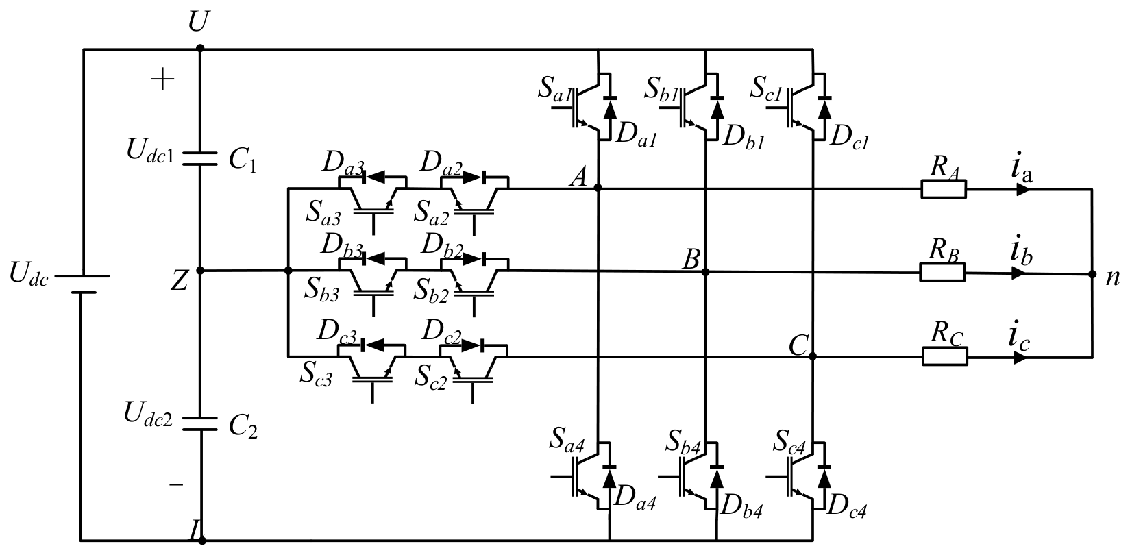
The ${\mathrm{T}}^2$3L topology is shown in Figure 1. The upper and lower bridge arms consist of two switch transistors ($S_{x1}$ and $S_{x2}$, x = a, b and c) and two internal switch transistors ($S_{x3}$ and $S_{x4}$). The series-connected DC coupling capacitors provide three voltage levels for each bridge: U_dc1, 0 and U_dc2.

Table 1. Phase current characteristics of single-IGBT open-circuit fault in phase-A.

Fault IGBT	Current Direction	Current Path	Change of State
$S_{a1}$	ia > 0	$S_{a1}\to D_{a2},S_{a3}$	$P\to O$
	ia < 0	$D_{a1}$	$-$
$S_{a2}$	ia > 0	$D_{a2},S_{a3}$	$-$
	ia < 0	$S_{a2},D_{a3}\to D_{a1}$	$O\to P$
$S_{a3}$	ia > 0	$S_{a3},D_{a2}\to D_{a4}$	$O\to N$
	ia < 0	$S_{a2},D_{a3}$	$-$
$S_{a4}$	ia > 0	$D_{a4}$	$-$
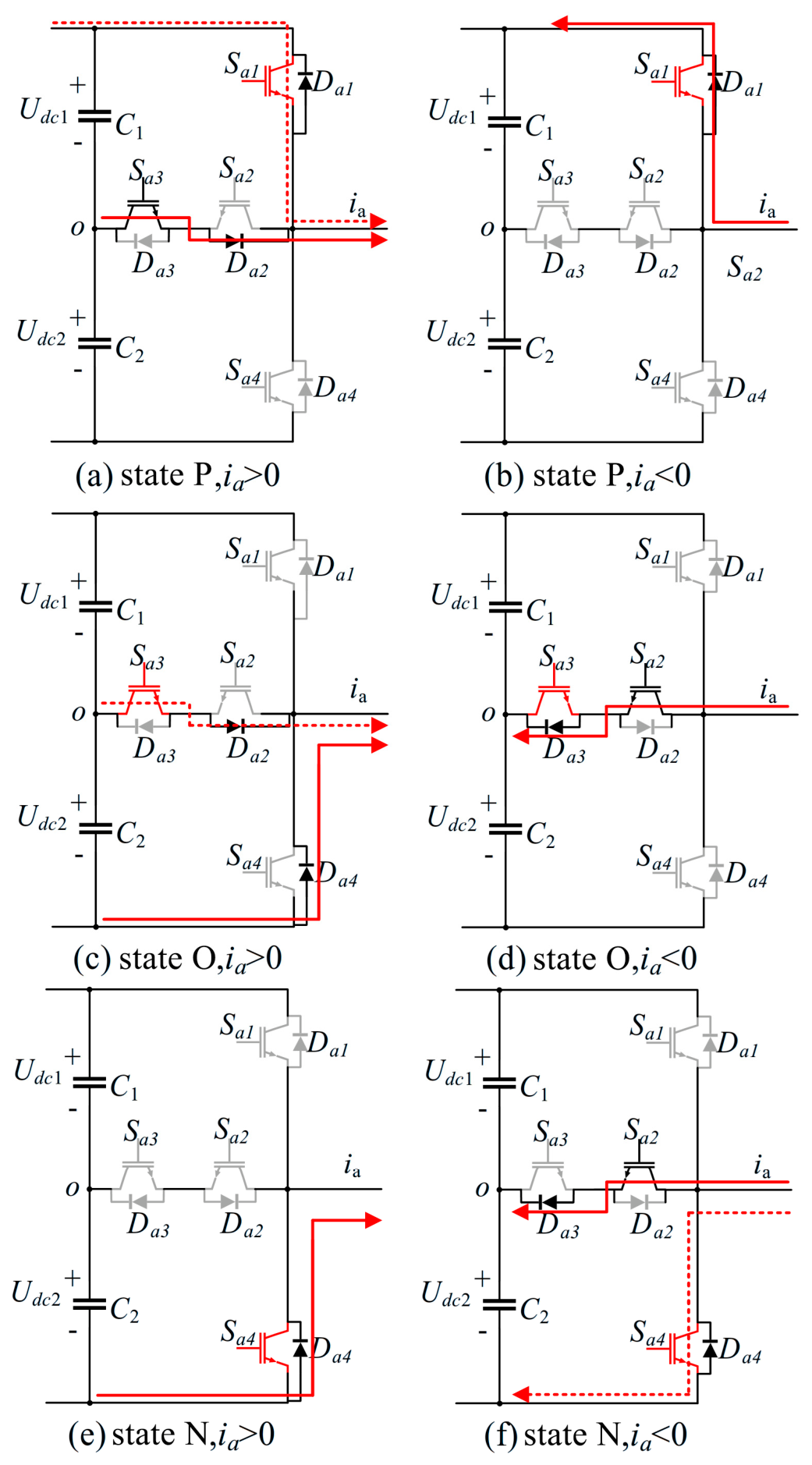
	ia < 0	$S_{a4}\to S_{a2},D_{a3}$	$N\to O$

illustrates the phase-A current paths under single-IGBT open-circuit faults. Under the S_a1 fault, the positive current cannot follow the state P path through S_a1; instead, it is redirected through S_a3 and D_a1, changing the output to state O and distorting the positive half-cycle, the current conduction paths before and after the switch fault. For i_a < 0, the current continues through D_a1, leaving state P and the negative half-cycle unaffected. Under an S_a3 fault, the positive current is diverted from S_a3 to D_a4. This changes the output from state O to N and distorts the positive half-cycle. For i_a < 0, conduction through S_a2 is maintained, so state O and the negative half-cycle remain unchanged. Open-circuit faults in other IGBTs can be analyzed in the same way. And the current paths are as shown in Figure 2. As shown in the Figure 2, the red switch symbols denote switches affected by open-circuit faults. The solid red lines indicate the actual post-fault current paths, whereas the dashed red lines indicate the corresponding current paths under normal operating conditions. The arrows indicate the direction of current flow.

2.2. Dual-IGBT Open-Circuit Fault Analysis

For dual-IGBT open-circuit faults occurring in different phases, the admissible conduction paths of the two affected legs can first be enumerated separately using the corresponding single-switch fault rules in Table 1, conditional on the instantaneous phase current directions. This phase-wise analysis is used only to identify the locally available switching and freewheeling paths; it does not imply that the two faults are dynamically independent or that their waveform effects can be linearly superimposed. By referencing

Table 2. Phase current characteristics of dual-IGBT open-circuit fault in phase-A.

Fault IGBTs	Current Direction	Change of State
$S_{a1}{S}_{a2}$	ia > 0	$P\to O$
	ia < 0	$O\to P$
$S_{a1}{S}_{a3}$	ia > 0	P$\to$N
	ia < 0	-
$S_{a1}{S}_{a4}$	ia > 0	$P\to O$
	ia < 0	$N\to O$
$S_{a2}{S}_{a3}$	ia > 0	$O\to N$
	ia < 0	$O\to P$
$S_{a2}{S}_{a4}$	ia > 0	-
	ia < 0	$N\to P$
$S_{a3}{S}_{a4}$	ia > 0	$O\to N$
	ia < 0	$N\to O$

, the changes in current paths for each phase were sequentially analyzed, yielding the variations in two-phase output voltage and switch states. For dual-IGBT faults in the same phase, the changes in current flow direction caused by the two faults interact with each other. During the $S_{a1}$ open-circuit fault, if the current $i_a$ > 0, it flows $S_{a3}$ through and $D_{a2}$. If the $S_{a3}$ fault also occurs during this state, the current flows through $D_{a4}$, causing the A-phase output state to transition from P to N. During the $S_{a2}$ open-circuit fault, if current $i_a$ > 0, it flows through $S_{a3}$, $D_{a2}$. If the $S_{a3}$ fault also occurs during this state, the current flows through $D_{a4}$, causing the A-phase output state to change directly from O to N. During the $S_{a3}$ open-circuit fault, if current $i_a$ < 0, it flows through $S_{a2}$ and $D_{a3}$. If the $S_{a2}$ fault also occurs during this state, the current flows through $D_{a1}$, causing the A-phase output state to change from O to P. During the $S_{a4}$ open-circuit fault, if current $i_a$ < 0, the current flows through $S_{a2}$ and $D_{a3}$ after the fault. If $S_{a2}$ also fails at this point, the current flows through $D_{a1}$, and the A-phase output state directly changes from N to P.

Table 3. Fault conditions and labels.

Faulty IGBT	Fault Label	Faulty IGBT	Fault Label
$S_{a1}$	0	$S_{a2}$$S_{b3}$	12
$S_{a1}$$S_{a2}$	1	$S_{a2}$$S_{b4}$	13
$S_{a1}$$S_{a3}$	2	$S_{a3}$	14
$S_{a1}$$S_{a4}$	3	$S_{a3}$$S_{a4}$	15
$S_{a1}$$S_{b1}$	4	$S_{a3}$$S_{b3}$	16
$S_{a1}$$S_{b2}$	5	$S_{a3}$$S_{b4}$	17
$S_{a1}$$S_{b3}$	6	$S_{a4}$	18
$S_{a1}$$S_{b4}$	7	$S_{a4}$$S_{b4}$	19
$S_{a2}$	8	Normal	20
$S_{a2}$$S_{a3}$	9
$S_{a2}$$S_{a4}$	10
$S_{a2}$$S_{b2}$	11

shows the 21 fault states and their corresponding labels. In the present study, 21 operating condition classes were considered, including 20 selected open-circuit fault conditions and one healthy condition, as listed in Table 3. These classes correspond to the conditions included in the constructed dataset and do not exhaust all possible single- and double-switch open-circuit fault combinations in the three-phase T-NPC inverter. The current classifier was only trained on and evaluated these 21 classes. Future work will expand the dataset to include the remaining phase-B and phase-C faults and other double-switch fault combinations, thereby extending the diagnostic and fault localization capabilities of the proposed method.

3. The Proposed Open-Circuit Fault Diagnosis Method

3.1. Data Description

Experimental data were acquired through a TCP/IP link established between the HIL MT6060 platform and the host computer. In parallel, a T-type three-level inverter was implemented in MATLAB 2024b/Simulink to generate simulated fault data. Each record contained 1024 sampling points for each of six signals. These signals included the three-phase output currents $i_a$, $i_b$, and $i_c$ and phase voltages $V_{\mathit{AO}}$, $V_{\mathit{BO}}$, and $V_{\mathit{CO}}$. For each IGBT fault condition, 300 records were independently acquired, while the dc-link voltage was varied within ±5% of its value of 800 V, and stored as matrices. These records were obtained through separate acquisition operations. The independently acquired datasets were randomly divided into training, validation, and test subsets at a ratio of 70%/15%/15%.

All datasets were stored in matrix formats to facilitate subsequent training and validation of the fault diagnosis model, which can be represented as follows:

$$X^{\left(n\right)}={\left[{i_a}^{\left(n\right)} {i_b}^{\left(n\right)} {i_c}^{\left(n\right)} {V_{\mathit{AO}}}^{\left(n\right)} {V_{\mathit{BO}}}^{\left(n\right)} {V_{\mathit{CO}}}^{\left(n\right)}\right]}^T\in R^{6\times 1024}$$

(1)

Due to differences in busbar voltages, the amplitude ranges of the three-phase voltages and three-phase currents acquired from the circuit topology vary. If these values are directly input into the model, voltage signals with larger amplitudes may dominate the gradient calculations. Therefore, it is necessary to preprocess the three-phase current and three-phase voltage datasets to normalize them to the same amplitude range while preserving the characteristics of the fault waveforms. Consequently, this paper employs the Z-score method to standardize the datasets. The specific process is as follows: First, calculate the mean of channel c:

$${\mu }_c={\displaystyle \frac{1}{N_{\mathit{tr}}T}}{\sum }_{n\in D_{\mathit{tr}}}{\displaystyle {\sum }_{t=1}^T}{X}_{c,t}^{\left(n\right)}$$

(2)

Then calculate its standard deviation as follows:

$${\sigma }_c=\sqrt{{\displaystyle \frac{1}{N_{\mathit{tr}}T}}{\sum }_{nϵD_{\mathit{tr}}}{\displaystyle {\sum }_{t=1}^T}{\left(X_{c,t}^{\left(n\right)}-{\mu }_c\right)}^2}$$

(3)

The normalized signal obtained by applying the above equation is:

$${\stackrel{\mathrm{~}}{X}}_{c,t}^{\left(n\right)}={\displaystyle \frac{x_{c,t}^{\left(n\right)}-{\mu }_c}{{\sigma }_c+\epsilon }}$$

(4)

The index c identifies one of the six signal channels corresponding to the three-phase currents and phase voltages. The index t denotes the sampling position and ranges from 1 to T, where T = 1024. $D_{tr}$ represents the training set, whereas $N_{\mathit{tr}}$ specifies the total number of training samples. For channel c, ${\mu }_c \mathrm{and} {\sigma }_c$, denote the mean and standard deviation calculated from $D_{\mathit{tr}}$, respectively. A small positive constant ε is introduced to avoid division by zero during normalization. The normalized value of the nth sample at channel c and sampling position t is denoted by ${\stackrel{\mathrm{~}}{X}}_{c,t}^{\left(n\right)}$.

3.2. Spatial Feature Extract-Based Graph Convolutional Network Module

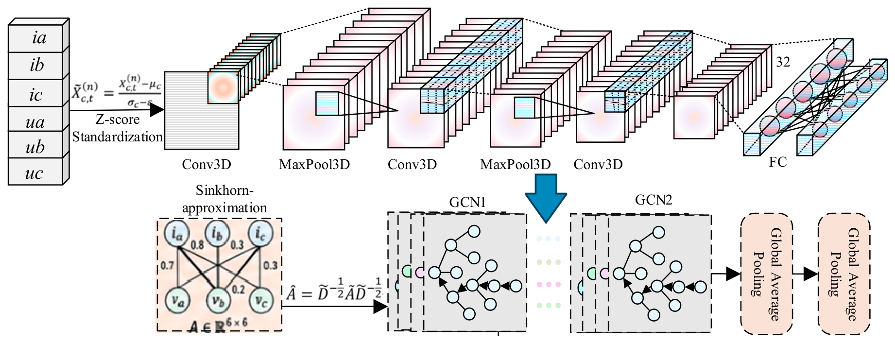
This paper constructs a six-node sample graph from three-phase currents and three-phase voltages, uses a shared CNN to compress node features, generates a weighted dynamic graph via the Sinkhorn–Wasserstein distance, and finally employs a GCN to extract features describing the relationships between current and voltage under fault conditions. Figure 3 shows the spatial feature extract network model.

3.2.1. CNN Construction

A two-layer CNN is used to encode the six electrical variable nodes. The CNN consists of two layers of convolutions, batch normalization, and ReLU activation functions, and converts each 1024 sampling points t waveform into 32-dimensional node features through adaptive average pooling and linear mapping, as shown in the following equation:

$$B_l\left(z\right)=\mathit{ReLU}\left[\mathit{BN}\right(W_l\times z+b_l\left)\right], l=1,2$$

(5)

$B_l$(·) represents the lth one-dimensional convolutional feature extraction block, and z denotes the input features to the current convolutional block. W_l and b_l are the kernel parameters and bias of the lth convolutional layer *: one-dimensional convolution operation. BN (·): batch normalization, used to stabilize the feature distribution and the training process. ReLU (·): nonlinear activation function, used to enhance the network’s feature representation capabilities. After passing through two convolution blocks, adaptive average pooling is used to reduce the temporal dimension, and a linear projection is applied to obtain the 32-dimensional features of the ith node:

$$H^{\left(0\right)}=\left[\begin{array}{c}{h}_{i_a}^{\left(0\right)}\\ h_{i_b}^{\left(0\right)}\\ h_{i_c}^{\left(0\right)}\\ h_{V_{\mathit{ao}}}^{\left(0\right)}\\ h_{V_{\mathit{bo}}}^{\left(0\right)}\\ h_{V_{\mathit{co}}}^{\left(0\right)}\end{array}\right]ϵR^{6\times 32}$$

(6)

The shared CNN down-samples the 1024 sampling points raw waveform using stride convolution and adaptive average pooling, compressing each electrical variable into 32-dimensional node features, thereby reducing the computational complexity of subsequent dynamic graph construction and graph convolution.

3.2.2. Sinkhorn-Weighted Dynamic Graph Model

The Sinkhorn algorithm approximates the pairwise Wasserstein distances d_ij among the six nodes in each sample. These distances measure differences between node feature distributions and are converted into edge weights to generate a sample-specific adjacency matrix and dynamic graph.

First, convert the node features into probability distributions.

$$p_{i,r}={\displaystyle \frac{\mathit{exp}\left(h_{i,r}^{\left(0\right)}\right)}{{\displaystyle {\sum }_{s=1}^F}\mathit{exp}\left(h_{i,s}^{\left(0\right)}\right)}}, F=32$$

(7)

$p_{i,r}$ is the probability of node i at the rth feature position, $h_{i,r}^{\left(0\right)}$ is the rth CNN feature of node i, and F = 32 is the feature dimension of the node. Accordingly, the resulting node distributions satisfy:

$$p_i,p_j\in {∆}^{F-1}, p_{i,r}\ge 0, {\displaystyle {\sum }_{r=1}^F}{p}_{i,r}=1$$

(8)

where ${∆}^{F-1}$ denotes the (F$-$1)-dimensional probability simplex.

The softmax-normalized vector is interpreted as a latent feature activation distribution rather than the physical amplitude distribution of the original waveform. Because the same CNN encoder is shared by all six current and voltage nodes, their feature vectors are represented in a common latent space. Softmax provides the non-negative unit mass marginals required by the Sinkhorn algorithm while preserving the relative activation strength of the learned features. Compared with constructing distributions directly from the 1024 sampling points time-domain amplitudes, the latent feature representation is more compact and less sensitive to absolute amplitude, phase displacement, operating condition variations, and measurement noise.

To define the ground cost, the F latent feature positions are assigned normalized support coordinates

$$u_r={\displaystyle \frac{r-1}{F-1}}, r=1,\dots ,F$$

(9)

Equivalently, each admissible transport plan must satisfy the marginal constraints

$${\displaystyle {\sum }_{s=1}^F}{P}_{\mathit{rs}}=p_{i,r},{\displaystyle {\sum }_{r=1}^F}{P}_{\mathit{rs}}=p_{j,s}$$

(10)

The Sinkhorn-approximated Wasserstein distance between node i and node j is defined as:

$$P_{\mathit{ij}}^{*}=\mathit{argmin}\left[〈P,C〉+\epsilon {\displaystyle {\sum }_{r=1}^F}{\displaystyle {\sum }_{s=1}^F}{P}_{\mathit{rs}}\left(\mathit{ln}{P}_{\mathit{rs}}-1\right)\right]$$

(11)

where C is the transport cost matrix, and ε > 0 is the entropy regularization coefficient, $〈P,C〉=\sum _{r,s}{P}_{\mathit{rs}}{C}_{\mathit{rs}}$

$$d_{\mathit{ij}}={\displaystyle {\sum }_{r=1}^F}{\displaystyle {\sum }_{s=1}^F}{P}_{\mathit{ij},\mathit{rs}}^{*}{C}_{\mathit{rs}}$$

(12)

where $P_{ij}^{*}$ represents the optimal transmission matrix between node i and node j; C is the transmission cost matrix between feature locations; and $P_{\mathit{ij},\mathit{rs}}^{*}$ denotes the quality of transmission from the rth feature location of node i to the sth feature location of node j. The smaller the value of $d_{\mathit{ij}}$, the more similar the fault feature distributions of the two nodes are. Since open-circuit faults in different switching devices affect each electrical variable differently, the adjacency matrix generated based on the Wasserstein distance can adaptively change according to the sample state.

Based on the Sinkhorn-approximated Wasserstein distance, the nearest nodes are selected from among the three current nodes and the three voltage nodes to define the dynamic weights:

$$A_{\mathit{ij}}=\left\{\begin{array}{c}exp\left(-{\displaystyle \frac{d_{\mathit{ij}}}{\tau }}\right)\\ 0, otherwise\end{array}\right.,j\in N_{\left(i\right)}$$

(13)

${\mathcal{N}}_{\left(i\right)}$ denotes the dynamic neighborhood set of node I, $A_{ij}$ denotes the dynamic edge weight between nodes i and j, and τ denotes the edge weight temperature coefficient.

The dynamic graph $g^{\left(n\right)}$ constructed using the above method contains information on the three-phase currents and three-phase voltages under different switching device failure conditions $v=\left\{i_a,i_b,i_c,v_{\mathit{AO}},v_{\mathit{BO}},v_{\mathit{CO}}\right\}$. $H^{\left(n,0\right)}ϵR^{6\times 32}$ and $A^{\left(n\right)}ϵR^{6\times 6}$ representing the connection relationships between pairs of nodes and are constructed via a CNN and the edge weight. Ultimately, this can be expressed by the following equation:

$$g^{\left(n\right)}=\left(V,H^{(n,0)},A^{\left(n\right)}\right)$$

(14)

3.2.3. Graphic Convolutional Network (GCN)

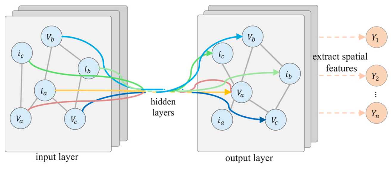
GCN treats each sampling location or current and voltage signal as a node and uses edges to describe the circuit topology and relationships between signals. Figure 4 shows a diagram of the GCN network structure. Figure 4. Schematic of the graph convolutional network. The colored solid arrows indicate the propagation and aggregation of node information through the hidden layers, with different colors used to distinguish the information-flow paths. The orange dashed arrows indicate the extraction of spatial features from the output-layer node representations to generat. All arrowheads indicate the direction of information flow.

In the proposed dual-stream branch structure, the GCN branch serves as an innovative topological feature extraction channel that complements the temporal or local features of the other branch, thereby enhancing the model’s ability to characterize complex fault patterns and improving the accuracy and robustness of open-circuit fault diagnosis in switching devices. The GCN processing procedure is as follows:

Once the adjacency matrix A is obtained, the self-loop is added as follows:

$$\widehat{A}=A+I$$

(15)

where I is the identity matrix; the inclusion of the self-loop indicates that, during graph convolution, each node retains its own information.

$${\widehat{D}}_{\mathrm{ii}}={\sum }_j{\stackrel{\mathrm{~}}{A}}_{\mathit{ij}}$$

(16)

Perform symmetric normalization on the adjacency matrix:

$$\widehat{A}={\stackrel{\mathrm{~}}{D}}^{-{\displaystyle \frac{1}{2}}}\stackrel{\mathrm{~}}{A}{\stackrel{\mathrm{~}}{D}}^{-{\displaystyle \frac{1}{2}}}$$

(17)

The first layer of the GCN is:

$$H^{\left(1\right)}=\mathit{Dropout}\left[\mathit{ReLU}\left(\mathit{BN}\left(\widehat{A}{H}^{\left(0\right)}{W}^{\left(0\right)}\right)\right)\right]H^{\left(1\right)}\in R^{6\times 64}$$

(18)

The second GCN layer is defined as:

$$H^{\left(2\right)}=\mathit{Dropout}\left[\mathit{ReLU}\left(\mathit{BN}\left(\widehat{A}{H}^{\left(1\right)}{W}^{\left(1\right)}\right)\right)\right]H^{\left(2\right)}\in R^{6\times 32}$$

(19)

The graph-level feature obtained through global average pooling is:

$$f_g=\mathit{GAP}\left(H^{\left(2\right)}\right)={\displaystyle \frac{1}{N}}{\displaystyle {\sum }_{i=1}^N}{h}_i^{\left(2\right)}$$

(20)

3.3. Temporal Feature Extraction Based on BiGRU with Global Attention

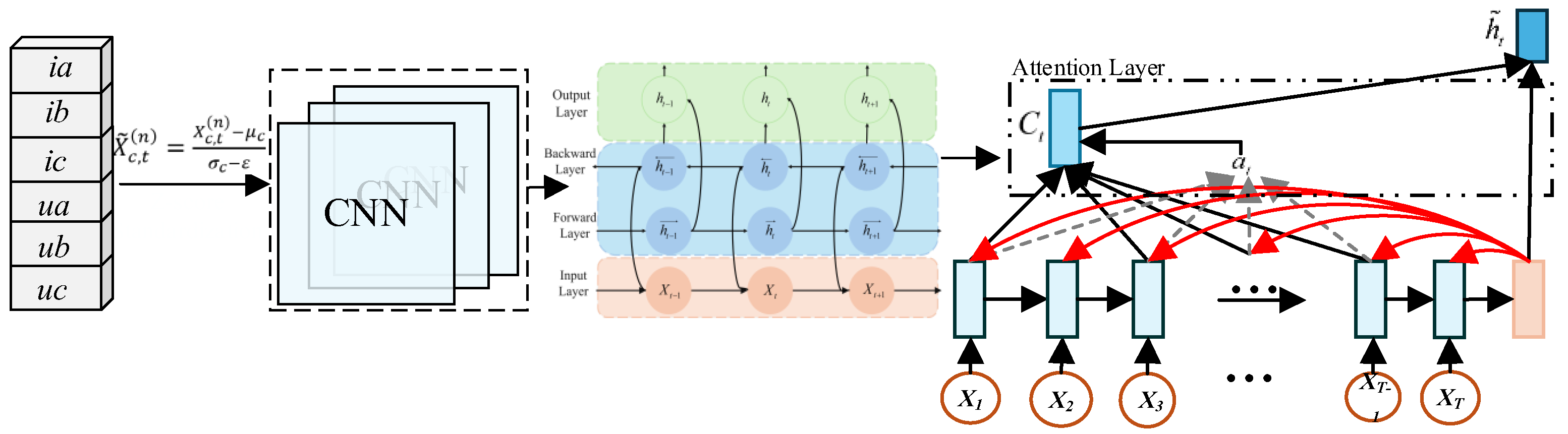
The time-series branch employs BiGRU to simultaneously capture the forward and backward dependencies of three-phase current and three-phase voltage signals, and combines a global attention mechanism to dynamically assess the importance of each time-series segment, thereby highlighting key features during fault events while suppressing noise and redundant information. Figure 5 shows the temporal feature extraction network model.

3.3.1. BiGRU Construction

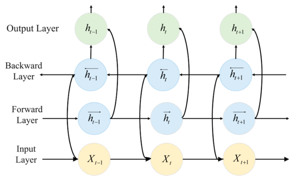
In order to address the vanishing gradient problem in the GRUs, they utilize two gates in the GRUs. Indeed, selecting information for the output is made by two vectors trained to preserve information from the past for a better classification. As shown in Figure 6, the structure of the BiGRU is:

$${\overrightarrow{h}}_t=GRU(x_t,{\overrightarrow{h}}_{t-1})$$

(21)

$${\overleftarrow{h}}_t=GRU(x_t,{\overleftarrow{h}}_{t-1})$$

(22)

$$h=W_{{\overrightarrow{h}}_t}{\overrightarrow{h}}_t+W_{{\overleftarrow{h}}_t}{\overleftarrow{h}}_t+b_t$$

(23)

Among these, GRU is a traditional GRU network computation process. $W_{{\overrightarrow{h}}_t}$ and ${\overrightarrow{h}}_t$ are the states and weights of the current forward hidden layer. $W_{{\overleftarrow{h}}_t}$ and ${\overleftarrow{h}}_t$ are the states and weights of the backward hidden layer at that time. $b_t$ is the offset of the hidden layer state at time t.

3.3.2. BiGRU Network with Optimized Global Attention

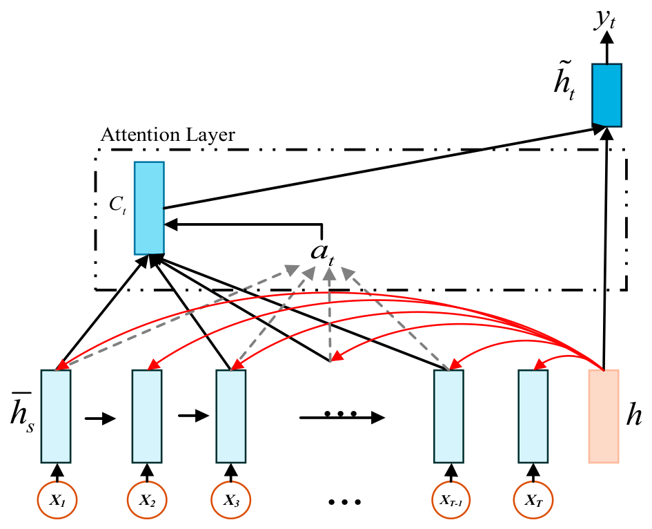
Global attention derives the context vector $c_t$ from all encoder hidden states. The current target-side state $h_t$ is compared with each source state ${\stackrel{\mathrm{-}}{h}}_s$, producing an alignment vector $a_t$, whose length equals the source sequence:

$$a_t\left(s\right)=\mathit{align}(h_t,{\stackrel{\mathrm{-}}{h}}_s)={\displaystyle \frac{\mathit{exp}\left(\mathit{score}\left(h_t,{\stackrel{\mathrm{-}}{h}}_s\right)\right)}{{\sum }_{s^{‘}}\mathit{exp}\left(\mathit{score}\left(\left(h_t,{\stackrel{\mathrm{-}}{h}}_{s^{‘}}\right)\right)\right)}}$$

(24)

At time step t, the model derives the variable-length alignment vector $a_t$ by matching $h_t$ with all source states ${\stackrel{\mathrm{-}}{h}}_s$. These weights combine the source states into the global context vector $c_t$, as illustrated in Figure 7. The colors distinguish the different feature representations, the black arrows indicate the direction of feature propagation, the red curved arrows represent the global-attention connections, and the gray dashed arrows labeled $a_t$ denote the corresponding attention weights.

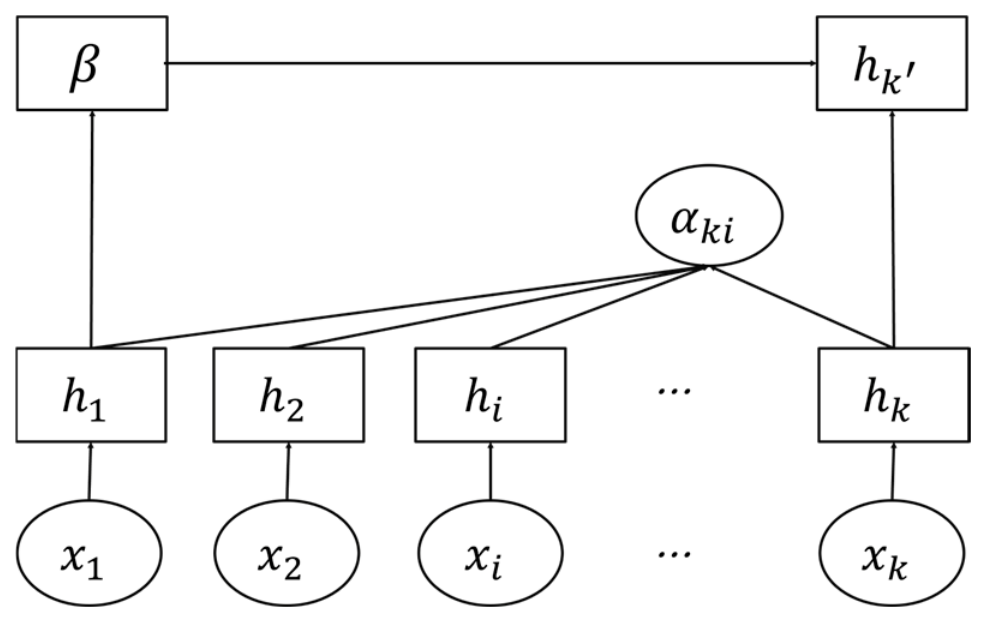
Global attention assigns an importance weight to each time step in the BiGRU output. It then aggregates the temporal features through weighted summation, allowing the model to emphasize fault-relevant segments while suppressing noisy or uninformative information. By focusing on the most informative temporal patterns, this mechanism can improve feature discrimination and potentially enhance model generalization. The structure of this attention process is illustrated in Figure 8.

Here, $x_1$, $x_2$, $x_i$, …, $x_k$ denote the input sequence, while $h_1$, $h_2$, $h_i$, …, $h_k$ are the corresponding BiGRU hidden states. Coefficient ${\alpha }_{\mathit{ki}}$ represents the attention assigned to the ith historical hidden state relative to the final hidden state; β denotes the overall hidden state weight, and $h_{k^{‘}}$ is the hidden state of the final output node. The global attention mechanism is mainly determined by ${\alpha }_{\mathit{ki}}$, which is calculated using Equations (25) and (26).

$${\alpha }_{ki}={\displaystyle \frac{\exp (e_{ki})}{{\displaystyle {\sum }_j^l\exp (e_{ki})}}}$$

(25)

$$e_{ki}=V\tanh (W{h}_k+U{h}_i)$$

(26)

where $e_{\mathit{ki}}$ denotes the energy score of the hidden state at position i, l is the input sequence length, and V and U are trainable weight matrices. Equations (27) and (28) define the semantic representation and output feature vectors used to obtain the global attention distribution:

$$\beta ={\displaystyle \sum _{i=1}^l{\alpha }_{ki}{h}_i}$$

(27)

$$h_{k^{\prime }}=H(\beta ,h_k,x_k)$$

(28)

3.3.3. Temporal Feature Output

The final forward and backward hidden states of BiGRU are concatenated to form a query vector. This query vector is used to compute correlations with all 64 time slices, generating a 64-element attention distribution. A weighted sum of all BiGRU outputs is then computed to obtain a global context vector.

$$c={\displaystyle {\sum }_{t=1}^T}{\alpha }_t{h}_t\in R^{B\times 96}$$

(29)

where ${\alpha }_t$ is the attention weight for the tth time slot, $h_t$ is the 96-dimensional BiGRU hidden state for the t-th time slot, and ${\alpha }_t{h}_t$ denotes the attention-weighted result for the tth time slot.

Concatenate the global context vector and the query vector:

$$f_{\mathit{pre}}^t=\left[c\parallel q\right]\in R^{B\times 192}$$

(30)

$f_{\mathit{pre}}^t$ represents the concatenated features before the temporal branch output mapping; c is the attention context vector; and q is the global query vector.

The final output features of the temporal branch are:

$$f_t=\mathit{Dropout}\left\{\mathit{ReLU}\left[\mathit{LN}\left(W_t{f}_{\mathit{pre}}^t+b_t\right)\right]\right\}$$

(31)

where $f_{\mathit{pre}}^t=\left[c\parallel q\right]\in R^{B\times 192}$ is obtained by concatenating the 96-dimensional attention context vector $\mathrm{c}$ and the 96-dimensional BiGRU query vector q. The context vector aggregates attention-weighted information from all time steps, whereas the query vector summarizes the bidirectional temporal dependencies of the complete sequence. The trainable matrix $W_t$ and bias $b_t$ project this representation into a 128-dimensional temporal feature space. Layer normalization stabilizes the feature distribution, ReLU introduces nonlinearity, and dropout reduces overfitting. The resulting temporal feature is subsequently fused with the graph branch feature for fault classification.

3.4. Dual Feature Stream Fusion Method

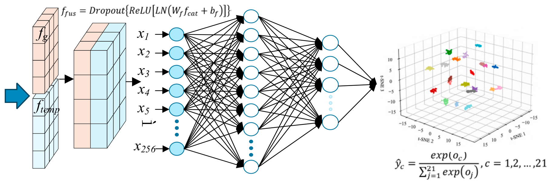
The graph convolutional branch captures fault-dependent coupling between the three-phase currents and voltages through information propagation over the dynamic graph. The temporal branch uses BiGRU and global attention to model bidirectional temporal dependencies and identify diagnostically important time segments. Figure 9 shows that the spatial and temporal feature fusion and classification. The orange and blue blocks represent the spatial features extracted by the GCN branch and the temporal features extracted by the temporal branch, respectively. The blue arrows indicate the direction of feature propagation, while the black lines denote the connections between adjacent fully connected layers. The light-blue circles represent neurons. In the t-SNE visualization, different colors denote the 21 operating-state categories.

The outputs of both branches are independently projected into a shared 128-dimensional feature space. They are then concatenated and nonlinearly fused to form the final fault representation. By exploiting the complementary spatial relations and temporal dynamics, the fused representation enables the identification of 21 operating states. The specific procedure is defined as follows:

The projection process for the integral branch and the temporal branch of the scroll is as follows:

$${\widehat{f}}_g=\mathit{ReLU}\left[\mathit{LN}\left(W_g^p{f}_g+b_g^p\right)\right]$$

(32)

$${\widehat{f}}_{\mathit{temp}}=\mathit{ReLU}\left[\mathit{LN}\left(W_{\mathit{temp}}^p{f}_{\mathit{temp}}+b_{\mathit{temp}}^p\right)\right]$$

(33)

After combining the integral branch and the time-series branch, the following equation is obtained:

$$f_{\mathit{fus}}=\mathit{Dropout}\left\{\mathit{ReLU}\left[\mathit{LN}\left(W_f{f}_{\mathit{cat}}+b_f\right)\right]\right\}$$

(34)

Finally, the fused features are fed into a fully connected classifier to obtain the classification results for the 21 fault states:

$$o=W_o{f}_{\mathit{fus}}+b_oϵR^{B\times 21}$$

(35)

where $o$ represents the 21-dimensional classification logits, $W_o$ is the classifier weight matrix, and $b_o$ is the classifier bias. The class scores are converted to predicted probabilities using the Softmax function:

$${\widehat{y}}_c={\displaystyle \frac{\mathit{exp}\left(o_c\right)}{{\displaystyle {\sum }_{j=1}^{21}}\mathit{exp}\left(o_j\right)}}, c=1,2,\dots ,21$$

(36)

The final diagnosis category is:

$$\widehat{c}=\mathit{argmax}{\widehat{y}}_c,cϵ\left\{1,\dots ,21\right\}$$

(37)

4. Simulation Verification

4.1. IGBT Open-Circuit Fault Characteristics Analysis

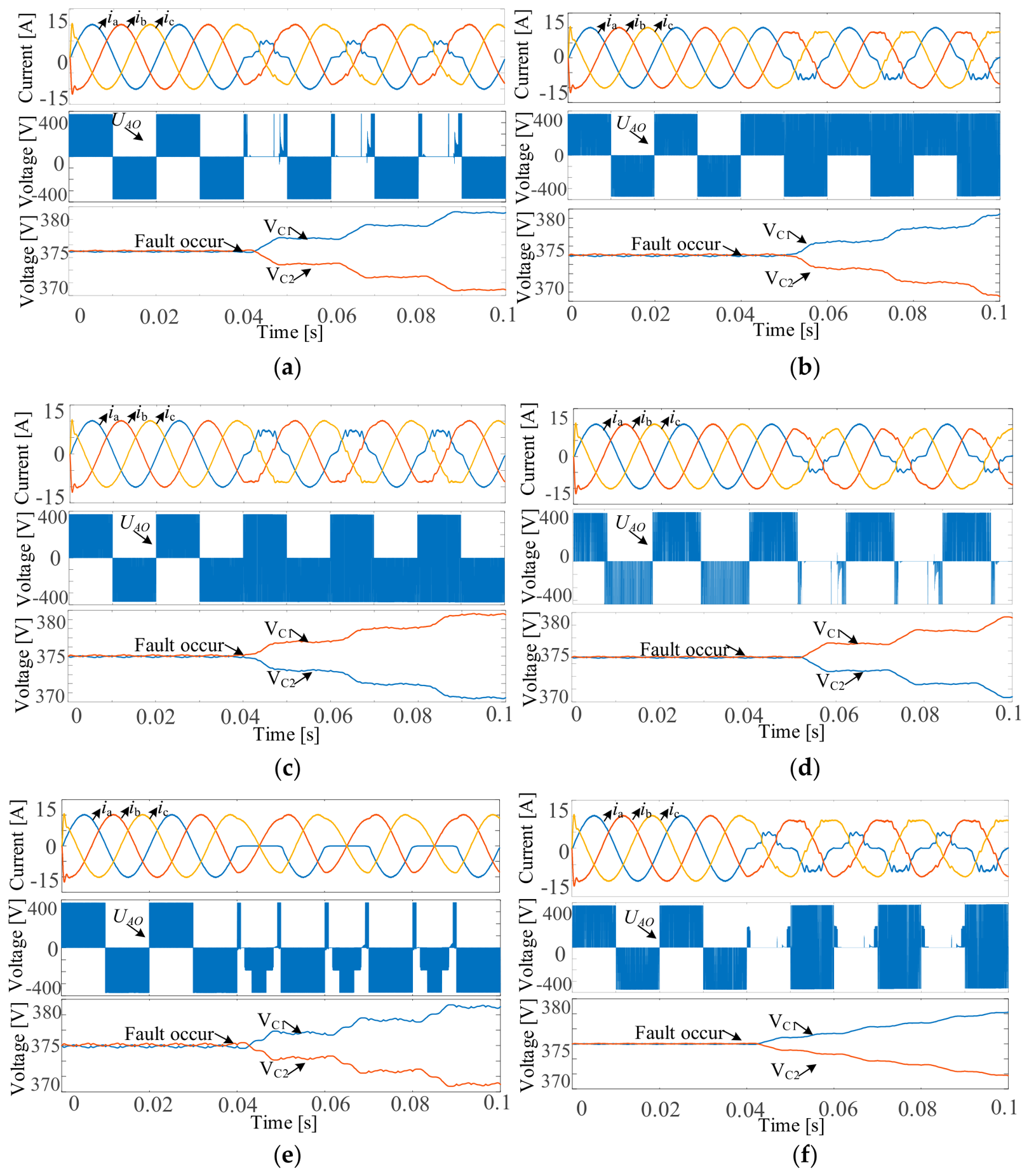
A MATLAB2024b/Simulink model configured with the parameters in

Table 4. Simulation parameters.

Notation	Parameters	Parameter Value
$U_{\mathit{dc}}$	DC side voltage	800 V
C1, C2	DC side capacitance	4000 µF
$f_s$	Switching frequency	20 kHz
$R$	Load resistance	30 Ω
$L_f$	Filter inductors	3 mH
$C_f$	Filter capacitor	8000 µF

was used to examine single- and dual-IGBT open-circuit faults in the T-type inverter. For phase-A, Figure 10 shows the three-phase currents i_a, i_b, and i_c, phase-A arm voltage U_AO, and dc-link capacitor voltages U_dc1 and U_dc2. Figure 10a–f correspond to faults in S_a1, S_a2, S_a3, S_a4, S_a1S_a2, and S_a1S_a3, respectively. These cases match those analyzed in Table 1 and Table 2.

4.2. IGBT Open-Circuit Fault Diagnosis Results

4.2.1. Training Procedure

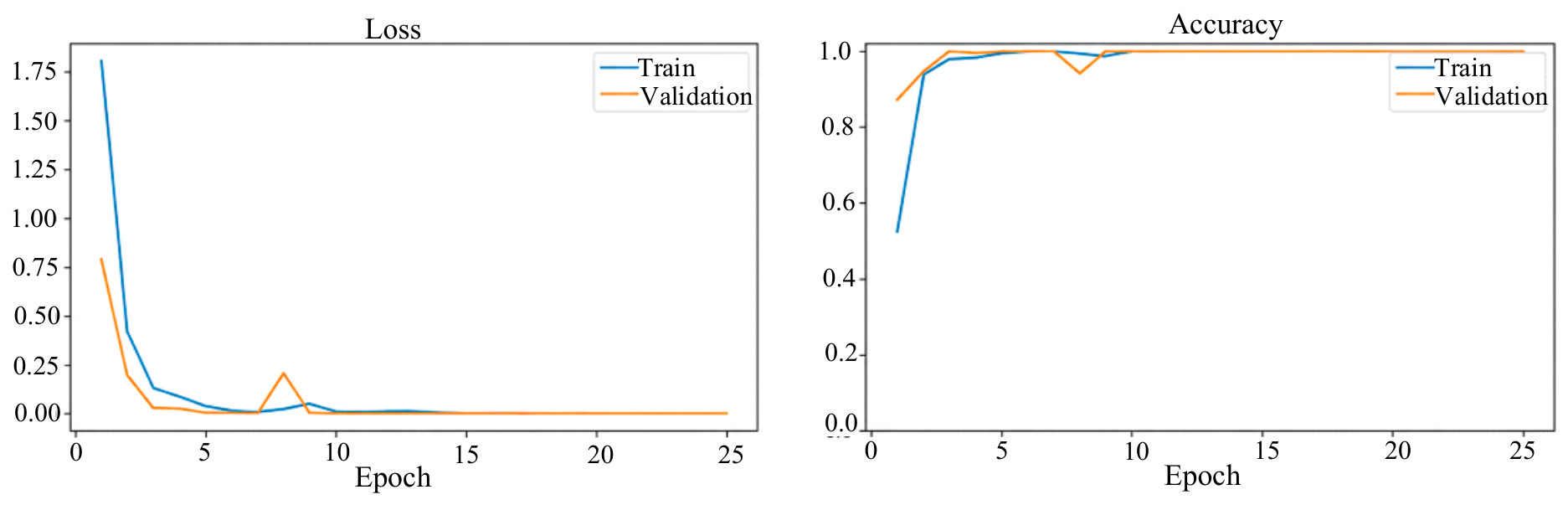
The training process parameter settings are shown in

Table 5. Experimental environment and training configuration parameters.

Parameters	Parameter Value
Processor	Intel Core i7-14900
Memory	16 GB RAM
GPU	NVIDIA GeForce GTX 5060
Data split	Training/validation/test = 70%/15%/15%
Learning rate	$1\times {10}^{-3}$
Weight decay	$1\times {10}^{-4}$
Batch size	64
Dropout rate	0.25

. The proposed model demonstrates stable convergence behavior during training. As illustrated in Figure 11, the loss curve decreases rapidly within the first 10 epochs and gradually converges. The accuracy curves for both the training and validation sets exhibit synchronous convergence, stabilizing after approximately 15 epochs with minimal fluctuation. This behavior suggests that the model effectively captures discriminative fault features from both the spatial and temporal domains. The final validation accuracy reaches 99.88%.

4.2.2. Selection of Entropy Regularization Parameters

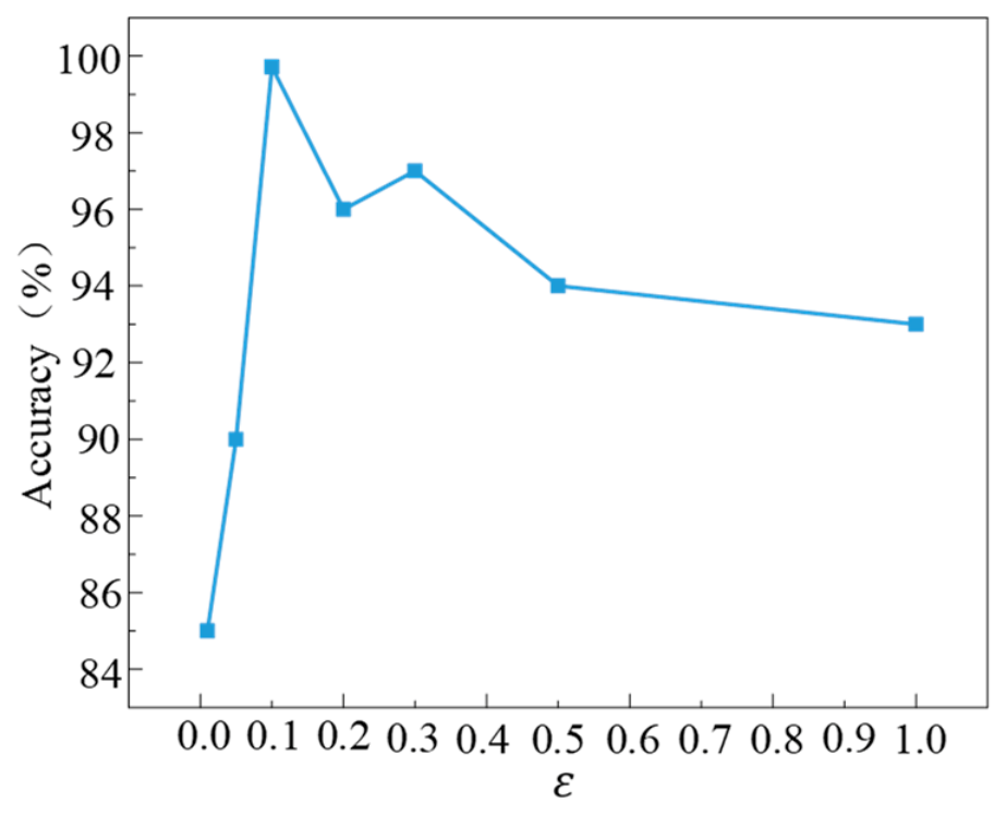
The entropy regularization parameter ε controls the trade-off between Wasserstein approximation accuracy and the discriminability of the resulting dynamic graphs. When ε was too small, the transport plan became sparse, convergence slowed, and the graphs became more sensitive to noise and DC-bus voltage fluctuations. When ε was too large, excessive smoothing reduced differences between node distances, producing similar graph structures and weakening fault class separability. Across ten repeated experiments, the highest mean classification accuracy was obtained at ε = 0.1, as shown in Figure 12; this value was therefore used in this study.

4.2.3. Experimental Evaluation of the Number of GCN Layers

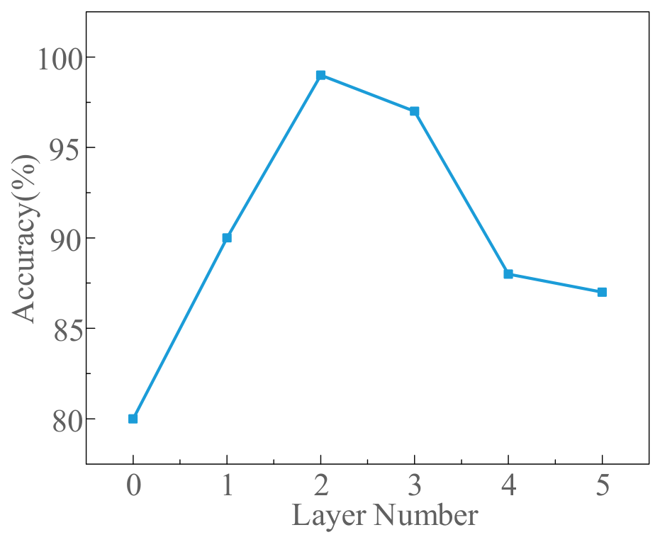
The graph branch of the proposed model consists of two GCN layers. The first layer fuses current and voltage features from directly connected nodes, while the second layer captures indirect relationships among the nodes. Because the constructed dynamic graph contains only six nodes, two GCN layers are sufficient to capture most relevant node relationships. Too few layers may limit information exchange, whereas too many layers can make node features overly similar and propagate noise. Therefore, a layer-wise ablation study was conducted, showing that two GCN layers provide a good balance between diagnostic accuracy and computational complexity.

Figure 13 shows that classification accuracy depends on GCN depth. A single layer produced poor performance, indicating insufficient extraction of fault-related graph features. Accuracy peaked at two layers but declined in deeper networks, likely because over smoothing reduced class separability and increased sensitivity to noise. Considering accuracy, model size, and computational cost, two GCN layers were therefore adopted.

4.2.4. Performance Evaluation Metrics

To quantitatively evaluate the effectiveness of the proposed fault diagnosis method, four metrics were employed to assess practicality and feasibility: accuracy, precision, recall, and F1 score. These metrics are defined as follows:

$$Accuracy={\displaystyle \frac{TP+TN}{TP+TN+FP+FN}}$$

(38)

$$Precision={\displaystyle \frac{TP}{TP+FP}}$$

(39)

$$Recall={\displaystyle \frac{TP}{TP+FN}}$$

(40)

$$F1-score=2\times {\displaystyle \frac{Precision\times Recall}{Precision+Recall}}$$

(41)

4.3. Ablation Experiment

4.3.1. Effectiveness Validation of the Sinkhorn–Wasserstein Dynamic Graph Construction Method

To evaluate the proposed Sinkhorn–Wasserstein weighted dynamic graph, comparing three graph construction strategies: a Euclidean distance KNN weighted graph, an unweighted Sinkhorn graph, and the proposed weighted dynamic graph. All strategies used the same node features, edge budget, GCN backbone, and optimization settings. Each experiment was repeated ten times, and the mean classification accuracy was recorded.

Table 6. Accuracy, training time, and number of parameters for models using different composition methods.

Model	Accuracy (%)	Mean Training Time (s)	Parameters (k)
Euclidean distance KNN weighted graph	92.34	11 s	20.12
Unweighted Sinkhorn graph	95.21	14 s	22.45
Proposed	99.88	15 s	25.34

summarizes the results.

As shown in Table 6, the Euclidean distance KNN graph has the lowest graph branch parameter count and training time because it directly constructs the adjacency matrix using pairwise Euclidean distances. The Sinkhorn-based methods require additional computational time to iteratively estimate entropy-regularized transport distances. The proposed weighted Sinkhorn method achieves the highest accuracy of 99.88%, with 25.34 K graph branch trainable parameters and a mean training time of 15 s. Compared with the Euclidean distance KNN graph, the proposed method improves accuracy by 7.54 percentage points at the cost of 5.22 K additional parameters and 4 s of training time. These results indicate that the proposed method provides a favorable accuracy–complexity trade-off rather than the lowest computational complexity.

4.3.2. Ablation Experiments for the Proposed Dual-Stream Model

To verify the effectiveness of each component of the proposed model, this paper conducts ablation experiments on the proposed dual-stream model using the control variable method. First, the graph convolutional branch and the temporal branch are retained separately to analyze the independent diagnostic capabilities of the two types of features. The parallel dual-stream model is then compared with the sequentially connected GCN-BiGRU model to verify the effectiveness of the parallel structure. The results are shown in

Table 7. Ablation results of the proposed dual-stream model.

Model	Accuracy (%)	Precision (%)	Recall (%)	F1-Score (%)
CNN-GCN	93.98 ± 4.00	94.10 ± 4.96	93.99 ± 4.20	93.97 ± 4.57
CNN-Sinkhorn-GCN	95.00 ± 1.80	95.09 ± 1.59	94.96 ± 1.60	95.01 ± 1.70
CNN-Sinkhorn-GCN + GRU	95.47 ± 1.93	96.60 ± 1.45	96.47 ± 1.83	96.46 ± 1.88
CNN-Sinkhorn-GCN + BiGRU	96.96 ± 1.61	97.96 ± 1.54	96.96 ± 1.41	96.96 ± 1.10
Proposed	99.88 ± 0.84	98.98 ± 1.24	98.88 ± 1.16	98.78 ± 2.0

.

Table 7 shows that using sample graphs constructed from the Sinkhorn-derived adjacency matrix improves the diagnostic metrics of CNN-GCN and reduces variation across repeated runs. Adding a parallel GRU branch provides temporal information but slightly increases result variation. Replacing GRU with BiGRU further improves diagnostic performance. The subsequent addition of global attention and parallel dual-stream fusion produces additional gains. These ablation results indicate that each component contributes to the final diagnostic performance.

4.3.3. Ablation Experiments of Global Attention Mechanism for the Proposed Dual-Stream Model

To verify the role of global attention in temporal branching and dual-stream models, this paper compares feature fusion methods for temporal features using global average pooling, fully connected layers, and global attention. The experimental results are shown in

Table 8. Validation results of global attention.

Model	Accuracy (%)
GRU + Global Average Pooling	87.78%
BiGRU + Global Average Pooling	90.34%
BiGRU + Full Connected	93.54%
GRU + Global Attention	95.65%
BiGRU + Global Attention	96.77%
Dual-branch + Full Connected	98.56%
Proposed	99.88%

.

After introducing global attention into the GRU architecture, the accuracy improved by 7.87 percentage points; in the BiGRU architecture, replacing global average pooling and the fully connected layer with global attention resulted in accuracy improvements of 6.43 and 3.23 percentage points, respectively. This indicates that simple pooling tends to weaken key fault features, while fully connected layers use relatively fixed feature mappings, making it difficult to dynamically adjust the importance of different time segments based on varying fault samples. By adaptively assigning weights, global attention highlights key fault information such as fault occurrence, waveform abrupt changes, and distinct differences between fault categories, while reducing the input of irrelevant fault features and noise interference.

Under the same attention mechanism, BiGRU achieved a further 1.12 percentage point improvement over the GRU, indicating that bidirectional contextual information and attention weighting have a complementary effect. In the dual-stream architecture, replacing the fully connected fusion with global attention resulted in a further improvement of 1.20 percentage points for the complete model, indicating that the attention mechanism can still generate independent gains after the fusion of graph space and temporal features rather than simply increasing the network’s complexity. Overall, the experimental results validate that global attention can improve the utilization efficiency of key fault features and is a crucial component for enhancing the classification performance of dual-stream models.

4.4. Comparison with State-of-the-Art Methods

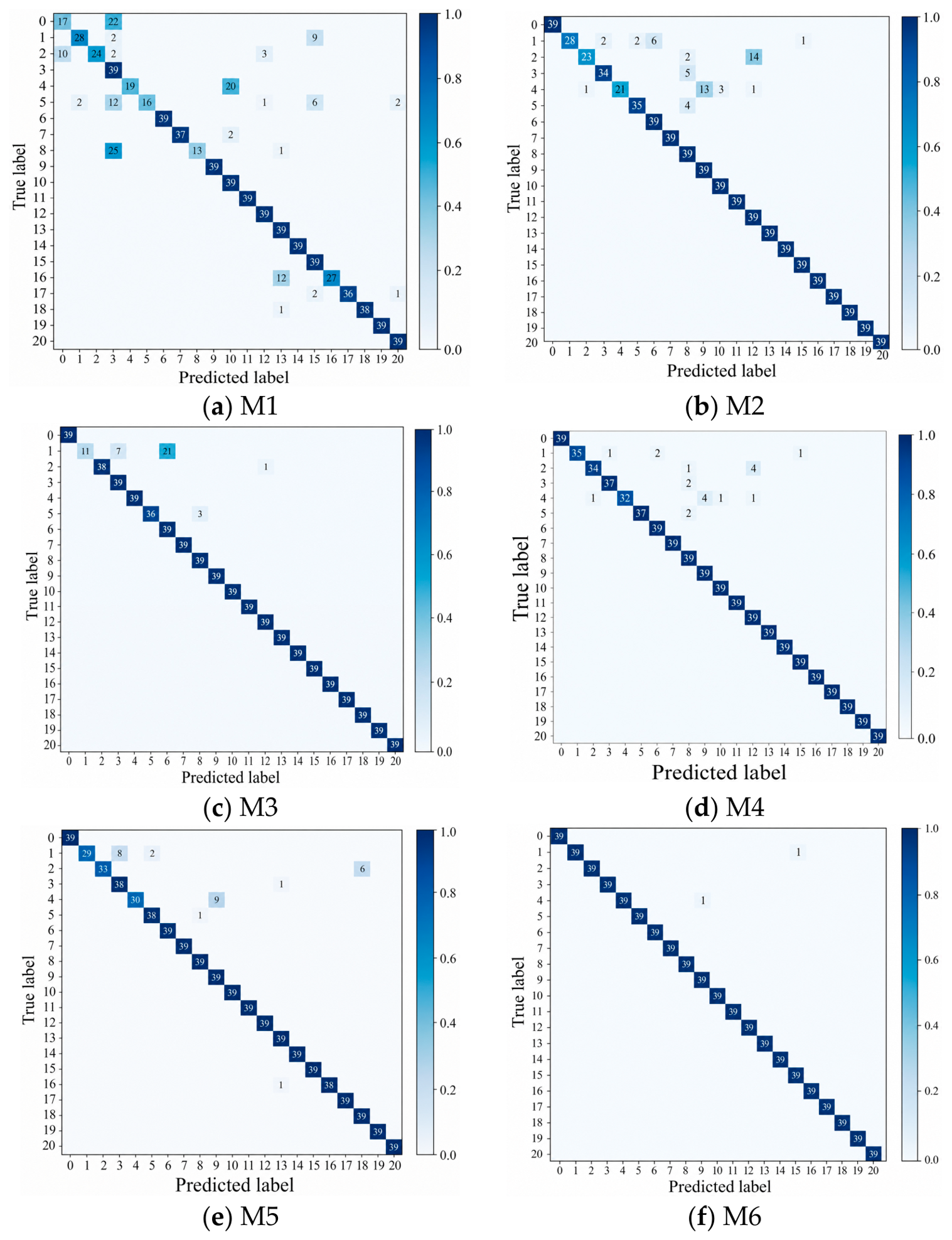
To facilitate comparison of the confusion matrices in Figure 14, M1–M5 represent TCN [11], CNN-SVM [12], SE-ResNet [15], MSSCNN [17], and 1D-DSCNN-GMP [16], respectively, while M6 denotes the proposed method. As shown in Figure 14, M1 and M2 contain more off-diagonal entries, indicating confusion between several fault classes. Misclassification is reduced for M3–M5. For M6, most predictions are concentrated on the main diagonal, with only a few misclassified samples, indicating effective discrimination among the 21 operating states.

Figure 14f shows that only two of the 819 validation samples were misclassified in the representative run: one class-1 sample was predicted as class 15, and one class-4 sample was predicted as class 9. According to Table 3, these errors correspond to S_a1S_a2 being predicted as S_a3S_a4 and S_a1S_b1 being predicted as S_a2S_a3. None of the errors involved the four single-IGBT faults S_a1, S_a2, S_a3, and S_a4, corresponding to labels 0, 8, 14, and 18. All 39 samples in each of these four classes were correctly identified without false-positive predictions, yielding both precision and recall of 100%. Although these single-IGBT faults cause related changes in the current conduction paths, they affect different current directions, half-cycle intervals, and switching state transitions. The joint current–voltage representation therefore provides complementary information for distinguishing these physically similar fault conditions. The representative run shown in Figure 14f achieved an accuracy of 99.76%, whereas the 99.88% value reported elsewhere is the mean accuracy across repeated runs.

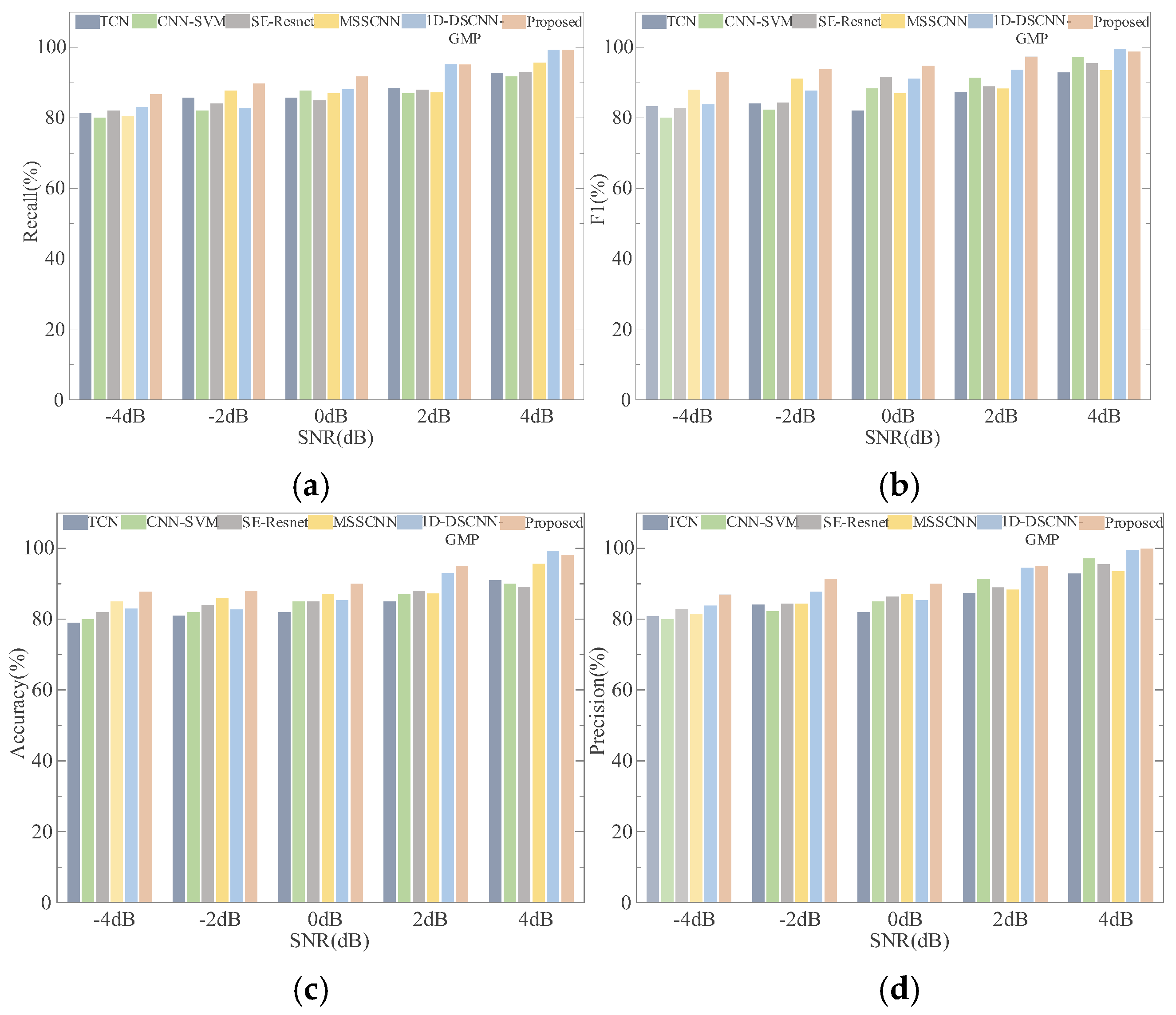
Figure 15 compares the six models under Gaussian white noise levels of −4 dB, −2 dB, 0 dB, 2 dB, and 4 dB. Figure 15a–d report accuracy, precision, recall, and F1-score, respectively. Under the 4 dB noise class, the proposed model performs slightly below 1D-DSCNN-GMP in accuracy and F1-score. Under the stronger noise conditions of −4 dB and −2 dB, however, it achieves the highest values across all four metrics, demonstrating strong noise robustness.

Under 4 dB, the relatively high SNR means that the original waveforms retain strong local discriminative features. Under this mildly corrupted condition, 1D-DSCNN-GMP can efficiently extract local patterns using depthwise separable convolutions, while global max pooling directly preserves the strongest discriminative responses. Therefore, this baseline remains particularly competitive, and the additional benefits of dynamic graph representation and temporal dependency modeling are less pronounced. In contrast, under the lower-SNR conditions of −4 and −2 dB, isolated local responses become less reliable, whereas the proposed method can exploit inter-signal relationships and temporal consistency to suppress unstructured noise, resulting in superior performance across all four metrics. Although Sinkhorn-based graph regularization may provide limited additional benefit under mild noise, the present results are insufficient to conclude that the graph becomes less discriminative relative to the signal variance. Accordingly, the robustness claim refers to the model’s overall stability and superior performance under severe noise rather than uniform superiority at every individual SNR level.

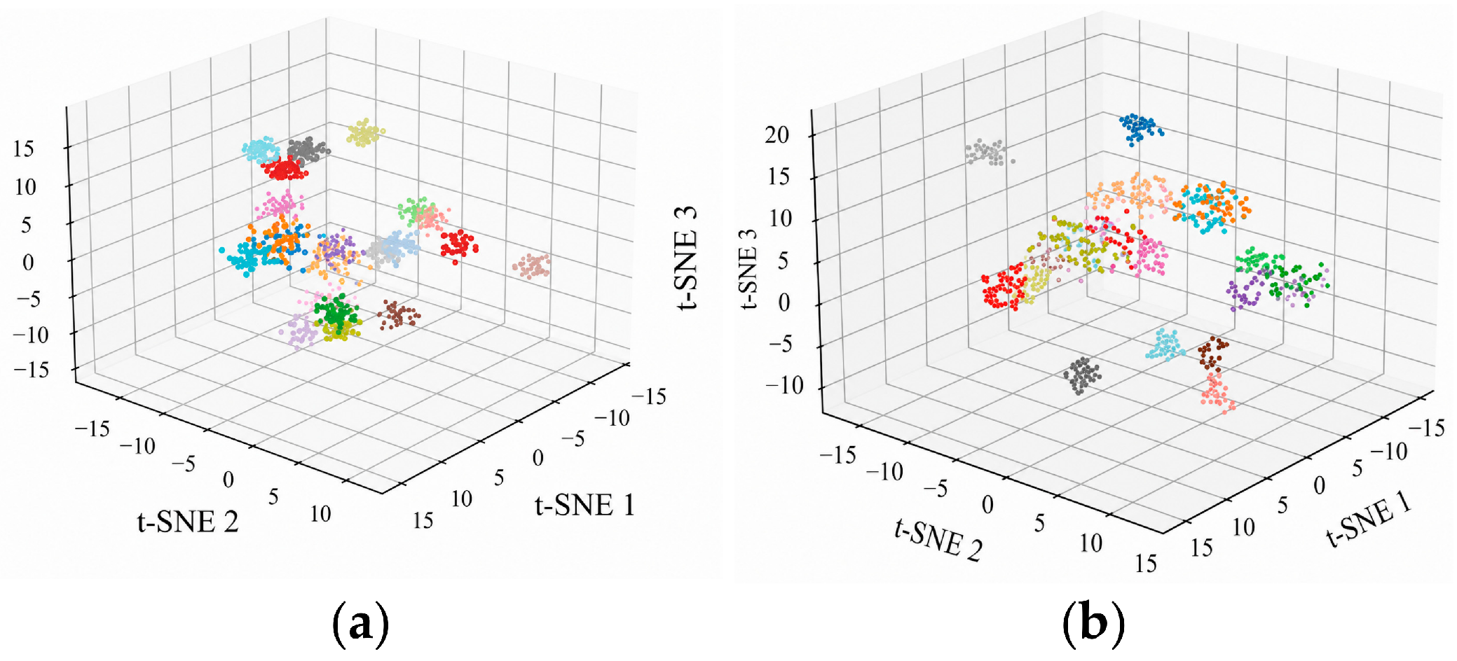
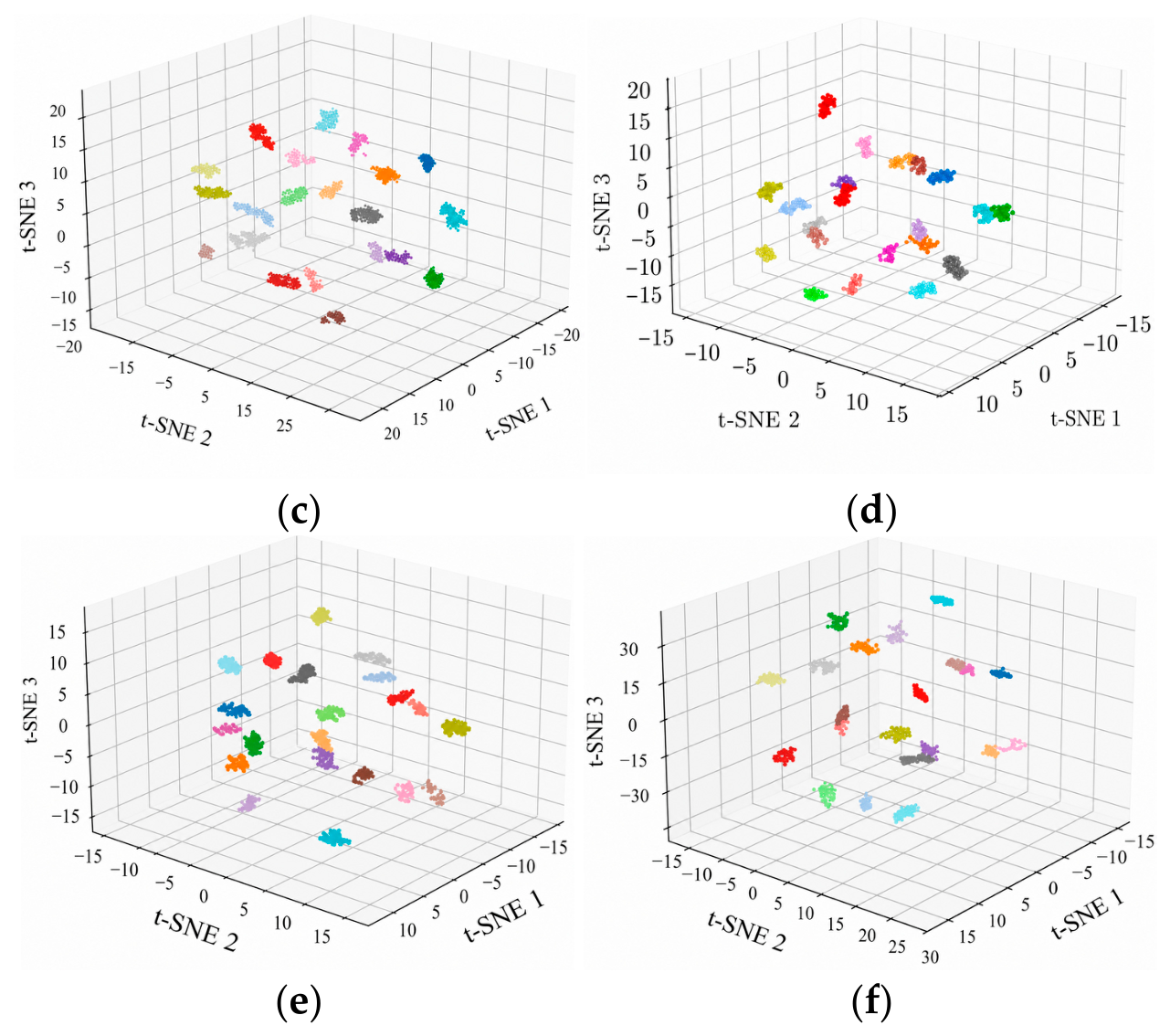
Figure 16 compares the t-SNE projections of validation set features learned by six models for 21 fault classes. Different colors denote different operating-condition classes, including the healthy condition and various fault categories. The same color coding is used consistently across Figure 16a–d. The proposed model produced compact well-separated clusters, whereas TCN showed considerable interclass overlap.

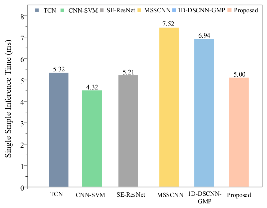
Figure 17 shows that CNN-SVM achieved the lowest latency, while MSSCNN and 1D-DSCNN-GMP required longer inference times. The average inference time of the proposed method was approximately 5 ms per diagnostic sample with a batch size of one. This value covers the complete model computation, including CNN feature extraction, Sinkhorn–Wasserstein-based dynamic graph construction, GCN and attention-based BiGRU processing, feature fusion, and final classification. Signal acquisition and data transmission time were not included. With high classification accuracy, the proposed model provided a favorable balance between diagnostic performance and computational efficiency.

5. Experiment Validation

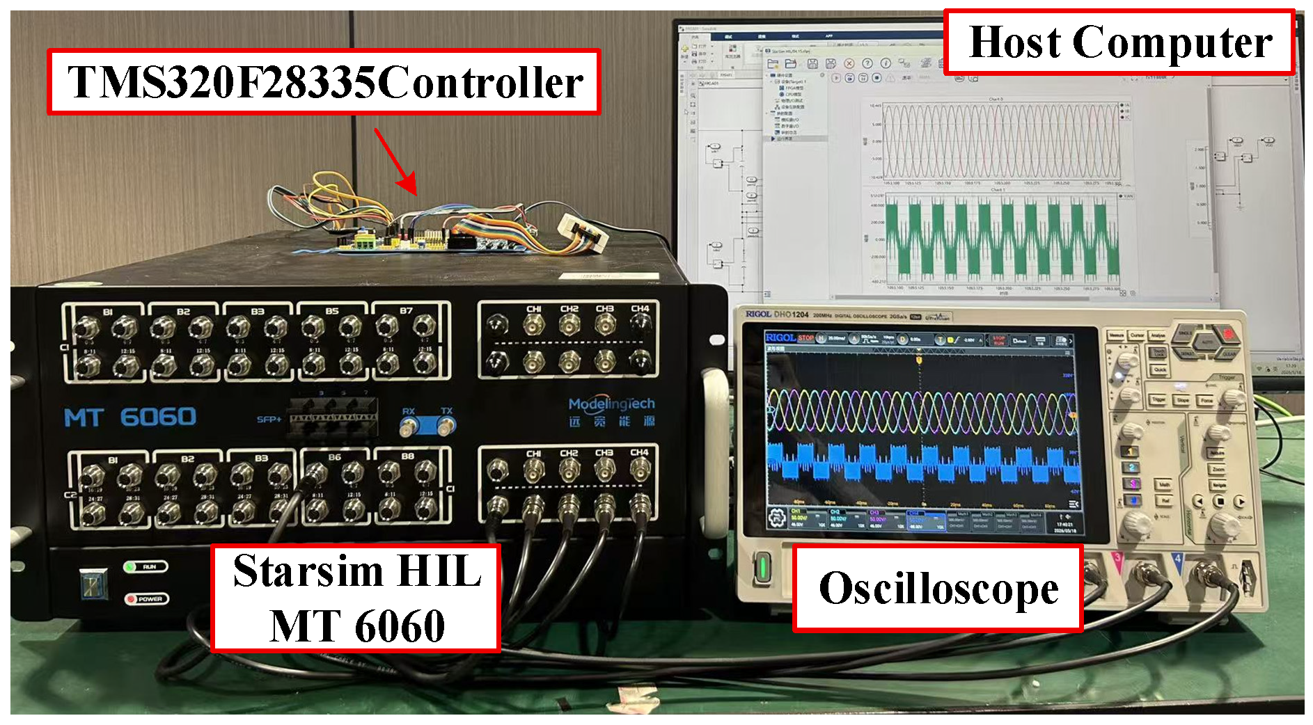
To further validate the feasibility of the proposed fault diagnosis method, a hardware-in-the-loop experimental platform was set up, as shown in Figure 18. The computer transferred the T-NPC converter model to the real-time simulator Starsim MT6060 (Shanghai, China). The TMS320F28335 DSP generates 20 kHz PWM control signals, which are received by Digital I/O of the MT6060 real-time simulator. The analog output is i_a, i_b, i_c, V_AN, V_BN, V_CN to TMS320F28335 for establishing datasets. The experimental parameters are shown in

Table 9. Experimental parameters.

Notation	Parameters	Values
$U_{\mathit{dc}}$	DC side voltage	800 V
C1, C2	DC side capacitance	4000 µF
$f_s$	Switching frequency	20 kHz
$R$	Load resistance	30 Ω
$L_f$	Filter inductors	3 mH
$C_f$	Filter capacitor	8000 µF

.

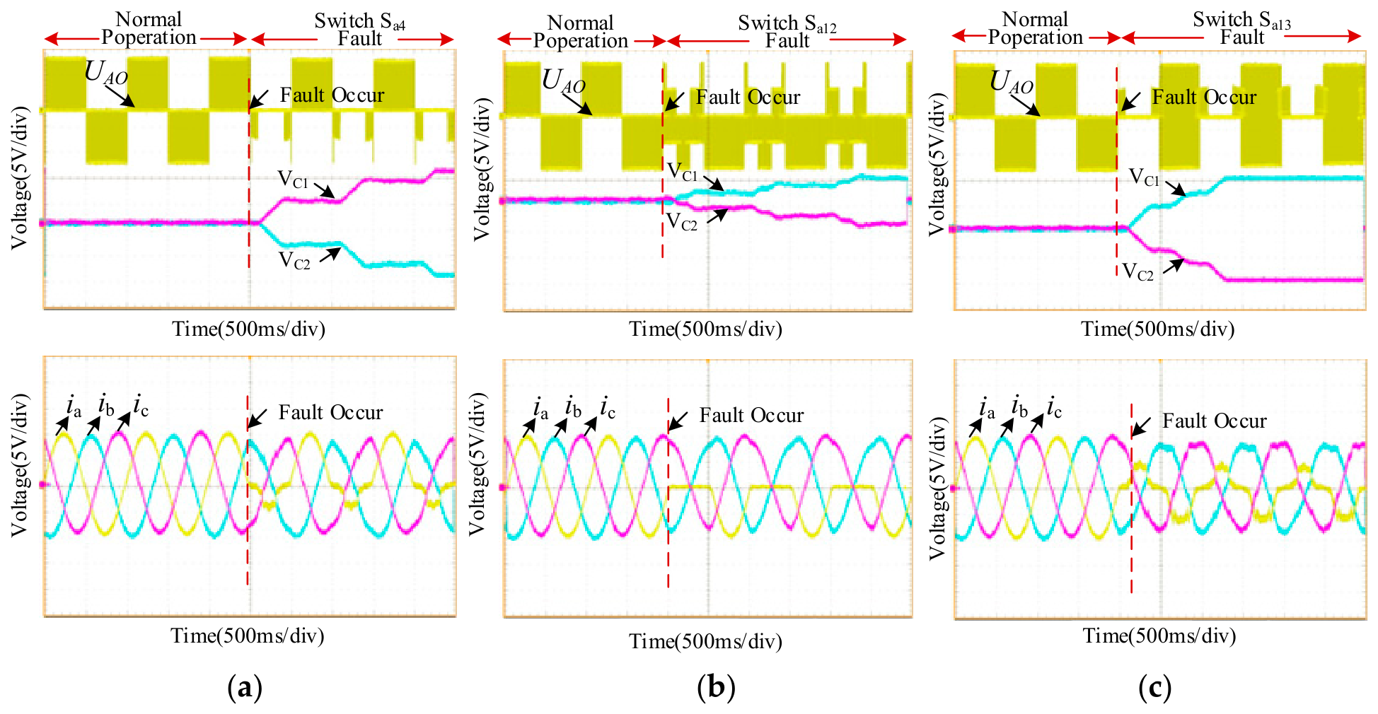
Figure 19 shows the experimental voltage and current waveforms when different switching devices fail. When different switching devices experience varying degrees of failure, both the U_AO and the i_a, i_b, and i_c signals exhibit varying degrees of distortion. Therefore, when S_a1 fails, waveform distortion occurs in both the U_AO and the i_a, i_b, and i_c signals. As shown in Figure 19a, when S_a4 experiences an open-circuit fault, the U_AO waveform becomes distorted during the second half-cycle. Since the voltage V_C1 across the upper and lower capacitors is greater than V_C2, the ia component of the three-phase currents i_a, i_b, and i_c also exhibits waveform distortion in the second half-cycle. The analysis of open-circuit faults in other IGBTs follows a similar pattern, consistent with the simulation results, thereby validating the correctness of the fault mechanism analysis. At the same time, different fault states exhibit distinct characteristics in the multi-channel current and voltage signals, indicating that the acquired signals exhibit distinct characteristics when a fault occurs.

6. Conclusions

This study proposed a parallel graph–temporal network for diagnosing 21 IGBT open-circuit operating states in a T-NPC three-level inverter. The complete model achieved an accuracy of 99.88% on the validation set compared with 93.99% for the CNN-GCN model and 95.01% for the CNN–Sinkhorn–GCN model. Moreover, replacing fully connected feature fusion with global attention increased the accuracy from 98.56% to 99.88%. These results indicate that the Sinkhorn-weighted dynamic graph captures sample-dependent relationships among the voltage and current signals, while the attention-based BiGRU emphasizes fault-relevant temporal patterns. The parallel fusion of relational and temporal features therefore provides complementary information for fault classification. The HIL platform was used to reproduce different IGBT fault conditions and acquire experimental voltage and current signals, supporting the feasibility of the fault condition reproduction and data acquisition process. Future work will investigate cross-condition generalization, model complexity reduction, HIL-only quantitative evaluation, and real-time deployment on embedded hardware.

References

1. Chen, S.; Liu, P.; Li, Z. Low carbon transition pathway of power sector with high penetration of renewable energy. Renew. Sustain. Energy Rev. 2020, 130, 109985. [Google Scholar] [CrossRef] [Scilit]
2. Zhang, Z.; Anthon, A.; Andersen, M.A.E. Comprehensive loss evaluation of neutral-point-clamped (NPC) and T-type three-level inverters based on a circuit-level decoupling modulation. In Proceedings of the 2014 International Power Electronics and Application Conference and Exposition (PEAC), Shanghai, China, 5–8 November 2014; pp. 82–87. [Google Scholar]
3. Wang, B.; Cai, J.; Du, X.; Zhou, L. Review of power semiconductor device reliability for power converters. CPSS Trans. Power Electron. Appl. 2017, 2, 101–117. [Google Scholar] [CrossRef] [Scilit]
4. Song, Y.; Wang, B. Survey on reliability of power electronic systems. IEEE Trans. Power Electron. 2013, 28, 591–604. [Google Scholar] [CrossRef] [Scilit]
5. Mullali Kunnontakath Puthiyapurayil, M.R.; Nadir Nasirudeen, M.; Saywan, Y.A.; Ahmad, M.W.; Malik, H. A review of open-circuit switch fault diagnostic methods for neutral-point-clamped inverter. Electronics 2022, 11, 3169. [Google Scholar] [CrossRef] [Scilit]
6. Jlassi, I.; Estima, J.O.; El Khil, S.K.; Bellaaj, N.M.; Cardoso, A.J.M. A robust observer-based method for IGBTs and current sensors fault diagnosis in voltage-source inverters of PMSM drives. IEEE Trans. Ind. Appl. 2017, 53, 2894–2905. [Google Scholar] [CrossRef] [Scilit]
7. Luo, Y.; Zhang, L.; Chen, C.; Li, K.; Yu, T.; Li, K. FRA-based parameter estimation for fault diagnosis of three-phase voltage-source inverters. IEEE Access 2023, 11, 113836–113847. [Google Scholar] [CrossRef] [Scilit]
8. Zhang, W.; He, Y.; Chen, J. A robust open-circuit fault diagnosis method for three-level T-type inverters based on phase voltage vector residual under modulation mode switching. IEEE Trans. Power Electron. 2023, 38, 5309–5322. [Google Scholar] [CrossRef] [Scilit]
9. Kou, L.; Liu, C.; Cai, G.; Zhou, J.; Yuan, Q.; Pang, S. Fault diagnosis for open-circuit faults in NPC inverter based on knowledge-driven and data-driven approaches. IET Power Electron. 2020, 13, 1236–1245. [Google Scholar] [CrossRef] [Scilit]
10. Chen, X.; Zhang, Z. Open-circuit fault diagnosis of T-type three-level inverter based on knowledge reduction. Sensors 2024, 24, 1028. [Google Scholar] [CrossRef] [Scilit] [PubMed]
11. Li, G.; Li, J.; He, Y.; Guo, Q. Fault diagnosis method of three-phase inverter based on time convolutional neural network. Recent Adv. Electr. Electron. Eng. 2022, 15, 401–409. [Google Scholar] [CrossRef] [Scilit]
12. Tian, L.; Zhang, H.; Hu, B.; Yu, Q. Fault diagnosis of three-level inverter based on convolutional neural network and support vector machine. J. Chin. Inst. Eng. 2023, 46, 829–838. [Google Scholar] [CrossRef] [Scilit]
13. Cui, Y.; Wang, R.; Si, Y.; Zhang, S.; Wang, Y.; Lin, A. T-type inverter fault diagnosis based on GASF and improved AlexNet. Energy Rep. 2023, 9, 2718–2731. [Google Scholar] [CrossRef] [Scilit]
14. Yan, J.; Huang, Y.; Yuan, S.; Lu, Y.; Yu, Z. Open-circuit fault analysis and recognition in three-level inverters based on recurrence plot and convolution neural network. Int. Trans. Electr. Energy Syst. 2023, 2023, 4755960. [Google Scholar] [CrossRef] [Scilit]
15. Fu, Y.; Ji, Y.; Meng, G.; Chen, W.; Bai, X. Three-phase inverter fault diagnosis based on an improved deep residual network. Electronics 2023, 12, 3460. [Google Scholar] [CrossRef] [Scilit]
16. Xie, F.; Tang, X.; Xiao, F.; Luo, Y.; Shen, H.; Shi, Z. Online diagnosis method for open-circuit fault of NPC inverter based on 1D-DSCNN-GMP lightweight edge deployment. IEEE J. Emerg. Sel. Top. Power Electron. 2023, 11, 6054–6067. [Google Scholar] [CrossRef] [Scilit]
17. Yan, Y.; Wu, J.; Cao, Y.; Liu, B.; Li, C.; Shi, T. An open-circuit fault diagnosis method for three-level neutral-point-clamped inverters based on multi-scale shuffled convolutional neural network. Sensors 2024, 24, 1745. [Google Scholar] [CrossRef] [Scilit] [PubMed]
18. Yang, W.; Wang, W.; Wang, X.; Gu, J.; Wang, Z. Fault diagnosis method of a cascaded H-bridge inverter based on a multisource adaptive fusion CNN-transformer. IET Power Electron. 2024, 17, 2289–2304. [Google Scholar] [CrossRef] [Scilit]
19. Xing, Z.; He, Y.; Zhang, W. An online multiple open-switch fault diagnosis method for T-type three-level inverters based on multimodal deep residual filter network. IEEE Trans. Ind. Electron. 2023, 70, 10669–10679. [Google Scholar] [CrossRef] [Scilit]
20. Xia, Y.; Xu, Y. A robust data-driven method for open-circuit fault diagnosis of power switches in three-phase inverters with low-quality data. IEEE Trans. Power Electron. 2024, 40, 5949–5958. [Google Scholar] [CrossRef] [Scilit]
21. Xia, Y.; Xu, Y.; Zhou, N. A transferrable and noise-tolerant data-driven method for open-circuit fault diagnosis of multiple inverters in a microgrid. IEEE Trans. Ind. Electron. 2024, 71, 8017–8027. [Google Scholar] [CrossRef] [Scilit]
22. Guan, Y.; Meng, Z.; Gu, F.; Cao, Y.; Li, D.; Miao, X.; Ball, A.D. Fault diagnosis of wind turbine structures with a triaxial vibration dual-branch feature fusion network. Reliab. Eng. Syst. Saf. 2025, 256, 110746. [Google Scholar] [CrossRef] [Scilit]
23. Yan, P.; Zheng, S.; Huang, Z.; Peng, L.; Liu, J.; Wang, D. SOM-DBTGNet: A hybrid PV fault diagnosis method integrating self-organizing maps and dual-branch temporal graph convolution network. Process Saf. Environ. Prot. 2025, 204, 108148. [Google Scholar] [CrossRef] [Scilit]
24. Dong, Y.; Liu, J.; Chen, Y.; Chen, G.; Zhang, F.; Gao, J. Data-driven fault diagnosis for autonomous underwater vehicles using lag-aware spatio-temporal dynamic graph networks. Ocean Eng. 2026, 356, 125146. [Google Scholar] [CrossRef] [Scilit]
25. Li, T.; Zhao, Z.; Sun, C.; Yan, R.; Chen, X. Multireceptive field graph convolutional networks for machine fault diagnosis. IEEE Trans. Ind. Electron. 2021, 68, 12739–12749. [Google Scholar] [CrossRef] [Scilit]
26. Gao, Y.; Chen, M.; Yu, D. Semi-supervised graph convolutional network and its application in intelligent fault diagnosis of rotating machinery. Measurement 2021, 186, 110084. [Google Scholar] [CrossRef] [Scilit]
27. Zhang, X.; Hu, Y.; Liu, J.; Zhang, X.; Wu, B. Robust rotating machinery diagnosis using a dynamic-weighted graph updating strategy. Measurement 2022, 202, 111895. [Google Scholar] [CrossRef] [Scilit]
28. Xiao, S.; Hou, J.; Khan, M.J.; Sun, B. CDGCN: A CNN-enhanced dynamic graph convolutional network for multimodal fault diagnosis. Measurement 2026, 269, 120788. [Google Scholar] [CrossRef] [Scilit]
29. LeCun, Y.; Bottou, L.; Bengio, Y.; Haffner, P. Gradient-Based Learning Applied to Document Recognition. Proc. IEEE 1998, 86, 2278–2324. [Google Scholar] [CrossRef] [Scilit]
30. Sinkhorn, R. A Relationship Between Arbitrary Positive Matrices and Doubly Stochastic Matrices. Ann. Math. Stat. 1964, 35, 876–879. [Google Scholar] [CrossRef] [Scilit]
31. Cuturi, M. Sinkhorn Distances: Lightspeed Computation of Optimal Transport. Adv. Neural Inf. Process. Syst. 2013, 26, 2292–2300. [Google Scholar]
32. Peyré, G.; Cuturi, M. Computational Optimal Transport: With Applications to Data Science. Found. Trends Mach. Learn. 2019, 11, 355–607. [Google Scholar] [CrossRef] [Scilit]
33. Kipf, T.N.; Welling, M. Semi-Supervised Classification with Graph Convolutional Networks. In Proceedings of the International Conference on Learning Representations (ICLR), Toulon, France, 24–26 April 2017. [Google Scholar]
34. Cho, K.; van Merriënboer, B.; Gulcehre, C.; Bahdanau, D.; Bougares, F.; Schwenk, H.; Bengio, Y. Learning Phrase Representations Using RNN Encoder–Decoder for Statistical Machine Translation. In Proceedings of the Empirical Methods in Natural Language Processing, Doha, Qatar, 25–29 October 2014; pp. 1724–1734. [Google Scholar]
35. Schuster, M.; Paliwal, K.K. Bidirectional Recurrent Neural Networks. IEEE Trans. Signal Process. 1997, 45, 2673–2681. [Google Scholar] [CrossRef] [Scilit] [PubMed]
36. Luong, M.-T.; Pham, H.; Manning, C.D. Effective Approaches to Attention-Based Neural Machine Translation. In Proceedings of the Empirical Methods in Natural Language Processing, Lisbon, Portugal, 17–21 September 2015; pp. 1412–1421. [Google Scholar]
Figure 1. Three-level T-NPC converter topology.
Energies 19 04227 g001
Figure 2. The current path in the Sa1 and Sa3 or Sa4 single-IGBT open-circuit fault of phase-A.
Energies 19 04227 g002
Figure 3. The Structure of the Spatial feature extract-based graph convolutional network module.
Energies 19 04227 g003
Figure 4. The procedure of a graph convolutional network.
Energies 19 04227 g004
Figure 5. The Structure of temporal feature extraction based on BiGRU with global attention.
Energies 19 04227 g005
Figure 6. The structure of BiGRU.
Energies 19 04227 g006
Figure 7. The structure of global attention.
Energies 19 04227 g007
Figure 8. The structure of global attention BiGRU.
Energies 19 04227 g008
Figure 9. Spatial feature and temporal feature fusion.
Energies 19 04227 g009
Figure 10. Simulation waveforms of IGBT open-circuit fault in phase-A. (a) Sa1 open-circuit fault. (b) Sa2 open-circuit fault. (c) Sa3 open-circuit fault. (d) Sa4 open-circuit fault. (e) Sa1Sa2 open-circuit fault. (f) Sa1Sa3 open-circuit fault.
Energies 19 04227 g010
Figure 11. The training curves of the proposed dual-stream model.
Energies 19 04227 g011
Figure 12. Effect of entropy regularization parameter on classification accuracy.
Energies 19 04227 g012
Figure 13. Effect of GCN layer number on classification accuracy.
Energies 19 04227 g013
Figure 14. Comparison of confusion matrices of state-of-the-art models.
Energies 19 04227 g014
Figure 15. Classification results of different fault diagnosis models under varying Gaussian white noise levels: (a) recall; (b) F1-score; (c) accuracy; (d) precision.
Energies 19 04227 g015
Figure 16. T-SNE visualization evaluation on different models. (a) TCN. (b) CNN-SVM. (c) SE-ResNet. (d) MSSCNN. (e) 1D-DSCNN-GMP. (f) Proposed method.
Energies 19 04227 g016aEnergies 19 04227 g016b
Figure 17. Comparison of inference latency among different fault diagnosis models.
Energies 19 04227 g017
Figure 18. Experimental structure and platform of the hardware-in-the-loop system.
Energies 19 04227 g018
Figure 19. Experimental results of IGBT open-circuit fault. (a) Sa4 open-circuit fault. (b) Sa1Sa2 open-circuit fault (c) Sa1Sa3 open-circuit fault.
Energies 19 04227 g019