Article

Resilience Planning for Coupled Power–Transportation Systems Based on Scenario-Feature Identification and Adversarial Reinforcement Learning

1
Grid Planning Research Center, Guangdong Power Grid Co., Ltd., Guangzhou 510062, China
2
Zhanjiang Power Supply Bureau, Guangdong Power Grid Co., Ltd., Zhanjiang 524000, China
3
Jiangmen Power Supply Bureau, Guangdong Power Grid Co., Ltd., Jiangmen 529000, China
4
Shantou Power Supply Bureau, Guangdong Power Grid Co., Ltd., Shantou 515000, China
5
Department of Mechanical Engineering, North China Electric Power University, Baoding 071003, China
*
Author to whom correspondence should be addressed.
Energies 2026, 19(17), 4078; https://doi.org/10.3390/en19174078
Submission received: 4 June 2026 / Revised: 25 July 2026 / Accepted: 27 August 2026 / Published: 30 August 2026
(This article belongs to the Section A1: Smart Grids and Microgrids)

Abstract

New loads, represented by electric vehicles, are emerging rapidly. Distribution networks therefore face increasingly complex spatiotemporal load fluctuations. Conventional planning methods inadequately consider traffic factors. They also overlook traffic-induced dynamic load variations. Accordingly, this study proposes a traffic load-coupled planning method for distribution networks. The primary novelty lies in identifying load features. It also uses classified scenarios as model inputs. This design reveals nonlinear impacts of dynamic traffic flow transfers on grid resilience across functional scenarios. First, load-feature clustering identifies scenario attributes for nodes, power lines, and traffic roads. Second, classified scenarios and historical data are used as model inputs. An improved model then generates high-confidence prediction intervals for power load and traffic flow. A dynamic mapping model is established between traffic flow and nodal power load. Then, adversarial reinforcement learning is used to obtain the planning scheme. An attack–defense game further enhances robustness under extreme disturbances. Finally, comparative simulations verify the superiority of the proposed scheme.

1. Introduction

As the global energy transition and transport electrification accelerate, distribution network load profiles are changing. Electric vehicles (EVs) are no longer merely an emerging electricity load. They are evolving into a key source of uncertainty that shapes the long-term planning boundary of distribution networks [1]. The IEA’s “Global EV Outlook 2025” provides projections under the Stated Policies Scenario (STEPS). Under this scenario, the global EV stock is forecast to reach approximately 250 million by 2030. This figure is roughly four times the stock at the end of 2024. This indicates that transport electrification introduces incremental demand and fluctuations on the distribution side. These impacts represent long-term certainties [2,3].
However, large-scale uncoordinated EV charging poses significant challenges to distribution network stability [4,5]. Srivastava et al. systematically reviewed the power quality issues arising from EV integration, such as voltage deviation, voltage imbalance, and harmonics, along with the corresponding mitigation techniques. They further highlighted the comprehensive nature of distribution-side operational risks under high-penetration scenarios [6]. However, these studies mainly treat EV charging demand as a simple fluctuating load at a single node. They focus on static impact assessment and short-term control.
EV load uncertainty arises not only from random arrivals and charging power. It is also driven by transportation network dynamics and heterogeneous user behavior. Powell et al. proposed a scalable probabilistic method for estimating charging demand from observed driving behavior. They used clustering to characterize heterogeneity in drivers’ charging behavior. This approach provides a data-driven basis for constructing multi-scenario demand in long-term planning [7]. For short-term forecasting, Wang et al. developed a heterogeneous spatiotemporal graph convolutional network. The network predicts the spatiotemporal distribution of charging demand [8]. Several studies show that traffic, geographic, and demand graphs improve user load profiling. They also enhance forecasting accuracy [8,9,10]. Pentsos et al. and Hu et al. investigated probabilistic forecasting to further improve prediction accuracy [11,12].
Research on coordinated optimization between power systems and other sectors has advanced substantially in recent years. Wang et al. [13] developed a multi-network cascading-failure model. The model captures dependencies between power and stormwater drainage networks. Guo et al. [14] proposed a dynamic aggregation-based emergency dispatch strategy. The strategy coordinates flexibility resources across power and water systems. It thereby mitigates power shortages during droughts. Zhou et al. [15] characterize power–transportation network equilibrium using a potential-game formulation. They jointly modeled drivers’ routing and charging choices with distribution network operating states. They also developed a decomposition-based solution method. Liang et al. [16] further propose a vehicle-to-grid (V2G) planning framework incorporating EV user equilibrium (UE). The framework jointly optimizes charging-facility siting and sizing. It simultaneously enhances distribution network flexibility. Shi et al. [17] considered distribution-side constraints, including three-phase imbalance. They proposed a distributed framework for coordinating distribution network and urban transportation planning.
Adversarial reinforcement learning (ARL) provides an effective approach for solving complex coupled problems. ARL converts extreme disturbances from predefined empirical scenarios into learnable adversarial strategies. Guo et al. explicitly introduce an optimal adversary into multi-agent deep reinforcement learning. They then conducted robust training. Their results show that min–max games approximate worst-case state perturbations. This process improves policy robustness [18]. Zhi proposed an efficient progressive polyhedral approximation method to reduce solution time [19]. Gao et al. studied control systems subject to dynamic uncertainty and denial-of-service attacks. They proposed a resilient reinforcement-learning method with robust output regulation. They also provided a framework for theoretical analysis and formal verification [20]. Zhou et al. investigated adversarial attacks in continuous action spaces. They identified critical agents and constructed worst-case joint actions. These attacks substantially degrade multi-agent policy performance. These results reveal the amplification effect of coordinated perturbations. This effect requires careful consideration in coupled transportation and power systems [21]. Ren et al. quantified adversarial-example-induced classification distortion in short-term voltage stability assessment. They further improve model robustness through adversarial training. This process enhances the reliability of critical infrastructure models [22]. Systematic reviews have also examined adversarial attacks and defense strategies in network security and intelligent systems. These reviews provide a general foundation for the adversarial perturbation model developed here [23]. However, most studies focus on robustness evaluation in operational control or individual learning tasks. They do not systematically capture the gap between planned investments and actual dispatch conditions. In particular, they struggle to address substantial real-world uncertainty under adverse conditions.
Distributionally robust reinforcement learning and ARL effectively characterize worst-case disturbances and adversarial strategies. They offer a tractable paradigm for robust decision-making in complex systems. Neufeld and Sester proposed robust Q-learning for Wasserstein ambiguity sets. They provide convergence analysis and numerical examples. Their work provides a feasible approach to approximating worst-case dynamics under distribution shifts [24]. Li and Shapiro examine rectangularity, duality, and game-based and static formulations in distributionally robust MDPs. Their analysis supports embedding uncertainty into dynamic programming or learning through attack–defense games [25]. For power-system security, Selim et al. formulated post-attack distribution network defense as a Markov decision process (MDP). They use deep reinforcement learning to enable adaptive defense decisions. Their results confirm the applicability of attack–defense modeling in power systems [26]. However, existing studies mainly address short-term operation under fixed network structures. They do not capture interactions between long-term investment planning and actual dispatch. This limitation is especially relevant to deeply coupled power–transportation systems.
Existing planning methods inadequately capture EV-induced dynamic loads. Extreme-weather data also remain scarce. This study proposes an adversarial robust planning model for coupled power–transportation networks. It also develops a corresponding solution method. The main contributions are as follows:
First, a deeply coupled power–transportation model captures the spatiotemporal dynamics of traffic flow. The model overcomes the conventional treatment of EVs as isolated stochastic loads. It quantifies the nonlinear effects of traffic flow redistribution on spatiotemporal grid loads.
Second, a scenario-informed interval forecasting method is proposed. For the first time, scenario classification results serve as explicit input features. These features are combined with historical load data for forecasting. Simulation results demonstrate the superior forecasting performance of this method.
Third, an ARL-based robust grid-planning method is developed. The method establishes a defender–attacker game. The defender uses policy gradients to optimize line and substation investments. The attacker searches for worst-case load–traffic flow combinations within data-supported intervals. The resulting plans remain effective under historical conditions. They also improve resilience to potential extreme weather. The method addresses computational complexity and limited extreme-weather data.
The remainder of this paper is structured as follows. Section 2 develops a capacity-planning model integrating scenario identification, interval forecasting, and power–transportation coupling. Section 3 presents the ARL-based solution framework. Section 4 evaluates the effectiveness and performance of the proposed method through case studies. Section 5 summarizes the main findings and contributions.

2. Configuration Planning Model Considering Power–Transportation Coupling

This study develops a coordinated modeling framework integrating data-driven methods with physical mechanisms. It enhances the resilience of urban power–transportation systems under extreme disturbances. A fully automatic density-based clustering method addresses cross-infrastructure data heterogeneity. Nodal loads, line-loading rates, and road traffic flows are dynamically segmented. Trend and statistical features are then extracted from each segment. A reference time-series is selected for centroid matching across the three data types. This process aligns the heterogeneous timeseries into corresponding scenario classes.
Building on this framework, an LSTM–Transformer model with quantile regression is developed. The LSTM–Transformer extracts temporal features from power loads and traffic flows. Quantile regression estimates conditional quantiles and constructs prediction intervals. Together, these components enable accurate interval forecasts of future loads and traffic flows. Meanwhile, a coupled indicator system characterizes operational risk. It includes nodal load ratios, distribution-line loading ratios, and traffic delays. The three-sigma rule classifies these indicators into multiple risk levels. A multilevel penalty mechanism then balances economic efficiency and operational security. Finally, a capacity planning model is established for resilience enhancement. The model follows a three-stage logic of investment, evaluation, and optimization. Coordinated decisions are then made to reinforce key power lines, expand traffic corridors, and increase charging-node capacity. These decisions enhance the robustness of the power–transportation-coupled network under extreme scenarios. They also support optimal resource allocation.

2.1. Feature Identification and Differentiated Scenario Classification of Power Load and Traffic Flow Based on Fully Automatic Density-Based Clustering

2.1.1. Hierarchical Processing of Temporal Features

The study objects include two types of infrastructure elements: nodes and links. The operation or usage behavior of different objects can be uniformly characterized by time-series. For load nodes, the behavior is represented by nodal load-power time-series. For distribution lines, the behavior is represented by line-loading-rate time-series. For road links, the behavior is represented by traffic-flow time-series.
Therefore, the original behavior of any node or link can be abstracted as a one-dimensional time-series: X = { x 1 , x 2 , x v } .
To eliminate scale differences and mitigate noise effects, min–max normalization is first applied to the time-series, as shown in Equation (1):
x v = x v x min x max x min
In Equation (1), xv denotes the original data. xmax and xmin denote the maximum and minimum values within the statistical period, respectively. x v denotes the normalized sequence.
Furthermore, sliding-window averaging is used to smooth the normalized sequence. This step mitigates the effect of short-term random disturbances on feature extraction. Let w denote the half-window length. The calculation is shown in Equation (2).
x m , v = 1 n j = w w x m , v + j
In Equation (2), w = 2. Node and link behaviors are usually nonstationary. Direct analysis of the complete time-series may obscure local behavioral features. Therefore, a time-series segmentation method based on a dynamically growing window is adopted.
A time-series with length III is dynamically segmented. The time-series is divided into mf segments. Accordingly, mf − 1 segmentation points are identified t = t q q = 1 1 . Time-series data are then introduced point by point into the dynamically growing window. The fitting error SSEq is calculated in real-time. The threshold SEPmax is set according to the overall noise level of the original sequence. When the error within the window exceeds the preset threshold SEPmax, the current time point is identified as the segmentation point tv. The current segment is then terminated, and a new segment is initialized. The initial segment t 0 = 1 is set to start from the beginning of the sequence. When the segmentation point t 1 = n is detected, the first n data points are assigned to the first segment. The range of the current segment is defined using the segmentation-point set t 1 , t 2 , , t m 1 . Thus, segment q is expressed in t q 1 + 1 , t q .
For each time-series segment, low-dimensional features are extracted from two aspects. These aspects include trend characteristics and statistical characteristics. Trend characteristics are obtained by fitting each segment with a low-order polynomial. The fitting coefficients reflect the overall trend of the segment. Statistical characteristics are represented by variance, skewness, and the autocorrelation coefficient. Their calculation formulas are shown in Equations (3)–(5).
S q 2 = 1 t q t q 1 + 1 v = t q 1 t q x v x ¯ q 2
γ 1 q = 1 t q t q 1 + 1 v = t q 1 t q x v x ¯ q 3 σ ^ q 3
A C q = v = t q 1 t q x v x ¯ q · x + 1 x ¯ q S q 2
The above features are combined to obtain the low-dimensional feature vector of each segment, as shown in Equation (6).
A C q = v = t q 1 t q x v x ¯ q · x + 1 x ¯ q S q 2
In Equation (6), pq denotes the polynomial approximation parameters of segment q.
To unify the feature dimensions of different nodes and links, hierarchical clustering is performed on all segment features. These features are then divided into a fixed number of behavioral categories. For each segment category, the cluster centroid and extreme segments C ¯ i j are extracted. Here, i 1 , , T denotes the time-series index, and T denotes the number of time-series. j 1 , , k denotes the cluster index in each time-series, and k denotes the number of clusters. Subsequently, one time-series is selected as the reference. Its segment clustering results are matched with the cluster centroids of other time-series. Cross-object category alignment is then completed. Each original timeseries is further mapped into a sequence composed of category labels X i . The above method provides fundamental inputs for subsequent differentiated scenario analysis and the coordinated decision-making model of nodes and links.

2.1.2. Fully Automatic Density-Based Clustering Algorithm

Through hierarchical temporal-feature processing, high-dimensional nonstationary time-series are transformed. These series are from the original nodes and links. They are converted into structurally unified low-dimensional feature representations. Based on local density distributions in the feature space, a fully automatic adaptive density-based clustering method is introduced. This method robustly identifies behavioral categories of nodes and links. Specifically, it identifies residential, commercial, and industrial patterns under holiday and non-holiday scenarios.
After hierarchical temporal-feature processing and mapping, node and link samples are represented as a point set. This point set is embedded in the feature space, as shown in Equation (7).
P i = { P 1 , P 2 , , P v }
In Equation (7), p q denotes the low-dimensional feature vector of the i-th node or link sample.
In density-based clustering, the neighborhood radius Eps is a key parameter for characterizing the local density structure. Its value directly affects the stability and rationality of the clustering results. To avoid the subjectivity caused by manual parameter setting, the neighborhood radius is determined adaptively. This determination is based on the distribution characteristics of nearest-neighbor distances among sample points in the feature space.
For any feature point Pvi, the Euclidean distance between Pvi and its nearest-neighbor sample point Pvj is calculated, as shown in Equation (8).
d i = min j i P v i P v j 2
The above calculation is repeated for all sample points. The nearest-neighbor distance set is then obtained, as shown in Equation (9).
D = { d 1 , d 2 , , d N }
To eliminate scale differences among different datasets, the distance set D is normalized. Its distribution is then statistically analyzed. A nearest-neighbor distance histogram is constructed. This histogram characterizes the overall density structure of samples in the feature space.
Let μd and σd denote the mean and standard deviation of the nearest-neighbor distance set, respectively. Their calculation is shown in Equation (10).
μ d = 1 N i = 1 N d i , σ d = 1 N i = 1 N ( d i μ d ) 2
To characterize the density dispersion of samples in the feature space, the adjustment coefficient λb is defined as the coefficient of variation in the nearest-neighbor distance distribution, as shown in Equation (11).
λ b = σ d μ d + ε
In Equation (11), ε is a very small positive constant. It is introduced to avoid division by zero.
Let dmax and dmin denote the maximum and minimum nearest-neighbor distances of sample points, respectively. The distance distribution range and the density dispersion of samples are jointly considered. The final neighborhood radius Eps expressed in Equation (12).
E p s = d min + λ ( d max d min )
In Equation (12), λ is used to balance clustering compactness and noise tolerance.
After the neighborhood radius Eps is determined, another key parameter in density-based clustering is the minimum number of neighboring points, MinPts. This parameter is used to determine whether a sample point is a core point in a high-density region. For any sample point Pi, the number of neighboring points within the radius Eps is counted, as shown in Equation (13).
n i = P j d ( P i , P j ) E p s
The number of neighboring points is calculated for all sample points. The neighboring-point-count set is then obtained, as shown in Equation (14).
N = { n 1 , n 2 , , n N }
The distribution characteristics of this set are statistically analyzed. A clear central tendency is observed in most datasets. Therefore, the high-frequency values in the neighboring-point-count distribution are selected as candidate values of MinPts. These values reflect the most representative local density level in the dataset.
The adaptive neighborhood radius Eps is first obtained. The minimum neighborhood point count MinPts is also determined. Density-based clustering is then performed on sample points embedded in the feature space. This process identifies high-density regions. It groups nodes or links with similar behavioral characteristics. For any data point Pv, a neighborhood centered at Pv is constructed with radius Eps. The number of points ni within this neighborhood is then calculated. When n i M i n P t s , point Pi is identified as a clustering core point. If no labeled samples exist in the neighborhood of a core point, a new cluster label is assigned. If a labeled core point already exists, the point is merged into the corresponding cluster. This operation ensures label consistency within local high-density regions. When n i < M i n P t s , point Pi is regarded as a non-core point. If a labeled core point exists within its neighborhood, the sample point is assigned to the cluster of the nearest core point. Otherwise, the sample point is retained as a potential outlier.
Through the automatic adaptive density-based clustering process, node and line samples are mapped to behavior-category labels in the embedded feature space. Let L · denote the clustering label mapping function. Each sample Pi is assigned to the corresponding behavior class Ck or the outlier set O, as shown in Equations (15) and (16).
C r , s = { P i P L ( P i ) = ( r , s ) } , r = 1 , , R , s = 1 , , S
O = { P i P L ( P i ) = 0 }
In Equations (15) and (16), L ( P i ) = ( r , s ) denotes that sample Pi belongs to the r-th regional category. This category includes industrial, commercial, and residential areas. It also belongs to the s-th scenario category. The scenario category is either holiday or non-holiday. L ( P i ) = 0 denotes that sample Pi is identified as an outlier.

2.2. Hybrid Deep Learning-Based Interval Forecasting Method for Coupled Load and Traffic Flow

To achieve high-accuracy interval forecasting under the two scenario types, a hybrid deep learning framework is developed. The target variables include load variations at power nodes and power lines. They also include traffic-flow variations in traffic links. The framework integrates LSTM and Transformer modules in a unified architecture. On this basis, a quantile regression mechanism is incorporated. The model outputs statistically meaningful prediction intervals. These intervals quantify forecasting risks caused by traffic behavior, load characteristics, and other uncertainties. The data organization mechanism is first described. The LSTM–Transformer serial backbone is then introduced. The interval output layer is subsequently presented. Finally, the overall training and prediction procedure is explained.
First, a scenario-driven data organization mechanism is constructed. The historical observation dataset is defined in Equation (17):
D = { ( x t , y t , s t , e t , r t ) } t = 1 T
where power nodes, power lines, and transportation links rt denote the regional label. The labels correspond to industrial, commercial, and residential areas, respectively.
In Equation (17), t denotes the time index. T denotes the time horizon. xt denotes the raw input feature vector at time t. It has dimension d. The samples are divided into three entity types. These types are power nodes, power lines, and traffic links. The clustering process assigns scenario label s and regional label r. The model then outputs yt. yt denotes the target variables. These variables include electrical load and traffic flow. s t { 0 , 1 } denotes the scenario label. It is determined by the previous automatic density-based clustering of electricity-consumption features. s t = 1 denotes the holiday scenario, whereas s t = 0 denotes the non-holiday scenario. et denotes the entity-type label. It includes power nodes, power lines, and traffic links rt denotes the regional label. The labels correspond to industrial, commercial, and residential areas, respectively.
For any given scenario–type–region combination (s,e,r), the corresponding dedicated training subset is defined in Equation (18).
D ( s , e , r ) = { ( x t , y t ) s t = s , e t = e , r t = r }
Based on this subset, a sliding-window input sequence with length H is constructed.
X e s , e , r = X t H + 1 s , e , r , X t s , e , r
In Equation (19), HHH denotes the length of the historical time window.
The objective is to forecast the one-hour-ahead prediction interval, as shown in Equation (20)
y ^ t s , e , r = y _ t s , e , r , y ¯ t s , e , r
In Equation (20), y _ t s , e , r and y ¯ t s , e , r denote the lower and upper prediction bounds, respectively.
The LSTM network selectively memorizes and forgets long-sequence information through gating mechanisms. It is suitable for capturing short-term fluctuations and temporal accumulation effects in load and traffic flow sequences. Its information-processing procedure consists of four key steps:
f t = σ ( W f [ h t 1 , x t ] + b f )
In Equation (21), ft denotes the forget gate. σ represents the sigmoid activation function. Wf, ht−1, xt, and bf denote the weight of the forget gate, the hidden state at time t − 1, the input at time t, and the bias of the forget gate, respectively.
The second step is input gate calculation. It filters the new information from the current input that needs to be written into the memory cell, as shown in Equations (22) and (23)
i t = σ ( W i [ h t 1 , x t ] + b i )
C ˜ t = tanh ( W c [ h t 1 , x t ] + b c )
In Equations (22) and (23), it denotes the input gate. C ˜ t denotes the candidate memory cell state. Wi and Wc represent the weights of the input gate and candidate memory cell state, respectively. bi and bc represent their corresponding biases.
The third step is memory cell update. It integrates the historical information selected by the forget gate and the new information selected by the input gate. The memory cell at the current time step is updated, as shown in Equation (24).
C t = f t C t 1 + i t C ˜ t
In Equation (24), Ct−1 and Ct denote the memory cell states at time t − 1 and time t, respectively.
The fourth step is output gate calculation. It generates output information based on the updated memory cell. It also determines the current hidden state, as shown in Equations (25) and (26).
o t = σ ( W o [ h t 1 , x t ] + b o )
h t = o t tanh ( C t )
In Equations (25) and (26), Ot denotes the output gate. Wo and bo represent the weight and bias of the output gate, respectively. ht denotes the hidden state at the current time step.
After LSTM processing, the original measurement sequence is mapped into a high-dimensional feature representation with rich temporal semantics. This representation serves as the input to the subsequent Transformer module. The core procedure is described as follows:
First, positional encoding is introduced into the hidden-state sequence output by the LSTM. This operation preserves temporal information. Then, the encoded sequence passes through stacked Transformer encoder layers. Each encoder layer consists of multi-head self-attention and a feed-forward neural network. Residual connections and normalization improve training stability and convergence speed. The multi-head self-attention mechanism computes interactions among queries, keys, and values in parallel. These interactions are computed across multiple subspaces. The mechanism dynamically assigns attention weights among different time steps. Finally, the last time step of the final Transformer encoder output is selected as the context representation. This representation is fed into the interval prediction output layer for quantile regression. It enables accurate one-hour-ahead interval estimation of load and traffic-flow variations. The estimation is performed for power nodes, power lines, and traffic links under holiday and non-holiday scenarios.
The computational form of the multi-head self-attention mechanism is shown in Equations (27)–(29).
M u l t i H e a d ( Q , K , V ) = C o n c a t ( h e a d 1 , L , h e a d H ) W o
h e a d i = A t t e n t i o n ( Q W i Q , K W i K , V W i V )
A t t e n t i o n ( Q , K , V ) = s o f t max Q K T D k V
In Equations (27)–(29), Q, K, and V denote the query, key, and value matrices, respectively. Wo denotes the learnable output projection matrix. W i Q , W i K , and W i V represent the projection matrices of the query, key, and value matrices, respectively. Dk denotes the dimension of the key.
Quantile regression is used to output the prediction interval. Two linear output heads are defined, as shown in Equations (30) and (31).
y _ t ( s , e , r ) = w α z t ( s , e , r ) + b α
y ¯ t ( s , e , r ) = w 1 α z t ( s , e , r ) + b 1 α
In Equations (30) and (31), z t ( s , e , r ) denotes the feature vector output by the LSTM–Transformer hybrid model at time t. Wα and W1−α denote the learnable weight vectors for predicting the lower and upper quantiles, respectively. bα and b1−α denote the learnable bias terms for predicting the lower and upper quantiles, respectively. α is the predefined quantile level. It controls the confidence level of the prediction interval.

2.3. Evaluation Metrics for Deep Learning-Based Prediction

The probabilistic forecasting results in this simulation are comprehensively evaluated using three types of metrics: reliability, sharpness, and the Pinball score [27].
(1)
Reliability Metric
The prediction interval coverage probability, abbreviated as PICP, is used to evaluate interval reliability. It measures whether the prediction interval properly contains the actual observations. A coverage probability closer to the confidence level α indicates higher forecasting reliability. For any probabilistic forecasting result, the PICP is calculated as shown in Equations (32) and (33).
E PICP , α = 1 U v = 1 U ξ v ( α )
E Dev , α = E PICP , α α
In Equations (32) and (33), EDev, α denotes the deviation index. It is used to evaluate the unbiasedness of probabilistic forecasting results. U denotes the total number of samples. ξ v ( α ) denotes the indicator function of the v-th sample. Its definition is given in Equation (34).
ξ v α = 1 ,   y t y _ v s , e , r ,   y ¯ v s , e , r 0 , otherwise
In Equation (34), y _ v s , e , r and y ¯ v s , e , r denote the predicted upper and lower bounds of the v-th sample at the confidence level α, respectively.
(2)
Sharpness Metric
The sharpness metric reflects the width or dispersion of the prediction interval. It is used to evaluate the precision of probabilistic forecasting information. In this study, sharpness is measured using the standardized root-mean-square width of the prediction interval. This metric reflects the dispersion degree of the probabilistic forecasting distribution. A smaller sharpness value indicates a more concentrated prediction distribution and better forecasting performance. The sharpness at confidence level α\alpha α is calculated as shown in Equation (35).
E P I N R W α = 1 R 1 U v = 1 U y ¯ v s , e , r y _ v s , e , r
In Equation (35), R denotes the difference between the predicted maximum and minimum values of the v sample.
(3)
Pinball Score Metric
The Pinball score is a standard loss function for quantile regression. It captures both the direction and magnitude of prediction errors. It also reflects the reliability and sharpness of forecasting results. A smaller Pinball score indicates better probabilistic forecasting performance. The Pinball score is calculated as shown in Equations (36) and (37).
P v , τ d = m a x τ 1 y ^ v s , e , r y v , τ d s , e , r , τ y ^ v s , e , r y v , τ d s , e , r
X p i n b a l l = 1 U G v = 1 U d = 1 G P v , τ d
In Equations (36) and (37), X pinball denotes the average Pinball score of the probabilistic forecasting results. P v , τ d denotes the Pinball score of the v sample at quantile level τ d d represents the index of the quantile level.

2.4. Computational Method and Resilience Evaluation Metrics for the Coupled Power–Transportation Network

2.4.1. Calculation of the Coupling Relationship Between Power Load and Traffic

Flow in this study, power–transportation coupling is represented at grid nodes. The base load of each node is added to the electric vehicle charging load. The total load of each node in different functional regions is then obtained. Its mathematical expression is given in Equation (38).
P a i = P a i b + i = 1 N P j , t i , 2 i 33 , t , i Z
In Equation (38), P a i denotes the total load of node i in region a. P a i b denotes the base load of node i in region a. N denotes the number of electric vehicles charging at distribution network node i around time t. P j , t i denotes the charging power of electric vehicle j at distribution network node i at time t [28].
In practice, EV drivers exhibit bounded rationality. Their decisions are influenced by personal preferences and navigation systems. Therefore, they may not strictly follow dispatch instructions. A discrete logit choice model is therefore established. It estimates the probability of selecting each feasible route. These routes connect the same origin and destination but have different lengths [29].
ϕ m = exp k c m β · max 0 , c m c min ξ n M a l l exp k c n β · max 0 , c n c min ξ
In Equation (39), ϕm denotes the probability that a driver selects route m. cm and cn denote the generalized travel costs of routes m and n, respectively. K denotes driver sensitivity to travel-time costs. M denotes the set of all available routes. Ξ denotes the detour threshold, and β denotes the detour penalty coefficient.

2.4.2. Calculation Method for Resilience Evaluation Metrics of the Coupled Network

In capacity-configuration modeling for the coupled power–transportation system, a differentiated penalty mechanism requires prior uncertainty quantification. The considered key performance indicators include the power-node load carrying ratio, power-line transmission carrying ratio, and traffic delay time. Their risk levels are then classified. Based on the joint prediction intervals of load and traffic flow obtained by the LSTM–Transformer hybrid model, the prediction intervals of these three indicators are further derived. Their risk levels are classified according to the three-sigma principle. This classification provides a mathematical basis for introducing interval-dependent penalty terms into the subsequent cost function.
(1)
Calculation of the Power-Node Load Carrying Ratio
To evaluate the supply margin and overload risk of power nodes under specific operating states, the load carrying ratio is adopted as the assessment metric. This metric reflects the proportion of the current load demand to the available supply capacity of a node. Its specific expression is shown in Equation (40).
ρ i , t = P t i G i , t max
In Equation (40), G i , t max denotes the maximum local generation capacity of node i.
ρ _ i , t , ρ ¯ i , t = P _ t i G i , t m a x , P ¯ t i G i , t m a x
Based on the above load prediction interval, the calculation interval of this metric is obtained as shown in Equation (41).
In Equation (41), ρ _ i , t and ρ ¯ i , t denote the upper and lower bounds of the node load carrying ratio, respectively. P _ t i and P ¯ t i denote the upper and lower bounds of the load of node iii at time t, respectively. The interval forms of the power-line transmission carrying ratio and traffic delay time are derived in the same manner.
(2)
Calculation of the Power-Line Transmission Carrying Ratio
The power-line transmission carrying ratio represents the ratio of the current transmitted power to the thermal stability limit of a line. It is an important metric for evaluating the operating state of the line. Its specific calculation form is shown in Equation (42).
λ l , t = f l , t F l , t max f l , t = 1 x l , t ( θ u θ v )
The calculation interval of the power-line transmission loading rate is denoted by λ _ l , t , λ ¯ l , t .
In Equation (42), fl,t denotes the actual active power flow of line l at time t. F l , t max denotes its maximum allowable transmission capacity. xl,t denotes the reactance of line l at time t. θ u and θ v denote the voltage phase angles of nodes u and v, respectively.
(3)
Traffic Delay Time
Under ideal assumptions, the number of vehicles that a single lane can accommodate equals the road length divided by the sum of the average vehicle length and the front and rear safety distances. If there are r types of roads, the carrying capacity C of the entire transportation network is the sum of the carrying capacities of all roads. The saturation intervals of different road sections are then obtained, as shown in Equation (43).
C = j = 1 r C j = j = 1 r W ω L l + s δ j , t = q j , t C j
The prediction interval of traffic flow is denoted by q _ j , t , q ¯ j , t . The corresponding saturation interval is then calculated as δ _ j , t , δ ¯ j , t . By further considering the dynamic traffic flow on the road, the travel-time equation for passing through this road section is obtained, as shown in Equation (44).
T r = t 0 ( 1 + α ( S ) β ) , 0 S 1.0 t 0 ( 1 + α ( 2 S ) β ) , 1.0 < S < 2.0
t0 denotes the free-flow travel time through this road section. It is calculated as shown in Equation (45).
t 0 = L i j V 0
The delay time is then denoted by t y = T r t 0 . Its prediction interval is expressed as t _ j , t , t ¯ j , t .
In Equation (43), Cj denotes the theoretical carrying-capacity set of the j-th road section. W and ω denote the road width and lane width, respectively. L denotes the road length. l and s denote the average vehicle length and the safety distance between vehicles, respectively. δ j , t denotes the saturation of the j-th road section at time t. qj,t denotes the traffic flow of the j-th road section at time t.
Although the above intervals reflect uncertainty, the continuous intervals need to be divided into several discrete risk levels. This division facilitates the introduction of a piecewise penalty mechanism into the cost function. In this study, the indicators are standardized and then classified according to the 3σ principle.
The actual values of each indicator are assumed to follow an approximately normal distribution centered on the predicted median. Let X t ρ i , t , λ l , t , t j , t denote a given indicator, and let X _ t , X ¯ t denote its prediction interval. The predicted median and half-width are expressed in Equations (46) and (47)
μ t = X t + X ¯ t 2
σ t = X ¯ t X _ t 6
In Equations (46) and (47), μ t denotes the predicted median, and σ t denotes the predicted half-width.
Based on μ t and σ t , the indicator space is divided into three risk-level intervals. The first interval is the low-risk region R1. In this region, the operating state is normal, and no additional penalty is imposed. The second interval is the medium-risk region R2. In this region, the operating state approaches its boundary, and a moderate penalty is imposed. The third interval is the high-risk region R3. In this region, limit violations are highly likely, and a high penalty is imposed. The specific classification of the three regions is shown in Equations (48)–(50).
R 1 = [ μ t σ t , μ t + σ t ]
R 2 = [ μ t 3 σ t , μ t σ t ) ( μ t + σ t , μ t + 3 σ t ]
R 3 = ( , μ t 3 σ t ) ( μ t + 3 σ t , + )
Based on the above classification, the risk level k 1 , 2 , 3 of any indicator Xt can be determined using an indicator function, as shown in Equation (51).
k = 1 , if   X t μ t σ t , 2 , if   σ t < X t μ t 3 σ t 3 , otherwise .
When the risk level is 1, no penalty is imposed. When the risk level is 2, the penalty cost is μ1. When the risk level is 3, the penalty cost is μ2.

2.5. Capacity Planning Model Considering Coupled-Network Resilience

To characterize the capacity planning problem of the coupled power–transportation network under urban resilience constraints, a tri-level resilience enhancement model is constructed. The upper level determines the investment planning scheme. Its objective is to minimize the sum of investment cost and operating cost under the worst-case scenario. The middle level searches for the disturbance scenario that maximizes the system operating cost. This search is based on the scheme given by the upper level. The lower level performs dispatch under the worst disturbance scenario identified by the middle level. It then calculates the minimum operating cost of the system.
For mathematical modeling, the distribution network and transportation network are both represented as directed graphs. NP and LP are defined as the sets of all nodes and branches in the distribution network, respectively. In the radial distribution network ( N P | L P ) , the node set consists of the slack bus and the remaining buses. In the connected transportation network graph ( N T | L T ) , NT and LT denote the sets of all nodes and links in the transportation network, respectively.
The upper level of the model corresponds to the first stage. It determines the long-term infrastructure layout before abnormal events occur. In this stage, upfront investment is used to enhance the ability of the coupled network to withstand extreme disturbances. Critical lines and nodes that are vulnerable to load shocks in the power network are identified. This identification determines whether line reinforcement and node capacity expansion should be implemented. Meanwhile, bottleneck road sections that are prone to congestion in the transportation network are evaluated. This evaluation determines whether road expansion should be implemented.
The decision variables include whether power lines should be reinforced, whether transportation roads should be expanded, and whether charging piles at power nodes should be expanded. The objective function is shown in Equation (52).
min ( C p i | C T i )
In Equation (52), C p i and C T i denote the pre-event investment costs for infrastructure construction in the distribution network and transportation network at node iii, respectively, as shown in Equation (53).
C p i = l μ l y l + i N i μ i C T i = j μ j ω j
In Equation (53), μl denotes the reinforcement cost of power line l. yl is a binary variable indicating whether power line l is reinforced. μl denotes the unit expansion cost of charging piles at power node i. Ni denotes the set of binary variables indicating whether charging piles at power node I are expanded. μj denotes the expansion cost of road section j ωj is a binary variable indicating whether road section j is expanded.
The second stage is based on the optimal investment scheme determined by the upper level. It dynamically adjusts power load and traffic flow distributions by determining the disturbance coefficients of power lines and transportation links. This stage simulates the impact of extreme disturbances on the coupled network. Within the allowable fluctuation range, it searches for the disturbance combination that maximizes the system operating cost. This process identifies defense blind spots that are not covered by the investment scheme. The objective function of this stage is shown in Equation (54).
max u l , u j Δ C p o + C T o
In this equation, C p o and C p o denote the operating costs of the power grid and transportation network, respectively. ul and uj denote the state variables of power line l and traffic road section j, respectively. A value of 0 indicates no overload, whereas a value of 1 indicates overload. Δ denotes the budget set of the attacker’s disturbance vector.
The third stage aims to simulate the system operating state under the combined effects of investment decisions and extreme disturbances. Based on the investment scheme determined in the first stage, the minimum system operating cost is calculated under the disturbance scenario specified in the second stage.
To facilitate the subsequent analysis, the loading-rate limits of power nodes and power lines are set as ps and λs, respectively. The delay-time limit of traffic links is set as ts. In this stage, the objective function for minimizing the total operating cost is formulated in Equations (55) and (56).
min ( C p o | C T o )
C p o = i N p a i P i G + b i P i f + l L p a l P l G + b l P l f C T o = μ t j L T t j q j
In Equations (55) and (56), P i G denotes the purchased power at power node i. ai denotes the average power purchase cost per unit power at power node I, P i f denotes the load-shedding power at power node i. bi denotes the average load-shedding penalty cost per unit power at power node i. al and bl denote the average power transmission operation and maintenance cost per unit power and the penalty cost per unit power exceeding the transmission limit of power line l, respectively. P l G denotes the transmitted power of power line l. P l f denotes the curtailed power of power line l. μt denotes the time-to-cost conversion coefficient of the transportation network. tj denotes the travel time of traffic link j. qj denotes the traffic flow of traffic link j.
The distribution networks connected to EV charging stations are considered radial networks. To prevent overload on power line i, the line power transmission limit is imposed, as shown in Equation (57).
p i , min G p i G p i , max G , l L p p l , min G p l G p l , max G , i N p
In Equation (57), p i , min G and p i , max G denote the lower and upper transmission limits of power node iii, respectively. p l , min G and p l , max G denote the lower and upper transmission limits of power line i, respectively.

3. Adversarial Reinforcement Learning-Based Solution Method for the Planning Model

Traffic user equilibrium behavior exhibits strong nonconvex and nonlinear characteristics, making it difficult to directly incorporate such behaviors into conventional robust optimization frameworks through dual transformation. Moreover, historical samples of compound disturbances involving load and traffic flow under abnormal scenarios are limited, which hinders the construction of uncertainty sets that simultaneously satisfy statistical characteristics and physical constraints. To address these challenges, an adversarial reinforcement learning (ARL) framework is introduced to formulate the resilience enhancement and investment planning problem of the power–transportation coupled network as a sequential game between attackers and defenders. This approach avoids the explicit convexification of complex nonlinear behaviors and eliminates the dependence on predefined uncertainty sets.
In the proposed ARL framework, the attacker generates destructive scenarios through a heuristic-based greedy search strategy, while the defender employs a policy-gradient-based learning algorithm to optimize investment decisions. The two agents adopt different decision mechanisms and update strategies, resulting in an asymmetric optimization process. To improve training stability under such asymmetric interactions, an alternating optimization mechanism is employed, where the strategy of one agent is updated while the other remains relatively stable. This design reduces excessive policy oscillations and prevents unstable parameter updates caused by simultaneous changes in both agents. Through iterative interactions, the attacker continuously explores potential vulnerabilities of the current defense strategy, while the defender adjusts investment decisions according to the identified high-risk scenarios. Consequently, the two strategies gradually approach an equilibrium, enabling an effective and stable solution of the high-dimensional and nonlinear power–transportation coupling problem.

3.1. Solution Procedure for the Coupled Network

To solve the previously constructed resilience enhancement and investment planning model for the coupled network, the planning problem is formulated as a zero-sum game between a defender and an attacker. This formulation enhances model robustness. The defender optimizes pre-event investment decisions through policy learning. This optimization enhances system resilience. The attacker acts as an adversarial agent. It dynamically generates abnormal operating scenarios within the fluctuation ranges allowed by historical data. These scenarios are used to test the robustness of the investment scheme. The operation layer serves as the evaluation component of the game. Its optimization results are used as reward signals for both the defender and the attacker.
This reformulation defines the original problem as a six-tuple G = S , A B , A R , P , r , γ . The state space S consists of regional base power load and traffic travel demand. It reflects the initial operating conditions of the system. The defender action space AB includes binary investment decisions. These decisions include line reinforcement, road expansion, and node capacity expansion. The attacker action space AR is defined as a continuous disturbance vector. It adjusts the actual load and traffic flow distributions through linear mapping. P denotes the state transition function. Because the problem is formulated as a one-shot game, P keeps the state unchanged during a single game. The reward function r comprehensively evaluates generation cost, load-shedding loss, traffic delay, and investment expenditure. Since the problem is a single-stage static game, the discount factor γ is set to 1. This definition converts the tri-level nested optimization problem into a two-agent adversarial learning framework. It avoids the dualization of complex constraints. It also generates physically consistent extreme disturbances in a data-driven manner. This provides a theoretical basis for the subsequent alternating optimization of attack and defense strategies. The components are explained as follows:
S = R N P × R N T
In Equation (58), R denotes the overall reward function. RNp denotes the aggregate reward function of the power network, and RNT denotes the aggregate reward function of the transportation network.
The action space of the blue defender AB is expressed in Equation (59)
A B = [ x i , x l , x j 0 , 1 ] c
In Equation (59), xi, xl, xj denote the first-stage investment decision variables for power-node capacity expansion, power-line reinforcement, and transportation road expansion, respectively. Specifically, x i = 1 indicates that power node i is expanded, whereas x i = 0 indicates that power node i.is not expanded. xl denotes the line reinforcement decision. x l = 1 indicates that power line l is reinforced; otherwise, the line is not reinforced. x j = 1 indicates that traffic road j is expanded; otherwise, the road is not expanded.
The action space of the red attacker AR is expressed in Equation (60).
A R = [ δ 1 , 1 ] N P + N T
The disturbance vector δ includes two types of decision variables: load disturbance coefficients δ N P for power nodes and traffic flow disturbance coefficients δ N T . These coefficients act on the actual nodal load and traffic flow distributions through linear mapping. Abnormal operating scenarios are then generated, as shown in Equations (61) and (62).
p i a = p i b · μ + δ N P · σ · k
p j a = p j b · μ + δ N T · σ · k
In Equations (61) and (62), p i a and p j a denote the actual load of power node I and the actual traffic flow of road section j, respectively. K is the attack intensity parameter, with a value range of [0, 1]. p i b and p j b denote the base load of the power node and the base traffic flow of the road section, respectively. μ and σ denote the disturbance mapping parameters.
The zero-sum game captures drivers’ non-cooperative or suboptimal behavior. The traffic flow disturbance variable is therefore determined by their collective route choices.
δ N T = η m R f ϕ m ϕ m 0
In Equation (63), Rj denotes the set of all routes traversing road j, The parameter η is the adjustment coefficient. ϕ m 0 and ϕ m denote the baseline and actual route-choice probabilities, respectively.
3.2. Attack–Defense Framework Based on Adversarial Reinforcement Learning

An adversarial reinforcement learning (ARL) framework with asymmetric optimization is developed. The defender makes discrete combinatorial decisions on line hardening, node capacity expansion, and road expansion. The attacker searches for worst-case scenarios within admissible load and traffic flow disturbance ranges. The two agents use different optimization algorithms. However, they share the same system evaluation function and update their strategies alternately.
In each ARL training round, the defender policy is first fixed. The attacker then searches for the worst-case attack scenario. Next, the identified attack scenario is fixed. The defender policy is then updated. This alternating scheme reduces non-stationarity caused by simultaneous policy changes.
Attack actions are constrained by prediction intervals, disturbance budgets, and physical constraints. A progressive attack curriculum then increases attack strength from weak to strong. This design reduces sharp fluctuations in rewards and policy gradients.
Within the zero-sum game, both agents alternately update their strategies. They gradually approach a stable strategy profile under empirically identified worst-case scenarios. The optimization objective is given in Equation (64).
max π B min π R J π B , π R = E s p 0 a B π B · s a R π R · s F s , a B , a R
In Equation (64), πB denotes the defender policy. It represents the system investment decision-making policy. πR denotes the attacker policy. It represents the attack behavior policy. F · denotes the comprehensive evaluation function under the joint system state–action pair. s denotes the system state aB and aR denote the action vectors of the defender and attacker, respectively. p0 denotes the initial state distribution of the system.
3.2.1. Defense Strategy

The defense strategy serves as the core decision-making mechanism of the planning entity. It enhances system resilience through investments in power nodes, power lines, and transportation roads. In this framework, the defender adopts a policy gradient algorithm to directly learn the parameterized policy for investment decisions. The high-dimensional discrete action space consists of binary investment decisions, including power-line reinforcement, transportation-road expansion, and node capacity expansion. This action space is represented as a probability distribution. Through repeated attack–defense game iterations, the defender gradually approaches the optimal investment scheme.
In this study, the defense policy network takes a zero vector as its input and outputs the investment probability distribution. The defender needs to simultaneously decide whether multiple power lines should be reinforced, multiple transportation roads should be expanded, and multiple nodes should undergo capacity expansion. This decision process forms a high-dimensional binary combinatorial optimization problem. If the Gaussian policy for continuous action spaces in conventional reinforcement learning is adopted, gradient-estimation bias may be introduced due to discretization and truncation. Therefore, a Bernoulli policy is first used for parameterization. Then, a comprehensive system evaluation reward function is constructed, and corresponding constraint variables are introduced. This design prevents the defender from excessively reducing investments due to high investment costs, which could otherwise lead to high operation and maintenance costs. In this way, the economic performance and resilience of the investment scheme under the worst disturbance scenario are comprehensively evaluated. The policy is guided to converge to a high-quality investment scheme that balances economic efficiency and defense capability under abnormal scenarios. The function is shown in Equation (65).
r = w Ω P w α 1 p s α 2 δ d α 3 C v α 4 E c + α 5 β b α 6 C f
In Equation (65), Pw denotes the occurrence probability of scenario w, with w Ω P w . Ps denotes the total load shedding amount. δd denotes the traffic delay ratio. Cv denotes the investment cost converted to a unit-time basis. Ec represents the additional energy consumption caused by traffic congestion. βb denotes the load-balancing degree. Cf denotes the penalty cost for supply shortage. α1, α2, α3, α4, α5, and α6 denote the weights of the load-shedding penalty, traffic-delay penalty, investment-cost penalty, congestion-induced energy-consumption penalty, load-balancing reward, and supply shortage penalty, respectively.
In this study, the attacker and defender share a common reward function. This design follows the essence of the min–max zero-sum game. The defender aims to maximize this metric. In contrast, the attacker aims to minimize it. Therefore, the same function has opposite optimization directions for the two players. The defender treats it as a reward. The attacker treats it as a penalty. This design avoids inconsistency between two separate objectives. It reduces the risk of objective drift during alternating training. It also improves empirical convergence stability. The two players achieve attack–defense coupling through the shared system evaluation function. This structure reflects the adversarial logic.

3.2.2. Attack Strategy

In the adversarial reinforcement learning framework, the attack strategy is central to perturbation generation. It plays a key role in actively identifying vulnerable components of the system. In this framework, the attacker dynamically constructs abnormal but physically feasible disturbance scenarios in a data-driven manner. Greedy search is a heuristic strategy. At each decision step, it selects the current locally optimal solution. This process approximates a near-globally optimal solution. Under limited computational resources, greedy search uses short-sighted but efficient local optimization. It gradually approaches high-quality regions in the solution space. This avoids exhaustive search over the entire solution space.
This study introduces a greedy search mechanism guided by heuristic rules. First, critical vulnerable points are identified based on the power grid topology and transportation network structure. These points include line outage risks associated with high-load nodes and blockage risks on major road segments. A physically meaningful candidate disturbance set is then generated. Then, a greedy criterion is used to evaluate the impact of each candidate scenario on the system operating cost. The disturbance that maximizes the cost is selected as the current optimal attack. The attacker takes the defender’s investment decision as the state input and adds a continuous perturbation vector. The greedy selection criterion evaluates all candidate attacks. It selects the disturbance that minimizes the system reward, equivalently maximizing the system cost.
The first stage covers the first 20% of the training epochs. Since the model needs to rapidly develop adaptability to perturbations in early training, the attack intensity starts from its minimum value of 0. It then rapidly increases to 0.3 as the training epoch increases.
The third stage covers the final 40% of the training epochs. At this stage, the attack intensity approaches its maximum value. To fine-tune the model robustness, the growth rate of attack intensity is further reduced. The attack intensity starts from 0.8. It slowly increases to 1 as the training epoch increases.

3.2.3. Convergence Analysis

To enhance the theoretical completeness and engineering feasibility assessment of the proposed adversarial reinforcement learning method, its convergence properties are analyzed. The defender is updated using a parameterized Bernoulli policy. The attacker uses greedy search over a finite candidate set to approximate the best response. The solution process adopts alternating stochastic optimization. Therefore, convergence is defined as convergence to an approximate stationary solution under the empirical worst-case objective [30].
In the h-th iteration, the attacker generates perturbations based on the current defense action. The comprehensive system evaluation value is denoted in Equation (66).
R h = Q s , a h d , a ^ h d
In Equation (66), a h d denotes the defense action. a h d ^ denotes the perturbation generated by the attacker based on the current defender action.
The one-step policy-gradient estimate of the defender under the attack response is expressed in Equations (67)–(69).
g h = R h θ ln π θ h a h d s
E g h = J θ h
θ h + 1 = θ h + η h g h
In Equations (67)–(69), gh denotes the one-step policy gradient under the attack response. θh denotes the defender parameter in the h-th iteration. θh+1 denotes the updated defender parameter for the h+1-th iteration after the attack in the h-th iteration is completed. π θ h denotes the policy function determined by the defender parameter in the h -th iteration. ln π θ h a h d s denotes the probability that the defender selects defense action a h d in state s under the defender parameter in the h-th iteration. J(θh) denotes the expected evaluation value of the defender under the attack response. ηh denotes the learning rate. Convergence is determined when the updated defender parameter approaches a stable interval.

4. Case Study

4.1. Case Overview

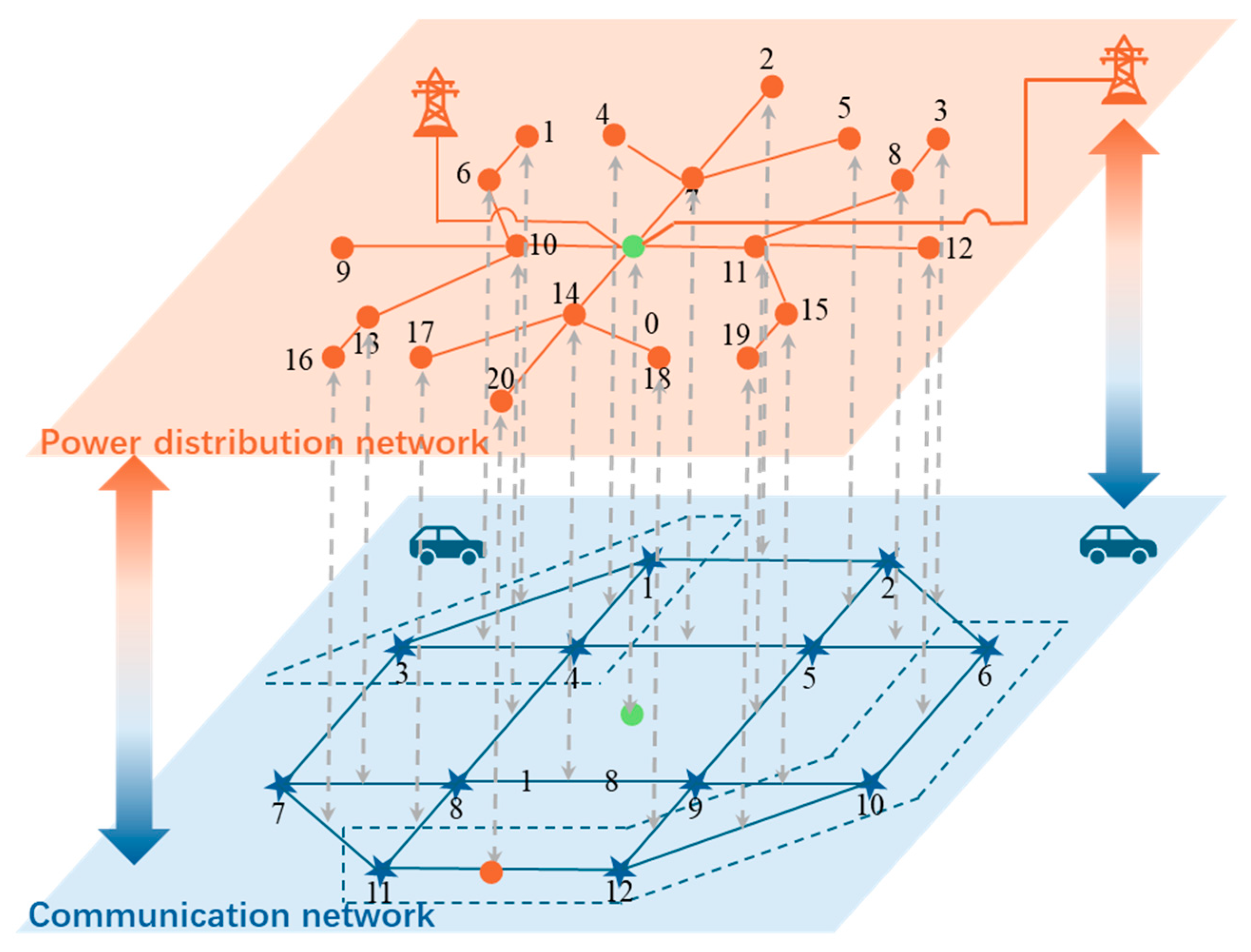
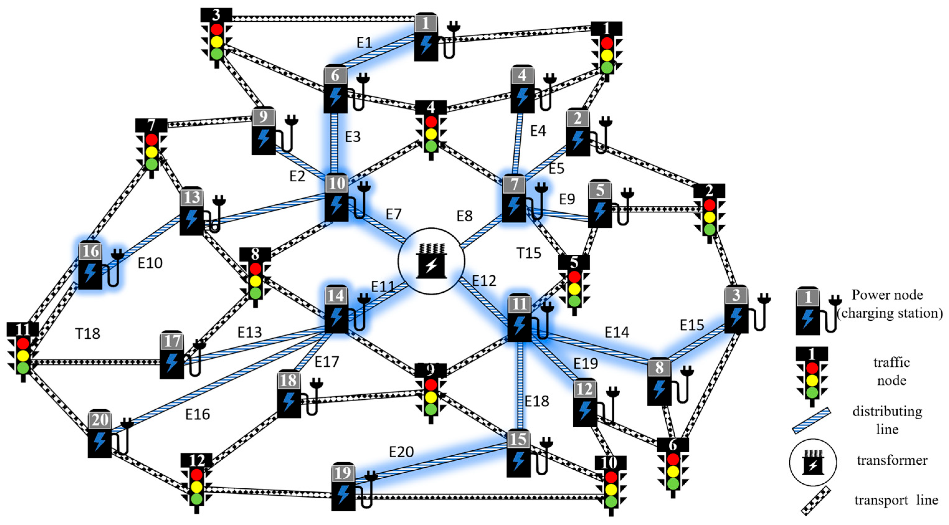
This study takes a city in the United States as an example. A coupled-system test case, shown in Figure 1, is adopted. The distribution system consists of one slack bus and 20 charging-station nodes. The transportation system consists of 12 traffic nodes, namely intersections, and 20 roads. All simulations are conducted on the Python 3.1 platform. The key economic and technical parameters of the model are set as follows.
When the electricity load of a charging station exceeds 60% of the node capacity, the station reduces its power supply to relieve load pressure. The load penalty coefficient for user compensation is set to 200 USD/(MW·h). When the load exceeds 80% of the node capacity, the charging station gradually disconnects part of the power supply to reduce load pressure. The load penalty coefficient for user compensation is then increased to 400 USD/(MW·h). The traffic delay cost of each vehicle is set to 1.5 USD/min. The EV penetration rate on each road is set to 60%. The average charging power of each vehicle is set to 0.05 MW.
The initial capacity limit of each power line is set to 250 MW. Considering that power lines require underground cabling, the expansion cost is set to 2 million USD. The corresponding capacity gain is 20%. The initial capacity limits of high-capacity power source nodes P1, P3, P5, P12, and P18 are set to 1200 MW. Their expansion cost is set to 4 million USD, and their capacity increases by 15% after expansion. The remaining power source nodes are regarded as regular power source nodes. Their initial capacity limits range from 600 to 800 MW. Their expansion cost is set to USD 5 million, and the corresponding capacity gain is 40%. The traffic capacity limit of each road is set to 600 vehicles/h. The road expansion cost is set to 1.5 million USD, and the capacity increases by 40% after expansion.

4.2. Validation of the Effectiveness and Superiority of the Prediction Algorithm Considering Scenario Labels

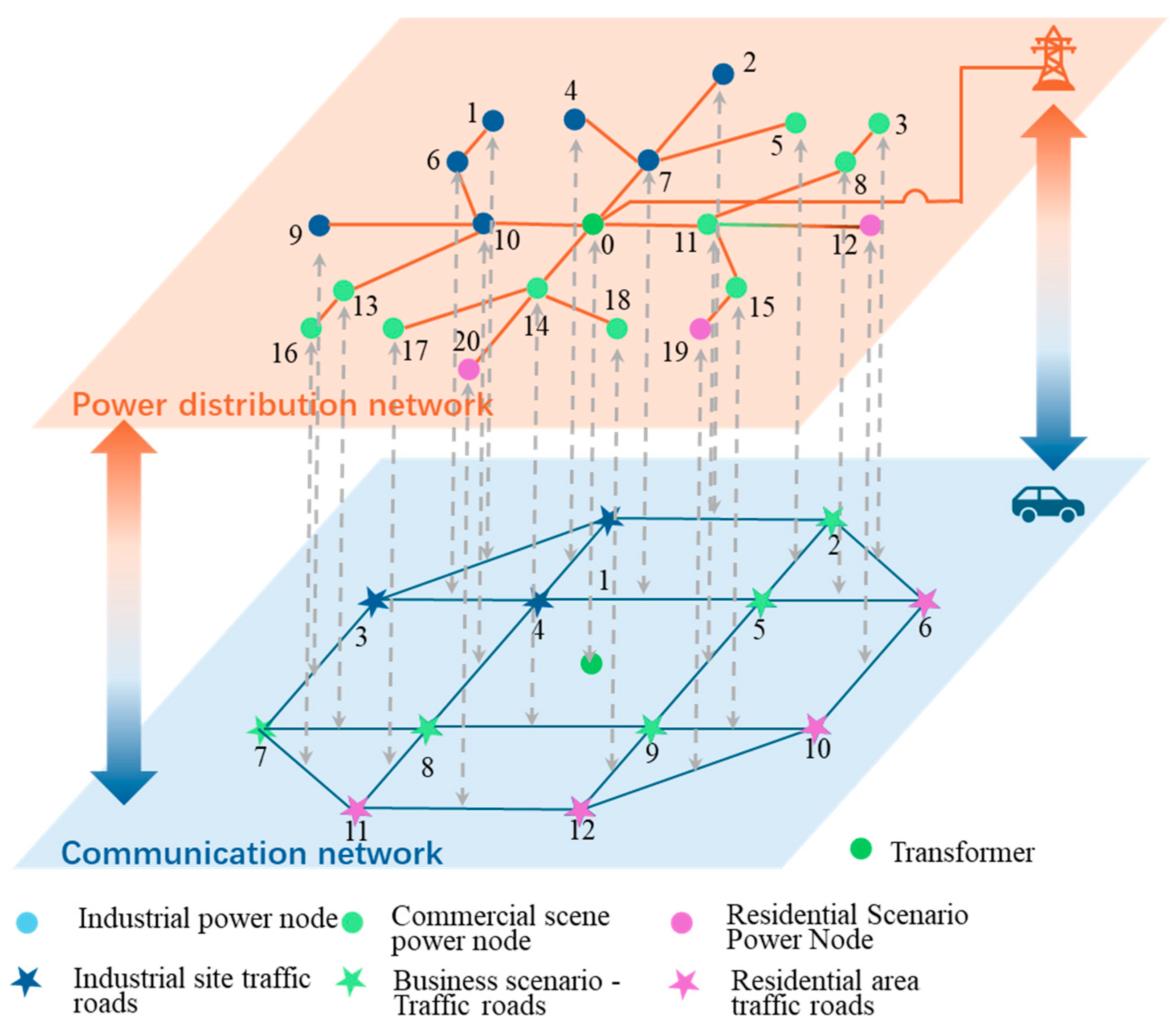
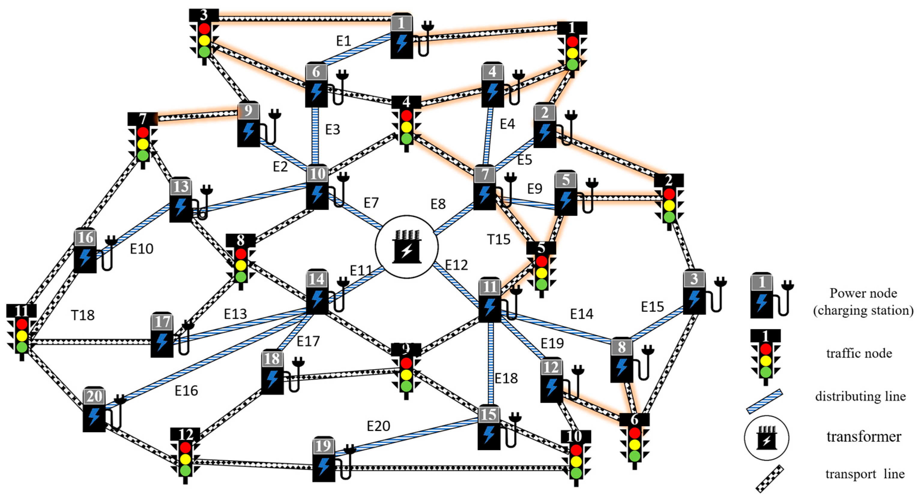
To verify the necessity of introducing scenario features and the superiority of the proposed hybrid algorithm in load and traffic flow interval forecasting, the automatic adaptive density-based clustering method proposed above is first adopted. This method identifies the spatiotemporal behavioral features of power-node loads and traffic flows on road segments. The scenario labels of different objects are then obtained. The power–transportation network diagrams after scenario classification are shown in Figure 2. The scenario labels and historical data are used as model inputs. Under the same conditions, the following comparison methods are established for evaluation.
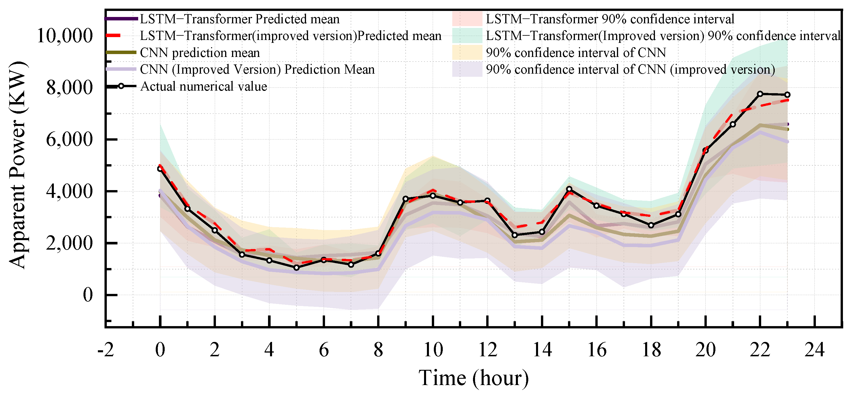
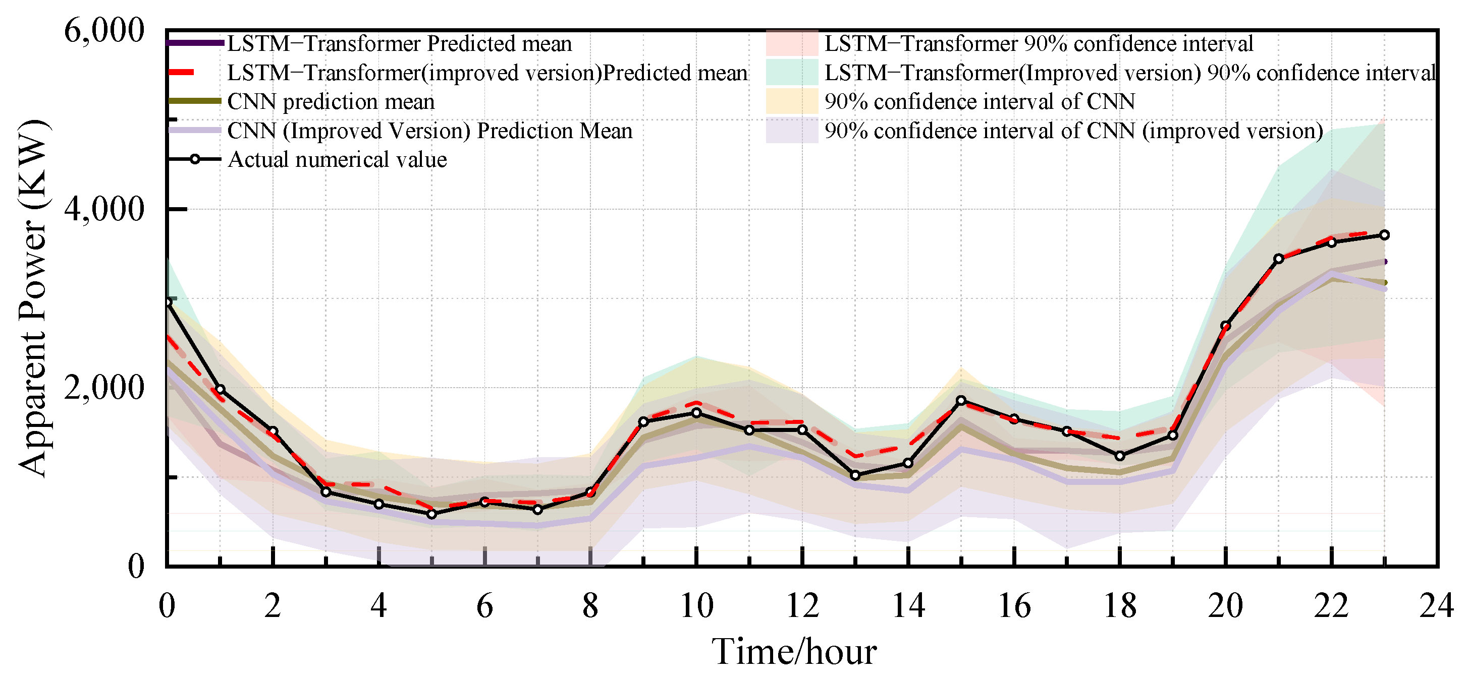
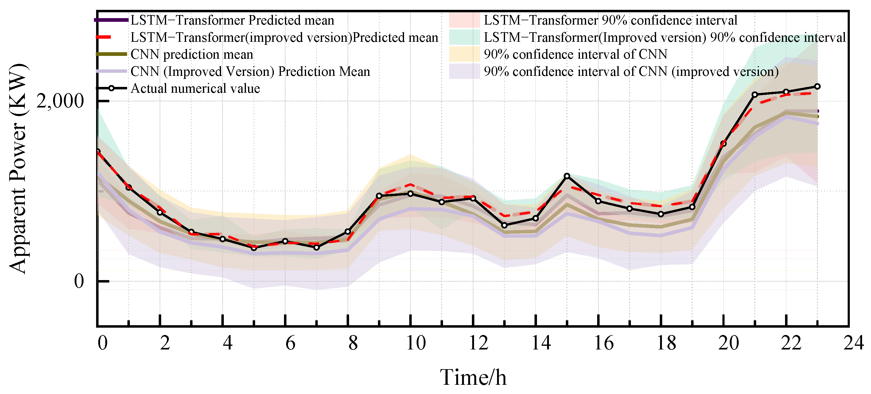
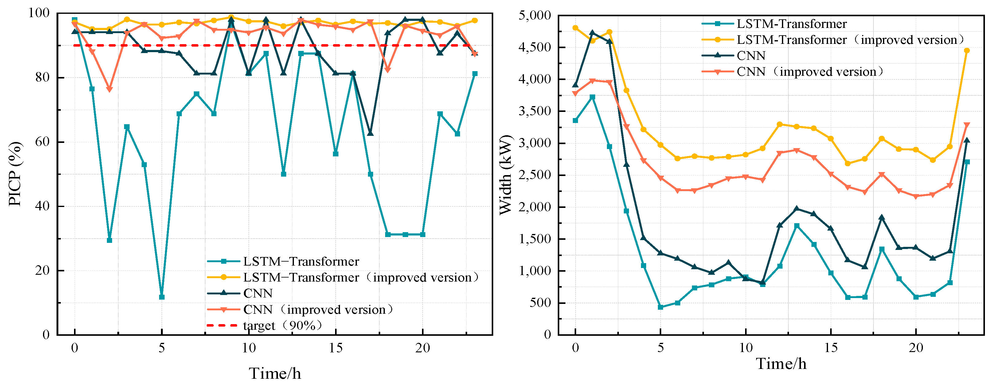
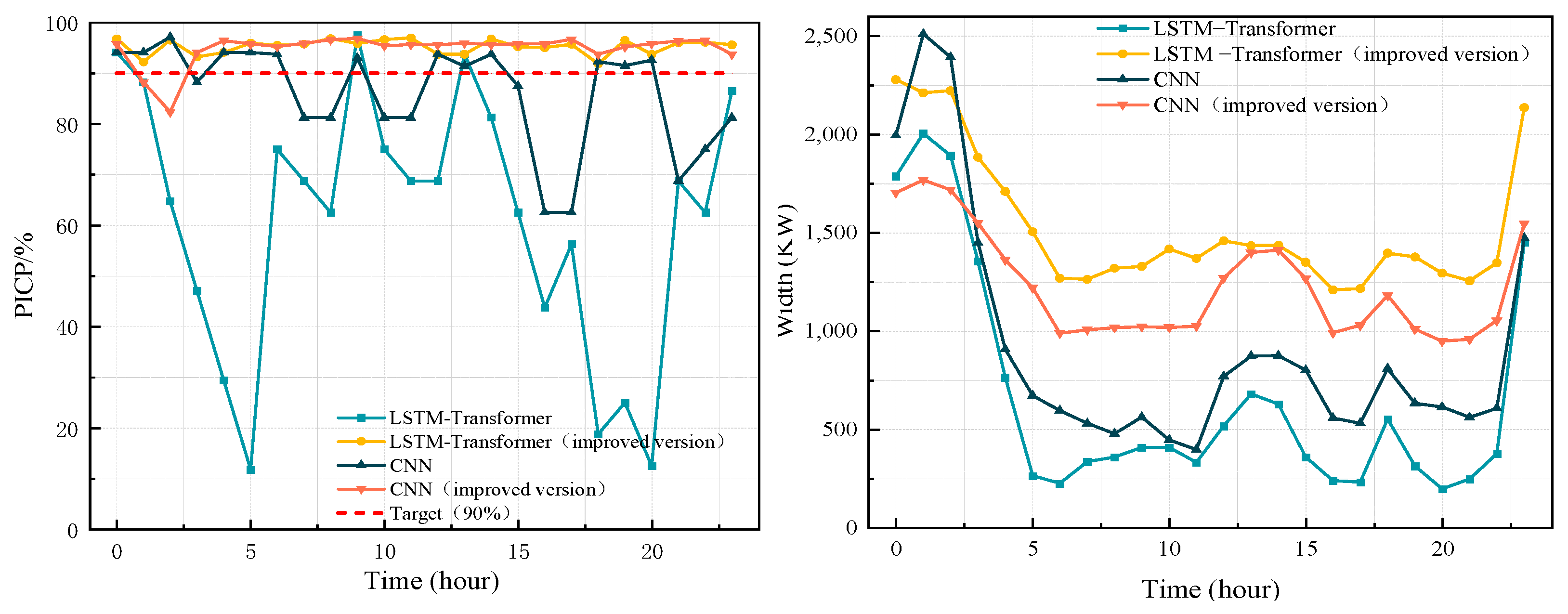
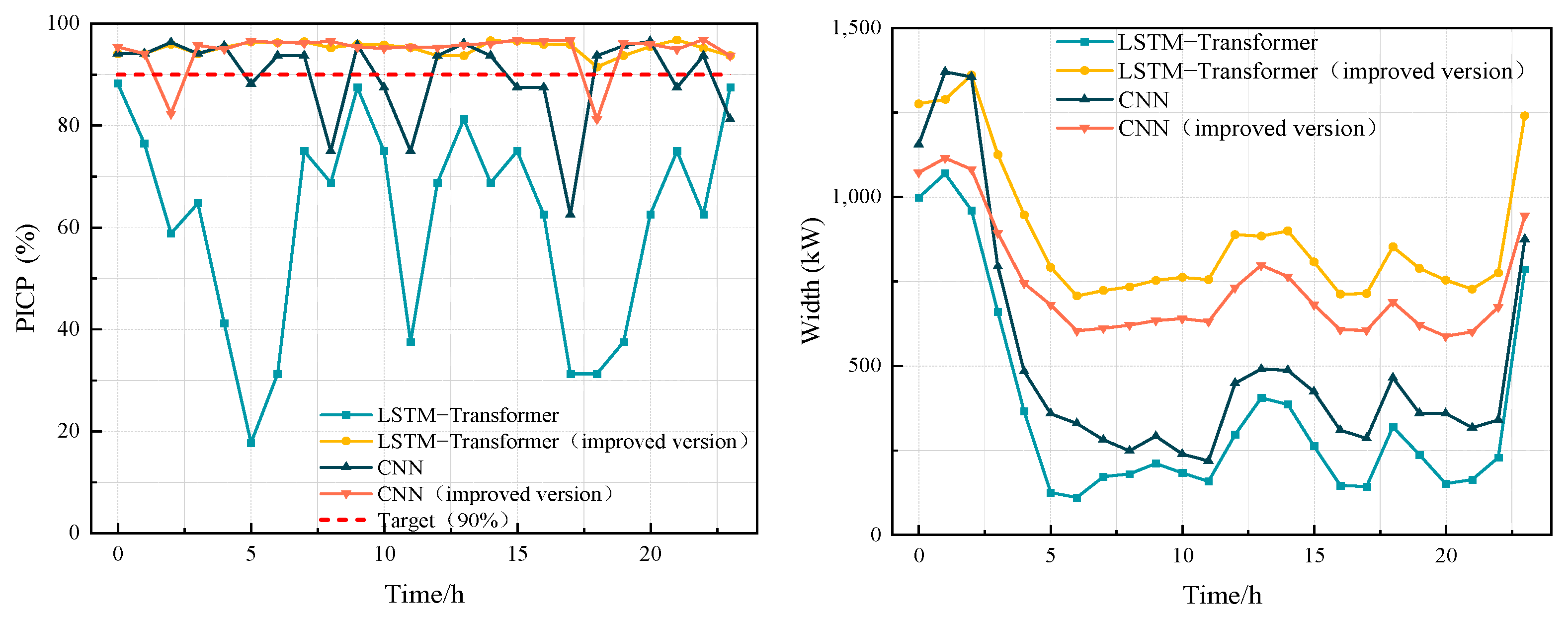
The comparison of weekday and non-weekday forecasting performance based on reliability and interval width is shown in Figure 3, Figure 4 and Figure 5.
As shown in Figure 6, Figure 7 and Figure 8, the LSTM–Transformer and CNN models are tested without scenario labels. Because scenario-specific features are unavailable, neither model can perceive load characteristics across scenarios in advance. Therefore, both models show poor forecasting accuracy. Their PICP values rarely reach 90%, and their RMSW values are relatively low. After scenario labels are introduced, the LSTM–Transformer model shows more stable performance. By contrast, CNN performs poorly at typical industrial node 7, residential node 12, and commercial node 17. At these nodes, PICP falls below 90% two, one, and two times, respectively. Its RMSW values are also unsatisfactory. This occurs because CNN mainly extracts local features through convolution kernels. It has limited ability to model global temporal dependencies and fuse label information. The LSTM–Transformer model combines LSTM-based temporal modeling with the attention mechanism. Thus, it captures complex load fluctuations under different scenarios more effectively.
4.3. Validation of the Solution Method

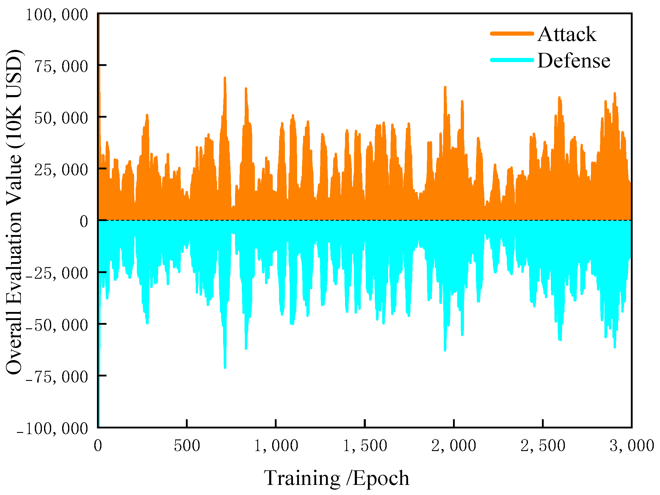
To validate the solution method, the ARL convergence curves are experimentally analyzed. Figure 9 shows the trajectory and convergence of the system evaluation value under adverse conditions. The defender minimizes this value, whereas the attacker maximizes it.
As shown in Figure 9, the defender dynamically adjusts investments in power nodes, lines, and roads. It minimizes system-wide operating losses under adverse scenarios. These losses include load shedding and traffic delays. This objective is balanced against total investment costs. The attacker targets power nodes most likely to become overloaded. It also targets roads most susceptible to congestion. Within the disturbance budget, it maximizes load-shedding and traffic-delay costs. This pressure may force the defender to increase investment. Through repeated interaction, both agents seek an optimal trade-off.
As training progresses, the attacker gradually increases the attack intensity. Consequently, the system evaluation value rises during some training stages. Meanwhile, the defender continuously learns and adapts to the attack strategy. Its response capability therefore improves throughout training. The system evaluation value under the attacker’s policy then gradually declines. Eventually, both agents reach a stable state through repeated interaction and gradually converge.
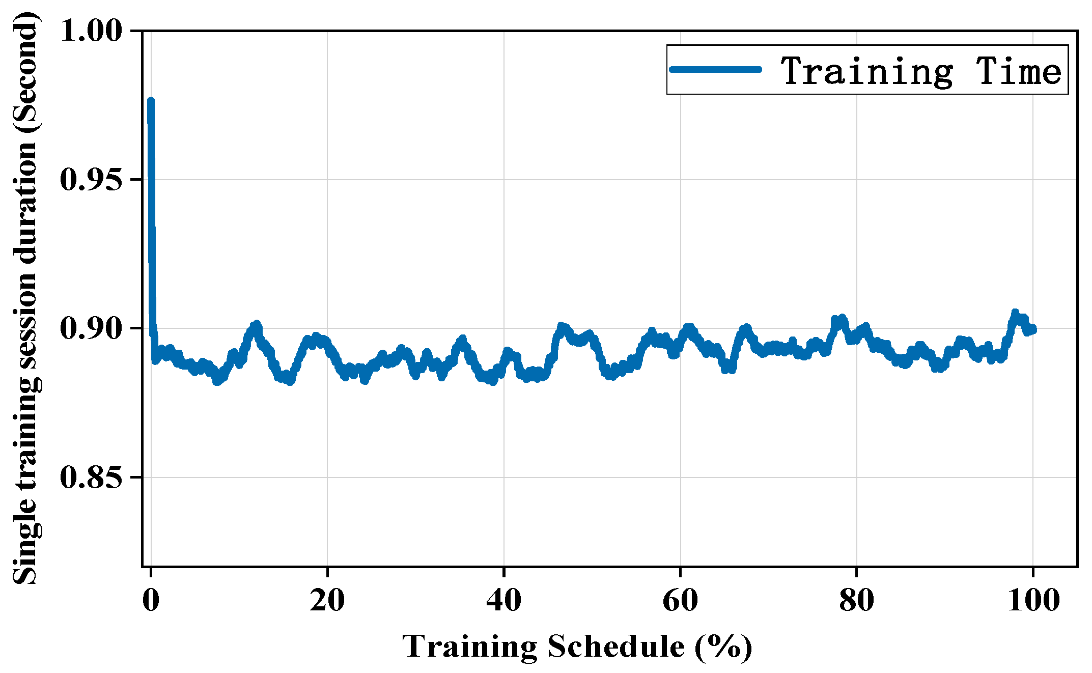
The proposed ARL is further evaluated for training efficiency. Its total training time and time complexity are analyzed in Figure 10.
As shown in Figure 10, the initial training rounds require more computation. The computational graph and operator execution paths must first be constructed. Relevant numerical variables must also be initialized. These initialization steps increase the training time. Once training stabilizes, the time per training round decreases markedly.
As training progresses, the attack intensity gradually increases. The training time therefore rises slowly. However, the iterations of dynamic user equilibrium (DUE) are limited. An attack-action pruning mechanism is also applied. These measures restrict the growth in computational cost.

4.4. Comparison and Superiority Analysis of Planning Methods

Traditional distribution network planning often relies on typical-day data. Therefore, the data used for planning are usually static. This practice ignores spatial and temporal differences in load variations. It can easily disconnect planning schemes from actual operational requirements. To address this problem, the preceding sections first classify load features using automatic adaptive density-based clustering. Then, a hybrid algorithm is used to predict confidence intervals for typical-day data. Conventional solution algorithms are not well suited to confidence-interval optimization problems.
This study adopts an adversarial reinforcement learning method to solve the proposed planning problem. The defender agent first generates an initial grid investment scheme. The attacker then generates probability-consistent perturbations within the data confidence intervals. These perturbations are imposed to conduct stress testing. Finally, the model evaluates the planning performance under perturbations. The resulting rewards and penalties are fed back to both the defender and attacker. This feedback drives both agents to optimize their strategies alternately over multiple iterations. The process continues until the strategies converge toward a Nash equilibrium. A robust planning scheme is then obtained. It balances economic performance and all-weather adaptability.
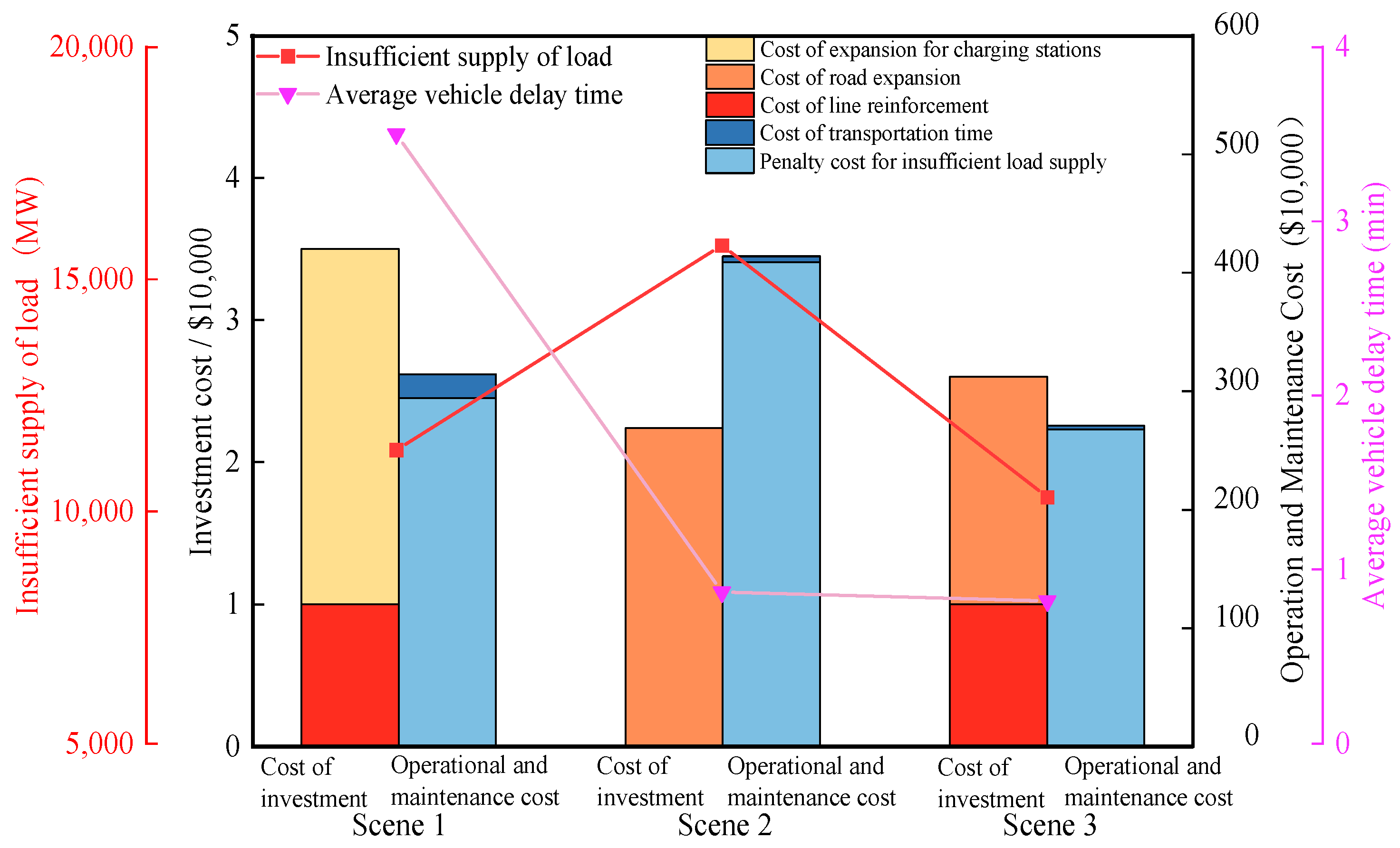
To verify the effectiveness of the resilience enhancement strategy, three scenarios are designed for simulation analysis. The calculation results are shown in Figure 9.
Scenario 1: Only investment in the power network is considered.
Scenario 2: Only investment in the transportation network is considered.
Scenario 3: Joint investment in the coupled power–transportation network is considered.
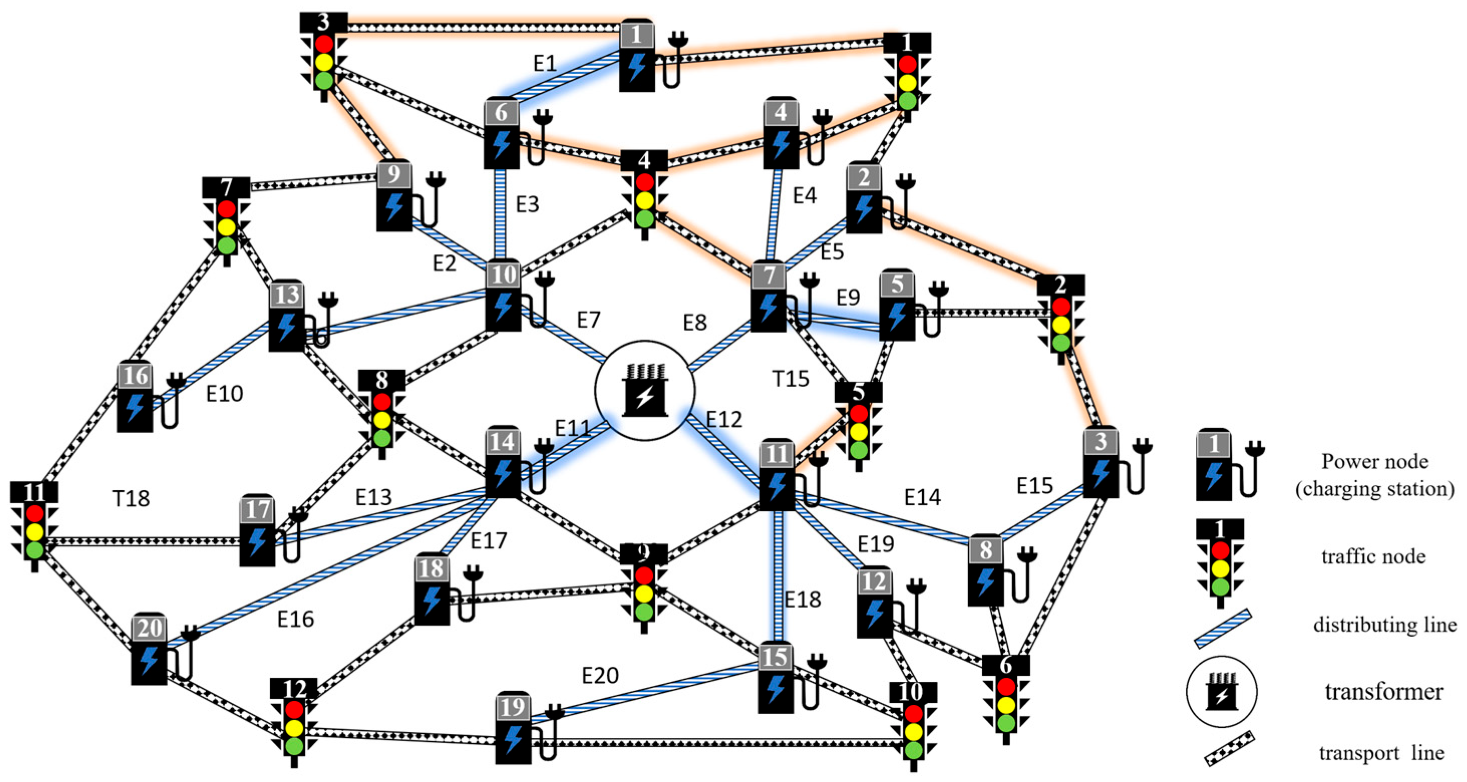
As shown in Figure 11, the investment costs of Scenarios 1, 2, and 3 are USD 43.00 million, USD 22.40 million, and USD 26.00 million, respectively. The corresponding operation and maintenance costs under adverse conditions are USD 3.14224 million, USD 4.1397 million, and USD 2.72424 million, respectively. This is because Scenario 3 considers the coupling between the power and transportation networks during investment planning. By investing in transportation links, EVs are guided to charging stations with lower loading rates. These stations may be farther away from the EVs. This strategy protects some charging stations and power lines from overload. In addition, investment in power lines and charging stations affects EV charging choices. EVs are encouraged to choose smoother traffic routes, even if these routes require detours or longer travel distances. This reduces congestion on some busy transportation links. Thus, Scenario 3 improves the utilization of coupled network resources. According to the reported total expenditure, its total cost is reduced by USD 418,000 compared with Scenario 1. It is also reduced by USD 1.41546 million compared with Scenario 2. Therefore, Scenario 3 maximizes investment efficiency. The investment schemes under different scenarios are shown in Figure 12, Figure 13 and Figure 14.
Analysis of Figure 12, Figure 13 and Figure 14 shows that Scenario 1 lacks transportation-side guidance measures. As a result, EVs charge in an uncontrolled manner. Constrained by uncontrolled EV charging, the planner has to invest in nine power lines and expand five power nodes. All overload-prone power lines and nodes are expanded. Additional investment is allocated to some core areas to attract part of the EV charging demand. Under adverse conditions, transportation corridors are likely to experience widespread congestion. Therefore, the investment efficiency is relatively low.
Figure 15 shows that Scenario 3 selects five power lines and 13 transportation links for investment. Joint investment activates the power–transportation coupling mechanism. This mechanism guides EV travel and charging decisions. Selectively widening links toward lightly loaded power nodes encourages EV drivers to reroute for charging. Investments in highly loaded power nodes and lines also strengthen grid resilience. Even under extreme conditions, bounded rationality may induce suboptimal and non-cooperative driving behavior. The proposed game model anticipates these worst-case behavioral disturbances during adversarial training. It then incorporates them into the learned strategy. Thus, the coordinated investment scheme remains robust even when users do not fully comply. These results show that coordinated power–transportation planning markedly reduces losses under adverse conditions.

4.5. Sensitivity Analysis and Robustness Verification

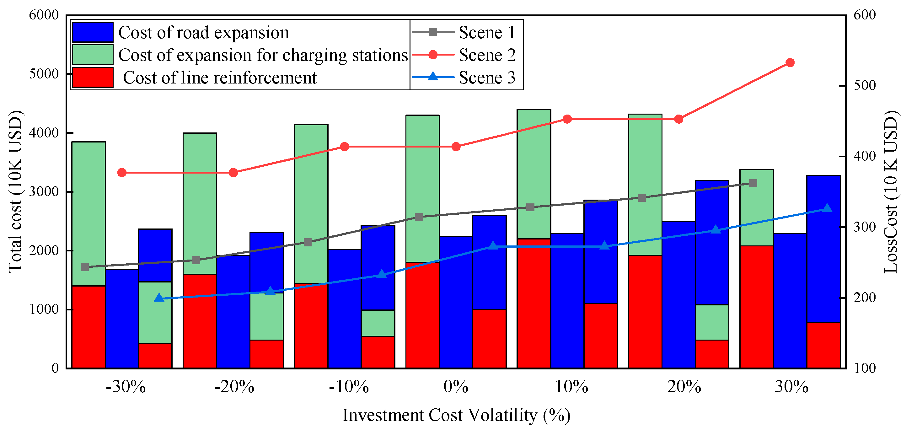
The preceding analysis demonstrates the economic benefits of coordinated planning. Further sensitivity analyses validate the proposed ARL framework as a statistically robust decision tool. They also assess whether the framework avoids overfitting to a single dataset. The analyses examine investment-cost variations and regional EV penetration levels. Their effects on the planning scheme are evaluated. Figure 15 shows the results under varying infrastructure investment costs. It compares investment costs and adverse-weather operational losses across all scenarios.
Figure 15 shows that higher investment costs generally reduce the investment scale across all scenarios. When costs decline, more projects are selected to reduce adverse-weather operating losses. For Scenario 2, 14 roads are expanded at the baseline cost. A 10% cost increase reduces this number to 13. At 20%, the number remains unchanged due to the trade-off between marginal investment costs and loss risks. At 30%, cost pressure reduces the number to 11. Meanwhile, adverse-weather operating losses rise markedly.
Scenario 3 demonstrates the flexibility of coupled power–transportation investment. As investment costs rise, Scenario 3 prioritizes transportation assets with slower cost growth. This adjustment helps preserve system resilience. At the baseline cost, five power lines and ten roads are selected. The plan remains unchanged after a 10% cost increase. After a 20% increase, the plan includes 1 charging station, 2 power lines, and 11 roads. After a 30% increase, the plan selects 3 power lines and 12 roads. Compared with Scenarios 1 and 2, Scenario 3 has lower operating losses. Its loss growth rate is also lower. These results demonstrate the framework’s robustness to cost variations and its superior decision performance.
The impact of abrupt local policy changes on planning decisions is examined. In practice, some cities restrict internal-combustion-engine vehicles in central business districts [29]. Such policies can substantially increase EV penetration in selected urban areas. This creates spatial differences in regional EV penetration. Figure 16 presents the sensitivity analysis of these policy-induced penetration shifts.
At regional EV penetration shifts of 0–10%, charging demand concentrates in several hotspots. This pattern enables targeted investment in nearby power and transportation infrastructure. Consequently, the overall number of planned projects declines across all scenarios. For Scenario 3, the initial plan includes five power lines and ten roads. The total investment is $26 million. The plan gradually contracts two power lines, two charging stations, and five roads. The total investment then falls to USD 22 million. Adverse-weather operating losses also decline from USD 2.72 million to USD 2.19 million. These results show that targeted expansion reduces both investment costs and operating losses at modest concentration level.
When the concentration level rises from 10% to 30%, expansion resources in hotspot areas gradually become saturated. Investment therefore spreads outward, while project counts and losses increase rapidly. At this stage, the limitations of single-network planning become evident. Scenarios 1 and 2 invest only in power or transportation infrastructure. Once local capacity is saturated, these schemes cannot expand effectively. Congestion and other adverse-weather losses then rise sharply with EV penetration. Scenario 3 does not simply concentrate investment in high-penetration areas. Instead, coordinated power–transportation planning differentiates charging-station and road deployment. This design redirects vehicle flows and delays congestion growth. Scenario 3 reaches USD 3.29 million in adverse-weather operating losses. This remains below the USD 3.73 million and USD 6.51 million in Scenarios 1 and 2. These results demonstrate stronger decision robustness under changing urban EV penetration patterns.
5. Conclusions

This study addresses spatiotemporal load fluctuations and extreme disturbance risks in coupled power–transportation systems under large-scale electric vehicle integration. A resilience planning method based on scenario-feature identification and adversarial reinforcement learning is proposed. First, an automatic density-based clustering method is used to identify the operational characteristics of power nodes, distribution lines, and transportation links. Typical scenarios are then classified according to holiday and non-holiday conditions, as well as industrial, commercial, and residential areas. Then, scenario labels are introduced into the LSTM–Transformer model to achieve interval forecasting of power load and traffic flow. Finally, a resilience planning model for the coupled power–transportation system is constructed by integrating metrics such as node loading rate, line loading rate, and traffic delay time. Case studies show that the proposed method effectively improves the planning performance of the coupled power–transportation system. After scenario labels are introduced, the PICP values of the LSTM–Transformer interval forecasting model generally satisfy the 0.9 confidence-level requirement. In the planning results, the operation and maintenance cost of the joint power–transportation investment scenario under adverse conditions is USD 2.72424 million. This value is lower than USD 3.14224 million for the power network-only investment scenario and USD 4.1397 million for the transportation network-only investment scenario. These results indicate that coordinated planning reduces operational losses under extreme scenarios and improves overall system resilience.

Author Contributions

Methodology, S.Y.; Software, Q.D.; Validation, B.L. and J.Q.; Formal analysis, S.Y. and B.L.; Investigation, Y.W. and Q.D.; Data curation, Y.W. and J.Q.; Writing–original draft, S.Y.; Writing–review & editing, J.G.; Visualization, Y.W. and B.L.; Supervision, Y.H.; Project administration, Y.H.; Funding acquisition, Y.H. All authors have read and agreed to the published version of the manuscript.

Funding

This research was funded by Guangdong Power Grid Co., LTD (grant numbers 0300002023030103GH00050, 0319002024030103D200225, and 03000020250302010300039) and the Electric Power Research Institute of State Grid Hebei Electric Power Co., Ltd. (grant number SGHEDK00JSJS2400157). And The APC was funded by Guangdong Power Grid Co., Ltd. (grant number 03000020250302010300039).

Data Availability Statement

The data presented in this study are available on request from the corresponding author. The data are not publicly available due to [privacy].

Conflicts of Interest

Authors Shuiping Yi, Yuxue Wang and Bo Li was employed by the company Guangdong Power Grid Co., Ltd. Author Qiaoxu Dai was employed by the company Zhanjiang Power Supply Bureau of Guangdong Power Grid Co., Ltd. Author Junyuan Qu was employed by the company Jiangmen Power Supply Bureau of Guangdong Power Grid Co., Ltd. Author Jian Guan was employed by the company Shantou Power Supply Bureau of Guangdong Power Grid Co., Ltd. The remaining authors declare that the research was conducted in the absence of any commercial or financial relationships that could be construed as a potential conflict of interest.

References

  1. Han, X.; Wang, S.; Yu, J.; Wang, P.; Li, X. Design of PUF based on a Cr2O3-SnO2 gas sensor for Internet of Things security. Measurement 2026, 276, 121395. [Google Scholar] [CrossRef] [Scilit]
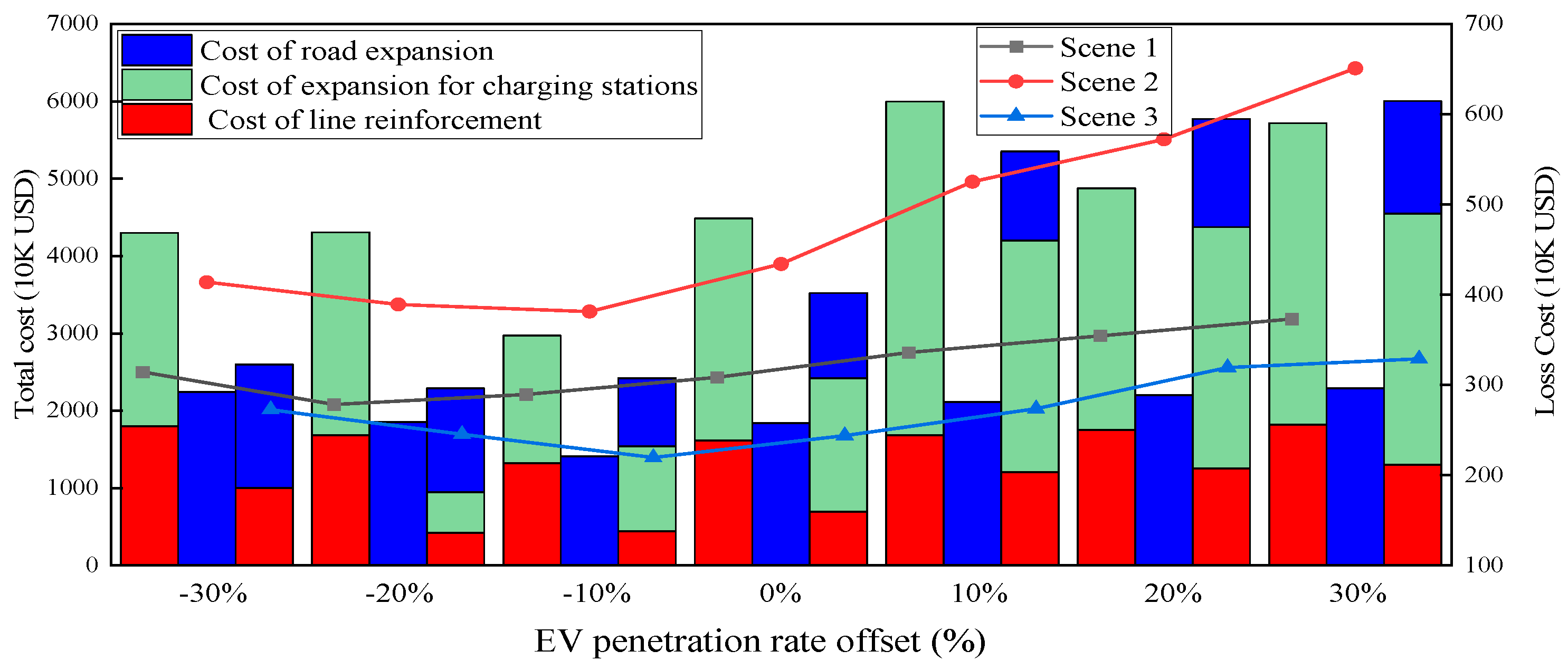
  2. Wang, S.; Zhang, X.; Wang, P.; Li, X. Design of Magnetic Sensor Array-Based PUFs for IoT Security. IEEE Trans. Instrum. Meas. 2026; early access. [CrossRef] [Scilit]
  3. Wang, W.; Han, C.; Xu, D.; Sun, H.; Sun, R.; Qin, F.; Wu, H.; Sun, Z. Anisotropic surface inspired by reed leaves for water droplet energy harvesting. Chem. Eng. J. 2026, 529, 172661. [Google Scholar] [CrossRef] [Scilit]
  4. Zhu, G.; Zhang, S.; Deng, Z.; Wang, J.; Li, Y.; Dong, J.; Bauer, P. Extended hybrid modulation for multi-stage constant-current wireless ev charging. IEEE Trans. Power Electron. 2025, 40, 10095–10110. [Google Scholar] [CrossRef] [Scilit]
  5. Zhu, G.; Dong, J.; Grazian, F.; Bauer, P. A hybrid modulation scheme for efficiency optimization and ripple reduction in secondary-side controlled wireless power transfer systems. IEEE Trans. Transp. Electrif. 2024, 11, 6840–6853. [Google Scholar] [CrossRef] [Scilit]
  6. Srivastava, A.; Manas, M.; Dubey, R.K. Integration of power systems with electric vehicles: A comprehensive review of impact on power quality and relevant enhancements. Electr. Power Syst. Res. 2024, 234, 110572. [Google Scholar] [CrossRef] [Scilit]
  7. Powell, S.; Cezar, G.V.; Rajagopal, R. Scalable probabilistic estimates of electric vehicle charging given observed driver behavior. Appl. Energy 2022, 309, 118382. [Google Scholar] [CrossRef] [Scilit]
  8. Wang, S.; Chen, A.; Wang, P.; Zhuge, C. Predicting electric vehicle charging demand using a heterogeneous spatio-temporal graph convolutional network. Transp. Res. Part C Emerg. Technol. 2023, 153, 104205. [Google Scholar] [CrossRef] [Scilit]
  9. Czétány, L.; Vámos, V.; Horváth, M.; Szalay, Z.; Mota-Babiloni, A.; Deme-Bélafi, Z.; Csoknyai, T. Development of electricity consumption profiles of residential buildings based on smart meter data clustering. Energy Build. 2021, 252, 111376. [Google Scholar] [CrossRef] [Scilit]
  10. Komatsu, H.; Kimura, O. Customer segmentation based on smart meter data analytics: Behavioral similarities with manual categorization for building types. Energy Build. 2023, 283, 112831. [Google Scholar] [CrossRef] [Scilit]
  11. Pentsos, V.; Tragoudas, S.; Wibbenmeyer, J.; Khdeer, N. A hybrid LSTM-Transformer model for power load forecasting. IEEE Trans. Smart Grid 2025, 16, 2624–2634. [Google Scholar] [CrossRef] [Scilit]
  12. Hu, J.; Hu, W.; Cao, D.; Sun, X.; Chen, J.; Huang, Y.; Chen, Z.; Blaabjerg, F. Probabilistic net load forecasting based on transformer network and Gaussian process-enabled residual modeling learning method. Renew. Energy 2024, 225, 120253. [Google Scholar] [CrossRef] [Scilit]
  13. Wang, Y.; Zhou, B.; Xu, Y.; Chung, C.Y.; Yang, Y.; Yuan, Z.; Hu, C. Spatio-Temporal Power Outage Risk Prediction for Interdependent Urban Electricity and Drainage Networks Under Rainstorm Disasters. IEEE Trans. Smart Grid 2026, 17, 2888–2902. [Google Scholar] [CrossRef] [Scilit]
  14. Guo, S.; Zhou, B.; Chung, C.Y.; Bu, S.; Hua, Z.; Liu, J.; Hu, W. Hierarchical Aggregation-Embedded Emergency Scheduling of Coupled Electricity-Watershed Networks With Heterogeneous Flexibility Resources Under Extreme Drought Events. IEEE Trans. Sustain. Energy 2025, 17, 1894–1908. [Google Scholar] [CrossRef] [Scilit]
  15. Zhou, Z.; Moura, S.J.; Zhang, H.; Zhang, X.; Guo, Q.; Sun, H. Power-traffic network equilibrium incorporating behavioral theory: A potential game perspective. Appl. Energy 2021, 289, 116703. [Google Scholar] [CrossRef] [Scilit]
  16. Liang, Z.; Qian, T.; Korkali, M.; Glatt, R.; Hu, Q. A Vehicle-to-Grid planning framework incorporating electric vehicle user equilibrium and distribution network flexibility enhancement. Appl. Energy 2024, 376, 124231. [Google Scholar] [CrossRef] [Scilit]
  17. Shi, H.; Xiong, H.; Gan, W.; Lin, Y.; Guo, C. Fully distributed planning method for coordinated distribution and urban transportation networks considering three-phase unbalance mitigation. Appl. Energy 2025, 377, 124449. [Google Scholar] [CrossRef] [Scilit]
  18. Guo, W.; Liu, G.; Zhou, Z.; Wang, J.; Tang, Y.; Wang, M. Robust training in multiagent deep reinforcement learning against optimal adversary. IEEE Trans. Syst. Man Cybern. Syst. 2025, 55, 4957–4968. [Google Scholar] [CrossRef] [Scilit]
  19. Hua, Z.; Zhou, B.; Chan, K.W.; Zhang, C.; Cao, Y.; Wang, P.; Xia, M. A progressive polyhedral approximation method for nonlinear PDE-constrained electricity-water nexus dispatch. IEEE Trans. Smart Grid 2025, 16, 2703–2706. [Google Scholar] [CrossRef] [Scilit]
  20. Gao, W.; Deng, C.; Jiang, Y.; Jiang, Z.-P. Resilient reinforcement learning and robust output regulation under denial-of-service attacks. Automatica 2022, 142, 110366. [Google Scholar] [CrossRef] [Scilit]
  21. Zhou, Z.; Liu, G.; Guo, W.; Zhou, M. Adversarial attacks on multiagent deep reinforcement learning models in continuous action space. IEEE Trans. Syst. Man Cybern. Syst. 2024, 54, 7633–7646. [Google Scholar] [CrossRef] [Scilit]
  22. Ren, C.; Du, X.; Xu, Y.; Song, G.; Liu, Y.; Tan, R. Vulnerability analysis, robustness verification, and mitigation strategy for machine learning-based power system stability assessment model under adversarial examples. IEEE Trans. Smart Grid 2021, 13, 1622–1632. [Google Scholar] [CrossRef] [Scilit]
  23. Macas, M.; Wu, C.; Fuertes, W. Adversarial examples: A survey of attacks and defenses in deep learning-enabled cybersecurity systems. Expert Syst. Appl. 2024, 238, 122223. [Google Scholar] [CrossRef] [Scilit]
  24. Neufeld, A.; Sester, J. Robust Q-learning algorithm for Markov decision processes under Wasserstein uncertainty. Automatica 2024, 168, 111825. [Google Scholar] [CrossRef] [Scilit]
  25. Li, Y.; Shapiro, A. Rectangularity and Duality of Distributionally Robust Markov Decision Processes. Math. Program. 2025, 1–42. [Google Scholar] [CrossRef] [Scilit]
  26. Selim, A.; Zhao, J.; Ding, F.; Miao, F.; Park, S.-Y. Adaptive deep reinforcement learning algorithm for distribution system cyber attack defense with high penetration of DERs. IEEE Trans. Smart Grid 2023, 15, 4077–4089. [Google Scholar] [CrossRef] [Scilit]
  27. Guo, M.; Kou, P.; Tian, R.; Zhang, Y.; Liang, D. Speed Probabilistic Forecasting of Multiple Wind Turbines in WindFarm Based on Bayesian Graph Convolutional Neural Network. Trans. China Electrotech. Soc. 2025, 40, 5539–5552. [Google Scholar] [CrossRef]
  28. Yang, X.; Yun, J.; Zhou, S.; Lie, T.T.; Han, J.; Xu, X.; Wang, Q.; Ge, Z. A spatiotemporal distribution prediction model for electric vehicles charging load in transportation power coupled network. Sci. Rep. 2025, 15, 4022. [Google Scholar] [CrossRef] [Scilit]
  29. Chen, Y.; Zheng, Y.; Hu, S.; Xie, S.; Yang, Q. Optimal operation of fast charging station aggregator in uncertain electricity markets considering onsite renewable energy and bounded EV user rationality. IEEE Trans. Ind. Inform. 2024, 20, 13384–13395. [Google Scholar] [CrossRef] [Scilit]
  30. Wang, J.; Hu, H.; Nguyen, D.P.; Fisac, J.F. Magics: Adversarial RL with minimax actors guided by implicit critic stackelberg for convergent neural synthesis of robot safety. In International Workshop on the Algorithmic Foundations of Robotics; Springer Nature: Cham, Switzerland, 2024; pp. 459–480. [Google Scholar] [CrossRef] [Scilit]
Figure 1. Coupled power–Transportation Network Diagram.
Energies 19 04078 g001
Figure 2. The forecasting results of representative nodes in different scenarios.
Energies 19 04078 g002
Figure 3. Prediction Interval of Node 7.
Energies 19 04078 g003
Figure 4. Prediction Interval of Node 12.
Energies 19 04078 g004
Figure 5. Prediction Interval of Node 17.
Energies 19 04078 g005
Figure 6. Node 7 PICP RMSW.
Energies 19 04078 g006
Figure 7. Node 12 PICP RMSW.
Energies 19 04078 g007
Figure 8. Node 17 PICP RMSW.
Energies 19 04078 g008
Figure 9. Attack–defense confrontation game curve.
Energies 19 04078 g009
Figure 10. Training time complexity curve.
Energies 19 04078 g010
Figure 11. Analysis of simulation results under different scenarios.
Energies 19 04078 g011
Figure 12. Investment scheme under Scenario 1.
Energies 19 04078 g012
Figure 13. Investment scheme under Scenario 2.
Energies 19 04078 g013
Figure 14. Investment scheme under Scenario 3.
Energies 19 04078 g014
Figure 15. Sensitivity analysis of investment cost variations.
Energies 19 04078 g015
Figure 16. Sensitivity analysis of regional EV penetration shifts.
Energies 19 04078 g016
Disclaimer/Publisher’s Note: The statements, opinions and data contained in all publications are solely those of the individual author(s) and contributor(s) and not of MDPI and/or the editor(s). MDPI and/or the editor(s) disclaim responsibility for any injury to people or property resulting from any ideas, methods, instructions or products referred to in the content.