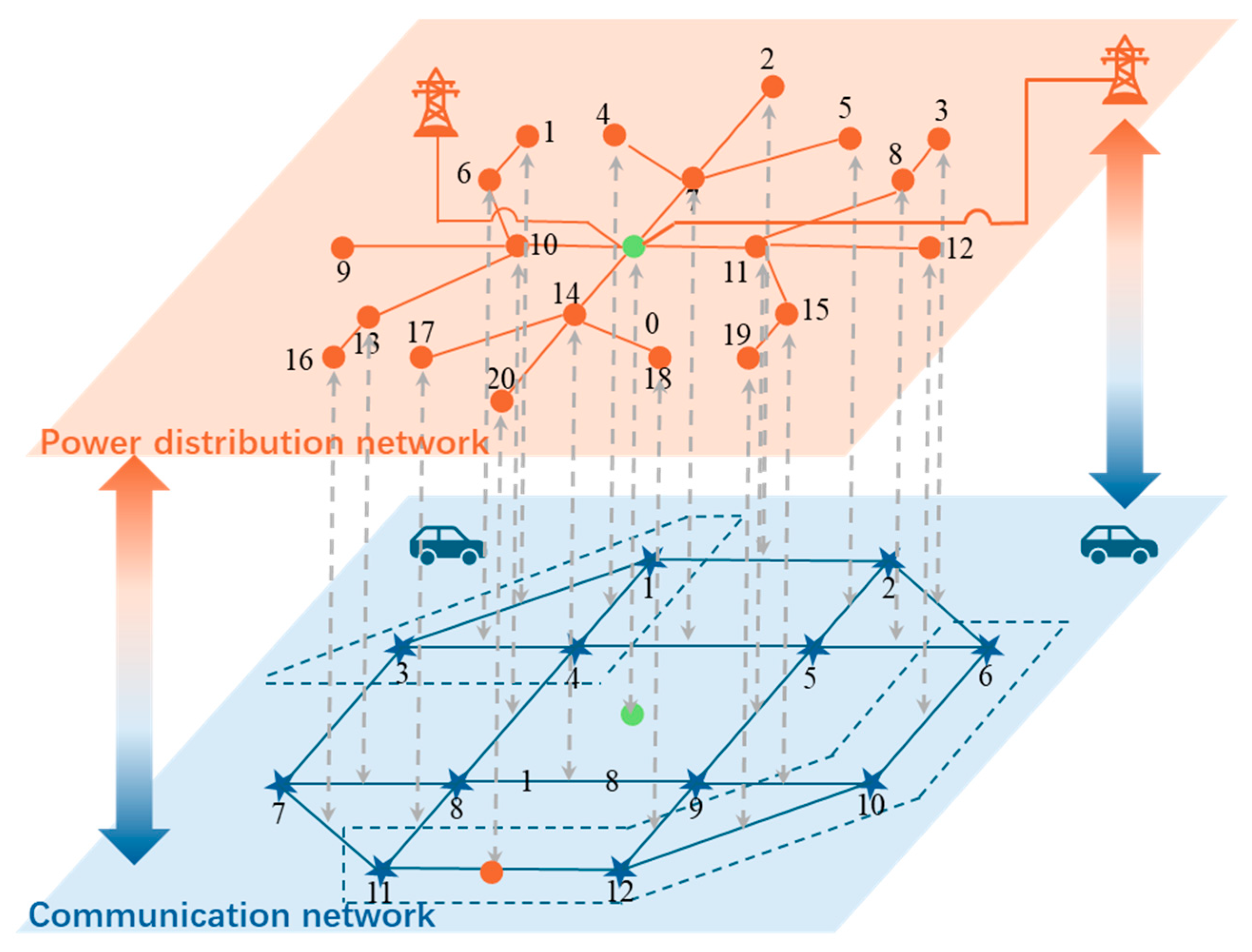
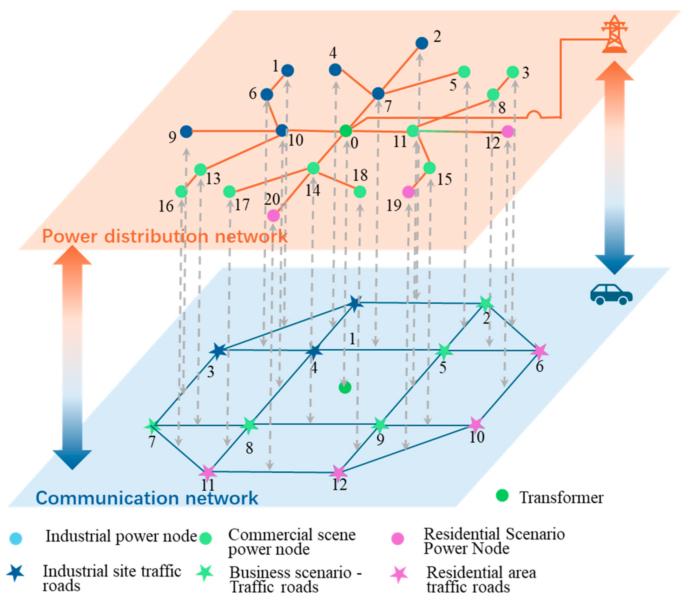
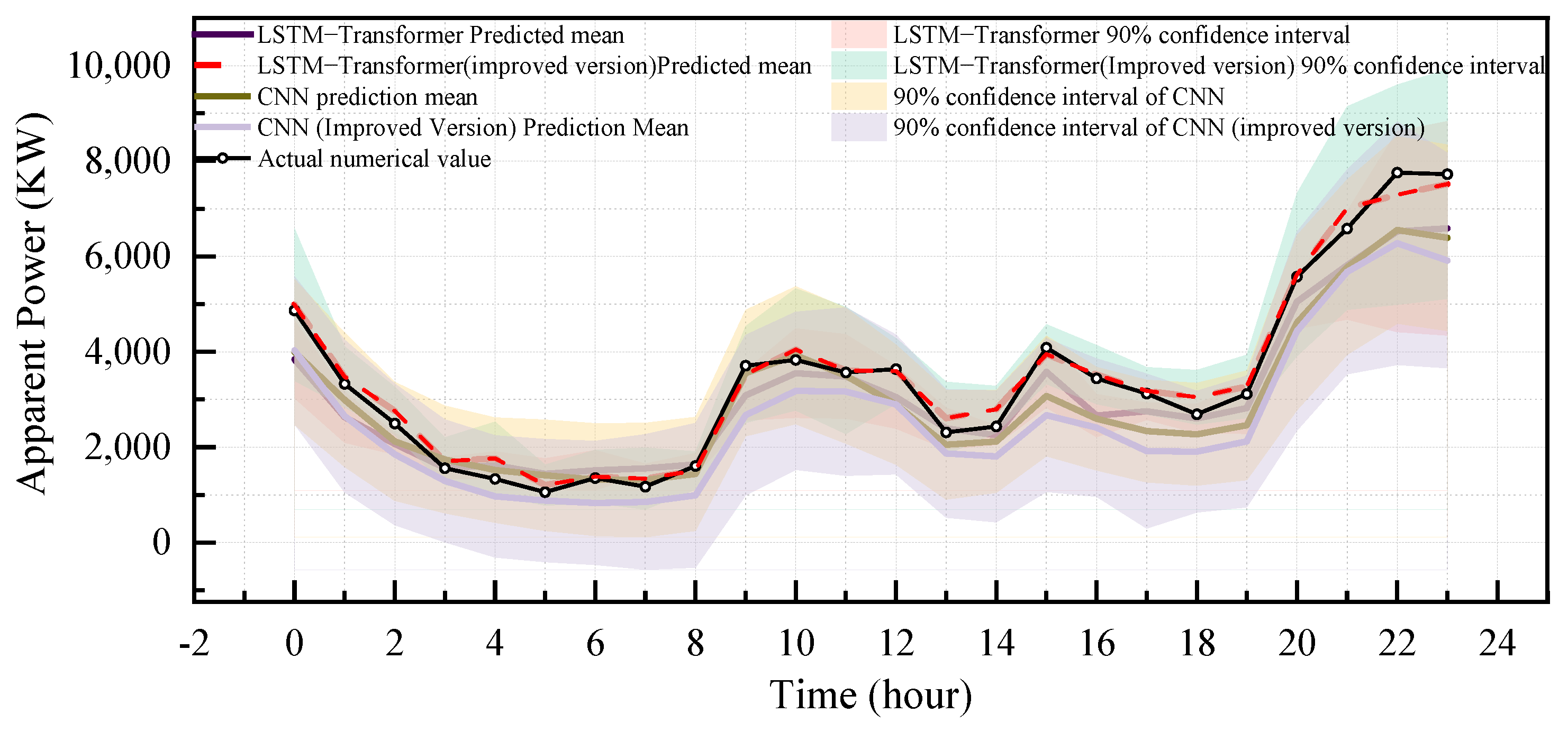
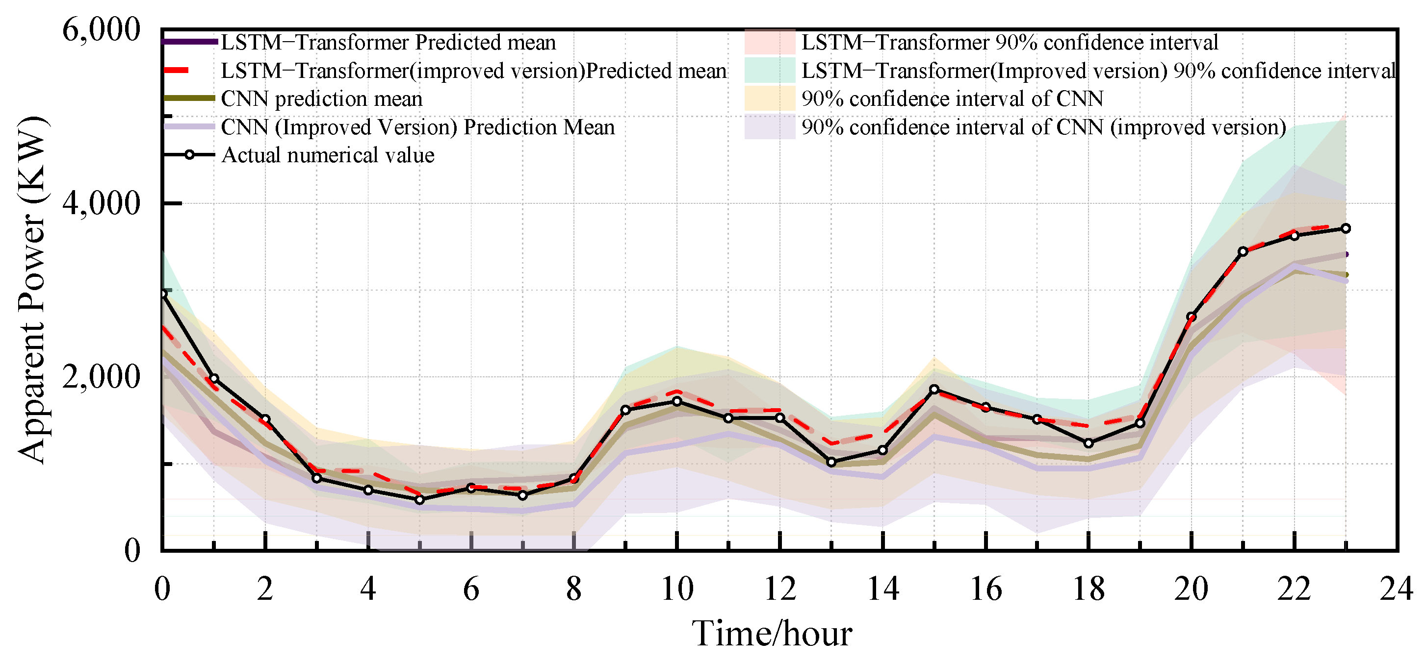
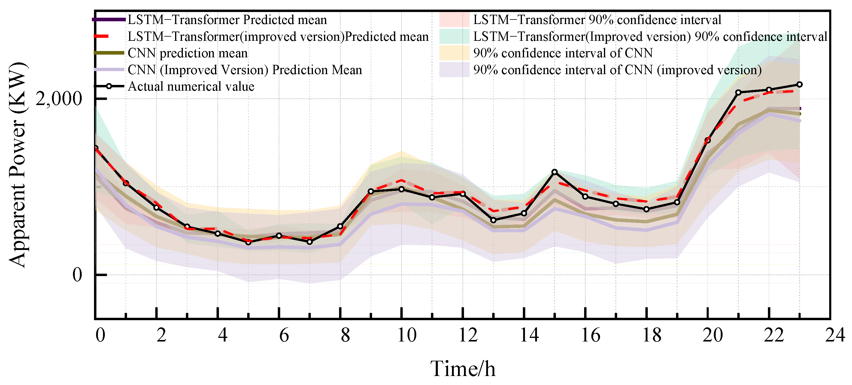
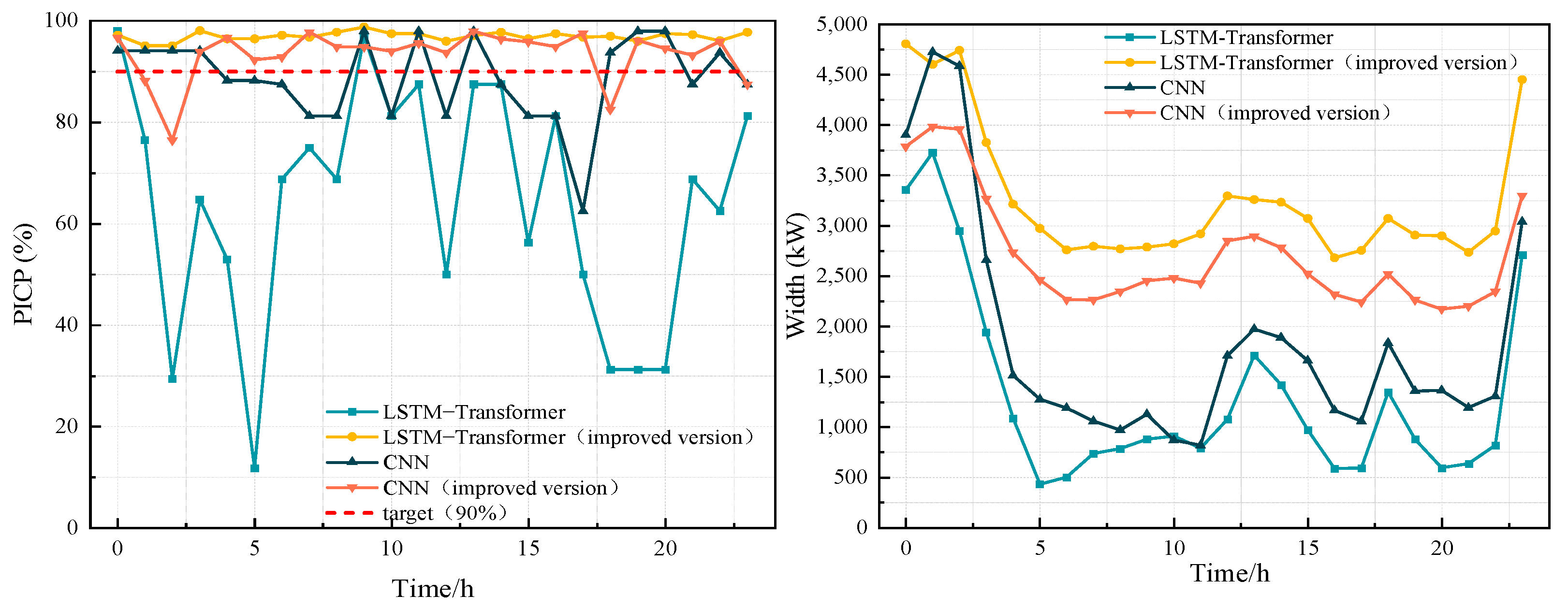
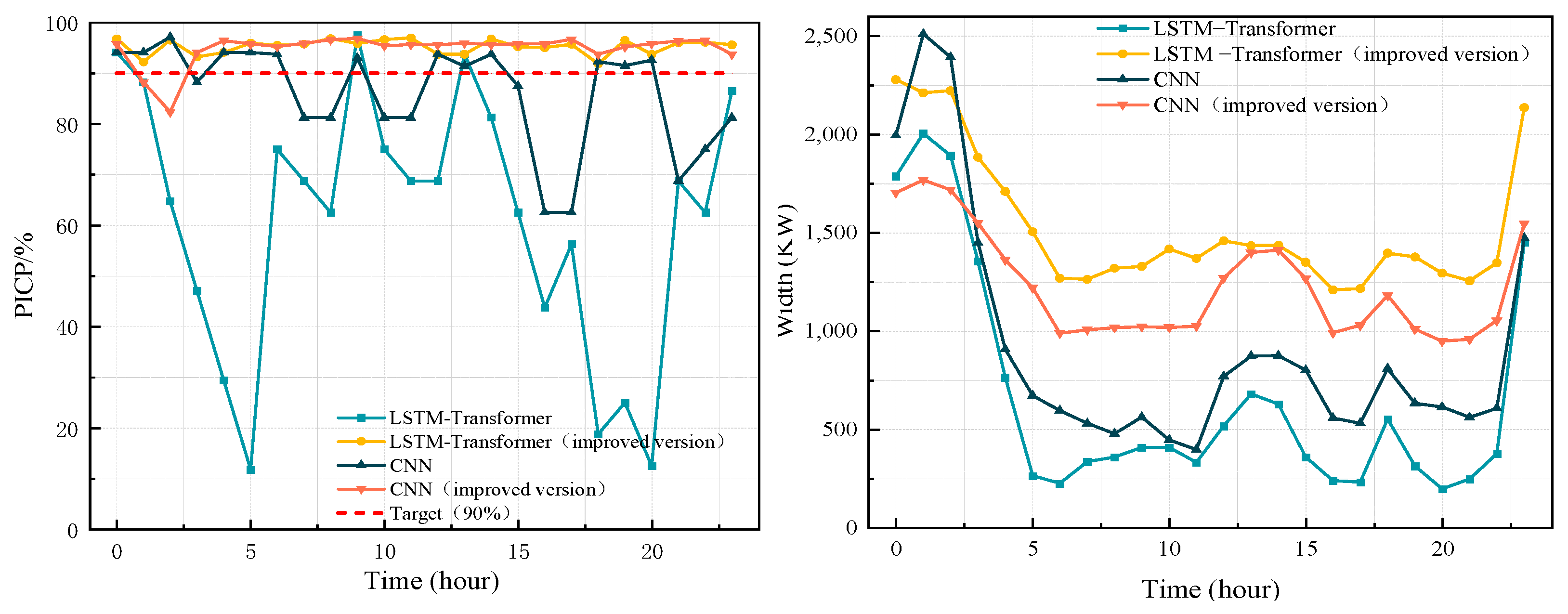
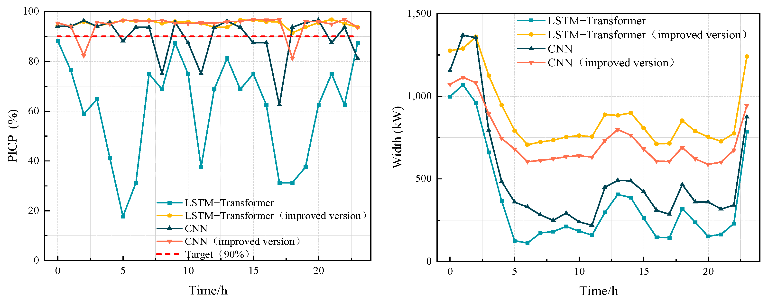
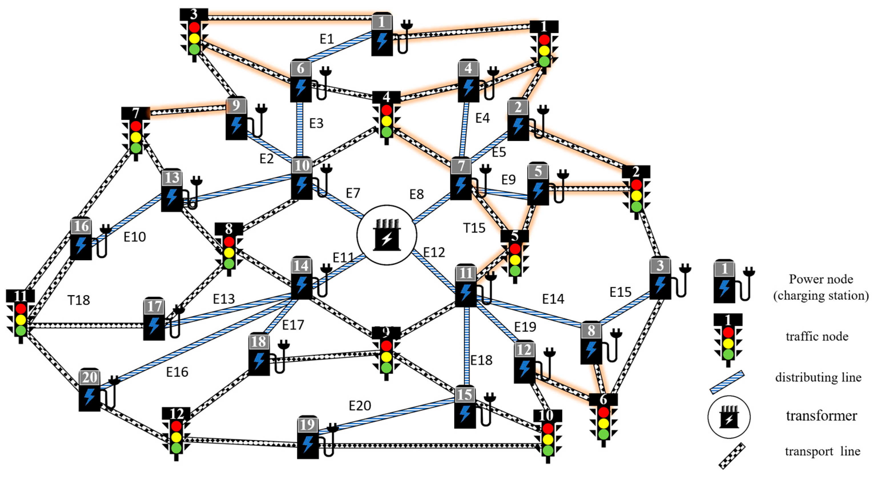
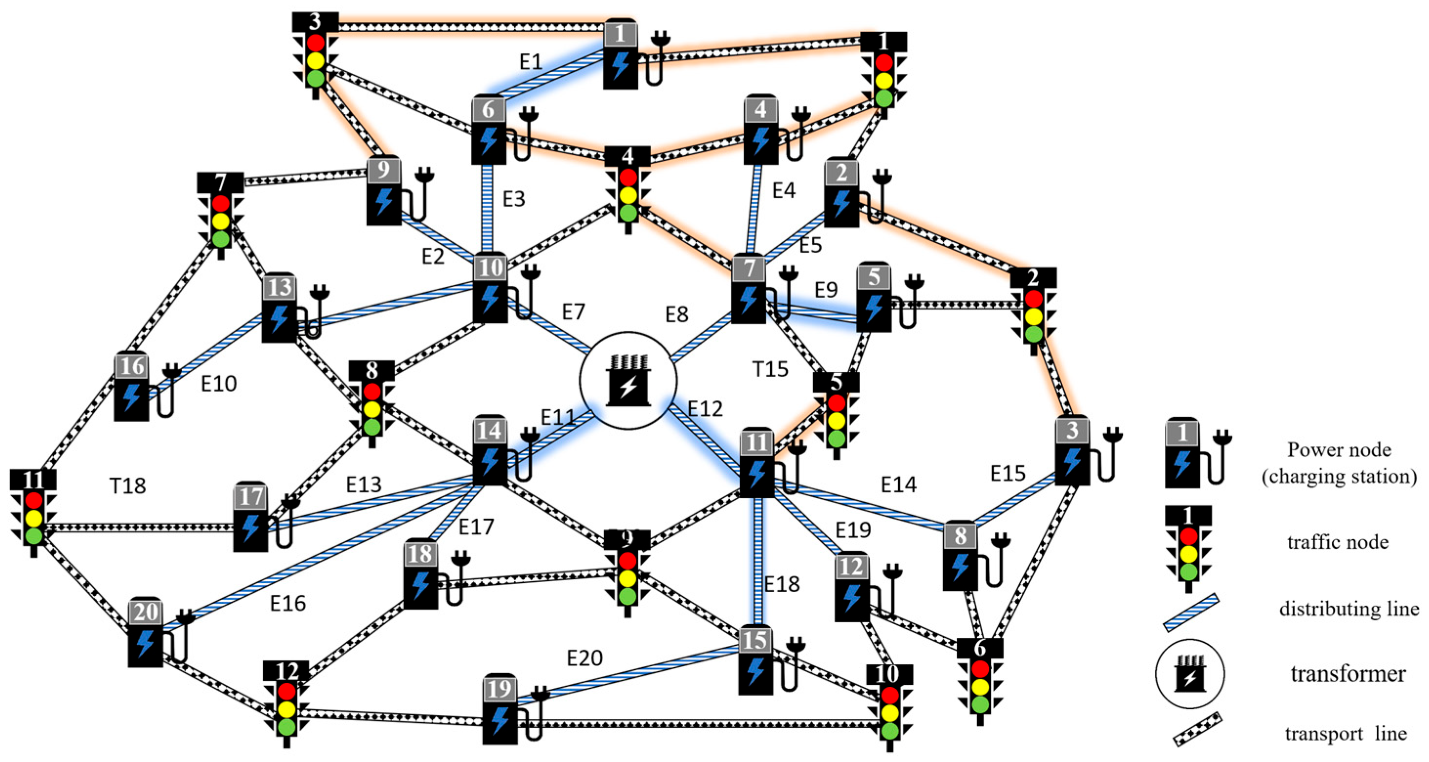
This study develops a coordinated modeling framework integrating data-driven methods with physical mechanisms. It enhances the resilience of urban power–transportation systems under extreme disturbances. A fully automatic density-based clustering method addresses cross-infrastructure data heterogeneity. Nodal loads, line-loading rates, and road traffic flows are dynamically segmented. Trend and statistical features are then extracted from each segment. A reference time-series is selected for centroid matching across the three data types. This process aligns the heterogeneous timeseries into corresponding scenario classes.
Building on this framework, an LSTM–Transformer model with quantile regression is developed. The LSTM–Transformer extracts temporal features from power loads and traffic flows. Quantile regression estimates conditional quantiles and constructs prediction intervals. Together, these components enable accurate interval forecasts of future loads and traffic flows. Meanwhile, a coupled indicator system characterizes operational risk. It includes nodal load ratios, distribution-line loading ratios, and traffic delays. The three-sigma rule classifies these indicators into multiple risk levels. A multilevel penalty mechanism then balances economic efficiency and operational security. Finally, a capacity planning model is established for resilience enhancement. The model follows a three-stage logic of investment, evaluation, and optimization. Coordinated decisions are then made to reinforce key power lines, expand traffic corridors, and increase charging-node capacity. These decisions enhance the robustness of the power–transportation-coupled network under extreme scenarios. They also support optimal resource allocation.
2.1. Feature Identification and Differentiated Scenario Classification of Power Load and Traffic Flow Based on Fully Automatic Density-Based Clustering
2.1.1. Hierarchical Processing of Temporal Features
The study objects include two types of infrastructure elements: nodes and links. The operation or usage behavior of different objects can be uniformly characterized by time-series. For load nodes, the behavior is represented by nodal load-power time-series. For distribution lines, the behavior is represented by line-loading-rate time-series. For road links, the behavior is represented by traffic-flow time-series.
Therefore, the original behavior of any node or link can be abstracted as a one-dimensional time-series: .
To eliminate scale differences and mitigate noise effects, min–max normalization is first applied to the time-series, as shown in Equation (1):
In Equation (1), xv denotes the original data. xmax and xmin denote the maximum and minimum values within the statistical period, respectively. denotes the normalized sequence.
Furthermore, sliding-window averaging is used to smooth the normalized sequence. This step mitigates the effect of short-term random disturbances on feature extraction. Let
w denote the half-window length. The calculation is shown in Equation (2).
In Equation (2), = 2. Node and link behaviors are usually nonstationary. Direct analysis of the complete time-series may obscure local behavioral features. Therefore, a time-series segmentation method based on a dynamically growing window is adopted.
A time-series with length III is dynamically segmented. The time-series is divided into mf segments. Accordingly, mf − 1 segmentation points are identified . Time-series data are then introduced point by point into the dynamically growing window. The fitting error SSEq is calculated in real-time. The threshold SEPmax is set according to the overall noise level of the original sequence. When the error within the window exceeds the preset threshold SEPmax, the current time point is identified as the segmentation point tv. The current segment is then terminated, and a new segment is initialized. The initial segment is set to start from the beginning of the sequence. When the segmentation point is detected, the first n data points are assigned to the first segment. The range of the current segment is defined using the segmentation-point set . Thus, segment q is expressed in .
For each time-series segment, low-dimensional features are extracted from two aspects. These aspects include trend characteristics and statistical characteristics. Trend characteristics are obtained by fitting each segment with a low-order polynomial. The fitting coefficients reflect the overall trend of the segment. Statistical characteristics are represented by variance, skewness, and the autocorrelation coefficient. Their calculation formulas are shown in Equations (3)–(5).
The above features are combined to obtain the low-dimensional feature vector of each segment, as shown in Equation (6).
In Equation (6), pq denotes the polynomial approximation parameters of segment q.
To unify the feature dimensions of different nodes and links, hierarchical clustering is performed on all segment features. These features are then divided into a fixed number of behavioral categories. For each segment category, the cluster centroid and extreme segments are extracted. Here, denotes the time-series index, and T denotes the number of time-series. denotes the cluster index in each time-series, and k denotes the number of clusters. Subsequently, one time-series is selected as the reference. Its segment clustering results are matched with the cluster centroids of other time-series. Cross-object category alignment is then completed. Each original timeseries is further mapped into a sequence composed of category labels . The above method provides fundamental inputs for subsequent differentiated scenario analysis and the coordinated decision-making model of nodes and links.
2.1.2. Fully Automatic Density-Based Clustering Algorithm
Through hierarchical temporal-feature processing, high-dimensional nonstationary time-series are transformed. These series are from the original nodes and links. They are converted into structurally unified low-dimensional feature representations. Based on local density distributions in the feature space, a fully automatic adaptive density-based clustering method is introduced. This method robustly identifies behavioral categories of nodes and links. Specifically, it identifies residential, commercial, and industrial patterns under holiday and non-holiday scenarios.
After hierarchical temporal-feature processing and mapping, node and link samples are represented as a point set. This point set is embedded in the feature space, as shown in Equation (7).
In Equation (7), denotes the low-dimensional feature vector of the i-th node or link sample.
In density-based clustering, the neighborhood radius Eps is a key parameter for characterizing the local density structure. Its value directly affects the stability and rationality of the clustering results. To avoid the subjectivity caused by manual parameter setting, the neighborhood radius is determined adaptively. This determination is based on the distribution characteristics of nearest-neighbor distances among sample points in the feature space.
For any feature point
Pvi, the Euclidean distance between
Pvi and its nearest-neighbor sample point
Pvj is calculated, as shown in Equation (8).
The above calculation is repeated for all sample points. The nearest-neighbor distance set is then obtained, as shown in Equation (9).
To eliminate scale differences among different datasets, the distance set D is normalized. Its distribution is then statistically analyzed. A nearest-neighbor distance histogram is constructed. This histogram characterizes the overall density structure of samples in the feature space.
Let
μd and
σd denote the mean and standard deviation of the nearest-neighbor distance set, respectively. Their calculation is shown in Equation (10).
To characterize the density dispersion of samples in the feature space, the adjustment coefficient λ
b is defined as the coefficient of variation in the nearest-neighbor distance distribution, as shown in Equation (11).
In Equation (11), ε is a very small positive constant. It is introduced to avoid division by zero.
Let
dmax and
dmin denote the maximum and minimum nearest-neighbor distances of sample points, respectively. The distance distribution range and the density dispersion of samples are jointly considered. The final neighborhood radius Eps expressed in Equation (12).
In Equation (12), λ is used to balance clustering compactness and noise tolerance.
After the neighborhood radius Eps is determined, another key parameter in density-based clustering is the minimum number of neighboring points,
MinPts. This parameter is used to determine whether a sample point is a core point in a high-density region. For any sample point Pi, the number of neighboring points within the radius Eps is counted, as shown in Equation (13).
The number of neighboring points is calculated for all sample points. The neighboring-point-count set is then obtained, as shown in Equation (14).
The distribution characteristics of this set are statistically analyzed. A clear central tendency is observed in most datasets. Therefore, the high-frequency values in the neighboring-point-count distribution are selected as candidate values of MinPts. These values reflect the most representative local density level in the dataset.
The adaptive neighborhood radius Eps is first obtained. The minimum neighborhood point count MinPts is also determined. Density-based clustering is then performed on sample points embedded in the feature space. This process identifies high-density regions. It groups nodes or links with similar behavioral characteristics. For any data point Pv, a neighborhood centered at Pv is constructed with radius Eps. The number of points ni within this neighborhood is then calculated. When , point Pi is identified as a clustering core point. If no labeled samples exist in the neighborhood of a core point, a new cluster label is assigned. If a labeled core point already exists, the point is merged into the corresponding cluster. This operation ensures label consistency within local high-density regions. When , point Pi is regarded as a non-core point. If a labeled core point exists within its neighborhood, the sample point is assigned to the cluster of the nearest core point. Otherwise, the sample point is retained as a potential outlier.
Through the automatic adaptive density-based clustering process, node and line samples are mapped to behavior-category labels in the embedded feature space. Let
denote the clustering label mapping function. Each sample
Pi is assigned to the corresponding behavior class
Ck or the outlier set O, as shown in Equations (15) and (16).
In Equations (15) and (16), denotes that sample Pi belongs to the r-th regional category. This category includes industrial, commercial, and residential areas. It also belongs to the s-th scenario category. The scenario category is either holiday or non-holiday. denotes that sample Pi is identified as an outlier.
2.2. Hybrid Deep Learning-Based Interval Forecasting Method for Coupled Load and Traffic Flow
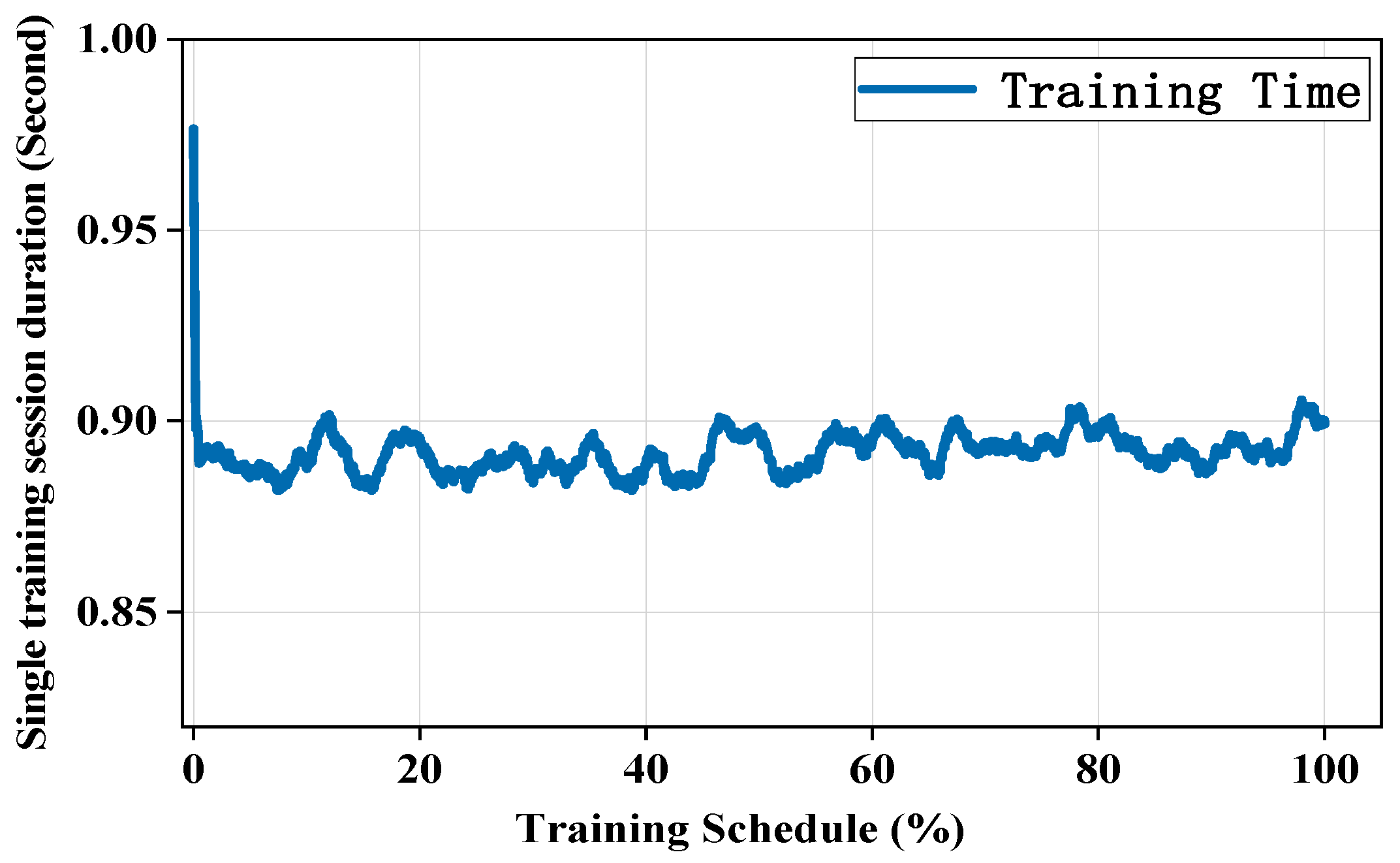
To achieve high-accuracy interval forecasting under the two scenario types, a hybrid deep learning framework is developed. The target variables include load variations at power nodes and power lines. They also include traffic-flow variations in traffic links. The framework integrates LSTM and Transformer modules in a unified architecture. On this basis, a quantile regression mechanism is incorporated. The model outputs statistically meaningful prediction intervals. These intervals quantify forecasting risks caused by traffic behavior, load characteristics, and other uncertainties. The data organization mechanism is first described. The LSTM–Transformer serial backbone is then introduced. The interval output layer is subsequently presented. Finally, the overall training and prediction procedure is explained.
First, a scenario-driven data organization mechanism is constructed. The historical observation dataset is defined in Equation (17):
where power nodes, power lines, and transportation links
rt denote the regional label. The labels correspond to industrial, commercial, and residential areas, respectively.
In Equation (17), t denotes the time index. T denotes the time horizon. xt denotes the raw input feature vector at time t. It has dimension d. The samples are divided into three entity types. These types are power nodes, power lines, and traffic links. The clustering process assigns scenario label s and regional label r. The model then outputs yt. yt denotes the target variables. These variables include electrical load and traffic flow. denotes the scenario label. It is determined by the previous automatic density-based clustering of electricity-consumption features. denotes the holiday scenario, whereas denotes the non-holiday scenario. et denotes the entity-type label. It includes power nodes, power lines, and traffic links rt denotes the regional label. The labels correspond to industrial, commercial, and residential areas, respectively.
For any given scenario–type–region combination (
s,
e,
r), the corresponding dedicated training subset is defined in Equation (18).
Based on this subset, a sliding-window input sequence with length H is constructed.
In Equation (19), HHH denotes the length of the historical time window.
The objective is to forecast the one-hour-ahead prediction interval, as shown in Equation (20)
In Equation (20), and denote the lower and upper prediction bounds, respectively.
The LSTM network selectively memorizes and forgets long-sequence information through gating mechanisms. It is suitable for capturing short-term fluctuations and temporal accumulation effects in load and traffic flow sequences. Its information-processing procedure consists of four key steps:
In Equation (21), ft denotes the forget gate. represents the sigmoid activation function. Wf, ht−1, xt, and bf denote the weight of the forget gate, the hidden state at time t − 1, the input at time t, and the bias of the forget gate, respectively.
The second step is input gate calculation. It filters the new information from the current input that needs to be written into the memory cell, as shown in Equations (22) and (23)
In Equations (22) and (23), it denotes the input gate. denotes the candidate memory cell state. Wi and Wc represent the weights of the input gate and candidate memory cell state, respectively. bi and bc represent their corresponding biases.
The third step is memory cell update. It integrates the historical information selected by the forget gate and the new information selected by the input gate. The memory cell at the current time step is updated, as shown in Equation (24).
In Equation (24), Ct−1 and Ct denote the memory cell states at time t − 1 and time t, respectively.
The fourth step is output gate calculation. It generates output information based on the updated memory cell. It also determines the current hidden state, as shown in Equations (25) and (26).
In Equations (25) and (26), Ot denotes the output gate. Wo and bo represent the weight and bias of the output gate, respectively. ht denotes the hidden state at the current time step.
After LSTM processing, the original measurement sequence is mapped into a high-dimensional feature representation with rich temporal semantics. This representation serves as the input to the subsequent Transformer module. The core procedure is described as follows:
First, positional encoding is introduced into the hidden-state sequence output by the LSTM. This operation preserves temporal information. Then, the encoded sequence passes through stacked Transformer encoder layers. Each encoder layer consists of multi-head self-attention and a feed-forward neural network. Residual connections and normalization improve training stability and convergence speed. The multi-head self-attention mechanism computes interactions among queries, keys, and values in parallel. These interactions are computed across multiple subspaces. The mechanism dynamically assigns attention weights among different time steps. Finally, the last time step of the final Transformer encoder output is selected as the context representation. This representation is fed into the interval prediction output layer for quantile regression. It enables accurate one-hour-ahead interval estimation of load and traffic-flow variations. The estimation is performed for power nodes, power lines, and traffic links under holiday and non-holiday scenarios.
The computational form of the multi-head self-attention mechanism is shown in Equations (27)–(29).
In Equations (27)–(29), Q, K, and V denote the query, key, and value matrices, respectively. Wo denotes the learnable output projection matrix. , , and represent the projection matrices of the query, key, and value matrices, respectively. Dk denotes the dimension of the key.
Quantile regression is used to output the prediction interval. Two linear output heads are defined, as shown in Equations (30) and (31).
In Equations (30) and (31), denotes the feature vector output by the LSTM–Transformer hybrid model at time t. Wα and W1−α denote the learnable weight vectors for predicting the lower and upper quantiles, respectively. bα and b1−α denote the learnable bias terms for predicting the lower and upper quantiles, respectively. α is the predefined quantile level. It controls the confidence level of the prediction interval.
2.3. Evaluation Metrics for Deep Learning-Based Prediction
The probabilistic forecasting results in this simulation are comprehensively evaluated using three types of metrics: reliability, sharpness, and the Pinball score [
27].
- (1)
Reliability Metric
The prediction interval coverage probability, abbreviated as PICP, is used to evaluate interval reliability. It measures whether the prediction interval properly contains the actual observations. A coverage probability closer to the confidence level α indicates higher forecasting reliability. For any probabilistic forecasting result, the PICP is calculated as shown in Equations (32) and (33).
In Equations (32) and (33),
EDev, α denotes the deviation index. It is used to evaluate the unbiasedness of probabilistic forecasting results. U denotes the total number of samples.
denotes the indicator function of the v-th sample. Its definition is given in Equation (34).
In Equation (34), and denote the predicted upper and lower bounds of the v-th sample at the confidence level α, respectively.
- (2)
Sharpness Metric
The sharpness metric reflects the width or dispersion of the prediction interval. It is used to evaluate the precision of probabilistic forecasting information. In this study, sharpness is measured using the standardized root-mean-square width of the prediction interval. This metric reflects the dispersion degree of the probabilistic forecasting distribution. A smaller sharpness value indicates a more concentrated prediction distribution and better forecasting performance. The sharpness at confidence level α\alpha α is calculated as shown in Equation (35).
In Equation (35), R denotes the difference between the predicted maximum and minimum values of the v sample.
- (3)
Pinball Score Metric
The Pinball score is a standard loss function for quantile regression. It captures both the direction and magnitude of prediction errors. It also reflects the reliability and sharpness of forecasting results. A smaller Pinball score indicates better probabilistic forecasting performance. The Pinball score is calculated as shown in Equations (36) and (37).
In Equations (36) and (37), X pinball denotes the average Pinball score of the probabilistic forecasting results. denotes the Pinball score of the v sample at quantile level d represents the index of the quantile level.
2.4. Computational Method and Resilience Evaluation Metrics for the Coupled Power–Transportation Network
2.4.1. Calculation of the Coupling Relationship Between Power Load and Traffic
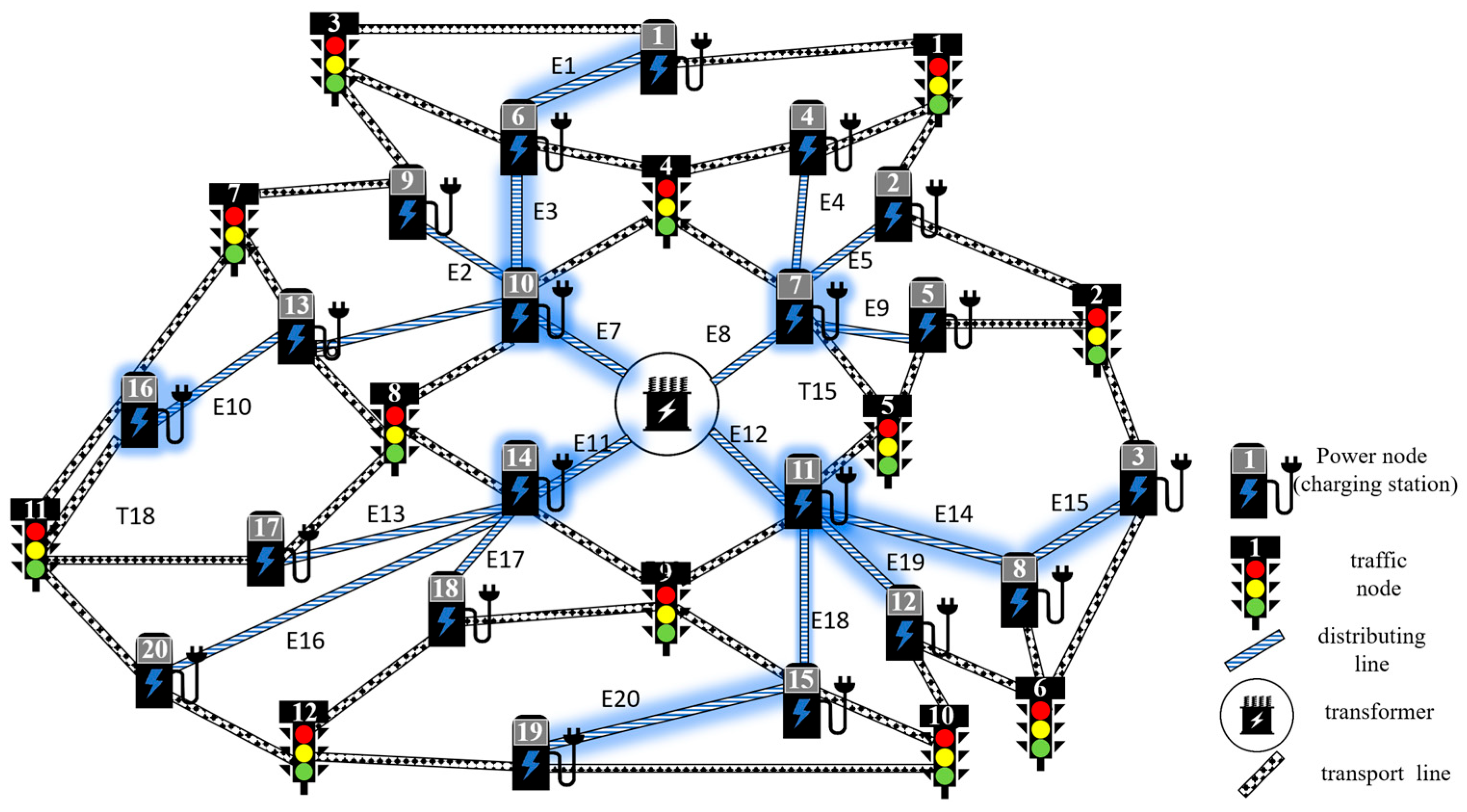
Flow in this study, power–transportation coupling is represented at grid nodes. The base load of each node is added to the electric vehicle charging load. The total load of each node in different functional regions is then obtained. Its mathematical expression is given in Equation (38).
In Equation (38),
denotes the total load of node
i in region a.
denotes the base load of node
i in region a. N denotes the number of electric vehicles charging at distribution network node
i around time t.
denotes the charging power of electric vehicle
j at distribution network node
i at time t [
28].
In practice, EV drivers exhibit bounded rationality. Their decisions are influenced by personal preferences and navigation systems. Therefore, they may not strictly follow dispatch instructions. A discrete logit choice model is therefore established. It estimates the probability of selecting each feasible route. These routes connect the same origin and destination but have different lengths [
29].
In Equation (39), ϕm denotes the probability that a driver selects route m. cm and cn denote the generalized travel costs of routes m and n, respectively. K denotes driver sensitivity to travel-time costs. M denotes the set of all available routes. Ξ denotes the detour threshold, and β denotes the detour penalty coefficient.
2.4.2. Calculation Method for Resilience Evaluation Metrics of the Coupled Network
In capacity-configuration modeling for the coupled power–transportation system, a differentiated penalty mechanism requires prior uncertainty quantification. The considered key performance indicators include the power-node load carrying ratio, power-line transmission carrying ratio, and traffic delay time. Their risk levels are then classified. Based on the joint prediction intervals of load and traffic flow obtained by the LSTM–Transformer hybrid model, the prediction intervals of these three indicators are further derived. Their risk levels are classified according to the three-sigma principle. This classification provides a mathematical basis for introducing interval-dependent penalty terms into the subsequent cost function.
- (1)
Calculation of the Power-Node Load Carrying Ratio
To evaluate the supply margin and overload risk of power nodes under specific operating states, the load carrying ratio is adopted as the assessment metric. This metric reflects the proportion of the current load demand to the available supply capacity of a node. Its specific expression is shown in Equation (40).
In Equation (40),
denotes the maximum local generation capacity of node i.
Based on the above load prediction interval, the calculation interval of this metric is obtained as shown in Equation (41).
In Equation (41), and denote the upper and lower bounds of the node load carrying ratio, respectively. and denote the upper and lower bounds of the load of node iii at time t, respectively. The interval forms of the power-line transmission carrying ratio and traffic delay time are derived in the same manner.
- (2)
Calculation of the Power-Line Transmission Carrying Ratio
The power-line transmission carrying ratio represents the ratio of the current transmitted power to the thermal stability limit of a line. It is an important metric for evaluating the operating state of the line. Its specific calculation form is shown in Equation (42).
The calculation interval of the power-line transmission loading rate is denoted by .
In Equation (42), fl,t denotes the actual active power flow of line l at time t. denotes its maximum allowable transmission capacity. xl,t denotes the reactance of line l at time t. and denote the voltage phase angles of nodes u and v, respectively.
- (3)
Traffic Delay Time
Under ideal assumptions, the number of vehicles that a single lane can accommodate equals the road length divided by the sum of the average vehicle length and the front and rear safety distances. If there are r types of roads, the carrying capacity C of the entire transportation network is the sum of the carrying capacities of all roads. The saturation intervals of different road sections are then obtained, as shown in Equation (43).
The prediction interval of traffic flow is denoted by
. The corresponding saturation interval is then calculated as
. By further considering the dynamic traffic flow on the road, the travel-time equation for passing through this road section is obtained, as shown in Equation (44).
t0 denotes the free-flow travel time through this road section. It is calculated as shown in Equation (45).
The delay time is then denoted by . Its prediction interval is expressed as .
In Equation (43), Cj denotes the theoretical carrying-capacity set of the j-th road section. W and denote the road width and lane width, respectively. L denotes the road length. l and s denote the average vehicle length and the safety distance between vehicles, respectively. denotes the saturation of the j-th road section at time t. qj,t denotes the traffic flow of the j-th road section at time t.
Although the above intervals reflect uncertainty, the continuous intervals need to be divided into several discrete risk levels. This division facilitates the introduction of a piecewise penalty mechanism into the cost function. In this study, the indicators are standardized and then classified according to the 3σ principle.
The actual values of each indicator are assumed to follow an approximately normal distribution centered on the predicted median. Let
denote a given indicator, and let
denote its prediction interval. The predicted median and half-width are expressed in Equations (46) and (47)
In Equations (46) and (47), denotes the predicted median, and denotes the predicted half-width.
Based on
and
, the indicator space is divided into three risk-level intervals. The first interval is the low-risk region R1. In this region, the operating state is normal, and no additional penalty is imposed. The second interval is the medium-risk region R2. In this region, the operating state approaches its boundary, and a moderate penalty is imposed. The third interval is the high-risk region R3. In this region, limit violations are highly likely, and a high penalty is imposed. The specific classification of the three regions is shown in Equations (48)–(50).
Based on the above classification, the risk level
of any indicator
Xt can be determined using an indicator function, as shown in Equation (51).
When the risk level is 1, no penalty is imposed. When the risk level is 2, the penalty cost is μ1. When the risk level is 3, the penalty cost is μ2.
2.5. Capacity Planning Model Considering Coupled-Network Resilience
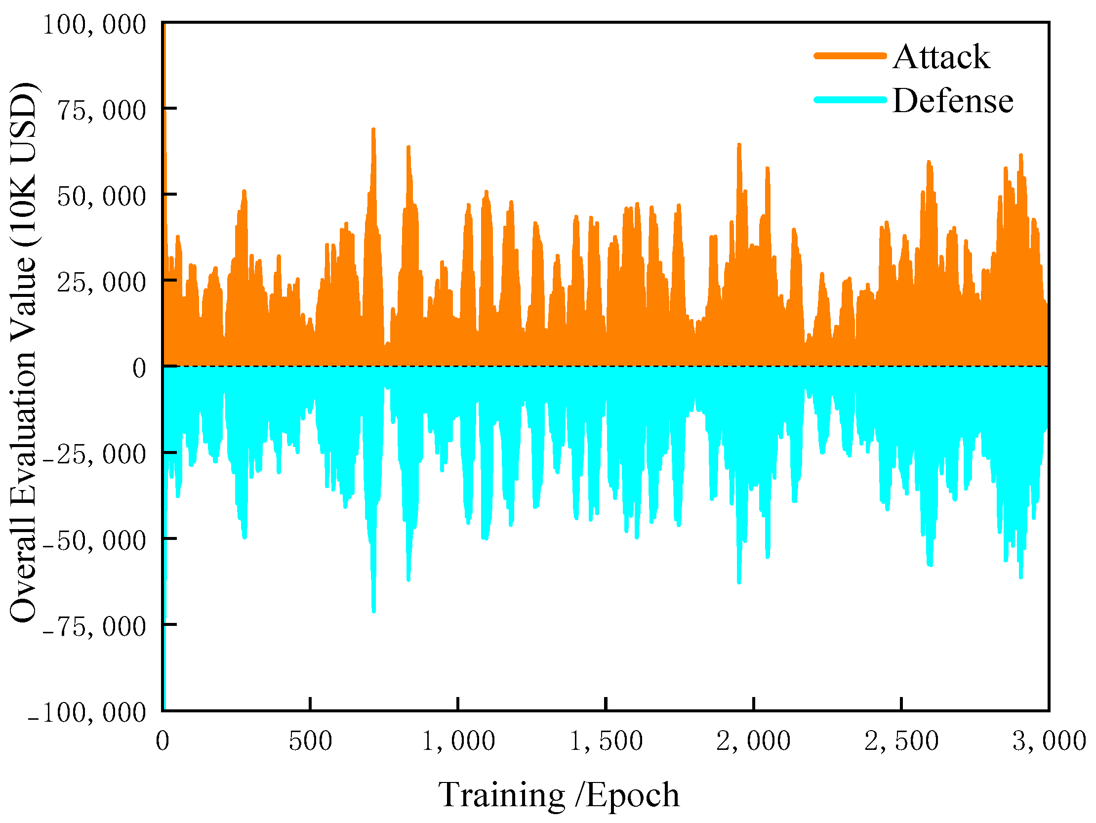
To characterize the capacity planning problem of the coupled power–transportation network under urban resilience constraints, a tri-level resilience enhancement model is constructed. The upper level determines the investment planning scheme. Its objective is to minimize the sum of investment cost and operating cost under the worst-case scenario. The middle level searches for the disturbance scenario that maximizes the system operating cost. This search is based on the scheme given by the upper level. The lower level performs dispatch under the worst disturbance scenario identified by the middle level. It then calculates the minimum operating cost of the system.
For mathematical modeling, the distribution network and transportation network are both represented as directed graphs. NP and LP are defined as the sets of all nodes and branches in the distribution network, respectively. In the radial distribution network , the node set consists of the slack bus and the remaining buses. In the connected transportation network graph , NT and LT denote the sets of all nodes and links in the transportation network, respectively.
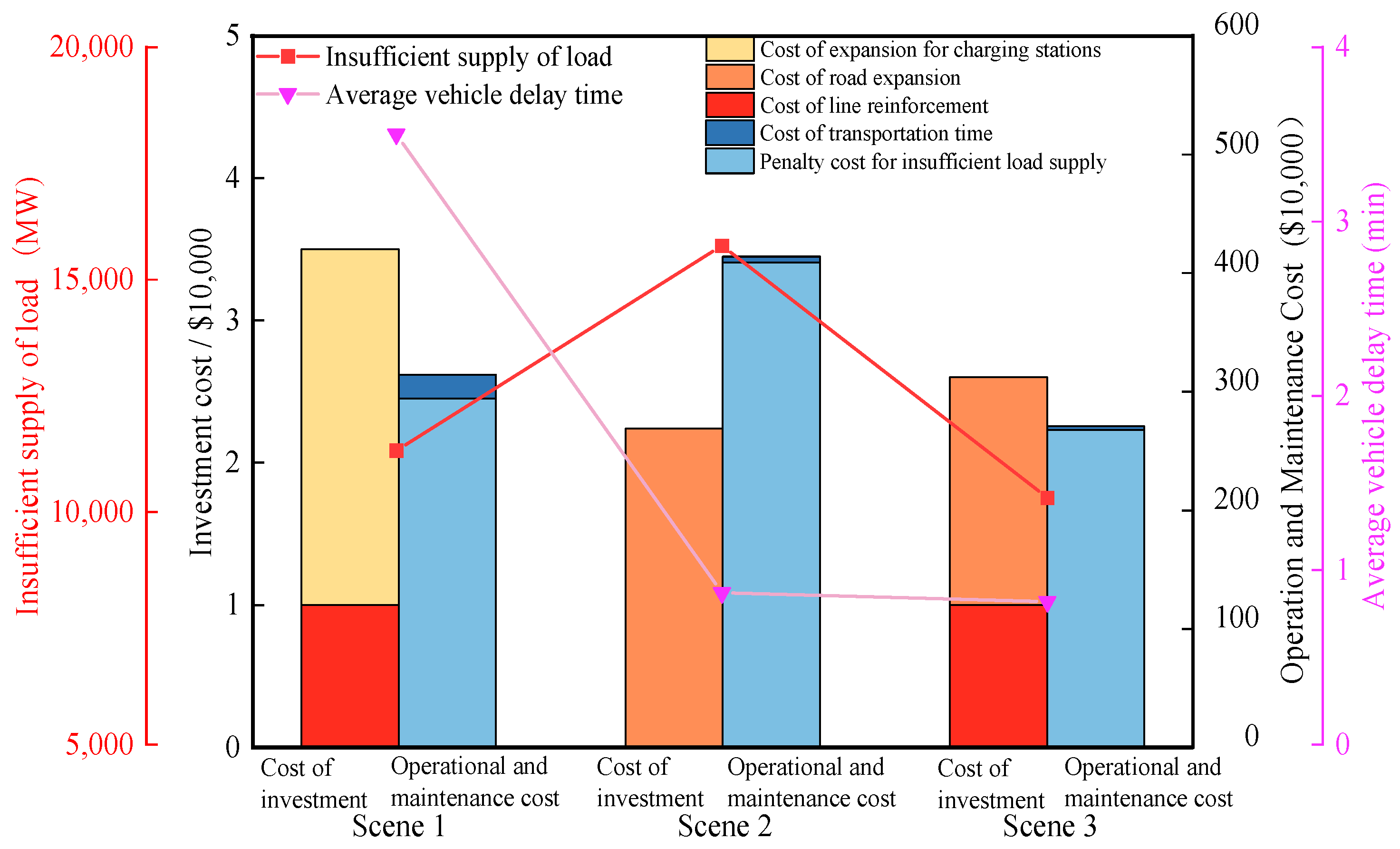
The upper level of the model corresponds to the first stage. It determines the long-term infrastructure layout before abnormal events occur. In this stage, upfront investment is used to enhance the ability of the coupled network to withstand extreme disturbances. Critical lines and nodes that are vulnerable to load shocks in the power network are identified. This identification determines whether line reinforcement and node capacity expansion should be implemented. Meanwhile, bottleneck road sections that are prone to congestion in the transportation network are evaluated. This evaluation determines whether road expansion should be implemented.
The decision variables include whether power lines should be reinforced, whether transportation roads should be expanded, and whether charging piles at power nodes should be expanded. The objective function is shown in Equation (52).
In Equation (52),
and
denote the pre-event investment costs for infrastructure construction in the distribution network and transportation network at node iii, respectively, as shown in Equation (53).
In Equation (53), μl denotes the reinforcement cost of power line l. yl is a binary variable indicating whether power line l is reinforced. μl denotes the unit expansion cost of charging piles at power node i. Ni denotes the set of binary variables indicating whether charging piles at power node I are expanded. μj denotes the expansion cost of road section j ωj is a binary variable indicating whether road section j is expanded.
The second stage is based on the optimal investment scheme determined by the upper level. It dynamically adjusts power load and traffic flow distributions by determining the disturbance coefficients of power lines and transportation links. This stage simulates the impact of extreme disturbances on the coupled network. Within the allowable fluctuation range, it searches for the disturbance combination that maximizes the system operating cost. This process identifies defense blind spots that are not covered by the investment scheme. The objective function of this stage is shown in Equation (54).
In this equation, and denote the operating costs of the power grid and transportation network, respectively. ul and uj denote the state variables of power line l and traffic road section j, respectively. A value of 0 indicates no overload, whereas a value of 1 indicates overload. denotes the budget set of the attacker’s disturbance vector.
The third stage aims to simulate the system operating state under the combined effects of investment decisions and extreme disturbances. Based on the investment scheme determined in the first stage, the minimum system operating cost is calculated under the disturbance scenario specified in the second stage.
To facilitate the subsequent analysis, the loading-rate limits of power nodes and power lines are set as
ps and
λs, respectively. The delay-time limit of traffic links is set as
ts. In this stage, the objective function for minimizing the total operating cost is formulated in Equations (55) and (56).
In Equations (55) and (56), denotes the purchased power at power node i. ai denotes the average power purchase cost per unit power at power node I, denotes the load-shedding power at power node i. bi denotes the average load-shedding penalty cost per unit power at power node i. al and bl denote the average power transmission operation and maintenance cost per unit power and the penalty cost per unit power exceeding the transmission limit of power line l, respectively. denotes the transmitted power of power line l. denotes the curtailed power of power line l. μt denotes the time-to-cost conversion coefficient of the transportation network. tj denotes the travel time of traffic link j. qj denotes the traffic flow of traffic link j.
The distribution networks connected to EV charging stations are considered radial networks. To prevent overload on power line
i, the line power transmission limit is imposed, as shown in Equation (57).
In Equation (57), and denote the lower and upper transmission limits of power node iii, respectively. and denote the lower and upper transmission limits of power line i, respectively.