Decision-Focused Wind Power Forecasting for Economic Dispatch Under Asymmetric Imbalance Costs

Abstract

Wind power forecasts are commonly trained to minimize statistical errors, although the thermal schedule based on a forecast ultimately incurs asymmetric recourse costs. To connect forecast training with this dispatch consequence, a dispatch-value-oriented forecasting (DVOF) framework is developed by coupling a Mamba-style forecaster with a solver-based differentiable economic-dispatch layer. The forecast determines the first-stage thermal schedule; after wind realization, load shedding and wind curtailment settle the imbalance, and the resulting recourse-cost gradient is propagated to the forecaster by KKT-based implicit differentiation. On Global Energy Forecasting Competition 2014 (GEFCom2014) data, DVOF reduces the day-ahead realized imbalance penalty from $55.5$ to $26.6$ cost units per hour relative to an MSE Loss model with the same backbone. The resulting forecast approaches the conservative operating point implied by the asymmetric recourse model. In the simplified single-area, single-period case, this result shows that the dispatch gradient can guide the forecaster toward a cost-relevant adjustment without prescribing or searching over a quantile level.

1. Introduction

With the transition toward low-carbon power systems, wind power has become an increasingly important source of electricity supply. According to the Global Wind Report 2026, global cumulative installed wind power capacity reached 1299 GW in 2025 and is expected to continue increasing in the coming years [1]. Despite its environmental benefits, wind generation remains inherently weather-dependent and nondispatchable. Its variability and uncertainty affect generation scheduling, economic dispatch, reserve scheduling, and balancing operations [2,3]. Therefore, reliable wind power forecasts (WPFs) are essential inputs to the secure and economic operation of wind-rich power systems [4,5].

Over the past decades, a large number of studies have been devoted to improving wind power forecasting models. Early approaches mainly relied on physical models and numerical weather prediction (NWP). In these methods, meteorological variables are converted into wind power estimates using hub-height wind estimation, turbine power curves, and site-specific corrections. Although physical methods are interpretable, their performance can be affected by NWP errors, terrain complexity, and model mismatch. To reduce reliance on detailed physical modeling, statistical methods [6] were introduced to capture temporal dependence directly from historical wind power data. With the increasing availability of supervisory control and data acquisition (SCADA) data, machine learning methods further improved forecasting performance by learning nonlinear relationships between meteorological inputs and power outputs [7]. More recently, deep learning models, such as recurrent neural networks (RNNs) [8,9], convolutional neural networks (CNNs) [10,11], and attention-based models [12,13,14], have been widely used to model temporal and multi-scale wind patterns. These methods have substantially improved forecast accuracy and provided system operators with more reliable inputs for generation scheduling and economic dispatch.

Despite these advances, wind power forecasting remains challenging because wind power exhibits rapid local fluctuations as well as long-range dependencies driven by meteorological evolution. Extending the input context can provide richer temporal information but also increases the computational burden, particularly for self-attention-based models whose complexity grows quadratically with sequence length. Selective state-space models, exemplified by Mamba, provide an efficient alternative by introducing input-dependent state transitions and processing a length-T sequence in $O\left(T\right)$ time [15,16]. Existing Mamba-based WPF studies have focused primarily on improving statistical forecast accuracy, whereas their integration with downstream economic dispatch for decision-focused or value-oriented training remains insufficiently explored.

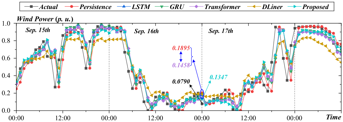
In power system operation, a WPF is not merely a standalone statistical output. It serves as an input to generation scheduling before wind power is realized. In a two-stage forecast-based economic dispatch process, the WPF affects the first-stage generation schedule, whereas the deviation revealed upon wind power realization gives rise to the subsequent balancing requirement [17]. Therefore, two forecasts with the same mean absolute error (MAE) or mean squared error (MSE) can induce different realized recourse costs. For example, suppose that the realized wind power is $0.50$ p.u. Forecasts of $0.45$ and $0.55$ p.u. have the same absolute error and are therefore equivalent under MAE. However, from an operational perspective, they may lead to different consequences. A forecast of $0.55$ p.u., which overestimates the realized wind power, may result in insufficient scheduled thermal generation, thereby increasing the need for upward balancing and, in extreme cases, load shedding. In contrast, a forecast of $0.45$ p.u., which underestimates the realized wind power, increases scheduled thermal generation and may therefore reduce shortage risk at the expense of greater wind curtailment when the realized wind power is high. When overforecasting and underforecasting have asymmetric operational consequences, symmetric statistical losses cannot distinguish between equal-magnitude errors of opposite signs [18]. Therefore, a forecast should be evaluated not only by its statistical accuracy but also by the realized second-stage recourse cost induced by its forecast-based generation schedule. However, most existing wind power forecasting approaches, including advanced deep learning models, are still trained using conventional statistical losses and evaluated primarily using forecast-accuracy metrics [19]. They do not explicitly account for the impact of forecast errors on first-stage dispatch decisions and second-stage recourse costs [20,21]. Therefore, it is necessary to study whether higher forecast accuracy necessarily leads to lower realized recourse cost.

The literature bearing on this accuracy–value mismatch falls into four streams, which the following two paragraphs address in turn. These are cost-oriented and probabilistic renewable forecasting, decision-focused learning and differentiable optimization, forecasting–optimization integration for trading and commitment, and forecasting under imbalance settlement in power-system operation.

The first stream designs forecast products according to downstream operational consequences. For example, Ref. [20] proposed cost-oriented prediction intervals and showed that statistically calibrated intervals do not necessarily minimize downstream operating cost. Moreover, Ref. [21] considered contextual selection of value-oriented prediction intervals, allowing the preferred interval to change with the operating condition. Both build on the asymmetric quantile-regression loss introduced by [22], whose minimizer is the conditional quantile of the target. These approaches exploit the asymmetry between power shortfalls and surpluses by selecting decision-relevant forecast products without explicitly differentiating through the downstream optimization problem. The second stream uses end-to-end decision-focused learning together with differentiable optimization. Ref. [23] proposed the Smart "Predict, then Optimize" framework, in which predictions are evaluated according to the decision loss they induce rather than solely by their deviation from the realized outcome. Earlier, Ref. [24] trained a probabilistic model directly against the cost of the stochastic-optimization task it feeds, establishing that a task-based objective can outperform a likelihood-based one on the decision that matters. However, applying this principle to a constrained economic dispatch problem requires differentiation of the downstream operating objective with respect to the forecast. Ref. [25] addressed this requirement by introducing differentiable convex optimization layers, which enable differentiation through the solution map of a parameterized convex program. This development makes it possible to train a forecasting model end-to-end by differentiating through the downstream economic dispatch problem rather than relying on a manually constructed statistical surrogate.

The third stream integrates forecasting with trading and commitment decisions. In renewable-energy trading, economic value has been used to identify decision-relevant forecasting features, while prescriptive models have been developed to integrate forecasting and trading decisions [26,27]. For network-constrained unit commitment, a closed-loop predict-and-optimize framework was developed in which forecasts jointly affect commitment and dispatch decisions [28]. In addition, Ref. [29] considered decision-focused electricity-price forecasting for commitment decisions. The fourth stream links renewable-energy forecasts directly to the operational cost they incur once the imbalance is settled. Ref. [19] formulated cost-oriented WPF as a decision-focused learning problem. An iterative value-oriented renewable-energy forecasting framework was proposed in [17], in which forecast updates are evaluated through their operational consequences. In addition, Ref. [18] coupled WPFs with system operating costs through an economic dispatch model and Karush–Kuhn–Tucker (KKT)-based sensitivity analysis, and Ref. [30] extended decision-focused learning to settings in which the decision itself alters the uncertainty it faces. Collectively, these studies establish that operational benefits can arise either from forecast products that reflect asymmetric costs or from decision-derived learning signals propagated through a downstream optimization model.

Despite these advances, the relationship between forecast accuracy and recourse-based dispatch value remains insufficiently understood. First, the recourse consequence of a WPF depends on how it changes the first-stage generation schedule and the resulting second-stage recourse actions. It therefore cannot be adequately assessed using forecast-accuracy metrics alone or by evaluating the first-stage dispatch under the assumption that the forecast equals the realization. Second, different training objectives may produce systematically different point forecasts. Symmetric forecasting losses prioritize statistical accuracy, fixed-quantile pinball losses encourage an asymmetric forecast shift, and decision-focused learning incorporates the downstream recourse consequence into training. The relative recourse-cost benefits of these formulations have not been sufficiently compared. Third, it remains unclear whether decision-focused learning provides benefits beyond the conservative forecast shift induced by asymmetric recourse penalties and how any additional benefit depends on forecast uncertainty and the sensitivity of the dispatch solution to forecast perturbations. These questions remain insufficiently addressed and motivate the present study.

Motivated by these research gaps, this paper proposes a dispatch-value-oriented forecasting (DVOF) framework for wind-integrated economic dispatch. The framework couples a Mamba-style wind forecaster with a solver-based differentiable economic dispatch layer. The forecaster is trained using a blended objective that combines an accuracy-oriented forecasting loss with the normalized second-stage recourse cost induced by the forecast-based generation schedule. The main contributions of this paper are summarized as follows:

1.

A Mamba-style forecaster is developed as the forecasting backbone of the proposed DVOF framework. The model combines a selective state-space architecture with a forecast-origin information set comprising historical wind power, horizon-aligned NWP forecasts, and calendar encodings. This architecture has linear sequence-length complexity and retains the meteorological information required for WPF.

2.

A DVOF architecture is proposed by coupling the Mamba-style forecaster with a solver-based differentiable economic dispatch layer. The dispatch layer solves a convex first-stage economic dispatch problem parameterized by the WPF and propagates the downstream recourse-cost gradient to the forecaster through KKT-based implicit differentiation. The training objective combines an accuracy-oriented forecasting loss with the normalized second-stage recourse cost arising from load shedding and wind curtailment. This formulation trains the forecaster to reduce realized recourse cost rather than minimizing pointwise forecast error alone.

3.

A verifiable test of the learning mechanism is introduced. Because the recourse model admits a closed-form optimal quantile, the quantile level a trained forecast attains can be measured directly and compared with it. This turns the question of whether the differentiable layer transmits the intended economic signal into a measurement rather than an assertion, and it applies equally to point and quantile forecasters.

4.

Case studies at the 1-h-ahead and 24-h-ahead forecast horizons evaluate the relationship between forecast accuracy and dispatch value on the Global Energy Forecasting Competition 2014 (GEFCom2014) dataset. Two quantile controls are used, a fixed reference quantile and one selected on validation data, so that the incremental contribution of the differentiable layer is judged against a properly tuned cost-aware forecaster. The results separate what the layer contributes, namely, automatic and condition-stable placement of the operating point, from what it does not, namely, a lower realized cost in a single-period problem.

The remainder of this paper is organized as follows. Section 2 formulates the problem. Section 3 presents the proposed method. Section 4 reports and discusses the experimental results. Section 5 concludes the paper.

2. Problem Formulation

A WPF is commonly evaluated according to its deviation from the realized wind power. However, in power-system operation, the forecast also affects the thermal generation schedule determined before wind power is realized and, consequently, the recourse actions required afterward. Therefore, this paper studies how to generate WPFs that reduce the asymmetric second-stage recourse cost induced by forecast-based economic dispatch through a learning objective that retains an accuracy-oriented term.

2.1. Forecast-Driven Dispatch Process

Let ${\mathbf{c}}_t$ denote the causal information available when the forecast for delivery hour t is issued, including historical wind power, NWP features, and calendar encodings. Let $w_t$ and ${\widehat{w}}_t$ denote the realized wind power and its deterministic forecast, respectively. A forecaster $f_{\theta }(·)$ maps the causal context ${\mathbf{c}}_t$ to the WPF ${\widehat{w}}_t$ as

$${\widehat{w}}_t=f_{\theta }\left({\mathbf{c}}_t\right),$$

(1)

where $\theta$ denotes the trainable model parameters. In an accuracy-oriented forecasting framework, $\theta$ is optimized by minimizing a statistical loss between ${\widehat{w}}_t$ and $w_t$, such as MSE or MAE.

Operationally, ${\widehat{w}}_t$ serves as an input to economic dispatch and determines the thermal generation schedule before $w_t$ is known. After wind power is realized, any residual mismatch among scheduled thermal generation, wind power, and load is settled through load shedding or wind curtailment. Thus, the dispatch value considered in this paper is quantified by the asymmetric recourse cost induced by the forecast-based generation schedule rather than by forecast error alone.

2.2. Forecast-Based First-Stage Economic Dispatch

Consider one dispatch interval with G conventional generators, deterministic load demand d, and a generic wind power input $\tilde{w}$. The active-power output of generator k is $p_k$, with quadratic fuel cost

$$C_k\left(p_k\right)=a_k{p}_k^2+b_k{p}_k,$$

(2)

where $a_k>0$ and $b_k$ are the quadratic and linear cost coefficients, respectively, and $p_k^{\min }\le p_k\le p_k^{\max }$ are the generation limits.

Let $\mathbf{p}=(p_1,\dots ,p_G)$ and $x=(\mathbf{p},s^{\mathrm{curt}},s^{\mathrm{shed}})$ collect the first-stage decision variables. Given $\tilde{w}$, the forecast-based economic dispatch layer solves the following convex quadratic program:

$$\begin{array}{cc}\hfill x^{★}\left(\tilde{w}\right)=\arg \underset{\mathbf{p},s^{\mathrm{curt}},s^{\mathrm{shed}}}{\min }& {\displaystyle \sum _{k=1}^G}{C}_k\left(p_k\right)+M^{\mathrm{plan}}(s^{\mathrm{curt}}+s^{\mathrm{shed}}),\hspace{1em}\hspace{1em}\hspace{1em}\hspace{1em}\hspace{1em}\hspace{1em}\hspace{1em}\hspace{1em}\hfill \end{array}$$

(3)

$$\begin{array}{cc}\hfill \mathrm{s}.\mathrm{t}.& {\sum }_{k=1}^G{p}_k+\tilde{w}+s^{\mathrm{shed}}=d+s^{\mathrm{curt}},\hfill \end{array}$$

(4)

$$\begin{array}{cc}\hfill & \hspace{1em}\hspace{1em}\hspace{1em}\hspace{1em}\hspace{1em}\hspace{1em}\hspace{1em}\hspace{1em}{p}_k^{\min }\le p_k\le p_k^{\max },0\le s^{\mathrm{curt}}\le \tilde{w},0\le s^{\mathrm{shed}}\le d.\hfill \end{array}$$

(5)

where $s^{\mathrm{curt}}$ and $s^{\mathrm{shed}}$ are first-stage feasibility slacks representing forecast-based surplus and shortage, respectively. These variables preserve feasibility under forecast-driven surplus or shortage conditions. The common coefficient $M^{\mathrm{plan}}$ penalizes their use symmetrically. In the present implementation, $M^{\mathrm{plan}}$ is numerically set equal to $M^{\mathrm{shed}}$. However, it is used only in the first-stage dispatch problem and should not be confused with the asymmetric second-stage settlement coefficients $M^{\mathrm{shed}}$ and $M^{\mathrm{curt}}$. Because both first-stage slacks have the same positive penalty, an optimal solution cannot contain positive values of both simultaneously.

The total scheduled thermal generation is

$$p^{★}\left(\tilde{w}\right)={\displaystyle \sum _{k=1}^G}{p}_k^{★}\left(\tilde{w}\right).$$

(6)

In operation, the layer is solved with $\tilde{w}={\widehat{w}}_t$. Consequently, equal-magnitude forecast errors can induce different generation schedules and asymmetric realized recourse costs.

2.3. Schedule-Then-Recourse Settlement

For a WPF $\widehat{w}$, the first-stage dispatch problem determines $p^{★}\left(\widehat{w}\right)$ before the realization w is observed. After realization, the net supply is

$$n(\widehat{w},w)=p^{★}\left(\widehat{w}\right)+w.$$

(7)

The resulting load shedding and wind curtailment are

$$\mathrm{shed}={(d-n)}_{+},\mathrm{curt}={(n-d)}_{+},$$

(8)

where ${\left(z\right)}_{+}=\max (z,0)$.

The realized second-stage recourse cost is

$$C^{\mathrm{rec}}(\widehat{w},w)=M^{\mathrm{shed}}\mathrm{shed}+M^{\mathrm{curt}}\mathrm{curt},$$

(9)

where $M^{\mathrm{shed}}>M^{\mathrm{curt}}$ represents the greater consequence of an energy shortfall than that of wind curtailment. The relative values are treated as controlled recourse scenarios rather than universal market-settlement prices.

For cost-accounting purposes within the stylized dispatch model, the realized cost associated with a forecast can be decomposed as

$$C^{\mathrm{real}}(\widehat{w},w)=\underset{\mathrm{scheduled}\mathrm{fuel}\mathrm{cost}}{\underbrace{\sum _{k=1}^G{C}_k\left(p_k^{★}\left(\widehat{w}\right)\right)}}+\underset{\mathrm{second}\text{-}\mathrm{stage}\mathrm{recourse}\mathrm{cost}}{\underbrace{C^{\mathrm{rec}}(\widehat{w},w)}}.$$

(10)

The proposed DVOF framework incorporates $C^{\mathrm{rec}}$ into its learning objective and uses it as the primary value metric. The complete realized cost $C^{\mathrm{real}}$ is retained only for cost-accounting purposes and is not included in the DVOF objective or used as the primary evaluation metric. Accordingly, all reported value improvements refer to reductions in realized recourse cost and do not imply reductions in $C^{\mathrm{real}}$.

When generator limits are nonbinding and the first-stage feasibility slacks are inactive,

$$p^{★}\left(\widehat{w}\right)=d-\widehat{w}.$$

(11)

The recourse quantities then reduce to

$$\mathrm{shed}={(\widehat{w}-w)}_{+},\mathrm{curt}={(w-\widehat{w})}_{+},$$

(12)

and the recourse cost becomes

$$C^{\mathrm{rec}}(\widehat{w},w)=M^{\mathrm{shed}}{(\widehat{w}-w)}_{+}+M^{\mathrm{curt}}{(w-\widehat{w})}_{+}.$$

(13)

This expression is a scaled asymmetric pinball loss. Its expected value is minimized by the conditional ${\tau }^{★}$-quantile of w given ${\mathbf{c}}_t$, where

$${\tau }^{★}={\displaystyle \frac{M^{\mathrm{curt}}}{M^{\mathrm{shed}}+M^{\mathrm{curt}}}}.$$

(14)

Thus, the recourse-only objective favors a conservative WPF when shortage is penalized more heavily than curtailment.

2.4. Accuracy-Oriented and DVOF Objectives

The conventional accuracy-oriented objective is

$$\underset{\theta }{\min }\mathbb{E}\left[{\left(f_{\theta }\left({\mathbf{c}}_t\right)-w_t\right)}^2\right].$$

(15)

This objective targets the conditional mean but does not account for the recourse consequences of the forecast-induced generation schedule.

The corresponding recourse-cost-oriented objective is

$$\underset{\theta }{\min }\mathbb{E}\left[C^{\mathrm{rec}}\left(f_{\theta }\left({\mathbf{c}}_t\right),w_t\right)\right].$$

(16)

To retain a statistical-accuracy signal, DVOF adopts the blended objective

$$\underset{\theta }{\min }\mathbb{E}\left[{\left(f_{\theta }\left({\mathbf{c}}_t\right)-w_t\right)}^2+\beta {\displaystyle \frac{C^{\mathrm{rec}}\left(f_{\theta }\left({\mathbf{c}}_t\right),w_t\right)}{M^{\mathrm{shed}}}}\right],$$

(17)

where division by $M^{\mathrm{shed}}$ controls the numerical scale of the recourse term, and $\beta$ determines its relative contribution to training.

Unlike the MSE objective, the DVOF objective also accounts for how a WPF changes the first-stage generation schedule and the resulting asymmetric second-stage recourse cost. It does not minimize the complete realized cost in Equation (10).

3. Proposed Dispatch-Value-Oriented Forecasting Architecture

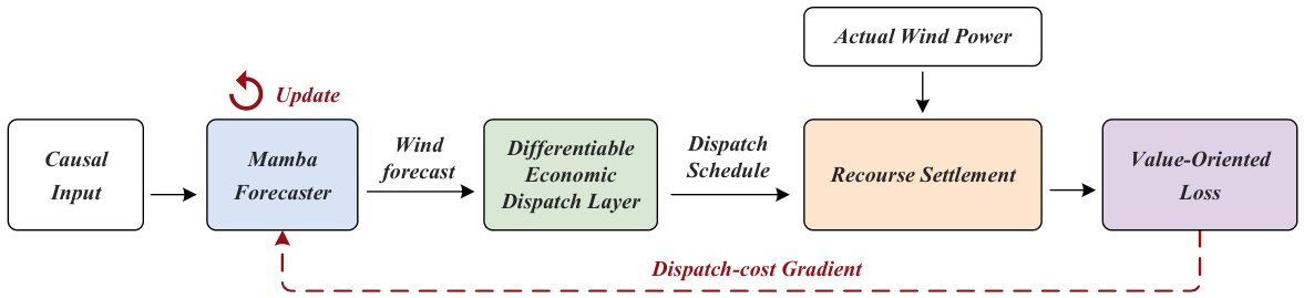
Figure 1 illustrates the proposed DVOF framework. At each forecast origin, the forecaster $f_{\theta }$ maps the causal information set ${\mathbf{c}}_t$ to a deterministic WPF ${\widehat{w}}_t$. The differentiable dispatch layer then solves the first-stage economic dispatch problem in Equations (3)–(5) using ${\widehat{w}}_t$, thereby determining the scheduled thermal generation $p^{★}\left({\widehat{w}}_t\right)$. Once the actual wind power $w_t$ is observed, the residual imbalance is settled through load shedding or wind curtailment, yielding the realized recourse cost $C^{\mathrm{rec}}({\widehat{w}}_t,w_t)$. Thus, $w_t$ is used to evaluate the forecast-induced schedule but is unavailable to the first-stage dispatch decision.

During training, the recourse-cost gradient is propagated from the settlement stage through the dispatch layer to the forecaster. The required sensitivity of the dispatch solution to the WPF is obtained primarily through KKT-based implicit differentiation, with a finite-difference fallback at numerically degenerate active-set configurations.

3.1. Mamba Forecaster

The wind-power forecaster $f_{\theta }$ maps a causal input $X\in {\mathbb{R}}^{T\times d_{\mathrm{in}}}$, which is the matrix form of the context ${\mathbf{c}}_t$, to a wind forecast $\widehat{w}$. The input has $d_{\mathrm{in}}=11$ features, and T denotes the number of tokens available at the forecast time. NWP variables are aligned with the target horizon. Each token contains historical wind power, six NWP variables (10 m and 100 m wind components $u,v$ and the derived wind speeds), and four calendar encodings (sin/cos of hour-of-day and day-of-year).

The mapping is implemented as a Mamba-style state-space sequence model (SSM) [15]. To make the architecture explicit, each module is denoted by a separate mapping function. The complete computation is

$$\begin{array}{cc}\hfill H^{\left(0\right)}& =F_{\mathrm{Embed}}\left(X\right)=F_L\left(X\right)+P_{\mathrm{pos}},\hspace{1em}\hfill \end{array}$$

(18)

$$\begin{array}{cc}\hfill H^{(\ell )}& =F_{\mathrm{M}}^{(\ell )}\left(H^{(\ell -1)}\right),\ell =1,\dots ,L,\hfill \end{array}$$

(19)

$$\begin{array}{cc}\hfill \overline{H}& =F_{\mathrm{LN}}\left(H^{\left(L\right)}\right),\hspace{1em}\hspace{1em}\hspace{1em}\hspace{1em}\hspace{1em}\hspace{1em}\hfill \end{array}$$

(20)

$$\begin{array}{cc}\hfill {\overline{h}}_T& ={\overline{H}}_T,\hspace{1em}\hspace{1em}\hspace{1em}\hspace{1em}\hspace{1em}\hspace{1em}\hspace{1em}\hspace{1em}\hfill \end{array}$$

(21)

$$\begin{array}{cc}\hfill \widehat{w}& =F_{\mathrm{out}}\left(F_{\mathrm{MLP}}\left({\overline{h}}_T\right)\right),\hspace{1em}\hspace{1em}\hspace{1em}\hspace{1em}\hfill \end{array}$$

(22)

where $F_L$ maps each $d_{\mathrm{in}}$-dimensional observation to a $d_{\mathrm{m}}$-dimensional token by a time-shared linear map applied to every row of X, $P_{\mathrm{pos}}\in {\mathbb{R}}^{T\times d_{\mathrm{m}}}$ denotes the learnable positional embedding, $F_{\mathrm{M}}^{(\ell )}$ denotes the ℓth Mamba-style selective-SSM block, and $F_{\mathrm{LN}}$ denotes layer normalization. The vector ${\overline{h}}_T$ is the representation of the last causal token. The forecasting head $F_{\mathrm{MLP}}$ comprises a linear layer, a GELU activation, and dropout, while $F_{\mathrm{out}}$ maps the resulting representation to the scalar wind-power forecast.

Selective-SSM Block

Let $H_{\mathrm{in}}\in {\mathbb{R}}^{T\times d_{\mathrm{m}}}$ denote the sequence entering one block. The block is written as a composition of six functions, namely, normalization, linear projection, local convolution, selective scan, gate modulation, and residual output.

A residual copy $R=H_{\mathrm{in}}$ is retained, and the input is normalized to $V=F_{\mathrm{LN}}\left(H_{\mathrm{in}}\right)$, which stabilizes the relative scale of the wind-power, NWP and calendar features before they enter the recurrent state update. The normalized sequence is then expanded and split into a candidate dynamics branch U and a gate branch Z,

$$[U,Z]=F_{\mathrm{in}}\left(V\right)=V{W}_{\mathrm{in}}^{\top }+\mathbf{1}{b}_{\mathrm{in}}^{\top },U,Z\in {\mathbb{R}}^{T\times d_{\mathrm{i}}},$$

(23)

where $W_{\mathrm{in}}\in {\mathbb{R}}^{2d_{\mathrm{i}}\times d_{\mathrm{m}}}$ and $b_{\mathrm{in}}\in {\mathbb{R}}^{2d_{\mathrm{i}}}$ are the weight and bias of the in-block projection, $\mathbf{1}\in {\mathbb{R}}^T$ is a vector of ones, and $d_{\mathrm{i}}$ is the expanded inner width. The candidate branch carries the temporal content to be propagated, whereas the gate branch controls how much of the resulting dynamic feature reaches the next layer.

The candidate branch is first processed by a causal depthwise convolution,

$$\tilde{U}=F_{\mathrm{SiLU}}\left(F_{\mathrm{Conv}.}\left(U\right)\right),$$

(24)

where $F_{\mathrm{Conv}.}$ applies a per-channel one-dimensional convolution of kernel width k with $k-1$ steps of left padding, so that each output position depends only on the current and preceding tokens, and $F_{\mathrm{SiLU}}$ is the sigmoid linear unit activation function.

The selective part of the block generates the SSM coefficients from the current token rather than using fixed coefficients for all hours, which is

$${\mathrm{\Delta }}_t=F_{\mathrm{\Delta }}\left({\tilde{u}}_t\right)=\mathrm{softplus}(W_{\mathrm{\Delta }}{\tilde{u}}_t+{\rho }_{\mathrm{\Delta }})+{\epsilon }_{\mathrm{\Delta }},{\mathit{\eta }}_t=F_B\left({\tilde{u}}_t\right),{\mathit{\xi }}_t=F_C\left({\tilde{u}}_t\right),$$

(25)

where ${\mathrm{\Delta }}_t\in {\mathbb{R}}^{d_{\mathrm{i}}}$, ${\mathit{\eta }}_t,{\mathit{\xi }}_t\in {\mathbb{R}}^N$ are the input-dependent state input and output projections, N is the latent state dimension, ${\rho }_{\mathrm{\Delta }}$ is the step bias, and ${\epsilon }_{\mathrm{\Delta }}={10}^{-4}$ is a small positive floor that keeps the step strictly positive. The symbols ${\mathit{\eta }}_t$ and ${\mathit{\xi }}_t$ replace the $B_t$ and $C_t$ of the standard selective-SSM notation, so that they are not confused with the generator cost coefficients $b_k$ and $C_k$ in Equation (2) or the context set ${\mathbf{c}}_t$ in Equation (1). With $A=-\exp \left(A_{\log }\right)\in {\mathbb{R}}^{d_{\mathrm{i}}\times N}$ and learned skip coefficient $D\in {\mathbb{R}}^{d_{\mathrm{i}}}$, the selective-SSM scan $Y=F_{\mathrm{Selective}-\mathrm{SSM}}\left(\tilde{U}\right)$ is computed channel-wise as

$$s_t^{\left(j\right)}=\exp \left({\mathrm{\Delta }}_t^{\left(j\right)}{A}^{\left(j\right)}\right)\odot s_{t-1}^{\left(j\right)}+{\mathrm{\Delta }}_t^{\left(j\right)}{\tilde{u}}_t^{\left(j\right)}{\mathit{\eta }}_t,o_t^{\left(j\right)}=〈{\mathit{\xi }}_t,s_t^{\left(j\right)}〉+D^{\left(j\right)}{\tilde{u}}_t^{\left(j\right)},$$

(26)

initialized by $s_0^{\left(j\right)}=0$, where $s_t^{\left(j\right)}\in {\mathbb{R}}^N$ is the latent state of channel j. The input-dependent step ${\mathrm{\Delta }}_t^{\left(j\right)}$ sets the memory length of that channel, so a block can hold a persistent wind state or discard it in favour of the current observation according to the token it is reading.

Finally, the scan output is modulated by the gate branch and projected back to the model width

$$\mathrm{\Gamma }=F_{\mathrm{SiLU}}\left(Z\right),Y_{\mathrm{g}}=Y\otimes \mathrm{\Gamma },H_{\mathrm{out}}=R+F_{\mathrm{Dropout}}\left(F_{\mathrm{BlockOut}}\left(Y_{\mathrm{g}}\right)\right),$$

(27)

where $\mathrm{\Gamma }$ is the gating signal, Y is the output of the selective scan, ⊗ is the element-wise product, $F_{\mathrm{BlockOut}}$ is the output projection of the block, and R restores the residual retained at its input.

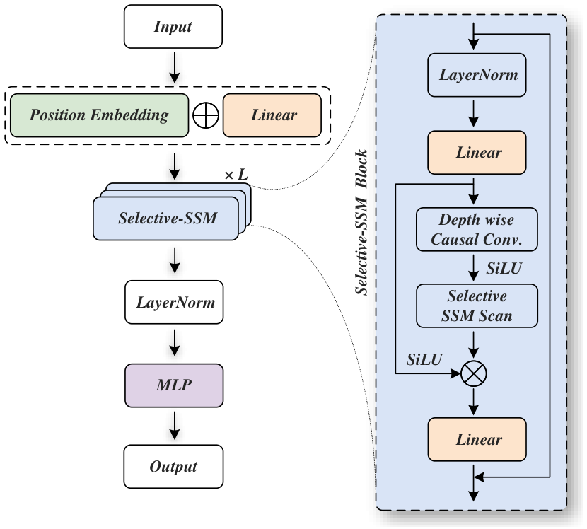
The complete architecture is summarized in Figure 2. Equations (18)–(22) define the overall forward path.

3.2. Differentiable Economic Dispatch Layer

To train $f_{\theta }$ through dispatch, Equations (3)–(5) are exposed as a layer $x^{★}\left(\widehat{w}\right)$. The forward pass solves the optimization problem, and the backward pass returns the sensitivity of the optimal solution to the wind forecast.

3.2.1. Forward Process

Collect the first-stage decision variables as $x=(p_1,\dots ,p_G,s^{\mathrm{curt}},s^{\mathrm{shed}})\in {\mathbb{R}}^{G+2}.$ For numerical differentiation, the implementation augments the first-stage objective with a small quadratic regularization term ${\epsilon }_s[{\left(s^{\mathrm{curt}}\right)}^2+{\left(s^{\mathrm{shed}}\right)}^2]$. The resulting regularized QP is

$$x^{★}\left(\widehat{w}\right)=\arg \underset{x}{\min }{\displaystyle \frac{1}{2}}{x}^{\top }Px+q^{\top }x\mathrm{s}.\mathrm{t}.A_{\mathrm{bal}}x=b\left(\widehat{w}\right),x^{\min }\le x\le x^{\max }\left(\widehat{w}\right),$$

(28)

where

$$\begin{array}{cccc}\hfill P& =\mathrm{diag}\left(2a_1,\dots ,2a_G,2{\epsilon }_s,2{\epsilon }_s\right),\hfill & \hfill q& =\left(b_1,\dots ,b_G,M^{\mathrm{plan}},M^{\mathrm{plan}}\right),\hfill \\ \hfill A_{\mathrm{bal}}& =(1,\dots ,1,-1,+1),\hfill & \hfill b\left(\widehat{w}\right)& =d-\widehat{w}.\hfill \end{array}$$

(29)

The box constraints collect the generator limits, $0\le s^{\mathrm{curt}}\le \widehat{w}$, and $0\le s^{\mathrm{shed}}\le d$. Because $a_k>0$ and ${\epsilon }_s>0$, the matrix P is positive-definite, and the regularized QP is strictly convex. The coefficient ${\epsilon }_s={10}^{-6}$ is used to stabilize differentiation while introducing only a small perturbation to the first-stage objective.

The forward QP is solved through CVXPY using the first available solver in the order ECOS, CLARABEL, OSQP, and SCS. In the computing environment used for the reported experiments, ECOS was unavailable, and CLARABEL was therefore used for all forward dispatch solves. The solver is used only to obtain the optimal first-stage solution, whereas gradients with respect to the WPF are computed separately through the KKT-based implicit-differentiation procedure described below. The scheduled thermal generation of Equation (6) is read from the first G coordinates of the stacked solution:

$$p^{★}\left(\widehat{w}\right)={\displaystyle \sum _{k=1}^G}{x}_k^{★}\left(\widehat{w}\right).$$

(30)

3.2.2. Backward Process by Implicit Differentiation

Let $\mathcal{A}$ denote the locally active set of box constraints at $x^{★}\left(\widehat{w}\right)$. Writing the box constraints in the canonical form $Ex\le h\left(\widehat{w}\right)$, where E collects the box-constraint rows and is distinct from the generator count G, the active constraints satisfy

$$E_{\mathcal{A}}{x}^{★}=h_{\mathcal{A}}\left(\widehat{w}\right).$$

(31)

Let $\nu \in \mathbb{R}$ and ${\lambda }_{\mathcal{A}}\ge 0$ denote the multipliers associated with the balance equation and active box constraints, respectively. The active-set KKT conditions are

$$\begin{array}{cc}\hfill P{x}^{★}+q+A_{\mathrm{bal}}^{\top }\nu +E_{\mathcal{A}}^{\top }{\lambda }_{\mathcal{A}}& =0,\hfill \\ \hfill A_{\mathrm{bal}}{x}^{★}& =b\left(\widehat{w}\right),\hfill \\ \hfill E_{\mathcal{A}}{x}^{★}& =h_{\mathcal{A}}\left(\widehat{w}\right).\hfill \end{array}$$

(32)

Under a locally unchanged active set and a nonsingular KKT system, differentiation with respect to $\widehat{w}$ gives

$$\underset{K}{\underbrace{\left[\begin{array}{ccc}P& A_{\mathrm{bal}}^{\top }& E_{\mathcal{A}}^{\top }\\ A_{\mathrm{bal}}& 0& 0\\ E_{\mathcal{A}}& 0& 0\end{array}\right]}}\left[\begin{array}{c}{\displaystyle \frac{\partial x^{★}}{\partial \widehat{w}}}\\ {\displaystyle \frac{\partial \nu }{\partial \widehat{w}}}\\ {\displaystyle \frac{\partial {\lambda }_{\mathcal{A}}}{\partial \widehat{w}}}\end{array}\right]=\left[\begin{array}{c}0\\ {\displaystyle \frac{\partial b}{\partial \widehat{w}}}\\ {\displaystyle \frac{\partial h_{\mathcal{A}}}{\partial \widehat{w}}}\end{array}\right].$$

(33)

Here, ${\displaystyle \frac{\partial b}{\partial \widehat{w}}}=-1$.

The vector $\partial h_{\mathcal{A}}/\partial \widehat{w}$ is zero except when the forecast-dependent upper bound $s^{\mathrm{curt}}\le \widehat{w}$ is active, in which case its corresponding entry equals one.

Because the training loss is scalar, the full solution Jacobian need not be formed. Let

$$g_x={\displaystyle \frac{\partial \mathcal{L}}{\partial x^{★}}}$$

(34)

denote the upstream gradient with respect to the dispatch solution. The system is assembled over the variables that are strictly inside their box constraints at $x^{★}$, because a variable held at a forecast-independent bound has zero local sensitivity. A diagonal term of ${10}^{-8}$ is added to K so that the factorization remains well posed. The adjoint vector $z=(z_x,z_{\nu },z_{\lambda })$ is obtained from

$$K^{\top }z=\left[\begin{array}{c}{g}_x\\ 0\\ 0\end{array}\right].$$

(35)

Then, the gradient with respect to the WPF is

$${\displaystyle \frac{\partial \mathcal{L}}{\partial \widehat{w}}}=z_{\nu }{\displaystyle \frac{\partial b}{\partial \widehat{w}}}+z_{\lambda }^{\top }{\displaystyle \frac{\partial h_{\mathcal{A}}}{\partial \widehat{w}}}=-z_{\nu }+z_{\lambda }^{\top }{\displaystyle \frac{\partial h_{\mathcal{A}}}{\partial \widehat{w}}}.$$

(36)

The second term of Equation (36) is written for the general case. Because the balance equation gives $s^{\mathrm{curt}}={\sum }_k{p}_k+\widehat{w}+s^{\mathrm{shed}}-d$, the bound $s^{\mathrm{curt}}\le \widehat{w}$ is attained only when the demand equals the minimum total thermal output. Whenever the demand is larger, the gradient reduces to $-z_{\nu }$, which is the case at every dispatch instance solved here.

3.2.3. Degeneracy Handling

The implicit-differentiation procedure may become unreliable when the active set changes or when the KKT matrix is singular or ill-conditioned. The layer therefore invokes the finite-difference fallback when the active-set construction is inconsistent, the condition number of K exceeds ${10}^{12}$, the factorization of K fails, or the resulting gradient is nonfinite or has a magnitude greater than ${10}^6$.

If any safeguard is triggered, the layer uses the central finite-difference approximation

$${\displaystyle \frac{\partial x^{★}}{\partial \widehat{w}}}\approx {\displaystyle \frac{x^{★}(\widehat{w}+ϵ)-x^{★}(\widehat{w}-ϵ)}{2ϵ}},ϵ={10}^{-3}\mathrm{p}.\mathrm{u}.$$

(37)

using two additional forward solves. The estimated solution Jacobian is then contracted with the upstream gradient $\partial \mathcal{L}/\partial x^{★}$.

Estimating the solution Jacobian rather than differentiating a particular downstream objective keeps the fallback applicable to the realized recourse cost in Equation (9). At active-set transitions, the finite-difference fallback provides a numerical directional approximation for stochastic optimization. The frequency of the fallback was measured over the training split for three of the matched seeds at both horizons. The exact KKT branch was used in $100.00\%$ of the $\mathrm{11,603}$ backward calls per seed at H = 24 and in at least $99.98\%$ of the $\mathrm{11,626}$ calls per seed at H = 1. The dispatch quadratic program is therefore well conditioned over the operating range visited in this study, and the reported gradients come from exact implicit differentiation.

3.3. Dispatch-Value-Oriented Training Objective

The network produces a raw normalized output ${\tilde{w}}_s$, where the subscript s marks a quantity expressed on the wind-power base $S_w$, which equals the wind rated power and is $1.0$ p.u. in the case study. Because the normalized wind power cannot exceed unity, the dispatch input is additionally capped at one. The non-negative prediction used in the accuracy term and the bounded dispatch input are defined, respectively, as

$${\widehat{w}}_s^{\mathrm{acc}}=\mathrm{ReLU}\left({\tilde{w}}_s\right),{\widehat{w}}_s^{\mathrm{disp}}=\min \{1,{\widehat{w}}_s^{\mathrm{acc}}\},\widehat{w}=S_w{\widehat{w}}_s^{\mathrm{disp}},w_s={\displaystyle \frac{w}{S_w}}.$$

(38)

The DVOF loss is

$$\mathcal{L}\left(\theta \right)=\underset{\mathrm{accuracy}\mathrm{term}}{\underbrace{{\left({\widehat{w}}_s^{\mathrm{acc}}-w_s\right)}^2}}+\beta \underset{\mathrm{normalized}\mathrm{recourse}\mathrm{term}}{\underbrace{{\displaystyle \frac{C^{\mathrm{rec}}(\widehat{w},w)}{M^{\mathrm{shed}}}}}},$$

(39)

where $C^{\mathrm{rec}}$ is defined in Equation (9). Division by $M^{\mathrm{shed}}$ controls the numerical scale of the recourse term, whereas $\beta$ determines its relative contribution to training.

Applying the chain rule through the differentiable dispatch layer gives

$${\displaystyle \frac{\partial \mathcal{L}}{\partial \theta }}=\underset{\mathrm{accuracy}\mathrm{term}}{\underbrace{2\left({\widehat{w}}_s^{\mathrm{acc}}-w_s\right){\displaystyle \frac{\partial {\widehat{w}}_s^{\mathrm{acc}}}{\partial \theta }}}}+{\displaystyle \frac{\beta }{M^{\mathrm{shed}}}}\underset{\mathrm{settlement}\mathrm{sensitivity}}{\underbrace{{\displaystyle \frac{\partial C^{\mathrm{rec}}}{\partial p^{★}}}}}\underset{\mathrm{dispatch}\mathrm{sensitivity}}{\underbrace{{\displaystyle \frac{\partial p^{★}}{\partial \widehat{w}}}}}{\displaystyle \frac{\partial \widehat{w}}{\partial \theta }}.$$

(40)

Away from the nondifferentiable point $n=d$, the settlement sensitivity is

$${\displaystyle \frac{\partial C^{\mathrm{rec}}}{\partial p^{★}}}=-M^{\mathrm{shed}}\mathbf{1}\{n<d\}+M^{\mathrm{curt}}\mathbf{1}\{n>d\},n=p^{★}\left(\widehat{w}\right)+w.$$

(41)

In the interior regime, scheduled thermal generation changes approximately one-for-one in the opposite direction to the WPF:

$${\displaystyle \frac{\partial p^{★}}{\partial \widehat{w}}}\approx -1.$$

(42)

Consequently, shortage hours generate a stronger conservative learning signal than curtailment hours when $M^{\mathrm{shed}}>M^{\mathrm{curt}}$. For the recourse-only component, the equilibrium of these asymmetric signals corresponds to the conditional quantile ${\tau }^{★}$ in Equation (14). Under the blended DVOF objective, the MSE term moderates this conservative shift.

3.4. Training Procedure

Algorithm 1 states the two-stage procedure: MSE pretraining, then DVOF fine-tuning from the checkpoint with the lowest validation MAE, with the recourse-cost gradient propagated through the dispatch layer. Two properties of the protocol are worth making explicit. The realized wind power $w_t$ never enters the forecaster input or the first-stage dispatch decision. It is the supervised target during training and validation and the reference realization at test time. Checkpoint selection also changes with the objective, from validation MAE in stage 1 to validation recourse cost in stage 2, so each arm is selected by the criterion it is meant to optimize.

Because each recourse evaluation requires a dispatch solve, the recourse term is applied to a uniformly spaced subset of mini-batches while the MSE term is applied to every one. This sparse evaluation approximates the blended objective of Equation (39), so $\beta$ is an empirically selected coefficient conditional on the adopted update frequency rather than a transferable constant.

Algorithm 1 Training of the proposed DVOF model

Require: Training set ${\mathcal{D}}_{\mathrm{tr}}$, validation set ${\mathcal{D}}_{\mathrm{val}}$, forecaster $f_{\theta }$, differentiable dispatch layer $\mathcal{G}$,   wind-power scale $S_w$, and trade-off coefficient $\beta$. Ensure: Best MSE model ${\theta }^{\mathrm{MSE}}$ and best DVOF model ${\theta }^{\mathrm{DVOF}}$. 1: Stage 1: MSE pretraining 2: Initialize $\theta$ 3: for each pretraining epoch do 4:    for each mini-batch $\mathcal{B}\subset {\mathcal{D}}_{\mathrm{tr}}$ do 5:      Compute ${\tilde{w}}_{s,t}=f_{\theta }\left({\mathbf{c}}_t\right)$, ${\widehat{w}}_{s,t}^{\mathrm{acc}}=\mathrm{ReLU}\left({\tilde{w}}_{s,t}\right)$, ${\widehat{w}}_{s,t}^{\mathrm{disp}}=\min \{1,{\widehat{w}}_{s,t}^{\mathrm{acc}}\}$, and ${\widehat{w}}_t=S_w{\widehat{w}}_{s,t}^{\mathrm{disp}}$ 6:      Compute $w_{s,t}=w_t/S_w$ 7:      Compute ${\mathcal{L}}_{\mathrm{MSE}}={\displaystyle \frac{1}{\left|\mathcal{B}\right|}}{\sum }_{t\in \mathcal{B}}{({\widehat{w}}_{s,t}^{\mathrm{acc}}-w_{s,t})}^2$ 8:      Update $\theta$ using ${\nabla }_{\theta }{\mathcal{L}}_{\mathrm{MSE}}$ 9:    end for 10:  Evaluate validation MAE and save the checkpoint if it improves 11: end for 12: Restore the checkpoint with the lowest validation MAE 13: Set ${\theta }^{\mathrm{MSE}}\leftarrow \theta$ 14: Stage 2: DVOF fine-tuning 15: Initialize $\theta \leftarrow {\theta }^{\mathrm{MSE}}$ 16: Select a uniformly spaced subset of mini-batches ${\mathcal{B}}_{\mathrm{dec}}$ for recourse-loss evaluation 17: for each fine-tuning epoch do 18:    for each mini-batch $\mathcal{B}\subset {\mathcal{D}}_{\mathrm{tr}}$ do 19:      Compute ${\tilde{w}}_{s,t}=f_{\theta }\left({\mathbf{c}}_t\right)$, ${\widehat{w}}_{s,t}^{\mathrm{acc}}=\mathrm{ReLU}\left({\tilde{w}}_{s,t}\right)$, ${\widehat{w}}_{s,t}^{\mathrm{disp}}=\min \{1,{\widehat{w}}_{s,t}^{\mathrm{acc}}\}$, and ${\widehat{w}}_t=S_w{\widehat{w}}_{s,t}^{\mathrm{disp}}$ 20:      Compute $w_{s,t}=w_t/S_w$ 21:      Compute ${\mathcal{L}}_{\mathrm{MSE}}={\displaystyle \frac{1}{\left|\mathcal{B}\right|}}{\sum }_{t\in \mathcal{B}}{({\widehat{w}}_{s,t}^{\mathrm{acc}}-w_{s,t})}^2$ 22:      if $\mathcal{B}\in {\mathcal{B}}_{\mathrm{dec}}$ then 23:         Obtain $p_t^{★}=\mathcal{G}({\widehat{w}}_t,d_t)$ and compute $C_t^{\mathrm{rec}}({\widehat{w}}_t,w_t)$ 24:         Set $\mathcal{L}={\mathcal{L}}_{\mathrm{MSE}}+{\displaystyle \frac{\beta }{\left|\mathcal{B}\right|}}{\sum }_{t\in \mathcal{B}}{C}_t^{\mathrm{rec}}({\widehat{w}}_t,w_t)/M^{\mathrm{shed}}$ 25:      else 26:         Set $\mathcal{L}={\mathcal{L}}_{\mathrm{MSE}}$ 27:      end if 28:      Update $\theta$ using ${\nabla }_{\theta }\mathcal{L}$ 29:    end for 30:    Evaluate validation recourse cost and save the checkpoint if it improves 31: end for 32: Restore the checkpoint with the lowest validation recourse cost 33: Set ${\theta }^{\mathrm{DVOF}}\leftarrow \theta$ 34: return ${\theta }^{\mathrm{MSE}}$ and ${\theta }^{\mathrm{DVOF}}$

4. Experimental Results and Discussion

4.1. Experimental Setup

4.1.1. Data and Evaluation Metrics

The forecasting data are drawn from Zone 3 of the GEFCom2014 wind track, which contains hourly normalized wind-power observations and numerical weather prediction (NWP) variables [31]. At each forecast origin, the causal input sequence combines observed historical wind power, horizon-aligned NWP information, and sine–cosine calendar encodings for hour of day and day of year. The data are divided chronologically, without shuffling, into training, validation, and test segments in the ratio $0.70/0.15/0.15$, corresponding to $\mathrm{11,698}$, 2506, and 2508 h, respectively. The evaluation considers one-hour-ahead (H = 1) and day-ahead (H = 24) forecasts.

The demand shape is obtained from Zone 1 of the GEFCom2014 load track. Because the public wind and load tracks span different calendar periods, the load series is aligned to the wind calendar from a common January origin and paired hour by hour. The resulting demand profile defines a standardized dispatch scenario rather than an observed joint wind–load trajectory. Consequently, the case study isolates the forecast–dispatch mechanism under a controlled demand shape, and it does not reproduce the temporal co-movement of a particular power system. Validation using contemporaneous wind and load measurements is required before operational generalization. Let $e_t={\widehat{w}}_t-w_t$ denote the signed forecast error over the N test samples. Forecasting performance is evaluated using the MAE, RMSE and $R^2$ in their standard definitions, where lower MAE and RMSE and higher $R^2$ indicate better statistical accuracy. The signed error is reported as a distribution rather than as a single bias value, because its location relative to zero is the quantity that carries operational meaning. A forecast displaced below the realization is conservative, and shortage and surplus incur asymmetric recourse penalties.

Dispatch value is evaluated by settling every forecast through the schedule-then-recourse procedure in Section 2. The primary value metric is the realized imbalance penalty, $M^{\mathrm{shed}}\mathrm{shed}+M^{\mathrm{curt}}\mathrm{curt}$, because it is the recourse cost induced directly by the forecast-based generation schedule.

For each seed, all eligible timestamps in the held-out chronological test segment are settled before the seed-level metrics are calculated. The comparison of loss-defined models uses the six matched seeds $\{0,11,22,33,44,55\}$, so that every model sees an identical set of initializations and paired comparisons are available. The penalty-ratio and $\beta$ studies of Section 4.3.5 require a separate training run per scenario point and use the three matched seeds $\{0,11,22\}$, as their captions state. The resulting dispersion characterizes sensitivity to initialization within the present data and scenario and does not establish robustness to distribution shift or alternative market designs.

4.1.2. Compared Models and Experimental Configuration

The benchmarks are organized in two stages, which separates the choice of forecasting backbone from the choice of training objective. First, the Mamba-style forecaster is compared with persistence, LSTM, GRU, Transformer and DLinear to establish the statistical competence of the selected backbone, and all learned models share the causal input of Section 4.1.1, the Adam optimizer, gradient clipping and early stopping on validation MAE. Second, the architecture is held fixed and only the objective is varied across the four loss-defined models below, which together separate the contribution of statistical accuracy, of a cost-aware conservative shift, and of the differentiable dispatch layer itself.

MSE Loss model. This accuracy-oriented model is trained using MSE and selected using validation MAE. As an estimate of the conditional mean, it provides the principal statistical baseline for evaluating whether DVOF training can reduce realized imbalance penalty.

Pinball Loss model, fixed $\tau$= 2/9. This quantile-regression model uses the same backbone and is trained with the pinball loss. Its dispatch quantile is fixed at $\tau$= 2/9, the value adopted in the related value-oriented forecasting formulation [17]. It is retained for comparability with that work and is not presented as the optimal quantile of the present scenario.

Pinball Loss model, validation selected. This control uses the same quantile-regression backbone but chooses its dispatch quantile per seed from the candidate set $\{0.05,0.0909,0.10,1/6,2/9,0.30,0.50\}$ by minimizing the realized imbalance penalty on the validation split. The test split is never used in the selection. Because it locates the cost-optimal quantile by direct search under the operative recourse scenario, it is the strongest control available to a forecaster that does not differentiate through the dispatch problem, and it is the reference against which the incremental contribution of the dispatch layer is judged.

Proposed DVOF Loss model. This model starts from the MSE-trained forecaster and is fine-tuned using Equation (39), which combines MSE with a differentiable recourse-cost term. It receives no quantile level and performs no search over one.

Table 1. Main hyperparameters and selection protocol of the MSE-trained Mamba-style forecaster.

Group	Hyperparameter	Value	Candidates
Input	Historical context length	72 h	$\{12,24,48,72\}$
	Forecast horizon H	1/24 h	-
Mamba SSM	Model dimension	96	$\{32,64,96,128\}$
	Number of SSM layers	3	$\{1,2,3\}$
	State dimension	16	$\{8,16,32\}$
	Convolution width	7	$\{3,4,5,7\}$
	Expansion factor	2	$\{1,2,3\}$
Training	Dropout	0.2740	$[0,0.3]$
	Optimizer	Adam	-
	Learning rate	$9.40\times {10}^{-4}$	$[{10}^{-4},3\times {10}^{-3}]$
	Weight decay	$4.12\times {10}^{-5}$	$[{10}^{-7},{10}^{-3}]$
	Batch size	256	$\{128,256,512\}$

reports the backbone and its selection protocol. A 50-trial Optuna study, of which 47 completed, was run on the one-hour-ahead MSE-trained forecaster and ranked by validation MAE under the chronological training–validation split. The searched variables and their candidate ranges are listed beside every selected value. The resulting architecture was then fixed for all four loss-defined models at both horizons, with DVOF fine-tuning using its objective-specific optimization schedule. Because the selection criterion is validation MAE, dispatch-cost information does not enter the choice of backbone and no arm of the comparison is tuned preferentially.

The dispatch environment is deliberately simplified so that the effect of asymmetric recourse on the forecasting gradient can be identified. It retains power balance, continuous generation-output bounds, and non-negative load-shedding and wind-curtailment recourse, while omitting network power flows, intertemporal ramping, reserve procurement, storage dynamics, multi-area exchanges, and binary commitment decisions. Holding these coupled effects outside the model separates the forecast adjustment induced by the recourse asymmetry from adjustments attributable to a particular network or intertemporal constraint. Accordingly, the supplementary scenario analysis changes the recourse-cost ratio only and holds the remaining operating conditions fixed. The model is therefore used to study the forecast–decision mechanism under controlled conditions, rather than to reproduce the market design of a specific control area. The configuration of the economic-dispatch test system is shown in

Table 2. Two-unit economic-dispatch test system configuration (per unit on the wind rated power).

Thermal Unit	${\mathit{p}}^{\min }$ (p.u.)	${\mathit{p}}^{\max }$ (p.u.)	a (c.u./p.u.2h)	b (c.u./p.u. h)
T1	0	0.80	12	30
T2	0	0.50	15	35

Peak load $1.6$ p.u.; wind rated power $1.0$ p.u.; no PV. Stylized recourse penalties $M^{\mathrm{shed}}=1000$, $M^{\mathrm{curt}}=100$ c.u./p.u. h (ratio $10:1$).

.

4.2. Forecasting Competence of the Mamba Backbone

The forecasting backbone is first evaluated independently of the dispatch objective. A value-oriented training objective is informative only when it is applied to a statistically competitive forecaster. Figure 3 and

Table 3. Forecasting accuracy of the proposed Mamba forecaster against standard deep-learning baselines and the persistence reference. Values are the mean ± standard deviation over six random seeds. The best MAE, RMSE, and $R^2$ values in each horizon are shown in bold. Bias is reported as a signed diagnostic.

Horizon	Model	MAE	RMSE	${\mathit{R}}^2$	Bias
H = 1	Persistence	0.0731	0.1066	0.881	0.0001
	LSTM [8]	0.0664 ± 0.0004	0.0927 ± 0.0007	0.910 ± 0.001	$0.0034\pm 0.0027$
	GRU [9]	0.0661 ± 0.0005	0.0930 ± 0.0005	0.909 ± 0.001	$0.0001\pm 0.0038$
	Transformer [13]	0.0673 ± 0.0009	0.0941 ± 0.0008	0.907 ± 0.002	$0.0087\pm 0.0060$
	DLinear [14]	0.0990 ± 0.0205	0.1237 ± 0.0247	0.834 ± 0.074	$-0.0105\pm 0.0070$
	Proposed	0.0657 ± 0.0011	0.0921 ± 0.0011	0.911 ± 0.002	$0.0048\pm 0.0096$
H = 24	Persistence	0.3364	0.4150	$-0.813$	0.0027
	LSTM [8]	0.1127 ± 0.0013	0.1479 ± 0.0012	0.770 ± 0.004	$0.0166\pm 0.0129$
	GRU [9]	0.1143 ± 0.0016	0.1508 ± 0.0014	0.761 ± 0.005	$0.0250\pm 0.0086$
	Transformer [13]	0.1144 ± 0.0017	0.1515 ± 0.0030	0.758 ± 0.010	$0.0245\pm 0.0137$
	DLinear [14]	0.1285 ± 0.0014	0.1593 ± 0.0020	0.733 ± 0.007	$-0.0170\pm 0.0036$
	Proposed	0.1105 ± 0.0022	0.1459 ± 0.0023	0.776 ± 0.007	$0.0132\pm 0.0113$

therefore compare the Mamba-style backbone with the learned baselines and the persistence reference.

All learned models are trained under the same causal-input and MSE-training protocol and are evaluated across six random initializations. Table 3 reports the resulting accuracy metrics, and Figure 3 provides an illustrative trajectory from the held-out test segment.

The purpose of this comparison is to establish that the selected backbone is a competitive predictor, so that the subsequent comparison of training objectives is not confounded by a weak forecaster. It is not to claim architectural superiority. Table 3 shows that the Mamba-style forecaster attains the lowest mean MAE and RMSE and the highest mean $R^2$ at both horizons, but the margin over the strongest learned baselines is within the seed-to-seed dispersion. At H = 24, its MAE is $2.0\%$ below LSTM, a difference of about one pooled standard error over six seeds, and at H = 1, it is $0.6\%$ below GRU, well inside the dispersion. Neither gap is statistically separated, and the appropriate conclusion is that the Mamba-style backbone performs on par with the strongest recurrent baselines rather than better than them.

The differences that are unambiguous lie elsewhere. All learned models improve substantially on persistence at the day-ahead horizon, where the MAE and RMSE fall by $67.2\%$ and $64.8\%$, and the $R^2$ rises from $-0.813$ to $0.776$; and all outperform DLinear, whose MAE is $14.0\%$ higher at H = 24 and whose seedwise dispersion at $H=1$ is an order of magnitude larger than that of the other learned models. The signed bias of every accuracy-trained model is small. The backbone is therefore adequate for the purpose at hand, and the results of Section 4.3 can be attributed to the training objective rather than to the choice of architecture.

The representative trajectories in Figure 3 are consistent with the aggregate results. The Mamba-style forecast follows the principal ramps in the displayed interval, whereas persistence exhibits the expected horizon-dependent lag and misses several ramp onsets. The figure is illustrative, and the quantitative comparison and its variability across seeds are reported in Table 3.

4.2.1. Computational Cost

Computational efficiency is evaluated under an identical input and hardware configuration for all backbones. Timings are averaged over repeated runs on an NVIDIA GeForce RTX 5070 Ti GPU using PyTorch 2.13 and CUDA 13.2. Latency is reported per sample, calculated as batch time divided by batch size, at T = 72.

Table 4. Computational cost of the compared backbones under the same input configuration (T = 72).

Model	Parameters	Inference ($\mathsf{\mu }$s/Sample)	Training ($\mathsf{\mu }$s/Sample)
LSTM [8]	≈116 $\mathrm{k}$	$2.3$	$6.7$
GRU [9]	≈87 $\mathrm{k}$	$2.0$	$6.5$
Transformer [13]	≈158 $\mathrm{k}$	$4.8$	$22.0$
DLinear [14]	≈1.4 $\mathrm{k}$	$0.8$	$4.5$
Proposed	≈330 $\mathrm{k}$	$88.4$	$424.5$

reports the number of trainable parameters and the inference and training latencies. The Mamba-style forecaster contains approximately $330\mathrm{k}$ trainable parameters, about 2.1 times the Transformer size and 3.8 times the GRU size. Its inference and training latencies are $88.4$ and $424.5\mathsf{\mu }\mathrm{s}$/sample, respectively. Thus, at the context length used in the main experiments, the proposed backbone does not offer a latency advantage over the alternative models.

One qualification is essential to interpreting these timings. The selective scan is implemented in plain PyTorch as an explicit recurrence over the T time steps, so that the model runs without the fused CUDA kernels of the original Mamba implementation. The measured latency therefore reflects a reference implementation with a large per-step constant rather than an intrinsic property of the selective-SSM architecture, and it should not be read as a like-for-like comparison against the highly optimized fused kernels behind the recurrent and attention baselines. What the measurements do establish is the scaling behavior of the selective scan, which is linear in T as the architecture predicts, and the absolute cost of the configuration actually used in this study.

The choice of backbone therefore reflects a trade-off among statistical accuracy, realized recourse value and computational demand rather than a preference for model complexity. In the present use case, the trade-off is not binding, because the absolute inference time stays below $0.1$ ms/sample at T = 72, which is negligible against the one-hour and day-ahead decision horizons, and training and DVOF fine-tuning are offline and do not enter the online execution time after deployment.

Selective scanning has linear sequence-length complexity, whereas standard self-attention has quadratic complexity, but no latency crossover is observed between T = 24 and T = 768, because the per-step constant of the reference implementation dominates at these context lengths. The measured growth rates are nonetheless the ones the two complexity classes predict once the sequence is long enough that fixed overheads no longer dominate. Over T = 192 to 768, the proposed model slows by a factor of $4.0$ for a fourfold increase in T, whereas the Transformer slows by a factor of $7.3$. Below T = 192, the comparison is governed by constant terms rather than by asymptotic order. The proposed backbone is therefore selected for its forecasting and dispatch behavior rather than for execution speed at the studied context length.

Three routes are available to a deployment-oriented study, and they act on different parts of the cost. The first is to replace the reference scan with the fused selective-scan kernel, which removes the per-step Python 3.14 overhead identified above and is expected to give the largest single reduction without changing the model. The second is structured pruning of the width parameters that dominate the parameter count, namely, the state dimension N and the expansion factor, together with post-training quantization of the linear projections, both of which reduce memory traffic in the recurrence. The third is knowledge distillation of the trained forecaster into a smaller recurrent or linear student, which is attractive here because the deployed artefact is a deterministic point forecaster and the DVOF objective is applied only during offline fine-tuning. A distilled student would nevertheless have to be re-checked against the operating-point diagnostics of Section 4.3.1, since compression that preserves MAE does not automatically preserve the attained quantile level that determines dispatch value.

4.2.2. Backbone-Selection Sensitivity

Figure 4 summarizes the completed Optuna study. The functional analysis of variance (fANOVA) diagnostic estimates that weight decay and model dimension account for $55.7\%$ and $24.0\%$, respectively, of the normalized relative importance for validation MAE within the sampled search space. The remaining hyperparameters have lower marginal importance. This ranking is conditional on the trial distribution and parameter interactions and should not be interpreted as a causal decomposition. Its role is to document the stability of backbone selection, not to infer sensitivity of realized recourse cost.

4.3. Evaluation of the Proposed DVOF Framework

The evaluation proceeds in three steps. Section 4.3.1 establishes where each training objective places the forecast by measuring the quantile level the forecast attains and comparing it with the level implied by the recourse model. Section 4.3.3 quantifies what that placement costs against an accuracy-oriented control and a cost-aware quantile control, and Section 4.3.5 examines how both results respond to the recourse scenario and to the training weight. Unless stated otherwise, the configuration is $M^{\mathrm{shed}}:M^{\mathrm{curt}}=10:1$ with $\beta =35$, and all values are test-set results over the six matched seeds $\{0,11,22,33,44,55\}$.

Two quantile controls are used throughout and are kept distinct. The fixed control uses $\tau =2/9$, the value inherited from the related value-oriented forecasting formulation [17] and is retained for comparability with that work rather than as an optimum for the present scenario. The validation-selected control chooses $\tau$ separately for each seed from the candidate set $\{0.05,0.0909,0.10,1/6,2/9,0.30,0.50\}$ using validation imbalance penalty only and is therefore the stronger benchmark.

4.3.1. Attained Operating Point of the Trained Forecasts

Equation (14) identifies the recourse-optimal forecast as the conditional ${\tau }^{★}$-quantile of wind power, with ${\tau }^{★}=0.0909$ under the nominal penalty ratio. This closed form admits a direct test of whether the differentiable layer transmits the intended economic signal. The quantile level that a trained forecast attains is measurable on the test set as the empirical frequency $\mathrm{Pr}(w\le \widehat{w})$ and can be compared with ${\tau }^{★}$. The measurement requires no quantile supervision and applies equally to point and quantile forecasters.

Table 5. Quantile level attained by each trained forecast on the test split, measured as $\mathrm{Pr}(w\le \widehat{w})$. The recourse-optimal level under the nominal $10:1$ ratio is ${\tau }^{★}=0.0909$. Values are mean over the six matched seeds $\{0,11,22,33,44,55\}$, with the seedwise range in brackets.

Model	H = 1	H = 24
MSE Loss	$0.530$$[0.478,0.606]$	$0.539$$[0.493,0.595]$
Pinball Loss, fixed $\tau$ = 2/9 [17]	$0.245$$[0.187,0.289]$	$0.240$$[0.205,0.263]$
Pinball Loss, validation selected	$0.149$$[0.115,0.181]$	$0.166$$[0.130,0.197]$
Proposed DVOF Loss	$0.135$$[0.114,0.180]$	$0.164$$[0.146,0.182]$

Recourse-optimal reference ${\tau }^{★}=M^{\mathrm{curt}}/(M^{\mathrm{shed}}+M^{\mathrm{curt}})=0.0909$.

reports the result. The MSE Loss model operates near the conditional median, at $0.530$ and $0.539$, as expected for an estimator of the conditional mean. The Proposed DVOF Loss model operates at $0.135$ and $0.164$, having moved most of the distance from the median toward ${\tau }^{★}$. It reaches this operating point from the dispatch gradient alone, without being supplied with a quantile level and without any search over $\tau$. The validation-selected Pinball Loss model, which reaches its operating point by an explicit seven-point search on the validation split, settles at the closely similar levels $0.149$ and $0.166$. The fixed $\tau$= 2/9 control stops short of both, at $0.245$ and $0.240$, which is the expected consequence of importing a quantile calibrated for a different penalty ratio.

The agreement between an end-to-end trained point forecaster and an explicitly tuned quantile forecaster indicates that the KKT-based gradient of Section 3.2 carries the asymmetry of the recourse model faithfully enough to recover the economically correct operating point without supervision. Both learned levels remain above ${\tau }^{★}$ for two reasons. The blended objective of Equation (39) retains an MSE term that moderates the conservative shift, and the generator bounds truncate the interior solution on which Equation (14) is derived.

4.3.2. Stability of the Operating Point Across Operating Conditions

Equation (14) further shows that ${\tau }^{★}$ depends only on the penalty ratio and not on the weather regime. A value-oriented forecaster should therefore hold a condition-independent operating point, whereas a forecaster that fixes a quantile of the conditional distribution need not, because the same probability level maps to different economic positions as the conditional spread changes. This provides a second and sharper test of the differentiable layer.

The held-out period is stratified by terciles of the horizon-aligned 100 m NWP wind speed. This variable is available at the forecast origin and is independent of the realized wind power, so the stratification cannot induce a selection artefact.

Table 6. Attained quantile level $\mathrm{Pr}(w\le \widehat{w})$ within terciles of the horizon-aligned 100 m NWP wind speed, a conditioning variable known at the forecast origin. Spread is the range across the three strata. Values are means over the six matched seeds $\{0,11,22,33,44,55\}$.

Model	H = 1				H = 24
	Low	Mid	High	Spread	Low	Mid	High	Spread
MSE Loss	$0.551$	$0.563$	$0.477$	$0.086$	$0.578$	$0.558$	$0.483$	$0.095$
Pinball, fixed $\tau$ = 2/9	$0.319$	$0.225$	$0.190$	$0.130$	$0.290$	$0.245$	$0.187$	$0.104$
Pinball, validation selected	$0.204$	$0.135$	$0.108$	$0.097$	$0.199$	$0.176$	$0.123$	$0.075$
Proposed DVOF Loss	$0.166$	$0.123$	$0.117$	$0.048$	$0.178$	$0.171$	$0.143$	$0.035$

reports the attained quantile level within each stratum. The Proposed DVOF Loss model varies by $0.048$ at H = 1 and $0.035$ at H = 24 across the three strata, whereas every control varies more. The fixed-$\tau$ control drifts from $0.319$ in low wind to $0.190$ in high wind at H = 1, a spread of $0.130$, and the validation-selected control spreads by $0.097$ and $0.075$.

Because each seed supplies a matched observation of every model, the comparison can be made pairwise. At H = 24, the Proposed DVOF Loss model has the smaller spread in all six seeds against each of the three controls, and the paired differences are statistically separated, with $\left|t\right|$ between $3.44$ and $5.65$ against a critical value of $2.57$. At H = 1, it has the smaller spread in five of six seeds against each control, with $\left|t\right|$ between $2.02$ and $2.95$, so the ordering is consistent but separated only against the fixed-$\tau$ control. The distinction is one of the quantity being held fixed. A quantile head equalizes a probability level, whereas the dispatch gradient equalizes the marginal economic trade-off, and it is the latter that Equation (14) identifies as constant across operating conditions.

4.3.3. Realized Dispatch Cost Against the Accuracy and Quantile Controls

Table 7. Dispatch-value comparison of the four loss-defined models on the identical Mamba backbone. Both quantile controls are shown: the fixed reference $\tau$ = 2/9 and the validation-selected quantile.

H	Model	Penalty	MAE	${\mathbf{\Delta }}_{\mathbf{MSE}}$	${\mathbf{\Delta }}_{\mathbf{Q}}$
H = 1	MSE loss	$35.02\pm 3.07$	$\mathbf{0.066}$	—	—
	Pinball loss, fixed $\tau$ = 2/9 [17]	$20.59\pm 1.33$	$0.084$	$-41.2\%$	—
	Pinball loss, validation selected	$18.42\pm 0.48$	$\mathbf{0.105}$	$-47.4\%$	—
	Proposed DVOF loss	$\mathbf{18.29}\pm \mathbf{0.27}$	$0.106$	$-\mathbf{47.8}\%$	$-0.7\%$
H = 24	MSE loss	$55.47\pm 4.05$	$\mathbf{0.111}$	—	—
	Pinball loss, fixed $\tau$ = 2/9 [17]	$29.47\pm 1.25$	$0.139$	$-46.9\%$	—
	Pinball loss, validation selected	$\mathbf{26.11}\pm \mathbf{0.84}$	$\mathbf{0.165}$	$-\mathbf{52.9}\%$	—
	Proposed DVOF loss	$26.59\pm 1.02$	$0.167$	$-52.1\%$	$+1.9\%$

Values are mean ± two-sided $95\%$ confidence interval over the six matched seeds $\{0,11,22,33,44,55\}$. Penalty is the realized imbalance penalty under schedule-then-recourse dispatch and is reported in c.u. ${\mathrm{h}}^{-1}$. ${\mathrm{\Delta }}_{\mathrm{MSE}}$ and ${\mathrm{\Delta }}_{\mathrm{Q}}$ are measured against the MSE and validation-selected Pinball Loss models, respectively. Bold face denotes the numerical minimum.

first establishes the forecast–decision mismatch that motivates DVOF. From the table, the MSE Loss model attains the lowest MAE but the highest realized imbalance penalty at both horizons. Relative to this accuracy-oriented reference, the Proposed DVOF Loss model reduces the mean penalty by $47.8\%$ at H = 1 and $52.1\%$ at H = 24, while accepting a larger MAE and a more negative error location. The validation-selected Pinball Loss model then provides the relevant cost-aware comparison. Its mean penalty is close to that of DVOF at H = 1 ($18.42$ and $18.29$ c.u. ${\mathrm{h}}^{-1}$, respectively) and lower at H = 24 ($26.11$ vs. $26.59$ c.u. ${\mathrm{h}}^{-1}$). The paired six-seed comparison detects no significant difference at either horizon ($\left|t\right|$ = 1.06 and $1.12$, respectively). The two methods nevertheless arrive at these outcomes differently. The Pinball model selects a quantile from a validation bank, whereas DVOF obtains its forecast adjustment from the dispatch gradient without prescribing a quantile level.

Table 8. Seedwise distribution of realized imbalance penalty in the controlled test scenario. Values summarize the same three matched runs used in Table 7.

H	Model	Minimum	Maximum	SD
1	MSE Loss	$30.74$	$37.82$	$2.93$
	Pinball Loss ($\tau$ = 2/9)	$18.85$	$22.72$	$1.27$
	Pinball Loss (validation selected)	$18.00$	$19.29$	$0.46$
	Proposed DVOF Loss	$18.03$	$18.72$	$0.26$
24	MSE Loss	$51.01$	$61.52$	$3.86$
	Pinball Loss ($\tau$ = 2/9)	$27.37$	$30.57$	$1.19$
	Pinball Loss (validation selected)	$24.82$	$27.14$	$0.80$
	Proposed DVOF Loss	$25.61$	$28.01$	$0.97$

gives the seedwise distribution behind these means. Figure 5 decomposes the penalty into its physical parts and is discussed in Section 4.3.6.

Figure 6 reports the distribution of the signed forecast error itself, pooled over the matched seeds and the complete held-out set, and identifies what the value-oriented objective changes and what it leaves alone. The standard deviation is nearly common to all four models, at $0.092$ to $0.098$ at H = 1 and $0.145$ to $0.153$ at H = 24, so the training objective does not measurably alter the sharpness of the forecast. What moves is the location. The whole distribution is displaced downward, with the median falling from $+0.003$ to $-0.087$ at H = 1 and from $+0.009$ to $-0.139$ at H = 24. This is the signature of a quantile shift rather than of an improvement in predictive skill, and it is the distributional counterpart of the attained levels in Table 5. The left panel of Figure 7 shows the weekly aggregation of the realized penalty over the whole held-out period.

4.3.4. Event-Conditioned Evaluation

An aggregate mean can conceal the hours that matter operationally. The held-out period is therefore partitioned by rules fixed before any test result was examined. High-ramp hours are those whose realized wind change $|w_t-w_{t-1}|$ reaches the 90th percentile of the same statistic on the training split, a threshold of $0.1516$ p.u., which selects 305 of the 2508 test h. High-imbalance hours are those whose realized recourse under the accuracy-oriented MSE reference reaches its 90th test percentile, which selects 251 h. The high-imbalance partition is derived once from the reference model and applied unchanged to every model, so all models are scored on a common set of hours.

Table 9. Event-conditioned mean imbalance penalty (c.u. ${\mathrm{h}}^{-1}$) over the six matched seeds $\{0,11,22,33,44,55\}$. Strata are defined by rules fixed before the test results were examined. Hour counts are given in the header.

H	Model	All Hours	High Ramp	High Imbalance
		(2508 h)	(305 h)	(251 h)
H = 1	MSE Loss	$35.02$	$76.84$	$147.30$
	Pinball, fixed $\tau$ = 2/9	$20.59$	$53.68$	$71.48$
	Pinball, validation selected	$18.42$	$46.00$	$47.71$
	Proposed DVOF Loss	$18.29$	$45.92$	$44.98$
H = 24	MSE Loss	$55.47$	$77.13$	$240.25$
	Pinball, fixed $\tau$ = 2/9	$29.47$	$46.18$	$105.76$
	Pinball, validation selected	$26.11$	$39.80$	$70.91$
	Proposed DVOF Loss	$26.59$	$40.34$	$74.75$

examines whether the aggregate result persists when the dispatch is stressed. The MSE Loss model remains the highest-penalty model in every stratum, and the gap between the accuracy-oriented and cost-aware objectives widens markedly in high-imbalance hours. For example, at H = 24, its mean penalty rises to $240.25$ c.u. ${\mathrm{h}}^{-1}$, compared with $74.75$ for DVOF, whereas the corresponding all-hours values are $55.47$ and $26.59$ c.u. ${\mathrm{h}}^{-1}$.

Within the cost-aware comparison, the horizon-dependent ordering in Table 7 is retained. DVOF has the lower mean penalty in all H = 1 strata, whereas the validation-selected Pinball model is lower in every H = 24 stratum. Thus, the aggregate comparison is not driven by the inclusion of undemanding hours. At H = 1, ramp events remain the most difficult stratum for all four models, consistent with the reduced value of persistence information during rapid wind changes.

4.3.5. Sensitivity to the Recourse Scenario and the Training Weight

Two quantities are varied here and must not be confused. The penalty ratio is a property of the operating environment and changes the recourse gradient itself. The trade-off weight $\beta$ is a property of the training objective in Equation (39) and changes how strongly the forecaster responds to that gradient. Neither is a transferable physical constant.

The penalty-ratio analysis examines whether the forecast–decision mismatch depends on the assumed shortage asymmetry. The ratios $2:1$, $5:1$, $10:1$, and $15:1$ are stylized recourse-cost scenarios, not calibrated settlement rules for particular jurisdictions. They represent progressively greater relative consequences of energy shortage that may arise under different reliability requirements, adequacy conditions, and imbalance-management arrangements.

For each ratio, the Proposed DVOF Loss model is retrained because the recourse gradient changes with the cost scenario. The MSE Loss model is re-settled under the corresponding ratio, and the Pinball quantile is selected from validation penalty independently for each seed. The right panel of Figure 7 reports the matched H = 24 comparison, with the quantile selected at each ratio shown beneath the corresponding tick. As the ratio increases from $2:1$ to $15:1$, the observed mean penalty reduction of DVOF relative to MSE rises from $4.1\%$ to $58.8\%$. Thus, stronger shortage asymmetry induces a stronger incentive for conservative wind forecasts.

The validation-selected Pinball Loss model nevertheless attains a lower observed mean penalty than the Proposed DVOF Loss model at every examined ratio. The penalty-ratio scenarios therefore support a bounded conclusion. The value of conservative forecasting increases systematically with recourse asymmetry, but the differentiable layer does not universally dominate a well-tuned quantile policy in the simplified dispatch model.

Turning to the training weight,

Table 10. Matched H = 24 sensitivity to the DVOF trade-off weight $\beta$ under the nominal recourse configuration. Penalty and MAE are given as mean ± two-sided $95\%$ confidence interval over the three matched seeds $\{0,11,22\}$; bias, shedding and curtailment are means. Penalty is in c.u. ${\mathrm{h}}^{-1}$, and the recourse quantities are in p.u.

$\mathit{\beta }$	Penalty	MAE	Bias	Shedding	Curtailment
$0.1$	$47.98\pm 6.42$	$0.1110\pm 0.0016$	$-0.011$	$0.0374$	$0.1056$
5	$33.26\pm 4.54$	$0.1283\pm 0.0081$	$-0.073$	$0.0196$	$0.1367$
20	$29.07\pm 3.96$	$0.1493\pm 0.0335$	$-0.113$	$0.0133$	$0.1575$
35	$27.36\pm 1.84$	$0.1672\pm 0.0176$	$-0.140$	$0.0099$	$0.1745$
60	$26.51\pm 1.48$	$0.1702\pm 0.0214$	$-0.148$	$0.0087$	$0.1777$

reports the matched H = 24 analysis for $\beta \in \{0.1,5,20,35,60\}$ under the nominal penalty ratio. The observed mean penalty decreases from $47.98\pm 6.42$ at $\beta =0.1$ to $26.51\pm 1.48$ at $\beta =60$. Over the same range, the mean MAE increases from $0.1110\pm 0.0016$ to $0.1702\pm 0.0214$, bias becomes more negative, load shedding decreases, and wind curtailment increases. These coordinated changes show that $\beta$ traces the transition from an accuracy-oriented forecast to an increasingly conservative value-oriented one, and that the operating point of Section 4.3.1 is reached by moving along this path rather than by a discrete switch.

The marginal reduction in penalty diminishes in the high-$\beta$ region, and the confidence intervals for $\beta =35$ and $\beta =60$ overlap. Accordingly, $\beta =35$ is retained as a representative high-value configuration, not as a uniquely optimal or transferable constant. Its interpretation is conditional on the loss normalization and recourse configuration used here.

4.3.6. Decision-Level Interpretation

Figure 5 provides a recourse-level interpretation of the lower DVOF penalty despite a larger MAE. At H = 24, mean load shedding decreases from $0.046$ p.u. for the MSE Loss model to $0.009$ p.u. for the Proposed DVOF Loss model, while wind curtailment increases from $0.097$ to $0.175$ p.u. Because load shedding carries the larger penalty, the avoided shortage cost exceeds the additional curtailment cost. The effect is therefore a redistribution of recourse, not a simultaneous reduction in every imbalance quantity.

The differentiable dispatch layer makes this trade-off visible at the decision level. When thermal generation is marginal, a lower wind forecast increases scheduled thermal generation. If realized wind is low, this adjustment can avoid expensive load shedding, whereas if realized wind is high, the same adjustment increases curtailment. The value of a conservative forecast is therefore conditional on the realized operating regime and is not guaranteed at every timestamp.

Figure 8 illustrates both outcomes using the pre-specified H = 24, seed-0 case-selection rules. In the shortage-risk case, the DVOF forecast decreases from $0.277$ to $0.119$ p.u., scheduled thermal generation increases from $0.667$ to $0.825$ p.u., and load shedding decreases from $0.150$ p.u. to zero. The realized penalty consequently decreases from $149.62$ to $0.85$ c.u./h. In the high-wind case, the forecast decreases from $0.533$ to $0.387$ p.u., and the thermal schedule increases from $0.082$ to $0.228$ p.u. Wind curtailment then increases from $0.268$ to $0.415$ p.u., and the penalty increases from $26.82$ to $41.46$ c.u./h. These cases demonstrate why the same conservative adjustment can be beneficial under shortage risk yet costly under a high-wind realization.

This analysis concerns the forecast-to-dispatch mapping rather than the attribution of meteorological inputs. It identifies when a forecast adjustment changes scheduled generation and recourse, but it does not identify which NWP variable or historical observation causes that adjustment. Feature-level attribution would require a separate pre-specified analysis and is not inferred from these decision traces.

4.4. Discussion and Limitations

Overall, the operating-point analysis, the recourse decomposition, and the event-conditioned results explain what the differentiable layer contributes. The layer translates asymmetric recourse costs into a systematic conservative adjustment of the forecast and thereby reaches an operating point close to that obtained by validation-selected quantile regression. The latter reaches this point by an explicit quantile search, whereas DVOF learns it from the dispatch gradient. The matched six-seed comparison does not resolve a realized-penalty difference between the two approaches at either horizon. However, the present evidence supports the gradient-based construction of the operating point.

This interpretation is restricted to the controlled case study. The wind and load tracks form a standardized rather than contemporaneous scenario, and the dispatch model is single-area, single-period, and convex. The penalty-ratio analysis varies the assumed recourse asymmetry but not wind penetration, generator limits, demand levels, network conditions, or intertemporal resources. Independent wind datasets, contemporaneous wind–load records, broader operating-condition studies, and network-constrained multi-period scheduling are therefore needed to assess operational generality.

5. Conclusions

This paper develops a dispatch-value-oriented forecasting framework for wind-integrated economic dispatch. A Mamba-style forecaster is coupled with a differentiable economic-dispatch layer so that the gradient of realized second-stage recourse cost complements the conventional forecasting loss. The case studies show that forecast accuracy and dispatch value need not coincide. Relative to the MSE Loss model, DVOF substantially reduces the realized imbalance penalty while shifting the forecast toward the conservative operating point implied by the asymmetric recourse model.

The operating-point and recourse analyses clarify this adjustment. DVOF approaches the recourse-implied quantile without being supplied with a quantile level or searching over one, and it maintains this operating point more consistently across the examined wind regimes than the quantile controls. The validation-selected Pinball Loss model attains a closely related operating point through direct search. Its realized penalties are close to those of DVOF, with no significant difference detected in the matched six-seed comparison at either horizon.

The conclusions are limited to the standardized wind–load scenario and the single-area, single-period dispatch formulation studied here. Further studies should test the mechanism using independent and contemporaneous data, market-calibrated settlement rules, and broader operating conditions. Extending the framework to multi-period network-constrained scheduling with unit commitment, ramping, reserves, and storage is particularly important because the cost-relevant operating point need not remain stationary in such settings.