Assessing the Relative Climate Mitigation Effects of Energy Efficiency, Conventional Energy, and Environmental Taxes in Australia: Evidence from a Dynamic ARDL Model

Abstract

Energy efficiency (EE) is integral to a sustainable energy system and can play a significant role in climate mitigation by reducing energy consumption and the adverse effects of climate change. This paper examines the association between CO₂ emissions, EE, environmentally related taxes (ERTs), renewable energy (RE), and non-renewable energy consumption (EC) in Australia from 1990 to 2020. Using a dynamic ARDL model, the empirical findings show that adopting EE (β = −0.14, p = 0.000), ERT (β = −0.08, p = 0.071), and RE (β = −0.008, p = 0.007) is associated with lower carbon emissions, particularly in the short run. Conversely, EC impedes climate mitigation, as revealed by the substantial positive and significant coefficient of 1.4%. Notably, EE has the largest short-run coefficient among the mitigating variables, indicating that energy efficiency is the most significant mitigator of carbon emissions in Australia in the short run. The ARDL bounds test confirms the existence of a long-run equilibrium relationship among the variables. However, in the long run, EE, ERT, and RE do not mitigate carbon emissions, given their statistically insignificant coefficients, whereas EC remains strongly positively related to CO₂ emissions. Results from the FMOLS and DOLS estimates largely support the ARDL findings, though some sensitivity is observed for ERT. Consequently, this paper proposes a comprehensive policy direction for governments and international organizations, emphasizing the importance of reducing energy intensity and promoting EE as core climate mitigation instruments to foster a green, sustainable environment.

1. Introduction

Energy efficiency is the practice of using less energy to perform the same task. It involves optimizing energy use to reduce waste and unnecessary consumption while maintaining the same level of performance or productivity [1]. This can be achieved through measures such as upgrading equipment and appliances, improving building design and construction, and adopting more efficient processes and technologies. The goal of energy efficiency is to lower energy consumption and associated costs while reducing the environmental impact of energy use. By using energy more efficiently, we can reduce greenhouse gas emissions and other pollutants associated with energy production, thereby mitigating the negative effects of climate change and enhancing air quality [2,3]. Ongoing global warming has heightened the need to decarbonize major energy-consuming sectors worldwide. Limiting global warming requires deep emissions reductions in the energy, industrial, and construction sectors [4,5,6]. Among these sectors, reducing emissions from the energy system is particularly important and urgent. Reducing greenhouse gas emissions requires a major transformation, including substantial reductions in the overall use of fossil fuels, increased use of renewable energy, improved energy efficiency, and the adoption of environmentally related taxes [7,8]. It is reported that global greenhouse gas emissions totaled 40.8 billion tons of carbon dioxide equivalent in 2021, with energy-related carbon dioxide emissions at 36.3 billion tons. While renewable power generation recorded its largest annual increase on record, CO₂ emissions from the coal and power industries also reached an all-time high [5,9]. Continued installation of fossil fuel infrastructure will hinder greenhouse gas emission reductions. Energy generation from conventional methods is a major contributor to worsening environmental sustainability and a significant obstacle to a green environment.

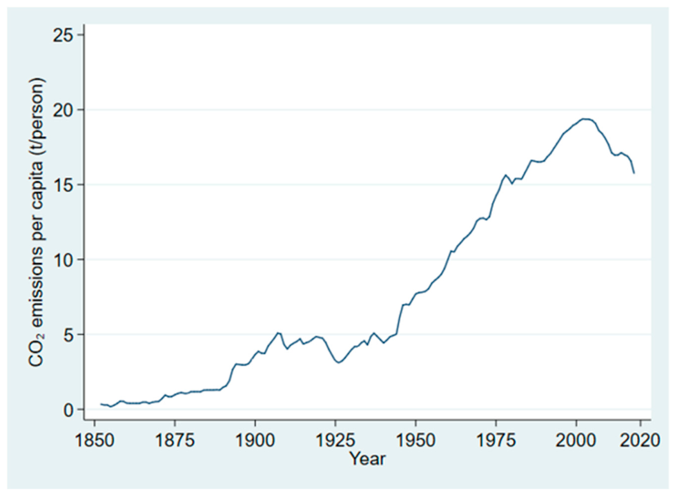
To curb CO₂ emissions, it is necessary to gain a comprehensive and sound understanding of their causes, especially the energy–CO₂ emissions nexus. First, energy efficiency typically refers to the GDP generated per unit of energy consumed [4]. The less energy it takes to create one dollar of GDP, the higher the energy efficiency. Nowadays, the main reason most emerging economies fail to reduce excessive CO₂ emissions is their lack of advanced technology and low energy efficiency [1,10,11]. Figure 1 illustrates the historical trend in CO₂ emissions per capita in Australia between 1850 and 2020.

Figure 1 shows that emissions steadily increased over the period, with growth accelerating significantly after the 1950s. Per capita emissions peaked in the 2000s, at nearly 20 metric tonnes per person. This can be attributed to a period of accelerated industrialization and economic development. After this peak, the trend moved steadily downwards, reflecting declines in per capita emissions and carbon intensity over recent decades. Second, scholars increasingly agree that the use of renewable energy is negatively associated with CO₂ emissions and can significantly improve environmental quality. Meanwhile, it has been demonstrated both theoretically and in practice that promoting renewable energy, such as wind, solar, hydro, biomass, and geothermal energy, relies on sufficient fiscal investment, the expansion of information and communication technology, clean energy application subsidies, and energy infrastructure construction [9,13,14,15]. However, the driving factors for renewable energy development and widespread application are rarely formulated simultaneously in developed countries or emerging economies in the short term [14,16,17].

In addition, the environmental tax has been recognized as an indispensable policy tool that prevents manufacturers, importers, and exporters from emitting greenhouse gases [18,19,20]. Ref. [21] analyzed how carbon taxes achieve significant reductions in CO₂ emissions in Colombia’s energy sector. They argued that the use of economic instruments helps reduce reliance on conventional energy and improve energy efficiency. Moreover, the study by [22] not only provides evidence of the negative effects of environmental tax and renewable energy on CO₂ emissions in 18 Latin American and Caribbean countries, but also reveals that the mitigation effect of renewable energy is considerably higher than that of environmental tax.

In recent decades, most countries have committed to achieving “net zero” emissions and carbon neutrality by proposing ambitious decarbonization plans. Nevertheless, achieving carbon neutrality is a comprehensive, profound systemic change underway across human society, involving all aspects of energy production and use, industrial structure and activities, transportation, agricultural production, urban and rural construction, and residents’ lifestyles. The impact of energy efficiency, environmental regulations, environmentally related taxes, and renewable energy on CO₂ emissions has been widely discussed at a theoretical level [1,23,24,25]. However, the ultimate effect remains inconclusive in the literature, and empirical evidence from Australia on this topic remains scarce.

Empirically, several studies have examined the relationships among energy efficiency, renewable energy, environmentally related taxes, non-renewable energy consumption, and carbon emissions in Australia. For example, studies have examined energy efficiency and carbon emissions [26]; environmental taxes and carbon emissions [27,28,29]; economic growth and energy consumption [8]; renewable and non-renewable energy and carbon emissions [30]. Although these studies have advanced understanding of Australia’s energy transition, gaps remain regarding the relative effectiveness and timing of different climate mitigation policies.

First, the studies primarily focus on a single climate change mitigator or driver of carbon emissions rather than examining multiple climate mitigators in a single study. A unified study is required to assess the relative contributions of each policy variable to climate mitigation. Second, few of these studies examine the short-run and long-run effects, which is critical for policy formulation, since short-run policies may differ from long-run policies. Third, few studies examine bidirectional causation or feedback loops between policy variables and emissions. The aim is to determine whether climate mitigation policies in Australia are proactive or reactive, given Australia’s policy inconsistency in the past, for example, the introduction of the carbon tax in 2012 and its subsequent repeal in 2014.

This paper addresses these gaps by examining the short- and long-run effects of energy efficiency, environmentally related taxes, renewable energy, and non-renewable energy consumption on carbon emissions in Australia within a dynamic ARDL framework. This study extends the current literature in three ways. First, it provides evidence on the relative magnitude of the climate-mitigating effects of the policy variables in the short and long run by comparing their estimated coefficients. Second, it investigates the direction of causality and identifies feedback loops between the variables and carbon emissions using the VECM Granger causality estimator. This offers new insights into whether Australia’s environmental policies are proactive or reactive. Third, the study provides robustness checks that assess the uncertainty surrounding the mixed long-run coefficient estimates using the FMOLS and DOLS estimators. This enabled us to provide policy-relevant information on the relative effectiveness of different climate mitigation variables, their timing, and the uncertainty surrounding these estimates.

While previous studies have confirmed that the use of renewable energy or environmentally related taxes significantly promotes CO₂ emissions mitigation, other scholars have expressed doubts about the effectiveness of these approaches in preventing emissions. For instance, ref. [31] suggested that the low share of renewable energy consumption has not yet reached the critical threshold required to mitigate CO₂ emissions driven by the high energy demands of economic growth in developing countries. In the most recent study, ref. [32] found that international trade is a determinant of increased CO₂ emissions, while trade taxes can help mitigate CO₂ emissions in Belt and Road countries.

As a developed economy, Australia faces the challenge of meeting its CO₂ emissions reduction target while sustaining economic growth and maintaining its prominent role in the global energy production system. Since the 1990s, the local government has implemented several green energy plans to reduce CO₂ emissions and their detrimental effects on the environment. Nevertheless, these plans have not delivered the expected outcomes due to persistent reliance on conventional energy and various challenges associated with the clean energy transition [32]. For instance, ref. [32] revealed that, although climate mitigation plans have been implemented at the government, national, and local levels, Indigenous Australians should form an integral part of climate change adaptation. Furthermore, academic research on Australia’s non-renewable energy consumption and CO₂ emissions remains insufficient. Thus, this paper makes an empirical contribution to the debate about the relationship between CO₂ emissions, energy efficiency, environmentally related taxes, renewable energy, and non-renewable energy consumption in Australia. We believe that exploring the nature of these relationships is important in the context of tackling challenges caused by increasing global warming and weak economic recovery, by assessing the effectiveness of environmentally related taxes, energy efficiency, or increasing renewable energy as the most significant driver(s) of climate mitigation in Australia in the short and long run.

To the best of our knowledge, this paper makes several contributions to the literature on the energy–emissions nexus in Australia. First, this paper examines the short-run and long-run effects of energy efficiency, environmentally related tax, renewable energy, and non-renewable energy consumption within a single empirical framework, whereas previous studies have often examined these factors individually. The findings allow this study to compare the relative magnitude of the effects associated with different climate mitigation variables, providing insights into a dimension that remains underexplored in the Australian context.

Second, the study addresses the timing of these variables’ effects, distinguishing between policy variables with immediate effects and those that take longer to manifest. Third, the study examines the direction of causality using VECM-based Granger causality tests and assesses the robustness of the estimated long-run relationships with FMOLS and DOLS estimators. Collectively, these contributions provide a more nuanced and policy-relevant understanding of Australia’s energy–emissions nexus than previous studies.

The remaining sections of this paper are organized as follows: Section 2 provides an overview of Australian energy sources and CO₂ emissions. Section 3 reviews the literature. Section 4 presents the data and research methods. Section 5 reports, analyzes, and discusses the findings, and Section 6 presents the conclusion and policy recommendations.

2. Overview of Australia’s Energy Sources and CO₂ Emissions

A major challenge in energy efficiency is the “rebound effect,” the phenomenon in which improvements in energy efficiency lead to increased energy consumption due to behavior changes or other factors. For example, if a consumer replaces an old, inefficient appliance with a more efficient one, they may be more likely to use it more frequently or for longer periods, offsetting some of the energy savings. The rebound effect is an important consideration when designing and implementing energy efficiency policies, as it can limit the effectiveness of such measures. Over the past three decades, total CO₂ emissions across all energy sources in Australia have increased from approximately 250 million tons to 387 million tons, and the energy source structure of CO₂ emissions has also undergone significant changes. Significant changes and challenges are also emerging in the transportation and industrial sectors as efforts to mitigate climate change and ensure energy security progress. The Australian energy sector is undergoing a rapid transformation, driven by changes in consumer behavior and systemic decarbonization efforts.

2.1. Carbon Emissions by Energy Source in Australia

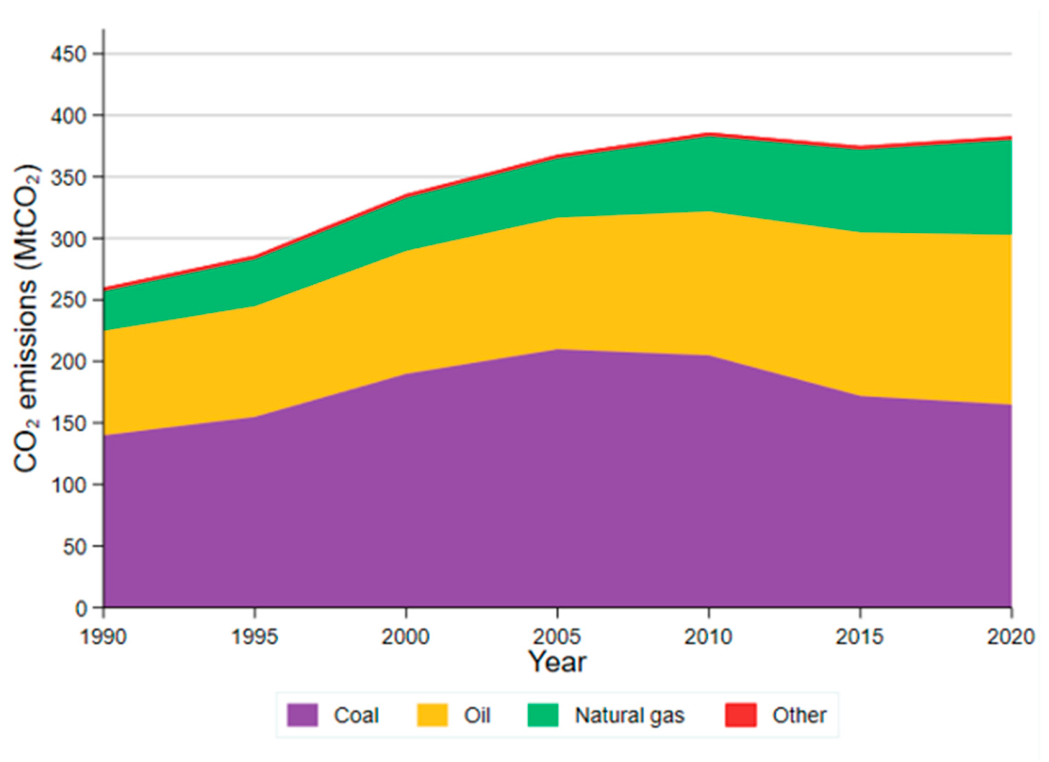
Figure 2 shows the dynamic changes in CO₂ emissions by energy source. CO₂ emissions from coal and oil account for 70.45% of total emissions and follow the same trend, namely “first increase before 2010 and then decrease in the following ten years”. CO₂ emissions from natural gas consumption have nearly doubled over the past 30 years, indicating significant expansion in natural gas use. Australia is rich in oil and gas resources, with 21 basins (or structural units) where oil and gas have been discovered. The proven reserves of conventional crude oil in Australia are 17.57 × 10⁸ t, the proven reserves of conventional natural gas are 7.06 × 10¹² m³ (56.65 × 10⁸ t oil equivalent), and the proven reserves of shale gas are 0.06 × 10¹² m³ (0.55 × 10⁸ t oil equivalent).

Proven natural gas reserves account for 78% of the country’s total proven oil and gas reserves, and sea-area natural gas reserves account for 82% of the country’s total proven natural gas reserves. By the end of 2012, seven liquefied natural gas (LNG) projects were under construction in Australia, with 14 production lines and a total designed annual production capacity of 6180 × 10⁴ t. However, electricity generation from natural gas on Australia’s main grid fell 23% in 2020 to its lowest level in a decade, while large-scale wind, solar, and rooftop solar PV installations continued to increase. The Australian Energy Market Operator (AEMO) noted in its Annual Gas Statement of Opportunities report that total Australian gas consumption is likely to decline over the next 20 years and may disappear from the grid due to very weak competitiveness relative to renewable energy or green hydrogen.

2.2. Carbon Emissions by Sector in Australia

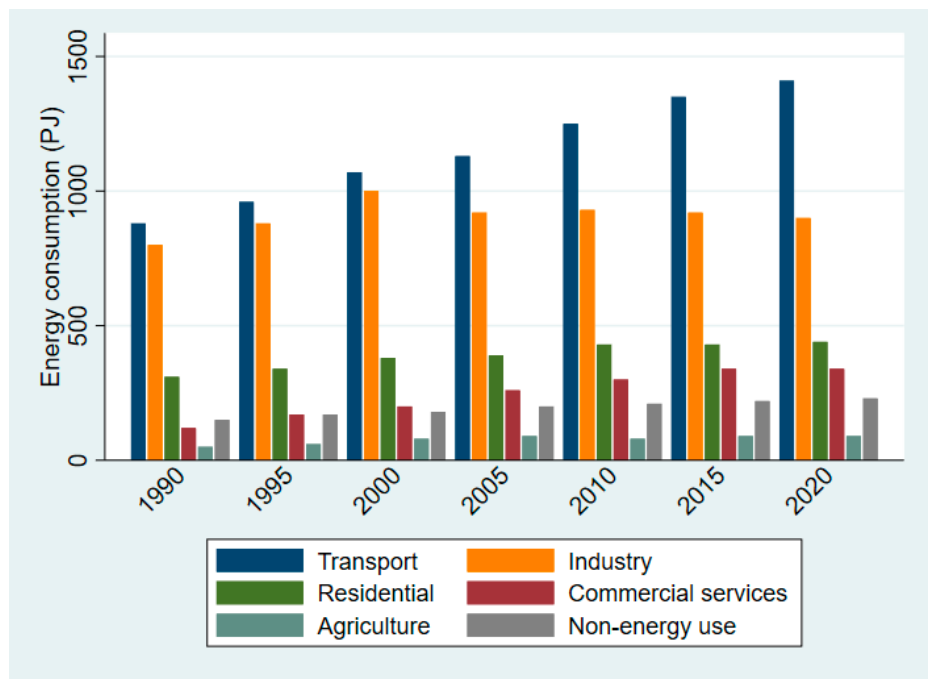
The transportation and industry sectors are the two major contributors to energy consumption, accounting for 65.9% of total primary energy consumption across all sectors. In other words, these sectors suffer from energy over-consumption and CO₂ over-emissions, resulting in increasing pressure to improve energy efficiency [34]. Commercial, public service, and residential energy consumption also grew rapidly, with increases of 111.11% and 43.33%, respectively, as the economy developed. The agriculture and forestry sector consumed the least energy, accounting for only 6.02% of total national energy consumption, as illustrated in Figure 3. Among them, the energy consumption caused by the transportation sector quickly increased from around 900 petajoules (PJ) to 1400 PJ, increasing by 35.71% from 1990 to 2020, while the energy consumption from the industry sector first increased from 800 PJ to 1000 PJ during 1990–2000 and then decreased to around 900 PJ in 2020. In the energy consumption sector, transport and industry are the two priority sectors with the potential to reduce energy demand and CO₂ emissions.

The overview above shows that Australia’s energy system is largely driven by non-renewable energy sources, thereby increasing carbon emissions, which are dominated by fossil fuel combustion. Understanding the Australian energy system guides policy formulation on energy efficiency and informs relevant empirical studies. To address the energy efficiency gap, a range of policy instruments and strategies has been proposed, including energy efficiency standards and labels, subsidies and incentives for energy-efficient technologies and practices, and education and awareness-raising campaigns. These policies aim to correct market failures, reduce information asymmetry, and overcome behavioral barriers. Overall, the contextual overview of energy efficiency involves understanding the factors that contribute to the energy efficiency gap, identifying policy instruments and strategies to address it, and considering potential rebound effects.

3. Literature Review

There is a vast body of literature on the nexus among energy efficiency, environmental taxes, renewable energy, and CO₂ emissions. However, the literature has not reached consensus on these associations. The study summarizes the current literature across three main groups linking CO₂ emissions to energy efficiency, environmentally related taxes, and renewable energy.

3.1. The Impact of Energy Efficiency and CO₂ Emissions

Scholars in the natural sciences have developed numerous approaches to improve energy efficiency and reduce CO₂ emissions. Ref. [35] proposed a cleaner powertrain solution for a 240-ton heavy-duty mining haul truck using an integrated design-and-control optimization method. The study found that the truck’s energy efficiency increased and that carbon dioxide emissions decreased by 21%. Ref. [36] presented an optimized solution for dimethyl carbonate production by combining heat integration routes with reactive and pressure-sensitive distillation columns, resulting in 38.33% energy savings and a 37.5% reduction in CO₂ emissions. In addition, energy efficiency in buildings [37,38], the metal sector [39], port container terminal equipment [40], and the water supply system [38] were explored. The impact on CO₂ emissions was analyzed under various scenarios.

By contrast, studies in the social sciences often examine the relationship between energy efficiency and CO₂ emissions using various econometric approaches. For instance, ref. [41] explored the impact of energy efficiency on CO₂ emissions using panel data from 30 developing countries from 1990 to 2016. They found that energy efficiency played a key role in reducing energy intensity and mitigating CO₂ emissions. Ref. [42] tested energy efficiency in China and Nigeria. The authors found that improvements in energy efficiency increase CO₂ emissions in China, while CO₂ emissions declined in Nigeria, where industrial energy consumption remains low. Based on data from 30 OECD countries, ref. [26] investigated the impact of energy efficiency improvements on CO₂ emissions by decomposing energy efficiency into economic factors (structural shifts) and non-economic factors (consumer lifestyles), and found that, overall, improving energy efficiency reduced CO₂ emissions.

In a related study, ref. [1] examined the mitigating role of energy efficiency, renewable energy, environmental technology, and economic growth in improving environmental quality across 16 OECD high-income countries. The study found that energy efficiency, renewable energy, and technology reduce carbon emissions, with energy efficiency having the strongest effect. In contrast, non-economic behavioral factors have a non-trivial influence on CO₂ emissions. The study by [43] provided evidence that lower integrated efficiency of inputs and outputs, and of energy, in China’s agricultural sector resulted in higher CO₂ emissions intensity.

Ref. [44] examined the direct and total carbon footprint of the Australian utility service sector from 2013 to 2017 using an input–output framework and the Australian Industrial Ecology Virtual Laboratory platform. The findings indicate that the service sector accounts for 37.2% of direct carbon emissions and 43.1% of the total carbon footprint, with manufacturing and commercial services responsible for the largest indirect emissions. Additional tests on the service subsectors (electricity generation, transmission and distribution of electricity, gas and water supply, and waste collection and treatment) reveal that electricity generation and transmission are the most significant subsectors for maximizing the use of low-carbon technologies.

3.2. The Link Between Environmentally Related Taxes and CO₂ Emissions

The aim of implementing environmentally related taxes is to reduce energy intensity and improve economic efficiency [45]. Over the past three decades, most nations worldwide, including Australia, have imposed environmentally related taxes to varying degrees to reduce CO₂ emissions [46]. Energy taxes account for approximately 2% of GDP and 5% of tax revenues in those European countries [15]. The study of [47] revealed that implementing environmentally related taxes promotes energy efficiency by encouraging enterprises and policymakers to develop environmental technology innovation. The findings of [48] also indicated that environmental taxes help control carbon emissions and their harmful environmental impacts.

Ref. [49] investigated China’s diesel tax policy and found that a diesel tax adjustment led to a 0.096% reduction in annual carbon emissions. Ref. [50] emphasized that sectors differ in their energy structures and CO₂ emission intensities, and that differentiated environmental tax rates at the sectoral level should be designed. The study also found that the optimized energy-related taxation scheme promotes the transformation of China’s energy structure and reduces CO₂ emissions. Ref. [51] employed the Bootstrapped Quantile Regression and Method-of-Moments Quantile Regression estimators. The study examined the moderating role of governance quality in promoting environmental regulation, environmental taxes, and technology in the energy transition in OECD countries. The results show that governance quality improves the effectiveness of environmental regulation, environmental taxes, and technology in the energy transition process. Moreover, environmental taxes are more robust in the 20th and 40th quantiles of the energy transition, while the effect declines at the upper quantiles.

However, some studies have also observed and analyzed negative effects of environmental taxes on revenue and economic growth. For instance, ref. [52] examined the impact of financial development on energy intensity, with taxes as a mediator, and found that the energy intensity of developing countries tends to decline under financial and tax reform, thereby increasing CO₂ emissions. Based on observations of heterogeneous companies, ref. [53] argued that environmental taxation had a positive effect on state-owned companies, stimulating them to increase environmental investment. Still, it increased the operating costs of small and medium-sized companies. Their contribution to CO₂ emissions reduction is weak. In 38 OECD countries, ref. [28] found that environmental taxation reduces CO₂ emissions in moderate- and high-emission countries but is ineffective in countries with already low emissions. The study further noted that environmental taxes have reduced coal and oil consumption in favor of natural gas consumption.

3.3. The Influence of Renewable Energy Consumption (RE) on CO₂ Emissions

It is widely accepted that renewable energy is a key determinant of CO₂ emissions mitigation [14,54]. Transitioning to a renewable-energy-oriented energy structure is widely regarded as the backbone of global energy policy and an effective path to decoupling economic growth from fossil fuel consumption [55,56]. The rapid expansion of renewable energy sources can be attributed to the rapid decline in generation costs and the adoption of low-carbon technologies over the last three decades [9].

The study by [57] examined the relationship among energy-related CO₂ emissions, economic growth, and RE in the U.S. from 1997 to 2017. The study confirmed that RE, electricity prices, and primary energy prices increase emissions. Refs. [58,59] confirmed that renewable energy and export quality reduce CO₂ emissions despite positive economic growth in advanced countries. Ref. [60] also revealed, based on an analysis of Thailand, that RE has a negative and statistically significant impact on CO₂ emissions in the short run.

By applying innovative multivariate wavelet analysis tools, ref. [61] investigated associations among renewable and non-renewable energy consumption, GDP, and CO₂ emissions in Vietnam and found that the interlinkages among these variables are time-varying over the 1985–2019 period. The findings indicate that an increase in renewable energy consumption does not necessarily reduce CO₂ emissions. This outcome depends on the national development phase and overall energy demand. Similarly, ref. [62] examine the nonlinear effects of RE and economic growth on CO₂ emissions using a dynamic panel threshold model and concluded that increased RE reduces CO₂ emissions only if the country exceeds a certain RE threshold. Ref. [30] used panel ARDL to examine the short- and long-run effects of renewable and nonrenewable energy on carbon emissions in eight of the most polluted developing and developed countries (Argentina, South Africa, Iran, Brazil, Morocco, Canada, Poland, and Germany) and found that renewable energy reduces carbon emissions while nonrenewable energy heightens environmental degradation.

4. Data and Method

4.1. Data Source

This section provides a comprehensive description of the data and its sources. CO₂ represents carbon emissions (metric tons per capita) (Series code: EN.ATM.CO2E.PC); EE is the energy intensity level of primary energy (Series code: EG.EGY.PRIM.PP.KD); EC describes non-renewable energy consumption (% of total energy consumption) (Series code: EG.USE.COMM.FO.ZS); ERT represents environmentally related tax (% of GDP); and RE represents renewable energy consumption (% of total final energy consumption) (Series code: EG.FEC.RNEW.ZS). The time series data for CO₂, EE, EC, and RE were obtained from the World Bank World Development Indicators (WDI) Database [63] covering the period between 1990 and 2020. ERT time series were obtained from the OECD environment database. Furthermore, the data, including their descriptions, units, and symbols (abbreviations), are presented in

Table 1. Variable Description, Symbol, and Source.

Variables	Description	Symbol	Source
Carbon emissions	CO2 emissions (metric tons per capita)	CO2	WDI
Energy efficiency	Energy intensity level of primary energy (Megajoules/$2021 PPP GDP)	EE	WDI
Energy consumption	Energy consumption from non-renewable sources (% of total energy consumption)	EC	WDI
Environmentally related tax revenue	Environmental tax (% of GDP)	ERT	OECD
Renewable energy	Renewable energy consumption (% of total final energy consumption)	RE	WDI

. In addition, the graphical illustration of the variables studied is presented in Figure 4. To obtain the empirical results, this study used EViews 14.

4.2. Model Specification

$${LCO}_{2t}={f(\mathrm{L}EE}_t,{LEC}_t,{LERT}_t,{LRE}_t)$$

(1)

In Equation (1), CO₂ denotes the log of carbon emissions, EE denotes the log of energy efficiency, EC denotes the log of non-renewable energy consumption, ERT denotes the log of environmentally related tax, and RE denotes the log of renewable energy consumption. The data used in this paper were first transformed to logarithmic form to address concerns about heteroscedasticity and large coefficients.

4.3. Econometric Strategy

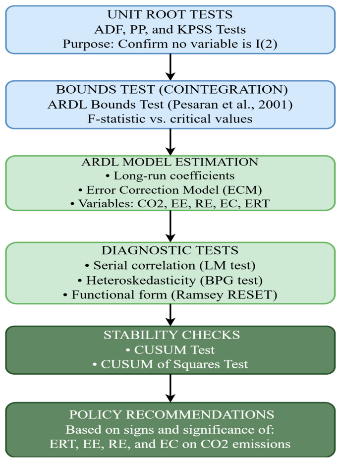
The comprehensive econometric strategy of the present study is shown in Figure 4. The study selected CO₂ emissions as the dependent variable, while energy efficiency (LEE), environmentally related tax (LERT), renewable energy (LRE), and non-renewable energy consumption (LEC) were independent variables over the period 1990 to 2020. The study’s analysis includes a unit root test, a Zivot–Andrews structural break unit root test, a linear bounds test, a Granger causality test, and an ARDL model. In addition, we run Fully Modified Ordinary Least Squares (FMOLS) and Dynamic Ordinary Least Squares (DOLS) for robustness checks. Finally, we present the study’s conclusion, policy recommendations, and limitations.

4.4. Unit Root Tests

To assess the stationarity of the selected dependent and independent variables, the authors conducted unit root tests using the ADF [65], PP [66], and KPSS [67]. Unit root tests are statistical tests used in time series analysis to determine whether a time series is stationary or non-stationary. Stationarity is an important concept in time series analysis because many statistical methods and models assume that the data are stationary, meaning their statistical properties do not change over time. Unit root tests help researchers and analysts assess the stationarity of a time series. A non-stationary time series has statistical properties, such as the mean and variance, that change over time, making it challenging to apply standard time series models and techniques effectively and leading to spurious regression. Consistent with the ARDL conditions, all variables should be stationary at their levels or in first differences. Accordingly, the variables were examined before applying the ARDL bounds cointegration test [65,68].

The unit root test equations are provided in Equations (2)–(4) below.

Augmented Dickey–Fuller (ADF)

$${∆\mathrm{Y}}_{\mathrm{t}}=\alpha +\beta t+\gamma Y_{t-1}+{\displaystyle \sum _{i=1}^p}{\delta }_i∆Y_{t-1}+{\epsilon }_t$$

(2)

where $∆$ is the difference operator; ${\mathrm{Y}}_{\mathrm{t}}$ represents the variable of interest; $p$ is the lag length, and ${\epsilon }_t$ denotes the white noise error term. The null hypothesis tests whether the time series has a unit root.

Phillips–Perron (PP)

$${∆\mathrm{Y}}_{\mathrm{t}}=\alpha +\beta t+\gamma Y_{t-1}+{\epsilon }_t$$

(3)

Kwiatkowski Phillips Schmidt Shin (KPSS)Test

$${∆\mathrm{Y}}_{\mathrm{t}}=\alpha +\beta t+r_t+{\epsilon }_t$$

(4)

where $\beta t$ is the deterministic time trend; $r_t$ represents the random walk ($r_t=r_{t-1}+u_t$); $u_t~u_{t }i.i.d (0,{\sigma }_u^2)$. ${\epsilon }_t$ is a stationary error term. The null hypothesis is that the data is stationary.

4.5. Estimation Technique

The study employed the dynamic ARDL technique as the primary estimator. The model introduced by [64,69] includes the lagged values of both the dependent and independent variables on the right-hand side of the equation to capture the dynamic (time-dependent) relationships. This specification allows the model to capture the short- and long-run effects of the independent variables on the dependent variable, making it valuable for empirical research and policy analysis [70]. ARDL can be applied to time series that are integrated of order zero I(0), order one I(1), or a mixture of order zero I(0) and order one I(1). Ref. [28] show that the ARDL model can assess many potentially coherent hypotheses and theories when the dependent variable is examined at level I(0) or after taking the first difference I(1).

The model is suitable for studies with small sample sizes [71,72]. Given this study’s small sample size (31), the ARDL technique is appropriate for estimating relationships among the variables. Researchers often use this model to gain insights into the interplay among economic variables over time [73,74]. Additionally, the ARDL model is widely used across fields, including environmental economics, finance, and the social sciences, to analyze long-run relationships among economic and environmental variables [28,30,71,75,76].

4.5.1. ARDL Bounds Cointegration Test

To examine any long-run relationship among the variables studied, cointegration must be established. Cointegration is a valuable statistical property that indicates whether two time series move together in the long run. In economics and finance, cointegration improves forecasting and helps separate short-run dynamics from long-run equilibrium [73,74]. To establish the presence of a long-run association among CO₂ emissions, EE, ERT, EC, and RE, the current study employs the ARDL bounds cointegration test by [58]. The ARDL bounds co-integration test is confirmed by the equation below:

$$\begin{array}{c}∆{\mathrm{L}\mathrm{C}\mathrm{O}}_{2\mathrm{t}}\hfill \\ ={\mathrm{\alpha }}_0+{\displaystyle \sum _{\mathrm{i}=1}^{\mathrm{r}}}{\mathrm{\sigma }}_{1\mathrm{i}}∆\mathrm{L}{\mathrm{C}\mathrm{O}}_{2\mathrm{t}-\mathrm{i}}+{\displaystyle \sum _{\mathrm{i}=0}^{\mathrm{r}}}{\mathrm{\sigma }}_{2\mathrm{i}}{∆\mathrm{L}\mathrm{E}\mathrm{E}}_{\mathrm{t}-\mathrm{i}}+{\displaystyle \sum _{\mathrm{i}=0}^{\mathrm{r}}}{\mathrm{\sigma }}_{3\mathrm{i}}{∆\mathrm{L}\mathrm{E}\mathrm{R}\mathrm{T}}_{\mathrm{t}-\mathrm{i}}+{\displaystyle \sum _{\mathrm{i}=0}^{\mathrm{r}}}{\mathrm{\sigma }}_{4\mathrm{i}}{∆\mathrm{L}\mathrm{R}\mathrm{E}}_{\mathrm{t}-\mathrm{i}}\hfill \\ +{\displaystyle \sum _{\mathrm{i}=0}^{\mathrm{p}}}{\mathrm{\sigma }}_{5\mathrm{i}}∆\mathrm{L}{\mathrm{E}\mathrm{C}}_{\mathrm{t}-1}+{\mathrm{\lambda }}_1{\mathrm{L}\mathrm{C}\mathrm{O}}_{2\mathrm{t}-1}+{\mathrm{\lambda }}_2\mathrm{L}{\mathrm{E}\mathrm{E}}_{\mathrm{t}-1}+{\mathrm{\lambda }}_3\mathrm{L}{\mathrm{E}\mathrm{R}\mathrm{T}}_{\mathrm{t}-1}+{\mathrm{\lambda }}_4{\mathrm{L}\mathrm{R}\mathrm{E}}_{\mathrm{t}-1}+{\mathrm{\lambda }}_5{\mathrm{L}\mathrm{E}\mathrm{C}}_{\mathrm{t}-1}\hfill \\ +{\mathrm{\epsilon }}_{\mathrm{t}}\hfill \end{array}$$

(5)

where $∆$ denotes the first difference operator, ${\sigma }_1$ to ${\sigma }_5$ represents the short-run coefficients of the explanatory variables. ${\lambda }_1$ to ${\lambda }_5$ represents the coefficients of the lagged level variables used to compute the long-run multipliers. The lag lengths $r$ and $p$ are selected using the Akaike information criterion. CO₂ is carbon dioxide emissions, EE is energy efficiency, ERT represents an environmentally related tax, RE denotes renewable energy consumption, and EC is non-renewable energy consumption. ${\mathrm{\epsilon }}_{\mathrm{t}}$ is the white noise error term.

The null hypothesis of no cointegration states that in the long run, the coefficients of the variables are equal to zero, i.e., ${\mathrm{H}}_0:$ ${\lambda }_1$ = ${\mathrm{\lambda }}_2$ = ${\mathrm{\lambda }}_3$ = ${\mathrm{\lambda }}_4$ = ${\mathrm{\lambda }}_5=$ 0. This is tested against the joint alternative that the level coefficients of the variables are not all zero, i.e., ${\mathrm{H}}_1:$ ${\mathrm{\lambda }}_1{\ne \mathrm{\lambda }}_2{\ne \mathrm{\lambda }}_3{\ne \mathrm{\lambda }}_4{\ne \mathrm{\lambda }}_5\ne$ 0.

Co-integration is inferred from the relationship between the F-statistic and the lower and upper critical bounds. The lower critical bound assumes all series are I(0), and the upper critical bound assumes all series are I(1). The series are cointegrated if the F-statistic exceeds the upper critical bound. Conversely, no cointegration is confirmed if the F-statistic falls below the lower critical bound. Cointegration is inconclusive if the F-statistic is between the lower and upper critical bounds.

4.5.2. Lag Selection

The study conducted preliminary lag-order selection to determine the optimal lag length for the ARDL estimation using information criteria. The study set the maximum lag length to 4 and applied the final prediction error (FPE), Akaike information criterion (AIC), Hannan–Quinn information criterion (HQIC), and Schwarz Bayesian Information Criterion (SBIC). FPE, AIC, and HQIC all selected lag 2, while SBIC selected lag 1. The study prioritized lag 2, as indicated by FPE, AIC, and HQIC, and re-estimated the model for robustness with a maximum lag length of 4. The selected ARDL lag order is 2 1 1 1 1, indicating 2 lags for the dependent variable and 1 lag for each independent variable.

In the presence of cointegration, the dynamic ARDL-ECM is estimated to capture the short-run dynamics and the long-run equilibrium adjustment. Short-run dynamics are derived from the coefficients on the differenced lagged variables, while long-run adjustment is indicated by the coefficient on the error correction term (${\mathrm{E}\mathrm{C}\mathrm{T}}_{\mathrm{t}-1}$). The ARDL-ECM model is specified in the equation below and estimated with the optimal lag order ARDL (2 1 1 1 1).

$$\begin{array}{c}∆\mathrm{L}{\mathrm{C}\mathrm{O}}_{2\mathrm{t}}={\mathrm{\alpha }}_0+{\displaystyle \sum _{\mathrm{i}=1}^2}{\mathrm{\beta }}_{1\mathrm{i}}{∆\mathrm{L}\mathrm{C}\mathrm{O}}_{2\mathrm{t}-\mathrm{i}}+{\displaystyle \sum _{\mathrm{i}=0}^1}{\mathrm{\beta }}_{2\mathrm{i}}{∆\mathrm{L}\mathrm{E}\mathrm{E}}_{\mathrm{t}-\mathrm{i}}+{\displaystyle \sum _{\mathrm{i}=0}^1}{\mathrm{\beta }}_{3\mathrm{i}}{∆\mathrm{L}\mathrm{E}\mathrm{R}\mathrm{T}}_{\mathrm{t}-\mathrm{i}}\hfill \\ \hspace{1em}\hspace{1em}\hspace{1em}\hspace{1em}\hspace{1em}\hspace{1em}+{\displaystyle \sum _{\mathrm{i}=0}^1}{\mathrm{\beta }}_{4\mathrm{i}}{∆\mathrm{L}\mathrm{R}\mathrm{E}}_{\mathrm{t}-\mathrm{i}}+{\displaystyle \sum _{\mathrm{i}=0}^1}{\mathrm{\beta }}_{5\mathrm{i}}∆\mathrm{L}{\mathrm{E}\mathrm{C}}_{\mathrm{t}-\mathrm{i}}+\mathrm{\phi }·{\mathrm{E}\mathrm{C}\mathrm{T}}_{\mathrm{t}-1}\hfill \\ \hspace{1em}\hspace{1em}\hspace{1em}\hspace{1em}\hspace{1em}\hspace{1em}+{\mathrm{u}}_{\mathrm{t}}\hfill \end{array}$$

(6)

From Equation (6), the short-run dynamics are derived from the β coefficients of the first-differenced variables. ${\mathrm{E}\mathrm{C}\mathrm{T}}_{\mathrm{t}-1}$ represents the lagged residuals from the long-run cointegration equation. For cointegration to be confirmed, the ECT must be negative and significant, with a value between −1 and 0. $\phi$ is the rate of adjustment that restores long-run equilibrium after a short-run deviation. ${\mathrm{u}}_{\mathrm{t}}$ is the disturbance term.

The estimation was performed using an unrestricted intercept with no deterministic trend. The effective sample size is 28 observations taking into account lags and differencing. The final model has 8 parameters estimated, which corresponds to approximately 3.5 observations per parameter.

Although the ARDL bounds testing approach is widely used to establish long-run relationships, it assumes that the regressors are weakly exogenous. This assumption leaves the ARDL model vulnerable to endogeneity. For instance, simultaneity may occur when two variables in the model influence each other at the same time (contemporaneously); a very important determinant of carbon emissions may be omitted from the model (omitted variable, e.g., technology); and reverse causality may arise, where the dependent variable influences the independent variable rather than the other way around. Although ARDL attempts to mitigate endogeneity by using lags of the dependent and independent variables, this only partially addresses the issue. To address these potential endogeneity problems and examine the direction of causality, the study augments the ARDL framework with VECM-based Granger causality tests. The VECM provides F-statistics for short-run causality and t-statistics on the lagged error correction term (ECT) for long-run causality.

To assess the robustness of the ARDL long-run results, the study also employs Fully Modified OLS (FMOLS) and Dynamic OLS (DOLS) estimators. FMOLS and DOLS are designed to correct for potential endogeneity and serial correlation in cointegrating regressions. FMOLS introduces a nonparametric adjustment, whereas DOLS addresses endogeneity parametrically by including leads and lags of the differenced regressors. These estimators are applied only to the long-run coefficients and serve as a robustness check for the ARDL long-run results.

4.5.3. Granger Causality Tests

The bounds cointegration test confirms the presence of a long-run relationship among variables, implying that they move together over time. However, it does not reveal the direction of causation between the dependent and independent variables. To identify short- and long-run causal relationships among CO₂ emissions, energy efficiency (EE), environmentally related tax (ERT), renewable energy (RE) sources, and non-renewable energy consumption (EC), the study employs the VECM Granger causality test, which distinguishes between short- and long-run relationships [77]. Short-run causality is examined through the joint significance of the lagged differenced variables, while long-run causality is assessed through the significance of the error correction term. Granger causality has been widely used across various fields, including economics, finance, and neuroscience, to analyze time series data and explore potential causal relationships between variables.

Following [71] the study employed an expanded version of the Granger-causality approach expressed as a multivariate ρth-order VECM below:

$$\begin{array}{c}{∆\mathrm{L}\mathrm{C}\mathrm{O}}_{2t}\hfill \\ ={\alpha }_1+{\displaystyle \sum _{i=1}^p}{\phi }_{11i}{∆\mathrm{L}\mathrm{C}\mathrm{O}}_{2t-1}+{\displaystyle \sum _{i=1}^p}{\phi }_{12i}{∆\mathrm{L}\mathrm{E}\mathrm{E}}_{t-1}+{\displaystyle \sum _{i=1}^p}{\phi }_{13i}{∆\mathrm{L}\mathrm{E}\mathrm{R}\mathrm{T}}_{t-i}+{\displaystyle \sum _{i=1}^p}{\phi }_{14i}{∆\mathrm{L}\mathrm{R}\mathrm{E}}_{t-1}\hfill \\ +{\displaystyle \sum _{i=1}^p}{\phi }_{15i}{∆\mathrm{L}\mathrm{E}\mathrm{C}}_{t-1}+{\lambda }_1{\mathrm{E}\mathrm{C}\mathrm{T}}_{t-1}\hfill \\ +{\mu }_{1t}\hfill \end{array}$$

(7)

where $∆$ is the first-difference operator; ${\mathrm{L}\mathrm{C}\mathrm{O}}_{2\mathrm{t}}$ represents carbon emissions at time, $\mathrm{t}$; ${\alpha }_1$ is the constant; $p$ is the number of selected lags using the information criterion; Energy efficiency (LEE), environmentally related tax (LERT), renewable energy (LRE), and non-renewable energy consumption (LEC) are the individual independent variables; ${\phi }_1$–${\phi }_5$ denote the short-run coefficients of the lagged differenced variables; ${\lambda }_1$ is the coefficient of the error correction term, which captures evidence of long-run causality; ${\mathrm{E}\mathrm{C}\mathrm{T}}_{\mathrm{t}-1}$ represents the lagged residual from the long-run cointegration equation; ${\mu }_{1t}$ is the white noise error term.

5. Results and Discussion

Summary statistics are presented in

Table 2. Summary statistics.

Variables	Obs.	Mean	Median	Maximum	Minimum	Std. Dev.	Skewness	Kurtosis
CO2	31	1.223	1.22	1.267	1.182	0.029	0.003	1.387
EE	31	4.707	6.64	6.01	3.444	0.684	−0.037	2.015
ERT	31	1.022	1.029	1.205	0.739	0.118	−0.511	2.667
RE	31	8.357	8.37	10.13	6.68	0.994	−0.201	2.106
EC	31	1.954	1.956	1.966	1.929	0.008	−1.11	3.874

. The mean CO₂ emission is 1.22, with a standard deviation of 0.02. Energy efficiency has a mean of 4.71 and a standard deviation of 0.68. The mean environmentally related tax is 1.02, with a standard deviation of 0.11. The mean value of renewable energy is 8.35, with a standard deviation of 0.99. Lastly, non-renewable energy consumption has a mean of 1.95, with a standard deviation of 0.008. The skewness and kurtosis values indicate that the variables are approximately symmetric. The total number of observations in this study is 31.

Moreover, the correlation matrix in

Table 3. Correlation matrix.

Variables	LCO2	LEE	LERT	LRE	LEC
LCO2	1.000
LEE	−0.443 **	1.000
	(−2.664)	-----
LERT	−0.400 ***	0.002	1.000
	(−5.281)	(0.011)	-----
LRE	−0.569 ***	0.579 ***	−0.381 **	1.000
	(−4.857)	(3.828)	(−2.221)	-----
LEC	0.574 ***	−0.408 ***	0.548 ***	−0.589 ***	1.000
	(4.917)	(−5.410)	(3.535)	(−3.928)	-----

Note: ** and *** indicate statistical significance at the 5% and 1% levels, respectively.

shows a positive correlation between CO₂ emissions and non-renewable energy consumption (EC), indicating that non-renewable energy sources increase CO₂ emissions in Australia. In contrast, negative and significant correlations were found among CO₂ emissions, energy efficiency, environmentally related taxes, and renewable energy sources, indicating that higher energy efficiency, environmentally related taxes, and consumption of renewable energy play a crucial role in reducing CO₂ emissions.

Table 4. Unit root test results.

	ADF		PP		KPSS
Variable	Level	1st Difference	Level	1st Difference	Level	1st Difference
LCO2	0.020	−3.456 ***	−0.004	−3.536 ***	0.186	0.388 ***
LEE	2.311	−4.108 ***	4.653	−4.528 ***	0.717	0.057 ***
LERT	0.882	−4.692 ***	0.812	−4.665 ***	0.411	0.472 **
LEC	−0.379	−4.509 ***	−0.332	−4.576 ***	0.170	0.367 **
LRE	−0.510	−5.806 ***	−0.592	−5.792 ***	0.234	0.180 ***

Note: ** and *** indicate statistical significance at the 5% and 1% levels, respectively.

presents the results of the unit root tests. The results indicate that all variables are stationary only after first differencing (I(1)). Since none of the variables is integrated of order 2, the ARDL bounds testing approach is appropriate for examining the presence of a long-run relationship among the variables.

Additionally, the study used the [78] test to account for unknown structural breaks in the time series. The ZA test goes beyond traditional unit root tests by allowing for structural breaks, providing researchers and analysts with more reliable insights into the stationarity properties of time series data and enhancing the quality of modeling and forecasting efforts. The ZA test detects the most significant endogenous structural break for each variable over the sampled period rather than accounting for all potential structural breaks within each time period. It identifies not only whether a unit root exists but also when and how the structural breaks occurred. The identified structural break is then explained by linking it to a known Australian policy shift during that period.

The test provides decision criteria for determining whether a time series is stationary (free of unit roots) or exhibits unit roots with structural breaks. This information is crucial for selecting appropriate time series models and making accurate forecasts. The outcomes of the ZA structural unit-root tests with a single break year are presented in

Table 5. Zivot and Andrews’ structural break unit root test.

	Variables	Level	BDS	1st Difference	BDS	Integration
	LCO2	−2.636	2018	−4.976 ***	2007	1(1)
	LEE	−1.909 ***	2010	−7.353 ***	2018	1(1)
intercept	LERT	−5.026 ***	1999	−6.778 ***	2004	1(0)
	LEC	−3.344	2017	−5.634 ***	2014	1(1)
	LRE	−3.945	2017	−6.554 ***	2010	1(1)
	LCO2	−2.646	2009	−5.073 **	2008	1(1)
	LEE	−5.416 ***	2017	−7.552 ***	2018	1(1)
Trend & Intercept	LEC	−4.101	2015	−5.594 ***	2013	1(1)
	LERT	−4.796 **	1999	−6.434 ***	2004	1(0)
	LRE	−4.067	2002	−6.660 ***	2008	1(1)
	LCO2	−5.247 ***	2008	−4.969 **	2015	1(0)
	LEE	−5.088 ***	2015	−7.176 ***	2017	1(0)
Trend	LEC	−4.615 **	2015	−5.266 ***	2004	1(1)
	LERT	−4.967 **	2001	−5.668 ***	1995	1(0)
	LRE	−3.139	2007	−6.042 ***	2004	1(1)

Note: ** and *** indicate statistical significance at the 5%, and 1% levels, respectively.

. At the intercept level, the structural break years were 2018 for CO₂ emissions, 2010 for LEE, 1999 for LERT, 2017 for LEC, and 2017 for LRE. At the trend and intercept level, the structural break years were 2009 for LCO₂ emissions, 2017 for LEE, 2013 for LERT, 1999 for LEC, and 2002 for LRE. At the trend level, the structural break years were 2008 for LEE, 2015 for LERT and LEC, 2001 for LRE, and 2007 for LRE.

These structural breaks correspond to significant shifts in Australia’s climate and energy policy. The 1999–2000 breakpoints coincide with the introduction of the mandatory renewable energy target [79]. The 2007–2008 breakpoints align with Australia’s ratification of the Kyoto Protocol, a national commitment to reduce greenhouse gas emissions [80]. The 2014 breakpoint coincides with the repeal of the carbon tax [27]. The 2017–2018 breakpoints coincide with discussions of the National Energy Guarantee amid rising energy prices.

Table 6. Lag Selection Criterion.

Lag	LL	LR	FPE	AIC	HQIC	SBIC
0	−297.841		103,000	20.056	20.1009	20.1962
1	−265.729	64.223	22,168.5	18.5153	18.6946	19.0757 *
2	−253.005	25.449 *	17,669.8 *	18.267 *	18.5807 *	19.2478
3	−246.11	13.789	21,443	18.4073	18.8556	19.8085
4	−240.506	11.208	29,853.8	18.6337	19.2165	20.4553

Note: * indicates the optimal lag order selected by the corresponding information criterion.

presents the lag selection criteria for the log-likelihood (LL), likelihood ratio (LR), final prediction error (FPE), Akaike information criterion (AIC), and Hannan–Quinn information criterion (HQIC). The results indicate that FPE, AIC, and HQIC select lag 2 as the optimal lag length.

The results of the dynamic ARDL model are presented in

Table 7. Dynamic ARDL model results.

Dependent Variable: LCO2 Emissions
Variable	Coefficient	Std. Error	t-Statistic	Prob. *
Long run
${\mathrm{L}\mathrm{C}\mathrm{O}}_2(-1))$	0.711	0.167	4.254	0.000 ***
$\mathrm{L}\mathrm{E}\mathrm{E}(-1))$	0.034	0.015	2.149	0.051 *
$\mathrm{L}\mathrm{E}\mathrm{R}\mathrm{T}(-1))$	−0.019	0.033	−0.589	0.565
$\mathrm{L}\mathrm{R}\mathrm{E}(-1))$	0.056	0.041	1.343	0.202
$\mathrm{L}\mathrm{E}\mathrm{C}(-1))$	−1.560	0.413	−3.773	0.001 ***
Constant	3.721	0.873	4.262	0.000 ***
Short run
$\mathrm{E}\mathrm{C}\mathrm{T}(-1))$	−0.480	0.124	−3.857	0.000 ***
${\mathrm{D}\mathrm{L}\mathrm{C}\mathrm{O}}_2(-1))$	0.366	0.196	1.869	0.084 *
$\mathrm{D}\mathrm{L}\mathrm{E}\mathrm{E}(-1))$	−0.138	0.028	−4.915	0.000 ***
$\mathrm{D}\mathrm{L}\mathrm{E}\mathrm{R}\mathrm{T}(-1))$	−0.082	0.042	−1.962	0.071 *
$\mathrm{D}\mathrm{L}\mathrm{R}\mathrm{E}(-1))$	−0.008	0.002	−3.160	0.007 **
$\mathrm{D}\mathrm{L}\mathrm{E}\mathrm{C}(-1))$	1.374	0.373	3.683	0.002 **
R-squared	0.98
Adjusted R-squared	0.96
Durbin-Watson stat	2.186

Note: *, **, and *** indicate statistical significance at the 10%, 5%, and 1% levels, respectively.

. The coefficient on LEE in the regression is negative and significant at the 5% level; a 1% increase in LEE is associated with a 0.14% reduction in CO₂ emissions in the short run. This can be attributed to energy-saving products, efficient industrial applications, and government efficiency programs. However, these short-run efficiency gains do not translate into long-run gains. This can be attributed to Australia’s energy mix, in which non-renewable energy remains a significant energy source; the energy transition may be slow. In addition, Australia’s dominant extraction sector contributes significantly to carbon emissions, which may offset energy efficiency gains in the long run.

The estimated coefficient on the relationship between the environmentally related tax and CO₂ emissions is negative and significant at the 5% level; this indicates that a 1% increase in the environmentally related tax is associated with a 0.08% reduction in CO₂ emissions in the short run. In the long run, the coefficient is statistically insignificant. The inconclusive LERT result can be attributed to Australia’s relatively low level of environmental taxation within the OECD. In addition, policy reversals related to the implementation of environmental taxation systems (e.g., the adoption of a carbon tax in 2012 and its abolition in 2014) might have diminished the long-term impact of such policies on emissions reductions [27]. Historically, Australia’s economy relies heavily on fossil fuel sectors such as coal mining, natural gas, and mineral exports; policymakers contend that raising taxes could harm competitiveness in these industries.

On the other hand, a 1% increase in the share of non-renewable energy consumption (LEC) is associated with a 1.4% increase in CO₂ emissions in the short run. Non-renewable energy consumption significantly increases environmental pollution by generating higher CO₂ emissions globally. This is because traditional energy use relies on fossil fuels, which emit pollutants during combustion. Our findings are consistent with those of previous studies by [81,82]. The long-run negative coefficient of LEC contradicts theoretical expectations and may reflect a long-run structural energy transition in Australia observed over the sampled period, creating an inverse relationship between non-renewable energy and carbon emissions. As the non-renewable energy share in total energy decreases, renewable energy increases, which may lead to lower carbon emissions. Over the sampled period, coal’s share in the non-renewable energy mix decreases while natural gas increases. Natural gas has a lower carbon intensity than coal.

A significant negative relationship is found between renewable energy (LRE) and CO₂ emissions at the 5% significance level, indicating that a 1% increase in renewable energy decreases CO₂ emissions by 0.008% in the short run. This finding confirms that renewable energy is an effective pathway for emissions mitigation, supporting Australia’s sustainable energy transition. The results align with prior literature that has identified renewable energy as a less polluting substitute for fossil fuels [83,84,85]. The relatively low LRE coefficient can be attributed to the composition of Australia’s energy mix. According to Australia’s Department of Climate Change, Energy, the Environment and Water, fossil fuels dominate Australia’s electricity generation, accounting for 76% of the energy mix (coal, natural gas, and oil). In comparison, renewable energy sources account for the remaining 24% (solar, wind, and hydro). Additionally, based on WDI data, LRE averages 9% of Australia’s total final energy consumption over the sampled period. The long-run coefficient is statistically insignificant.

The error correction term (ECT) is negative and statistically significant, confirming a long-run relationship among LCO₂, LEE, LERT, LRE, and LE. The negative, significant coefficient indicates that 48% of any disequilibrium in CO₂ emissions from the previous year is corrected in the current year. The speed of adjustment shows that changes in energy efficiency, environmentally related tax, and renewable energy have a moderate, significant effect on CO₂ mitigation. The R-squared value is reported as 0.98 (98%).

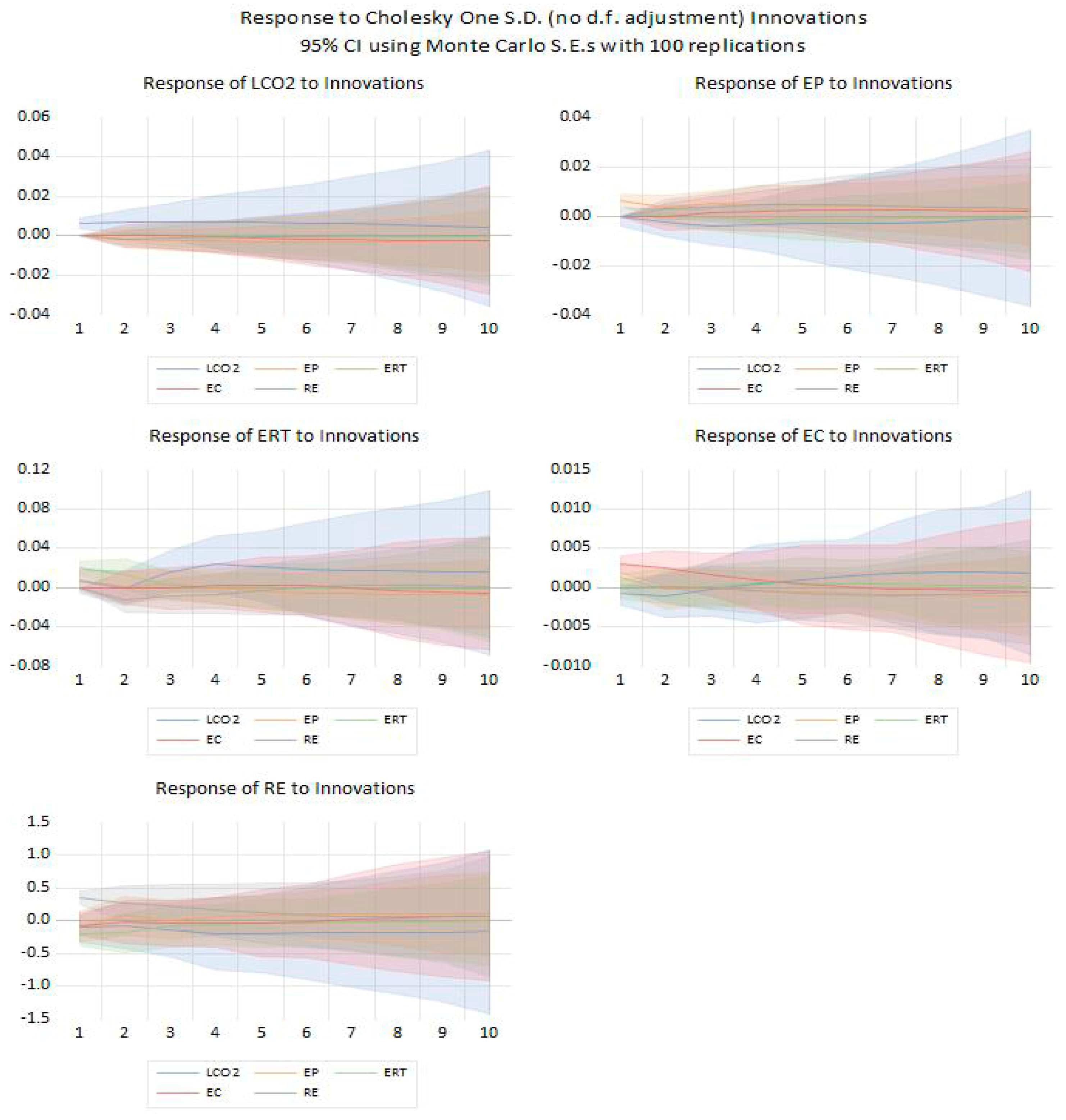
The impulse response functions provide additional insight into the dynamic adjustment process (Figure A1 in Appendix A). The results indicate that a shock to CO₂ emissions produces immediate and significant changes in energy efficiency, environmentally related tax, renewable energy, and non-renewable energy consumption over the next 10 years. This is because all variables return to zero within the 10-year period, and the wide confidence intervals reflect uncertainty about the long-run effectiveness of energy efficiency, environmentally related taxes, and renewable energy in mitigating carbon emissions. The output suggests that the system does not automatically adjust to CO₂ shocks. Effective policies may be required to accelerate the transition towards sustainable energy.

Table 8. Granger causality test results.

Dependent Variable			Short-Run Causality			Long Run (t-Statistics)
	DLCO2	DLEE	DLERT	DLEC	DLRE	ECT
DLCO2		7.580 ** (0.010)	5.358 ** (0.028)	3.596 * (0.068)	0.516 (0.478)	−0.283 *** (5.09)
DLEE	0.087 (0.769)		7.025 ** (0.040)	3.110 * (0.080)	5.040 ** (0.034)	−0.649 *** (4.67)
DLERT	5.923 ** (0.021)	0.941 (0.271)		4.820 ** (0.036)	0.814 (0.607)	−0.491 *** (3.68)
DLEC	0.482 (0.493)	5.370 ** (0.022)	1.817 0.110		1.817 (0.687)	0.563 (0.89)
DRE	1.881 (0.181)	8.582 *** (0.004)	3.430 * (0.051)	6.746 ** (0.030)		0.170 (1.07)

Notes: ***, **, * denote statistical significance at the 1%, 5%, and 1% levels, respectively. ${\mathrm{E}\mathrm{C}\mathrm{T}}_{\mathrm{t}-1}$ values are obtained via the t-statistics, short-run causalities are obtained via the F-statistics. The columns represent the dependent variables, while the rows denote the independent variables H₀: $\mathrm{X}$ does not Granger-cause $\mathrm{Y}$. H₁: $\mathrm{X}$ Granger-causes Y.

presents the VECM Granger causality results, indicating both short-run and long-run causal relationships. Energy efficiency (LEE) and environmentally related taxes (LERTs) Granger-cause CO₂ emissions in the short run at the 1% and 5% levels, respectively. Non-renewable energy consumption (LEC) is weakly significant at the 10% level, whereas renewable energy (LRE) does not Granger-cause LCO₂. The study of [86] revealed similar outcomes. Notably, LEE Granger-causes LEC and LRE, indicating that efficiency improvements lead to lower consumption of non-renewable energy and increase the adoption of renewables.

Bidirectional causality between LERT and CO₂ emissions is confirmed; taxes may lead to lower emissions (forward causation), while higher emissions may prompt policymakers to adjust their tax policy to curb emissions. This bidirectional relationship creates a feedback loop in which taxation and emissions influence each other. This feedback loop introduces simultaneity, making it difficult to determine the true effect of ERT on mitigating emissions in the long run and potentially explaining the inconclusive findings on emission mitigation.

In the long run, the negative and significant error correction terms (ECTs) at the 1% level for LCO₂, LEE, and LERT indicate that these variables converge to long-run equilibrium from short-run deviations. These results establish a coherent long-run cointegrating system among CO₂ emissions, LEE, and LERT. In contrast, the ECTs for LEC and LRE are positive and statistically insignificant, suggesting weak exogeneity.

Importantly, Granger causality tests are not definitive proof of causation; they provide statistical evidence of predictive relationships (a statistical transmission mechanism) among the variables [87]. Researchers should always consider other factors and conduct additional studies to confirm structural causal links.

Table 9. ARDL bounds test results.

F-Bounds Test		Null Hypothesis: No levels of relationship
Test Statistic	Value	Significance.	I(0)	I(1)
F-statistic	6.233	10%	1.9	3.01
Number of regressors (k)	4	5%	2.26	3.48
		2.50%	2.62	3.9
		1%	3.07	4.44
t-Bounds Test		Null Hypothesis: No levels of relationship
Test Statistic	Value	Significance.	I(0)	I(1)
t-statistic	−6.384	10%	−1.62	−3.26
		5%	−1.95	−3.6
		2.50%	−2.24	−3.89
		1%	−2.58	−4.23

presents the results of the ARDL bounds cointegration test, which confirm the presence of a long-run relationship among the variables studied. Before performing the bounds test, the authors conducted unit root tests to ensure that all individual time series variables are stationary, meaning their statistical properties, including means and variances, do not change over time. ADF, PP, and KPSS unit root test results revealed that all variables were stationary after first differencing, satisfying the condition for a bounds cointegration test. The results as presented in Table 9 confirm the presence of a long-run relationship among the variables, as evidenced by the F-statistic of 6.233, which exceeds the critical values at the 10%, 5%, and 1% statistical significance levels [64,75].

The study conducted several post-diagnostics to confirm the validity and reliability of the results.

Table 10. Diagnostic tests.

Diagnostic Tests	F-Statistics	Probability
Breusch–Godfrey Serial Correlation LM Test:	0.361	0.704
Breusch–Pagan–Godfrey	0.347	0.968
Ramsey RESET	0.001	0.974
Harvey	9.217	0.208
Glejser	0.573	0.840
ARCH	0.008	0.926
CUSUM	Stable
CUSUM2	Stable

reports the diagnostic test results. The results reveal no evidence of serial correlation among CO₂ emissions, LEE, LERT, LRE, and LEC. The Breusch–Godfrey Serial Correlation LM test, with an F-statistic of 0.361 and a p-value of 0.704, indicates no serial correlation in the residuals.

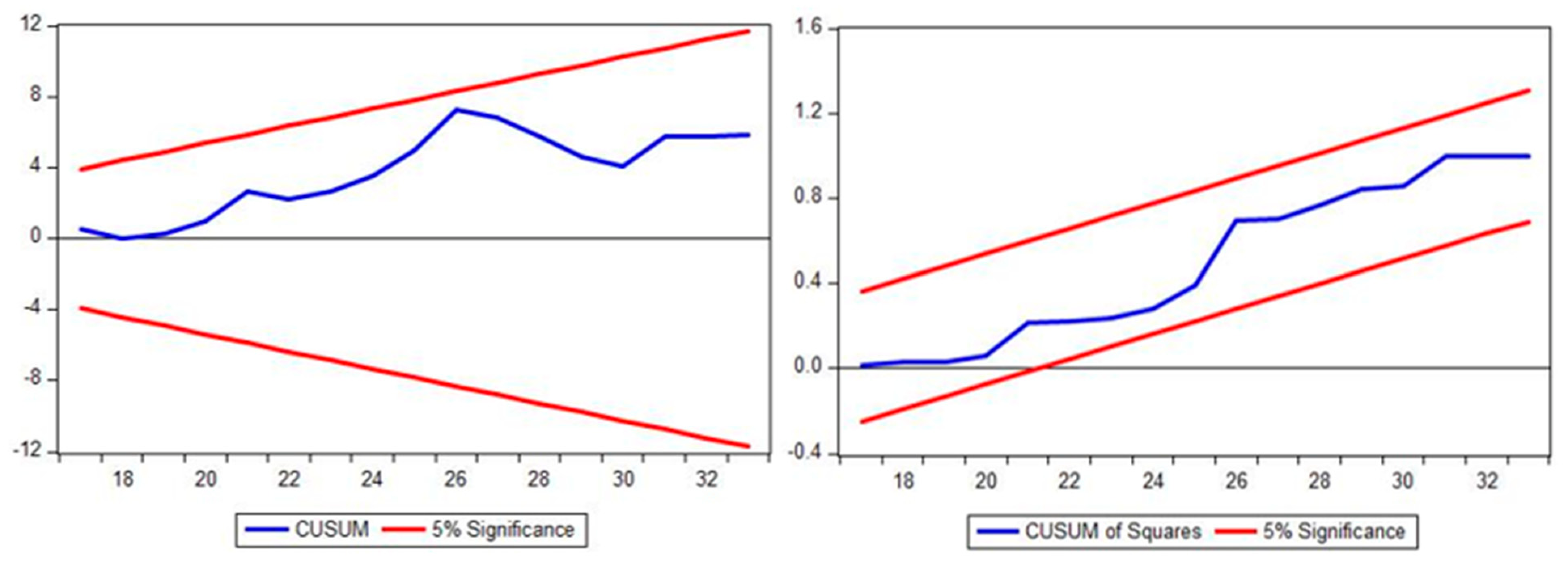
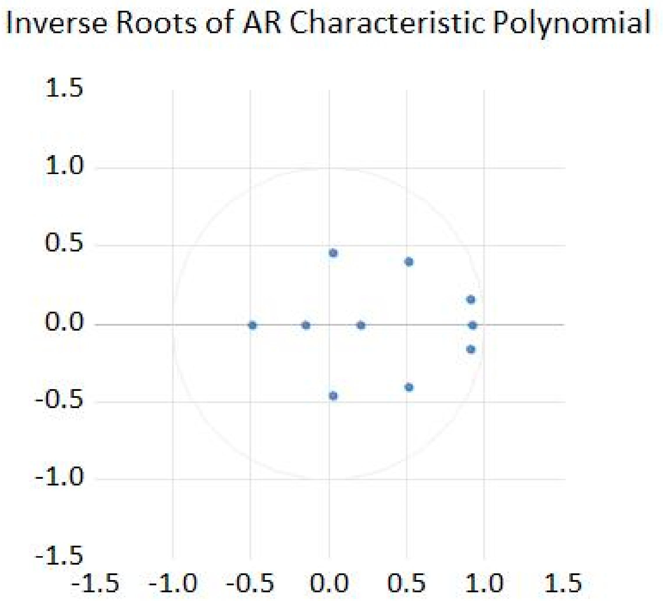
In Table 10, the Breusch–Pagan–Godfrey F-statistic is 0.347, with a probability of 0.968, suggesting that the error term’s variance is constant. The Ramsey RESET test confirms that the model’s functional form is correctly specified, with an F-statistic of 0.001 and a p-value of 0.974. Tests by Harvey (F-statistic = 9.217, probability value = 0.208) and Glejser (F-statistic = 0.573, probability value = 0.840) confirm that the variance of the residuals (differences between observed and predicted values) is constant across groups or levels, implying homoscedasticity. The autoregressive conditional heteroscedasticity (ARCH) test yields an F-statistic of 0.008 and a probability of 0.926, indicating the absence of conditional heteroscedasticity. Lastly, the CUSUM and CUSUM squares tests developed by [88,89] validate the model’s stability within the 5% critical limit, as shown in Figure 5. The stability of the ARDL model is further confirmed by the inverse roots of the characteristic polynomial (Figure A2 in the Appendix A). All inverse roots lie within the unit circle, indicating that the model is stable and satisfies the stationarity condition. Accordingly, the estimated coefficients are reliable and valid for policy implementation.

The study employed FMOLS and DOLS as alternative cointegration estimators to assess the sensitivity of the ARDL long-run results. The results are reported in

Table 11. Robustness tests.

Dependent Variable: LCO2 Emissions
	FMOLS			DOLS
Variable	Coefficient	Std. Error	t-Statistic	Coefficient	Std. Error	t-Statistic
LEE	−0.053	0.051	−1.035	−0.049	0.084	−0.585
LERT	−0.118 ***	0.034	−3.484	−0.117 **	0.048	−2.428
LEC	0.704 ***	0.086	8.099	0.698 ***	0.144	4.836
LRE	−0.008 *	0.004	−1.954	−0.008	0.007	−1.256

Note: *, **, and *** indicate statistical significance at the 10%, 5%, and 1% levels, respectively.

. In the long run, non-renewable energy consumption (LEC) has a positive and statistically significant effect on CO₂ emissions across ARDL, FMOLS, and DOLS, confirming that non-renewable energy consumption remains a major determinant of CO₂ emissions in Australia. This result is robust across all estimators. Energy efficiency (LEE) shows no statistically significant effect in the FMOLS and DOLS estimates, consistent with the ARDL result.

Likewise, the long-run effect of renewable energy (LRE) is not robust. The FMOLS result is marginally significant at the 10% level, whereas the DOLS estimate is statistically insignificant. These results may suggest that, in the long run, RE is not a primary climate-mitigating tool.

A notable discrepancy arises for environmentally related taxes (LERTs). Both the FMOLS and DOLS coefficients are negative and statistically significant, in sharp contrast to the ARDL bounds test, which provides no evidence of a long-run relationship. This discrepancy could be due to the long-run estimators’ sensitivity to lag-length selection, small sample sizes, or LERT’s mitigating role in emission reduction being more pronounced in fully cointegrated systems than in ARDL. However, because the ARDL bounds test is specifically suited for small samples and does not require all variables to be strictly I(1), the authors place key emphasis on the ARDL findings.

6. Conclusions and Policy Recommendations

This paper makes an important contribution to the literature on the relationships among energy efficiency, CO₂ emissions, environmentally related taxes, renewable energy, and non-renewable energy consumption in Australia from 1990 to 2020. The purpose is to identify the primary climate-mitigating factor in reducing Australia’s carbon emissions. These findings have significant policy implications for promoting sustainable energy adaptation and mitigating climate change.

First, the study emphasizes the critical role of energy efficiency in reducing CO₂ emissions and promoting a sustainable environment. The finding that a 1% increase in energy efficiency is negatively associated with CO₂ emissions in the short run underscores the importance of prioritizing energy efficiency measures. Sustaining these short-run gains through consistent policy frameworks will be critical for curbing long-run emissions. Second, the environmentally related tax (LERT) exhibits a negative association with CO₂ emissions in the short run, highlighting the importance of taxation as a policy tool to incentivize environmentally friendly practices. The long-run coefficient is statistically insignificant. Third, the study shows that an increase in renewable energy consumption is negatively associated with CO₂ emissions in the short run, underscoring the need to continue and expand investments in renewable energy sources as part of a sustainable energy strategy. In line with [29], reliance on energy imports will increase CO₂ emissions. Its long-run coefficient is statistically insignificant. Fourth, non-renewable energy consumption exhibits a strong positive association with CO₂ emissions, underscoring the urgency of transitioning away from fossil fuels. The research suggests that energy efficiency should be given the highest priority among the variables studied when transitioning from nonrenewable to green energy production and consumption. This prioritization is crucial for achieving sustainability goals.

Overall, the results of FMOLS and DOLS are consistent with those from the ARDL approach, although for environmentally related taxes, the results remain mixed. This highlights the need for careful interpretation of long-run coefficients for policy-relevant variables and supports the robustness of the findings while providing a more nuanced basis for policy recommendations. First, governments and international organizations should prioritize and promote energy efficiency measures across all sectors. This includes setting efficiency standards, offering incentives for energy-efficient technologies, and implementing energy-saving practices in industries, buildings, and transportation. Second, policymakers should consider implementing or enhancing environmental taxes to discourage CO₂ emissions and encourage sustainable practices. Revenue from such taxes can be reinvested in green initiatives. Third, Australia should encourage investment and provide incentives to develop and adopt renewable energy sources. This can include subsidies, feed-in tariffs, and supportive regulatory frameworks to facilitate the growth of clean energy.

Fourth, the country will need to develop a clear roadmap to phase out conventional energy sources, such as coal and oil, and transition to cleaner alternatives. This may include setting timelines for decommissioning fossil fuel power plants and promoting research and development of green technologies. Lastly, collaboration with international organizations and neighboring countries is necessary to align energy policies and tackle climate change collectively. Sharing best practices and facilitating technology transfers can accelerate progress toward sustainability. Moreover, establishing a robust monitoring and reporting system to track progress in energy efficiency, renewable energy adoption, and CO₂ emissions reduction should be considered. Regularly updating and assessing policy measures will help ensure that goals are met.

The findings of this study underscore the importance of holistic policy approaches that prioritize energy efficiency, renewable energy adoption, environmental taxation, and the phase-out of conventional energy sources. These policies are essential for reducing CO₂ emissions and promoting a green, sustainable environment in Australia. They can serve as a valuable reference for other countries facing similar challenges as they pursue a sustainable energy future.

One of the primary limitations of this study is its reliance on historical data from 1990 to 2020. The data may not fully capture recent developments in energy consumption and environmental policies. Future research should incorporate more up-to-date data to provide a more accurate picture of the current situation. The study employs the dynamic ARDL model to analyze relationships among variables. While this model is valuable, it relies on certain assumptions, and the accuracy of its results depends on the validity of those assumptions. Sensitivity analysis and further robustness tests can help address some of these concerns. In addition, the present research focuses on Australia, which may have unique characteristics and policies. Generalizing the findings to other countries or regions should be done cautiously, as the effectiveness of energy efficiency, taxation, and renewable energy policies can vary significantly depending on local factors. Finally, the study identifies predictive causal associations between variables but does not establish structural causality, which reflects the actual causal effect. Future work could explore causality more rigorously by addressing potential endogeneity that might affect the observed relationships.

References

1. Hassan, T.; Song, H.; Khan, Y.; Kirikkaleli, D. Energy efficiency a source of low carbon energy sources? Evidence from 16 high-income OECD economies. Energy 2022, 243, 123063. [Google Scholar] [CrossRef] [Scilit]
2. Liu, F.; Khan, Y.; Hassan, T. Does excessive energy utilization and expansion of urbanization increase carbon dioxide emission in Belt and Road economies? Environ. Sci. Pollut. Res. 2023, 30, 60080–60105. [Google Scholar] [CrossRef] [Scilit] [PubMed]
3. Khan, Y.; Oubaih, H.; Hassan, T. Assessing the Role of Energy Depletion and Energy Import with Carbon Dioxide Emissions in Belt and Road Countries. J. Knowl. Econ. 2023, 15, 7852–7872. [Google Scholar] [CrossRef] [Scilit]
4. Shahbaz, M.; Solarin, S.A.; Sbia, R.; Bibi, S. Does energy intensity contribute to CO2 emissions? A trivariate analysis in selected African countries. Ecol. Indic. 2015, 50, 215–224. [Google Scholar] [CrossRef] [Scilit]
5. Wang, F.; Zhang, Z. Decoupling economic growth from energy consumption in top five energy consumer economies: A technological and urbanization perspective. J. Clean. Prod. 2022, 357, 131890. [Google Scholar] [CrossRef] [Scilit]
6. Khan, Y.; Bin, Q.; Hassan, T. The impact of climate changes on agriculture export trade in Pakistan: Evidence from time-series analysis. Growth Change 2019, 50, 1568–1589. [Google Scholar] [CrossRef] [Scilit]
7. An, R.; Zhu, G. Clustering of economic efficiency of urban energy carbon emissions based on decoupling theory. Energy Rep. 2022, 8, 9569–9575. [Google Scholar] [CrossRef] [Scilit]
8. Hubacek, K.; Chen, X.; Feng, K.; Wiedmann, T.; Shan, Y. Evidence of decoupling consumption-based CO2 emissions from economic growth. Adv. Appl. Energy 2021, 4, 100074. [Google Scholar] [CrossRef] [Scilit]
9. Charfeddine, L.; Kahia, M. Do information and communication technology and renewable energy use matter for carbon dioxide emissions reduction? Evidence from the Middle East and North Africa region. J. Clean. Prod. 2021, 327, 129410. [Google Scholar] [CrossRef] [Scilit]
10. Wu, J.; Zhu, Q.; Liang, L. CO2 emissions and energy intensity reduction allocation over provincial industrial sectors in China. Appl. Energy 2016, 166, 282–291. [Google Scholar] [CrossRef] [Scilit]
11. Arroyo M., F.R.; Miguel, L.J. The trends of the energy intensity and CO2 emissions related to final energy consumption in Ecuador: Scenarios of national and worldwide strategies. Sustainability 2019, 12, 20. [Google Scholar] [CrossRef] [Scilit]
12. GCP. Carbon Emissions; Global Carbon Project: Canberra, Australia, 2023; Available online: https://globalcarbonatlas.org/emissions/carbon-emissions/ (accessed on 15 August 2023).
13. Malmedal, K.; Kroposki, B.; Sen, P.K. Energy Policy Act of 2005 and its impact on renewable energy applications in USA. In 2007 IEEE Power Engineering Society General Meeting; IEEE: Piscataway, NJ, USA, 2007; pp. 1–8. [Google Scholar]
14. Kilinc-Ata, N. The evaluation of renewable energy policies across EU countries and US states: An econometric approach. Energy Sustain. Dev. 2016, 31, 83–90. [Google Scholar] [CrossRef] [Scilit]
15. Oesingmann, K. The effect of the European Emissions Trading System (EU ETS) on aviation demand: An empirical comparison with the impact of ticket taxes. Energy Policy 2022, 160, 112657. [Google Scholar] [CrossRef] [Scilit]
16. Shrestha, R.M.; Pradhan, S. Co-benefits of CO2 emission reduction in a developing country. Energy Policy 2010, 38, 2586–2597. [Google Scholar] [CrossRef] [Scilit]
17. Danish; Baloch, M.A.; Mahmood, N.; Zhang, J.W. Effect of natural resources, renewable energy and economic development on CO2 emissions in BRICS countries. Sci. Total Environ. 2019, 678, 632–638. [Google Scholar] [CrossRef] [Scilit] [PubMed]
18. Zhou, S.; Shi, M.; Li, N.; Yuan, Y. Impacts of Carbon Tax Policy on CO2 Mitigation and Economic Growth in China. Adv. Clim. Change Res. 2011, 2, 124–133. [Google Scholar] [CrossRef] [Scilit]
19. Cavallaro, F.; Danielis, R.; Nocera, S.; Rotaris, L. Should BEVs be subsidized or taxed? A European perspective based on the economic value of CO2 emissions. Transp. Res. Part D Transp. Environ. 2018, 64, 70–89. [Google Scholar] [CrossRef] [Scilit]
20. Nong, D.; Simshauser, P.; Nguyen, D.B. Greenhouse gas emissions vs CO2 emissions: Comparative analysis of a global carbon tax. Appl. Energy 2021, 298, 117223. [Google Scholar] [CrossRef] [Scilit]
21. Calderón, S.; Alvarez, A.C.; Loboguerrero, A.M.; Arango, S.; Calvin, K.; Kober, T.; Daenzer, K.; Fisher-Vanden, K. Achieving CO2 reductions in Colombia: Effects of carbon taxes and abatement targets. Energy Econ. 2016, 56, 575–586. [Google Scholar] [CrossRef] [Scilit]
22. Wolde-Rufael, Y.; Mulat-Weldemeskel, E. The moderating role of environmental tax and renewable energy in CO2 emissions in Latin America and Caribbean countries: Evidence from method of moments quantile regression. Environ. Chall. 2022, 6, 100412. [Google Scholar] [CrossRef] [Scilit]
23. Yang, Z.; Zhang, M.; Liu, L.; Zhou, D. Can renewable energy investment reduce carbon dioxide emissions? Evidence from scale and structure. Energy Econ. 2022, 112, 106181. [Google Scholar] [CrossRef] [Scilit]
24. Balsalobre-Lorente, D.; Driha, O.M.; Leitão, N.C.; Murshed, M. The carbon dioxide neutralizing effect of energy innovation on international tourism in EU-5 countries under the prism of the EKC hypothesis. J. Environ. Manag. 2021, 298, 113513. [Google Scholar] [CrossRef] [Scilit] [PubMed]
25. Tamura, H.; Abe, M.; Tomiyama, S.; Hatono, I. Evaluating the Effectiveness of Carbon Tax for Total Emission Control of Carbon Dioxide:—Systems Analysis of a Dynamic Environmental-Economic Model. IFAC Proc. Vol. 1998, 31, 581–586. [Google Scholar]
26. Tajudeen, I.A.; Wossink, A.; Banerjee, P. How significant is energy efficiency to mitigate CO2 emissions? Evidence from OECD countries. Energy Econ. 2018, 72, 200–221. [Google Scholar] [CrossRef] [Scilit]
27. Gonçalves, R.; Menezes, F. The carbon tax and the crisis in Australia’s National Electricity Market. Energy Econ. 2024, 133, 107522. [Google Scholar] [CrossRef] [Scilit]
28. Murad, S.M.W.; Rahman, A.; Mohsin, A.K.M. From policy to progress: Environmental taxation to mitigate air pollution in OECD countries. J. Environ. Manag. 2025, 374, 124143. [Google Scholar] [CrossRef] [Scilit] [PubMed]
29. Sarkodie, S.A.; Strezov, V. Assessment of contribution of Australia’s energy production to CO2 emissions and environmental degradation using statistical dynamic approach. Sci. Total Environ. 2018, 639, 888–899. [Google Scholar] [CrossRef] [Scilit] [PubMed]
30. Rai, P.; Gupta, P.; Saini, N.; Tiwari, A.K. Assessing the impact of renewable energy and non-renewable energy use on carbon emissions: Evidence from select developing and developed countries. Environ. Dev. Sustain. 2023, 27, 3059–3080. [Google Scholar] [CrossRef] [Scilit]
31. Ehigiamusoe, K.U.; Dogan, E. The role of interaction effect between renewable energy consumption and real income in carbon emissions: Evidence from low-income countries. Renew. Sustain. Energy Rev. 2022, 154, 111883. [Google Scholar] [CrossRef] [Scilit]
32. Liu, F.; Khan, Y.; Marie, M. Carbon neutrality challenges in Belt and Road countries: What factors can contribute to CO2 emissions mitigation? Environ. Sci. Pollut. Res. 2022, 30, 14884–14901. [Google Scholar] [CrossRef] [Scilit] [PubMed]
33. IEA. Data and Statistics; International Energy Agency: Paris, France, 2023; Available online: https://www.iea.org/data-and-statistics (accessed on 26 April 2023).
34. Wei, F.; Zhang, X.; Chu, J.; Yang, F.; Yuan, Z. Energy and environmental efficiency of China’s transportation sectors considering CO2 emission uncertainty. Transp. Res. Part D Transp. Environ. 2021, 97, 102955. [Google Scholar] [CrossRef] [Scilit]
35. Feng, Y.; Liu, Q.; Li, Y.; Yang, J.; Dong, Z. Energy efficiency and CO2 emission comparison of alternative powertrain solutions for mining haul truck using integrated design and control optimization. J. Clean. Prod. 2022, 370, 133568. [Google Scholar] [CrossRef] [Scilit]
36. Lee, M.; Lee, H.; Seo, C.; Lee, J.; Lee, J.W. Enhanced energy efficiency and reduced CO2 emissions by hybrid heat integration in dimethyl carbonate production systems. Sep. Purif. Technol. 2022, 287, 120598. [Google Scholar] [CrossRef] [Scilit]
37. Pylsy, P.; Lylykangas, K.; Kurnitski, J. Buildings’ energy efficiency measures effect on CO2 emissions in combined heating, cooling and electricity production. Renew. Sustain. Energy Rev. 2020, 134, 110299. [Google Scholar] [CrossRef] [Scilit]
38. Kamal, A.; Al-Ghamdi, S.G.; Koç, M. Role of energy efficiency policies on energy consumption and CO2 emissions for building stock in Qatar. J. Clean. Prod. 2019, 235, 1409–1424. [Google Scholar] [CrossRef] [Scilit]
39. Bhadbhade, N.; Zuberi, M.J.S.; Patel, M.K. A bottom-up analysis of energy efficiency improvement and CO2 emission reduction potentials for the swiss metals sector. Energy 2019, 181, 173–186. [Google Scholar] [CrossRef] [Scilit]
40. Martínez-Moya, J.; Vazquez-Paja, B.; Gimenez Maldonado, J.A. Energy efficiency and CO2 emissions of port container terminal equipment: Evidence from the Port of Valencia. Energy Policy 2019, 131, 312–319. [Google Scholar] [CrossRef] [Scilit]
41. Mehmood Mirza, F.; Sinha, A.; Rehman Khan, J.; Kalugina, O.A.; Wasif Zafar, M. Impact of energy efficiency on CO2 Emissions: Empirical evidence from developing countries. Gondwana Res. 2022, 106, 64–77. [Google Scholar] [CrossRef] [Scilit]
42. Li, G.; Zakari, A.; Tawiah, V. Energy resource melioration and CO2 emissions in China and Nigeria: Efficiency and trade perspectives. Resour. Policy 2020, 68, 101769. [Google Scholar] [CrossRef] [Scilit]
43. Fei, R.; Lin, B. The integrated efficiency of inputs–outputs and energy—CO2 emissions performance of China’s agricultural sector. Renew. Sustain. Energy Rev. 2017, 75, 668–676. [Google Scholar] [CrossRef] [Scilit]
44. Kazemian, S.; Zaman, R.; Foroughi, B.; Ghobakhloo, M. Determining the carbon footprint of Australia’s electricity, gas, water and waste services sector. Manag. Environ. Qual. Int. J. 2025, 37, 21–45. [Google Scholar] [CrossRef] [Scilit]
45. Bakirtas, T.; Akpolat, A.G. The relationship between energy consumption, urbanization, and economic growth in new emerging-market countries. Energy 2018, 147, 110–121. [Google Scholar] [CrossRef] [Scilit]
46. Hassan, M.; Oueslati, W.; Rousselière, D. Environmental taxes, reforms and economic growth: An empirical analysis of panel data. Econ. Syst. 2020, 44, 100806. [Google Scholar] [CrossRef] [Scilit]
47. Bashir, M.F.; Ma, B.; Shahbaz, M.; Shahzad, U.; Vo, X.V. Unveiling the heterogeneous impacts of environmental taxes on energy consumption and energy intensity: Empirical evidence from OECD countries. Energy 2021, 226, 120366. [Google Scholar] [CrossRef] [Scilit]
48. Yunzhao, L. Modelling the role of eco innovation, renewable energy, and environmental taxes in carbon emissions reduction in E−7 economies: Evidence from advance panel estimations. Renew. Energy 2022, 190, 309–318. [Google Scholar] [CrossRef] [Scilit]
49. Sun, J.; Zhang, X.-B.; Liu, Y.; Zheng, X. Pass-through of diesel taxes and the effect on carbon emissions: Evidence from China. J. Environ. Manag. 2022, 321, 115857. [Google Scholar] [CrossRef] [Scilit] [PubMed]
50. Li, S.; Jia, N.; Chen, Z.; Du, H.; Zhang, Z.; Bian, B. Multi-objective optimization of environmental tax for mitigating air pollution and greenhouse gas. J. Manag. Sci. Eng. 2022, 7, 473–488. [Google Scholar] [CrossRef] [Scilit]
51. Sheraz, M.; Qin, Q.; Mumtaz, M.Z. Energy transition in OECD countries: Catalyzing governance quality for SDG 7 attainment. Energy Policy 2024, 194, 114315. [Google Scholar] [CrossRef] [Scilit]
52. Chen, Z.; Huang, W.; Zheng, X. The decline in energy intensity: Does financial development matter? Energy Policy 2019, 134, 110945. [Google Scholar] [CrossRef] [Scilit]
53. Liu, G.; Yang, Z.; Zhang, F.; Zhang, N. Environmental tax reform and environmental investment: A quasi-natural experiment based on China’s Environmental Protection Tax Law. Energy Econ. 2022, 109, 106000. [Google Scholar] [CrossRef] [Scilit]
54. Solorio, I.; Bocquillon, P. EU renewable energy policy: A brief overview of its history and evolution. In A Guide to EU Renewable Energy Policy; Edwad Elgar: Worcester, UK, 2017; pp. 23–42. [Google Scholar]
55. Okioga, I.T.; Wu, J.; Sireli, Y.; Hendren, H. Renewable energy policy formulation for electricity generation in the United States. Energy Strategy Rev. 2018, 22, 365–384. [Google Scholar] [CrossRef] [Scilit]
56. Beken, M.; Hangun, B.; Eyecioglu, O. Classification of turkey among european countries by years in terms of energy efficiency, total renewable energy, energy consumption, greenhouse gas emission and energy import dependency by using machine learning. In 2019 8th International Conference on Renewable Energy Research and Applications (ICRERA); IEEE: Piscataway, NJ, USA, 2019; pp. 951–956. [Google Scholar]
57. Jeon, H. CO2 emissions, renewable energy and economic growth in the US. Electr. J. 2022, 35, 107170. [Google Scholar] [CrossRef] [Scilit]
58. Khan, Y.; Oubaih, H.; Elgourrami, F.Z. The effect of renewable energy sources on carbon dioxide emissions: Evaluating the role of governance, and ICT in Morocco. Renew. Energy 2022, 190, 752–763. [Google Scholar] [CrossRef] [Scilit]
59. Rahman, M.M.; Alam, K.; Velayutham, E. Reduction of CO2 emissions: The role of renewable energy, technological innovation and export quality. Energy Rep. 2022, 8, 2793–2805. [Google Scholar] [CrossRef] [Scilit]
60. Abbasi, K.R.; Adedoyin, F.F.; Abbas, J.; Hussain, K. The impact of energy depletion and renewable energy on CO2 emissions in Thailand: Fresh evidence from the novel dynamic ARDL simulation. Renew. Energy 2021, 180, 1439–1450. [Google Scholar] [CrossRef] [Scilit]
61. Le, T.H. Connectedness between nonrenewable and renewable energy consumption, economic growth and CO2 emission in Vietnam: New evidence from a wavelet analysis. Renew. Energy 2022, 195, 442–454. [Google Scholar] [CrossRef] [Scilit]
62. Chen, C.; Pinar, M.; Stengos, T. Renewable energy and CO2 emissions: New evidence with the panel threshold model. Renew. Energy 2022, 194, 117–128. [Google Scholar] [CrossRef] [Scilit]
63. WDI. World Development Indicators Database; World Bank: Washington, DC, USA, 2023; Available online: https://databank.worldbank.org/reports.aspx?source=world-development-indicators (accessed on 2 February 2023).
64. Pesaran, M.H.; Shin, Y.; Smith, R.J. Bounds testing approaches to the analysis of level relationships. J. Appl. Econom. 2001, 16, 289–326. [Google Scholar] [CrossRef] [Scilit]
65. Dickey, D.A.; Fuller, W.A. Distribution of the estimators for autoregressive time series with a unit root. J. Am. Stat. Assoc. 1979, 74, 427–431. [Google Scholar] [CrossRef] [Scilit]
66. Phillips, P.C.B.; Xiao, Z. A Primer on Unit Root Testing. J. Econ. Surv. 1998, 12, 423–470. [Google Scholar] [CrossRef] [Scilit]
67. Shin, Y.; Schmidt, P. The KPSS stationarity test as a unit root test. Econ. Lett. 1992, 38, 387–392. [Google Scholar] [CrossRef] [Scilit]
68. Phillips, P.C.; Perron, P. Testing for a unit root in time series regression. Biometrika 1988, 75, 335–346. [Google Scholar] [CrossRef] [Scilit]
69. Pesaran, M.H.; Shin, Y.; Smith, R.P. Pooled mean group estimation of dynamic heterogeneous panels. J. Am. Stat. Assoc. 1999, 94, 621–634. [Google Scholar] [CrossRef]
70. Dritsaki, M.; Dritsaki, C.; Idziak, E. Nexus Between Renewable, Non-Renewable, Nuclear Energy Consumption and Economic Growth in Five Developing and Developed Countries: A Cobb–Douglas Production Function Analysis. Energies 2026, 19, 2634. [Google Scholar] [CrossRef] [Scilit]
71. Bekoe, B.B.; Chen, J.; Tougem, T.O.; Nketiah, E.; Sakuwunda, K. Does domestic investment matter? A multivariate time series analysis of the energy-CO2 emission-growth nexus in Ghana. Environ. Sci. Pollut. Res. Int. 2023, 30, 49536–49550. [Google Scholar] [CrossRef] [Scilit] [PubMed]
72. Abdi, A.H.; Zaidi, M.A.S.; Halane, D.R.; Warsame, A.A. Asymmetric effects of foreign direct investment and trade openness on economic growth in Somalia: Evidence from a non-linear ARDL approach. Cogent Econ. Financ. 2024, 12, 2305010. [Google Scholar] [CrossRef] [Scilit]
73. Johansen, S.; Juselius, K. Maximum likelihood estimation and inference on cointegration—With appucations to the demand for money. Oxf. Bull. Econ. Stat. 1990, 52, 169–210. [Google Scholar] [CrossRef] [Scilit]
74. Engle, R.F.; Granger, C.W. Co-integration and error correction: Representation, estimation, and testing. Econ. J. Econ. Soc. 1987, 55, 251–276. [Google Scholar] [CrossRef] [Scilit]
75. Rahman, M.M.; Kashem, M.A. Carbon emissions, energy consumption and industrial growth in Bangladesh: Empirical evidence from ARDL cointegration and Granger causality analysis. Energy Policy 2017, 110, 600–608. [Google Scholar] [CrossRef] [Scilit]
76. Xuan, V.N. Determinants of Environmental Pollution in China: Novel Findings from ARDL Method. Environ. Health Insights 2024, 18, 1–29. [Google Scholar] [CrossRef] [Scilit] [PubMed]
77. Obeng-Amponsah, W.; Owusu, E. Foreign direct investment, technological transfer, employment generation and economic growth: New evidence from Ghana. Int. J. Emerg. Mark. 2023, 20, 2088–2109. [Google Scholar] [CrossRef] [Scilit]
78. Pedroni, P. Critical Values for Cointegration Tests in Heterogeneous Panels with Multiple Regressors. Oxf. Bull. Econ. Stat. 1999, 61, 653–670. [Google Scholar] [CrossRef]
79. Kent, A.; Mercer, D. Australia’s mandatory renewable energy target (MRET): An assessment. Energy Policy 2006, 34, 1046–1062. [Google Scholar] [CrossRef] [Scilit]
80. Nguyen, J.H.; Truong, C.; Zhang, B. The price of carbon risk: Evidence from the Kyoto Protocol ratification. J. Environ. Econ. Manag. 2025, 130, 103118. [Google Scholar] [CrossRef] [Scilit]
81. Anwar, A.; Siddique, M.; Dogan, E.; Sharif, A. The moderating role of renewable and non-renewable energy in environment-income nexus for ASEAN countries: Evidence from Method of Moments Quantile Regression. Renew. Energy 2021, 164, 956–967. [Google Scholar] [CrossRef] [Scilit]
82. Pata, U.K. Renewable and non-renewable energy consumption, economic complexity, CO2 emissions, and ecological footprint in the USA: Testing the EKC hypothesis with a structural break. Environ. Sci. Pollut. Res. 2021, 28, 846–861. [Google Scholar] [CrossRef] [Scilit] [PubMed]
83. Khan, Y.; ShuKai, C.; Hassan, T.; Kootwal, J.; Khan, M.N. The links between renewable energy, fossil energy, terrorism, economic growth and trade openness: The case of Pakistan. SN Bus. Econ. 2021, 1, 115. [Google Scholar] [CrossRef] [Scilit]
84. Pata, U.K.; Caglar, A.E. Investigating the EKC hypothesis with renewable energy consumption, human capital, globalization and trade openness for China: Evidence from augmented ARDL approach with a structural break. Energy 2021, 216, 119220. [Google Scholar] [CrossRef] [Scilit]
85. Yuping, L.; Ramzan, M.; Xincheng, L.; Murshed, M.; Awosusi, A.A.; Bah, S.I.; Adebayo, T.S. Determinants of carbon emissions in Argentina: The roles of renewable energy consumption and globalization. Energy Rep. 2021, 7, 4747–4760. [Google Scholar] [CrossRef] [Scilit]
86. Khan, Y.; Oubaih, H.; Elgourrami, F.Z. The role of private investment in ICT on carbon dioxide emissions (CO2) mitigation: Do renewable energy and political risk matter in Morocco? Environ. Sci. Pollut. Res. 2022, 29, 52885–52899. [Google Scholar] [CrossRef] [Scilit] [PubMed]
87. Tutar, H.; Štreimikienė, D.; Kyriakopoulos, G.L. Short-Run Statistical Interactions Between Nuclear and Renewable Energy Production in the EU27: A Bivariate VAR Analysis (1990–2022). Energies 2026, 19, 2628. [Google Scholar] [CrossRef] [Scilit]
88. Brown, R.L.; Durbin, J.; Evans, J.M. Techniques for testing the constancy of regression relationships over time. J. R. Stat. Soc. Ser. B Stat. Methodol. 1975, 37, 149–163. [Google Scholar] [CrossRef] [Scilit]
89. Pesaran, M.H.; Pesaran, B. Working with Microfit 4.0: Interactive Econometric Analysis; Oxford University Press: Oxford, UK, 1997. [Google Scholar]
Figure 1. The historical trend of CO2 emissions per capita in Australia from 1850 to 2020. Source: Global Carbon Project [12], (https://ourworldindata.org/co2/country/australia) (accessed on 15 August 2023).
Energies 19 03812 g001
Figure 2. CO2 emissions by energy source in Australia between 1990 and 2020. Source: International Energy Agency [33], authors’ calculations.
Energies 19 03812 g002
Figure 3. Total energy consumption by sectors in Australia between 1990 and 2020. Source: International Energy Agency [33], authors’ calculations.
Energies 19 03812 g003
Figure 4. Econometric strategy [64].
Energies 19 03812 g004
Figure 5. CUSUM and CUSUM squares.
Energies 19 03812 g005