A Source-Load-Storage Alternating Coordinated Low-Carbon Economic Dispatch Method with Response-Gap Negative-Feedback Dual Incentives

Abstract

High-penetration renewable energy integration intensifies net-load fluctuations, renewable energy curtailment, and carbon-emission control challenges in power system dispatch. To improve low-carbon operation and source-load-storage coordination, this study proposes a two-layer alternating coordinated dispatch method with response-gap negative-feedback dual incentives. The dispatch-side layer jointly optimizes thermal generation, wind and photovoltaic power, carbon capture and storage, and ladder-type carbon trading, while the load-storage layer coordinates demand response and energy storage through peak-shaving and renewable-accommodation incentives. Unlike static incentives or dynamic schemes driven only by demand indices, the proposed mechanism updates incentive prices according to the deviation between dispatch-side expected response and load-storage-side realized response. The reconstructed net load is then fed back to the dispatch side, forming a closed-loop alternating coordination process. A typical-day case study shows that, compared with Scenario 1, the proposed method reduces the dispatch-side operating cost by 2.89% and net carbon emissions by 20.4%, while increasing the overall renewable energy accommodation rate by approximately 21.5 percentage points. Sensitivity and uncertainty tests further indicate that the main economic, emission-reduction, and renewable-accommodation benefits remain robust under different lower-layer preference weights and moderate demand-response uncertainty.

1. Introduction

Against the backdrop of carbon-peaking and carbon-neutrality goals, the installed capacity of renewable energy, especially wind and photovoltaic (PV) power, continues to increase, accelerating the transition toward clean and low-carbon power systems. However, the variability of high-penetration renewable generation complicates power balancing, increases the peak-shaving and ramping burden on thermal units, and may lead to wind and PV curtailment. Therefore, improving renewable energy accommodation and reducing net carbon emissions while maintaining economic operation have become key challenges in low-carbon economic dispatch [1,2,3,4].

Existing studies have enhanced system flexibility through thermal power peak shaving, energy storage, and wind-storage coordination. Reference [5] proposed a collaborative optimization method integrating load-side regulation with thermal power deep peak shaving, demonstrating that the coordinated use of source- and load-side peak-regulation resources can reduce renewable energy curtailment and improve the economics of deep peak shaving. References [6,7] examined thermal power regulation and coordinated wind-storage planning under renewable uncertainty, confirming that thermal flexibility and energy storage are effective in smoothing renewable energy fluctuations and reducing curtailment. Reference [8] proposed a two-stage day-ahead and intraday dispatch strategy to improve energy storage utilization, while Reference [9] coordinated energy storage and wind power to balance economic, low-carbon, and operational objectives. Nevertheless, these studies mainly focus on source-side regulation or storage optimization, with limited consideration of the coordination between adjustable loads and source-side low-carbon dispatch.

Demand response provides additional flexibility by shifting electricity consumption to support peak shaving, valley filling, and renewable energy accommodation. Reference [10] coordinated thermal power, energy storage, and demand response to enhance system regulation capability. More recently, NILM-based energy management methods have been proposed to infer appliance-level consumption from aggregated smart-meter data and integrate such information into robust hybrid microgrid scheduling under renewable uncertainty [11]. Such NILM-based methods provide appliance-level information for improving demand response scheduling, whereas the present study focuses on dispatch-level coordination using aggregated demand response and energy storage resources. References [12,13,14] further showed that coordinating demand response with energy storage can reduce operating costs and carbon emissions while smoothing the net-load curve. However, most existing approaches rely on static incentive prices or single-response schemes and therefore cannot dynamically adjust incentive signals according to peak-shaving demand, renewable accommodation requirements, and actual response performance. As a result, the response may be insufficient, excessive, or temporally mismatched.

Carbon capture and storage (CCS) and carbon trading are also important instruments for reducing the net emissions of thermal power systems. Reference [15] verified the emission-reduction and regulation benefits of CCS in systems with energy storage. Reference [16] improved CCS flexibility by coupling liquid-storage CCS with waste-heat recovery, while Reference [17] examined the synergy between carbon capture and demand response. References [18,19,20] investigated the coordination of wind power, flexible carbon-capture power plants, generalized energy storage, and ladder-type carbon trading. References [21,22] further incorporated green certificates and carbon trading into source-load coordinated dispatch. Although these studies demonstrate the benefits of coordinating CCS, flexible resources, and market mechanisms, they mainly model emission reduction and carbon constraints from the source-side perspective. The transmission of low-carbon dispatch and renewable accommodation requirements to the load-storage side remains insufficiently addressed. A structured comparison of previous studies on source-load-storage coordination, CCS, and demand response is provided in Appendix C (

Table A2. Literature History on Source-Load-Storage Coordination, CCS, and Demand Response.

Category	Representative Refs.	Main Focus	Main Limitation	Implication for This Work
System and planning background	[1,2,3,4]	New power systems, source-storage-load planning, and renewable integration challenges	Mostly review-level or planning-level discussion, with limited dispatch-side closed-loop coordination	Provides the system background and motivates closed-loop source-load-storage coordination
Source-load-storage coordination	[8,9,10,23,26,30]	Storage-assisted load shifting, source-load coupling, and low-carbon scheduling with flexible demand	Often relies on static coordination or one-way adjustment; explicit response correction is limited	Motivates the alternating source-load-storage framework with iterative feedback
CCS and carbon trading	[13,15,16,17,18,19,20,21,22,28,29]	CCS operation, carbon capture flexibility, ladder-type carbon trading, and quota allocation	Mainly emphasizes source-side emission control; load-side flexibility and feedback coordination are still weak	Motivates the integration of CCS, carbon trading, and load-storage coordination in a closed loop
Demand response and incentive pricing	[11,12,14,24,25]	Demand response scheduling, bilevel pricing, static/dynamic incentives, and NILM-based demand response	Many studies use static incentives or do not explicitly correct realized response deviation	Motivates the proposed response-gap negative-feedback pricing mechanism

) to further clarify the research gap.

Source-load-storage dispatch also involves interactions among dispatch operators, energy storage operators, and users. References [23,24] modeled user response and grid–user interactions in low-carbon and bi-level dispatch frameworks. References [25,26] employed iterative coordination and price signals to guide user-side resources and demand response aggregators. Reference [27] developed a bi-level iterative algorithm to improve the solution efficiency of dynamic dispatch models. Although these studies confirm the applicability of hierarchical and iterative frameworks for describing dispatch-user interactions, recent bi-level dispatch models mainly focus on hierarchical decision-making or equilibrium-oriented price transmission between the system operator and users. Different from these studies, the proposed method does not aim to construct a strict Stackelberg equilibrium. Instead, it develops a decomposition-coordination alternating framework in which incentive prices and reconstructed net load are iteratively exchanged between the dispatch side and the load-storage side. Moreover, compared with incentive-based coordination approaches using static prices or demand-index-driven dynamic prices, the proposed mechanism introduces an actual response-deviation correction term, so that the incentive price is updated according to the gap between the expected response and the realized load-storage response, thereby forming closed-loop coordination among price updating, load-storage response, and source-side net-load feedback.

Motivated by the above research gap, this paper aims to develop a two-layer alternating coordinated low-carbon economic dispatch method based on response-gap negative-feedback dual incentives. The objective is to reduce dispatch-side operating cost, net carbon emissions, and renewable energy curtailment by improving the matching between dispatch-side regulation requirements and load-storage-side actual responses. In the proposed framework, peak-shaving, carbon-control, and renewable energy accommodation requirements are translated into dual incentive signals to guide demand response and energy storage operation. The reconstructed net load is then fed back to the dispatch side, forming a closed-loop process involving dispatch optimization, incentive price updating, load-storage response, and net-load feedback. The main novelty and contributions of this study are summarized as follows. First, a low-carbon-oriented dual-incentive framework is developed to separately characterize peak-shaving and renewable energy accommodation requirements, thereby transmitting dispatch-side regulation requirements to the load-storage side. Second, a response-gap negative-feedback pricing mechanism is proposed to update incentive prices according to the deviation between expected and actual responses. This mechanism increases prices when the response is insufficient and stabilizes or reduces them when the response is adequate, avoiding the monotonic price increases associated with demand-index-driven incentives. Third, a two-layer alternating coordination framework is established to link dispatch-side low-carbon optimization with load-storage flexibility through iterative net-load feedback. Progressive scenario comparisons, mechanism comparisons, step-size and weight-sensitivity analyses, and a demand-response uncertainty test are conducted to evaluate the proposed method.

2. Coupling Relationship Analysis of Source-Load-Storage Low-Carbon Economic Dispatch

2.1. Coupling Relationship Between Source-Side Low-Carbon Dispatch and Carbon Cost

In power systems with high renewable energy penetration, thermal power units still provide power balance and peak-shaving support, and their output directly affects carbon emissions. CCS can capture, store, or reuse the CO₂ generated by coal-fired units, thereby reducing their net emissions [28]. After CCS is introduced, the total unit output, CCS auxiliary power consumption, net grid-injection power, and net carbon emissions become coupled. With ladder-type carbon trading, the carbon-emission deviation further affects the dispatch objective through carbon-trading cost. The source-side low-carbon coupling relationship is expressed as follows:

$$P_{i,t}^{\mathrm{ccs}}=P_i^{\mathrm{ccs},\mathrm{fix}}+{\displaystyle \frac{{\gamma }_E{E}_{i,t}^{\mathrm{cap}}}{\Delta t}}$$

(1)

$$P_{i,t}^{\mathrm{net}}=P_{i,t}-P_{i,t}^{\mathrm{ccs}}$$

(2)

$$E_{i,t}^{\mathrm{net}}=E_{i,t}^{\mathrm{emit}}-E_{i,t}^{\mathrm{cap}}$$

(3)

$$E_t^{\mathrm{quota}}=\sum _{i\in {\mathsf{\Omega }}_G}{\eta }_i{P}_{i,t}\Delta t$$

(4)

$$\Delta E_t=E_t^{\mathrm{net}}-E_t^{\mathrm{quota}}$$

(5)

$$\sum _{k=1}^K{x}_{t,k}-E_t^{cr}=\Delta E_t$$

(6)

$${\mu }_k={\mu }_0(1+\omega {)}^{k-1},k=1,2,\cdots ,K$$

(7)

$$0\le x_{t,k}\le L_k,E_t^{cr}\ge 0$$

(8)

where $\Delta t$ is the dispatch time interval; $P_{i,t}^{\mathrm{net}}$ is the net power injected into the grid by unit i at time period t; $P_{i,t}$ is the total output of unit i at time period t. It should be noted that $P_{i,t}^{\mathrm{ccs}}$ represents the auxiliary power consumption of the CCS device attached to thermal unit i. This power consumption is deducted from the total unit output to obtain the net grid-injection power $P_{i,t}^{\mathrm{net}}$, and therefore it is not treated as an independent system load in the power balance equation. $E_{i,t}^{\mathrm{net}}$ is the net carbon emission of unit i at time period t; $E_t^{\mathrm{quota}}$ is the system carbon allowance at time period t; $E_t^{\mathrm{net}}$ is the total net carbon emission of the system at time period t; $\Delta E_t$ is the carbon emission deviation of the system at time period t. $x_{t,k}$ is the allocation of excess carbon emissions in the k-th ladder interval at time period t; $E_t^{cr}$ is the surplus carbon allowance at time period t; ${\mu }_k$ is the carbon price in the k-th ladder interval.

In this paper, a benchmark-intensity-based free allowance allocation mechanism is assumed, and the carbon allowance parameter is set according to Ref. [29]. The carbon allowance in each period is proportional to thermal generation output, as expressed in Equation (4). The ladder-type carbon trading price is exogenously given, and the carbon trading cost is settled on an hourly basis. Inter-period banking of surplus allowances is not considered in the present model; therefore, surplus and deficit allowances are settled within each time period.

2.2. Low-Carbon-Oriented Peak-Shaving/Accommodation Dual Incentive Signals

To transmit source-side low-carbon dispatch requirements to the load-storage side, this paper constructs dual incentive signals for peak shaving and renewable energy accommodation. Curtailable loads are mainly used for peak reduction, while shiftable loads can be shifted out of peak periods and shifted into valley or renewable-surplus periods. The two demand indices are defined as follows:

$$S_t^{\mathrm{red}}={\omega }_1{\mathrm{Peak}}_t+{\omega }_2{\mathrm{Ramp}}_t+{\omega }_3{\mathrm{Carbon}}_t$$

(9)

$$S_t^{\mathrm{inc}}={\gamma }_1{I}_t^{\mathrm{res}}+{\gamma }_2{\mathrm{Cur}}_t$$

(10)

$${\omega }_1+{\omega }_2+{\omega }_3=1,{\gamma }_1+{\gamma }_2=1$$

(11)

where $S_t^{\mathrm{red}}$ and $S_t^{\mathrm{inc}}$ denote the peak-shaving demand index and renewable accommodation demand index, respectively. The weighting factors in Equations (9)–(11) represent the relative operational preference assigned to peak shaving, ramping mitigation, carbon-pressure reduction, renewable surplus utilization, and curtailment-risk reduction. They are not used to change the physical constraints of the dispatch model, but only to adjust the relative importance of different regulation signals in constructing the incentive demand indices. Specifically, the peak load pressure index can be expressed as follows:

$${\mathrm{Peak}}_t={\displaystyle \frac{L_t^{\mathrm{net}}-L_{\min }}{L_{\max }-L_{\min }}}$$

(12)

The ramping pressure index can be expressed as follows:

$${\mathrm{Ramp}}_t={\displaystyle \frac{\left|L_t^{\mathrm{net}}-L_{t-1}^{\mathrm{net}}\right|}{{\mathrm{m}\mathrm{a}\mathrm{x}}_{t\in T}\left|L_t^{\mathrm{net}}-L_{t-1}^{\mathrm{net}}\right|}}$$

(13)

In Equation (13), ${\mathrm{Ramp}}_t$ denotes the normalized bidirectional ramping magnitude. The absolute value is used so that both upward and downward net-load changes are treated as ramping pressure; therefore, the index indicates the relative intensity of adjacent-period net-load variation rather than its direction.

The carbon pressure index can be obtained by normalizing the hourly carbon trading cost:

$${\mathrm{Carbon}}_t={\displaystyle \frac{F_{CT,t}-F_{CT}^{\min }}{F_{CT}^{\max }-F_{CT}^{\min }}}$$

(14)

Here, $F_{CT,t}$ denotes the net carbon-trading cost, and Equation (14) is normalized in the cost-increasing direction. Thus, a larger $F_{CT,t}$ indicates higher carbon pressure, while a smaller or negative value indicates lower carbon pressure.

The renewable energy surplus index and the wind and photovoltaic curtailment-risk index are expressed as follows:

$$I_t^{\mathrm{res}}={\displaystyle \frac{\mathrm{m}\mathrm{a}\mathrm{x}(P_t^{RES}-L_t^0,0)}{{\mathrm{m}\mathrm{a}\mathrm{x}}_{t\in \mathcal{T}}\mathrm{m}\mathrm{a}\mathrm{x}(P_t^{RES}-L_t^0,0)}}$$

(15)

$${\mathrm{Cur}}_t={\displaystyle \frac{P_t^{\mathrm{curt}}}{{\max }_{t\in T}{P}_t^{\mathrm{curt}}}}$$

(16)

where $P_t^{RES}$ is the forecast renewable energy output. $P_t^{\mathrm{curt}}$ is the wind and photovoltaic curtailment power at time period t. The above indices are constructed according to the main physical drivers of low-carbon dispatch and renewable accommodation. The peak-load index reflects the static load pressure, the ramping index reflects the inter-period net-load variation, and the carbon-pressure index reflects the low-carbon operating pressure caused by carbon-trading cost. Similarly, the renewable-surplus index and the curtailment-risk index are used to characterize periods with accommodation potential and renewable curtailment risk. Since these quantities have different physical dimensions, normalization is adopted to convert them into dimensionless indices before weighted aggregation.

A larger renewable-surplus or curtailment-risk index indicates stronger accommodation demand. Accordingly, the peak-shaving and accommodation response amounts are defined as follows:

$$D{R}_t^{\mathrm{red}}=L_t^{\mathrm{shift},\mathrm{out}}+L_t^{\mathrm{cut}}$$

(17)

$$D{R}_t^{\mathrm{inc}}=L_t^{\mathrm{shift},\mathrm{in}}$$

(18)

where $D{R}_t^{\mathrm{red}}$ includes curtailable load and shiftable load shifted out of peak periods, while $D{R}_t^{\mathrm{inc}}$ includes shiftable load shifted into valley or renewable-surplus periods.

3. Construction of the Source-Load-Storage Two-Layer Alternating Coordinated Optimization Model

3.1. Dispatch-Side Optimization Layer Model

3.1.1. Objective Function of the Dispatch-Side Optimization Layer

The dispatch side aims to minimize the dispatch-side operating cost, and the objective function can be expressed as follows:

$${\min F}_U=F_{\mathrm{fuel}}+F_{\mathrm{ramp}}+F_{\mathrm{curt}}+F_{\mathrm{DR}}+F_{\mathrm{ccs}}+F_{\mathrm{CT}}$$

(19)

$$F_{\mathrm{fuel}}=\sum _{t=1}^T\sum _{i\in {\Omega }_G}\left(a_i{P}_{i,t}^2+b_i{P}_{i,t}+c_i\right)\Delta t$$

(20)

$$F_{\mathrm{ramp}}=c_{\mathrm{ramp}}\sum _{t=2}^T\sum _{i\in {\Omega }_G}\left|P_{i,t}-P_{i,t-1}\right|$$

(21)

$$F_{\mathrm{curt}}=\sum _{t=1}^T\left(g_w{P}_t^{\mathrm{curt},w}+g_s{P}_t^{\mathrm{curt},s}\right)\Delta t$$

(22)

$$F_{\mathrm{DR}}=\sum _{t=1}^T\left[{\pi }_t^{\mathrm{red}}D{R}_t^{\mathrm{red}}+{\pi }_t^{\mathrm{inc}}D{R}_t^{\mathrm{inc}}\right]\Delta t$$

(23)

$$F_{\mathrm{ccs}}=\sum _{t=1}^T\sum _{j\in {\Omega }_{\mathrm{CCS}}}{c}_{\mathrm{store}}{E}_{j,t}^{\mathrm{cap}}$$

(24)

$$F_{CT}=\sum _{t=1}^T\left(\sum _{k=1}^K{\mu }_k{x}_{t,k}-{\rho }_c{\mu }_0{E}_t^{cr}\right)$$

(25)

where $F_{\mathrm{fuel}}$, $F_{\mathrm{ramp}}$, $F_{\mathrm{curt}}$, $F_{\mathrm{DR}}$, $F_{\mathrm{ccs}}$, and $F_{CT}$ denote the fuel cost, ramping cost, wind and PV curtailment penalty, demand response incentive cost, CO₂ storage cost, and carbon-trading cost. The dispatch-side objective represents the operating cost from the perspective of the system operator. Therefore, the demand response incentive term is treated as an expenditure paid by the system operator to the load-storage side.

3.1.2. Constraints of the Dispatch-Side Optimization Layer

The dispatch-side constraints include power balance constraints, unit operation constraints, renewable energy output constraints, demand response boundary constraints, and CCS operation constraints.

(1)

System power balance constraint.

$$\sum _{i\in {\Omega }_G}{P}_{i,t}^{\mathrm{net}}+\left(P_{w,t}-P_t^{\mathrm{curt},w}\right)+\left(P_{s,t}-P_t^{\mathrm{curt},s}\right)=L_t^{\mathrm{net},\left(k\right)}$$

(26)

where $L_t^{\mathrm{net},\left(k\right)}$ denotes the net load used by the dispatch-side layer in the k-th iteration. In the first iteration, the initial net load is set equal to the base load, i.e., $L_t^{\mathrm{net},\left(0\right)}$ = $L_t^0$; in subsequent iterations, $L_t^{\mathrm{net},\left(k\right)}$ is updated from the load-storage response layer.

(2)

Unit output constraint.

$$P_i^{\min }\le P_{i,t}\le P_i^{\max }$$

(27)

(3)

Thermal power unit ramping constraint.

$$-P_i^{\mathrm{down}}\le P_{i,t}-P_{i,t-1}\le P_i^{\mathrm{up}}$$

(28)

(4)

Renewable energy output constraint.

$$0\le P_{w,t}-P_t^{\mathrm{curt},w}\le P_{w,t}$$

(29)

$$0\le P_{s,t}-P_t^{\mathrm{curt},s}\le P_{s,t}$$

(30)

where $P_{w,t}$ and $P_{s,t}$ are the forecast wind power output and photovoltaic output at time period t, respectively.

(5)

Demand response boundary constraint.

$$0\le D{R}_t^{\mathrm{red}}\le D{R}_t^{\mathrm{red},\max }$$

(31)

$$0\le D{R}_t^{\mathrm{inc}}\le D{R}_t^{\mathrm{inc},\max }$$

(32)

(6)

CCS operation constraints.

To further characterize the physical operating characteristics of the carbon capture device, this paper establishes CCS operation constraints in terms of capture amount, capture power, capture power ramping, storage capacity, and net grid-injection power coupling:

$$0\le E_{i,t}^{\mathrm{cap}}\le {\zeta }_i^{\max }{E}_{i,t}^{\mathrm{emit}}$$

(33)

$$P_{i,t}^{\mathrm{ccs}}\le P_i^{\mathrm{ccs},\max }$$

(34)

$$\left|P_{i,t}^{\mathrm{ccs}}-P_{i,t-1}^{\mathrm{ccs}}\right|\le R_i^{\mathrm{ccs}}$$

(35)

where $E_{i,t}^{\mathrm{cap}}$ and $E_{i,t}^{\mathrm{emit}}$ denote the CO₂ capture amount and emission amount of unit i at time period t, respectively.

3.2. Load-Storage Response Layer Model

3.2.1. Objective Function of the Load-Storage Response Layer

The load-storage side aims to minimize the comprehensive user-side response cost and net-load fluctuation. The comprehensive response cost includes electricity purchase cost, load adjustment cost, energy storage degradation cost, and demand response incentive revenue. The lower-layer objective function can be expressed as follows:

$${\min F}_1=F_{\mathrm{buy}}-F_{\mathrm{incen}}+F_{\mathrm{adj}}+F_{\mathrm{deg}}$$

(36)

$${\min F}_2={\displaystyle \frac{1}{T-1}}\sum _{t=2}^T{\left(L_t^{\mathrm{net}}-L_{t-1}^{\mathrm{net}}\right)}^2$$

(37)

$$F_{\mathrm{buy}}=\sum _{t=1}^T{\lambda }_t^{\mathrm{buy}}{L}_t^{\mathrm{net}}\Delta t$$

(38)

$$F_{\mathrm{incen}}=\sum _{t=1}^T\left({\pi }_t^{\mathrm{red}}D{R}_t^{\mathrm{red}}+{\pi }_t^{\mathrm{inc}}D{R}_t^{\mathrm{inc}}\right)\Delta t$$

(39)

$$F_{\mathrm{adj}}=\sum _{t=1}^T\left[c^{\mathrm{shift}}\left(L_t^{\mathrm{shift},\mathrm{out}}+L_t^{\mathrm{shift},\mathrm{in}}\right)+c^{\mathrm{cut}}{L}_t^{\mathrm{cut}}\right]\Delta t$$

(40)

$$F_{\mathrm{deg}}=\sum _{t=1}^T{c}^{\mathrm{deg}}\left(P_t^{\mathrm{ch}}+P_t^{\mathrm{dis}}\right)\Delta t$$

(41)

where $F_{\mathrm{buy}}$ is the electricity purchase cost of users, and $F_{\mathrm{incen}}$ is the incentive revenue obtained from participating in demand response. In contrast to the dispatch-side objective, the lower-layer response-cost term is formulated from the user-side perspective. Therefore, the same incentive payment is regarded as user revenue and is subtracted from the user-side response cost. $F_{\mathrm{adj}}$ is the load adjustment cost, which reflects the discomfort caused by user-side demand response implementation. $F_{\mathrm{deg}}$ is the energy storage degradation cost, which is modeled as a linear energy-throughput proxy. The coefficient $c^{\mathrm{deg}}$ represents the equivalent degradation cost per unit charging/discharging energy. This dispatch-level approximation is adopted to maintain the linearity and tractability of the optimization model and has been used in related energy storage scheduling studies [10,30]. $L_t^{\mathrm{net}}$ is the net load after user-side response. Shiftable load mainly changes the electricity consumption schedule while maintaining the total energy consumption over the dispatch horizon, whereas curtailable load directly reduces electricity consumption and may cause greater loss of user comfort or utility. Therefore, the unit adjustment cost of curtailable load is set higher than that of shiftable load, i.e., $c^{\mathrm{cut}}>c^{\mathrm{shift}}$. $P_t^{\mathrm{ch}}$ and $P_t^{\mathrm{dis}}$ are the charging power and discharging power of the energy storage system at time period t, respectively.

Because the response-cost term $F_1$ and the net-load-fluctuation term $F_2$ have different dimensions, the lower-layer problem is scalarized using a payoff-based normalized weighted-sum method with preference weights ${\chi }_1$ and ${\chi }_2$. The detailed normalization procedure and weight setting are given in Step 5 of Section 4.

3.2.2. Constraints of the Load-Storage Response Layer

The load-storage-side constraints include net-load reconstruction constraints, demand-response boundary constraints, load-shifting conservation constraints, and energy-storage operation constraints for charging, discharging, and state-of-charge limits.

(1)

Net-load time-series reconstruction constraint.

The net load after user-side response is jointly determined by the base load, demand response, and energy storage charging and discharging, and can be expressed as follows:

$$L_t^{\mathrm{net}}=L_t^0+L_t^{\mathrm{shift},\mathrm{in}}-L_t^{\mathrm{shift},\mathrm{out}}-L_t^{\mathrm{cut}}+P_t^{\mathrm{ch}}-P_t^{\mathrm{dis}}$$

(42)

where $L_t^0$ is the base load at time period t.

(2)

Demand response resource boundary constraints.

$$\{\begin{array}{c}0\le L_t^{\mathrm{cut}}\le L_t^{\mathrm{cut},\max }\hfill \\ 0\le L_t^{\mathrm{shift},\mathrm{out}}\le L_t^{\mathrm{shift},\mathrm{out},\max }\hfill \\ 0\le L_t^{\mathrm{shift},\mathrm{in}}\le L_t^{\mathrm{shift},\mathrm{in},\max }\hfill \end{array}$$

(43)

where $L_t^{\mathrm{cut},\max }$, $L_t^{\mathrm{shift},\mathrm{out},\max }$, $L_t^{\mathrm{shift},\mathrm{in},\max }$ are the maximum adjustable capacities of different response resources at time period t, respectively.

(3)

Load shifting conservation constraint.

The shiftable load satisfies the energy conservation constraint over the dispatch period:

$$\sum _{t=1}^T{L}_t^{\mathrm{shift},\mathrm{out}}=\sum _{t=1}^T{L}_t^{\mathrm{shift},\mathrm{in}}$$

(44)

(4)

Energy storage constraints.

$$\{\begin{array}{c}0\le P_t^{\mathrm{ch}}\le P_{\mathrm{ES}}^{\mathrm{ch},\max }\\ 0\le P_t^{\mathrm{dis}}\le P_{\mathrm{ES}}^{\mathrm{dis},\max }\end{array}$$

(45)

$${\mathrm{SOC}}_t={\mathrm{SOC}}_{t-1}+{\displaystyle \frac{{\eta }^{\mathrm{ch}}{P}_t^{\mathrm{ch}}\Delta t-\frac{P_t^{\mathrm{dis}}\Delta t}{{\eta }^{\mathrm{dis}}}}{E_{\mathrm{cap}}}},t=2,\dots ,T$$

(46)

$$\{\begin{array}{c}{\mathrm{SOC}}^{\min }\le {\mathrm{SOC}}_t\le {\mathrm{SOC}}^{\max }\\ {\mathrm{SOC}}_T={\mathrm{SOC}}_{\mathrm{O}}\end{array}$$

(47)

where the charging/discharging limits, SOC bounds, efficiencies, and rated capacity of the energy storage system are specified in the case-study parameter settings.

3.3. Upper- and Lower-Layer Coupling Relationship and Incentive Updating Mechanism

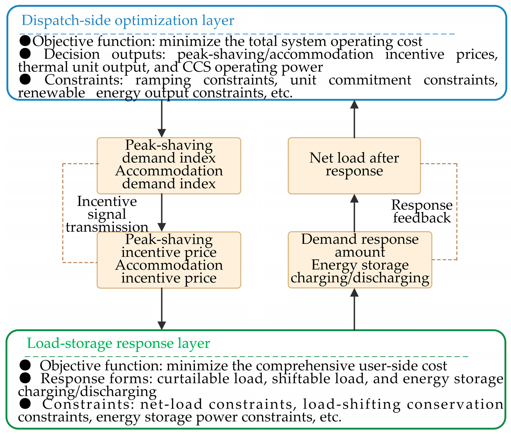
Within the proposed alternating coordination framework, incentive prices transmit low-carbon dispatch requirements from the dispatch side to the load-storage side, while net-load feedback returns the load reconstruction results to the dispatch side after each iteration. This bidirectional information exchange forms the closed-loop interaction shown in Figure 1 and supports iterative coordination. Unlike conventional dispatch models that treat demand response as a fixed input or use static incentive prices, the proposed framework updates incentive signals according to realized response performance and iterative net-load changes.

To prevent incentive prices from increasing monotonically when the demand indices are non-negative, an updating mechanism based on response-gap negative feedback is introduced. The peak-shaving and accommodation incentive prices are updated as follows:

$${\pi }_t^{\mathrm{red},(k+1)}=\mathrm{clip}\left[{\pi }_t^{\mathrm{red},k}+{\kappa }_1\left(D_t^{\mathrm{red},\left(k\right)}-D{R}_t^{\mathrm{red},\left(k\right)}\right)-{\theta }_1\left({\pi }_t^{\mathrm{red},k}-{\pi }_t^{\mathrm{red},0}\right)\right]$$

(48)

$${\pi }_t^{\mathrm{inc},(k+1)}=\mathrm{clip}\left[{\pi }_t^{\mathrm{inc},k}+{\kappa }_2\left(D_t^{\mathrm{inc},\left(k\right)}-D{R}_t^{\mathrm{inc},\left(k\right)}\right)-{\theta }_2\left({\pi }_t^{\mathrm{inc},k}-{\pi }_t^{\mathrm{inc},0}\right)\right]$$

(49)

where $D_t^{\mathrm{red}}$ and $D_t^{\mathrm{inc}}$ represent the peak-shaving response demand and accommodation response demand expected by the dispatch side from the load-storage side at time period t, respectively. ${\kappa }_1$ and ${\kappa }_2$ are the price feedback step sizes, ${\theta }_1$ and ${\theta }_2$ are the price damping coefficients. In the price update, the clip operator confines the incentive prices within the prescribed economic bounds. The lower bound is used to avoid ineffective incentives caused by excessively low prices, whereas the upper bound is used to control user-side incentive payments and prevent excessive price amplification during the iterative update. The response-gap term provides a negative-feedback correction. When the realized load-storage response is lower than the dispatch-side expected response, the incentive price is increased to encourage additional participation. When the realized response reaches or exceeds the expected response, the incentive price is stabilized or reduced to avoid excessive response and unnecessary incentive expenditure. Therefore, the price update acts as a coordination signal rather than a market-clearing price.

The proposed price update can be interpreted as a damped fixed-point iteration for the coupled price-response mapping. Stable iterative behavior is favored when the load-storage response is monotone and bounded with respect to incentive prices and when the feedback gains remain moderate in practical operation. The damping coefficients suppress oscillatory price trajectories, while the relaxation coefficient smooths the updated net load between successive iterations. If a price bound remains active for several iterations, the iteration approaches a boundary fixed point under the corresponding price cap rather than an unconstrained equilibrium.

4. Two-Layer Alternating Solution Method

The dispatch-side layer determines thermal generation, renewable energy accommodation, CCS operation, and carbon-trading decisions using the current net-load profile. The load-storage response layer then optimizes demand response and energy storage operation under the incentive prices issued by the dispatch side. These two layers are coupled through incentive-price transmission and net-load feedback. To solve this coupled source-load-storage dispatch problem, the proposed framework adopts a decomposition-coordination alternating iterative method rather than a strict bi-level/Stackelberg formulation. The lower-layer weighted-sum objective is used only to scalarize the multi-objective response problem. Convergence is defined as stabilization of the iterates and is judged by whether both the average net-load error and the relative objective-function error in Equation (55) fall below the prescribed thresholds. This corresponds to an approximate fixed point of the coupled price-response mapping.

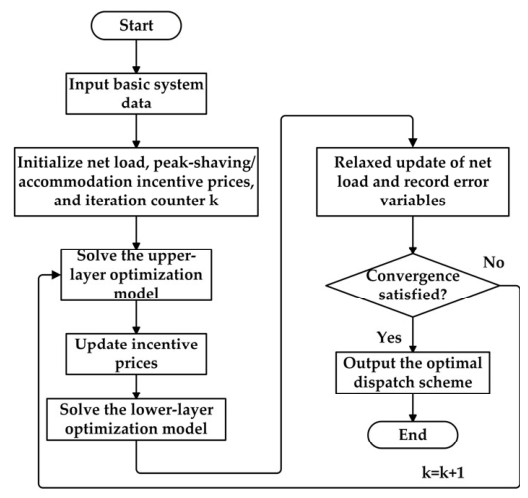
The upper- and lower-layer models are implemented in MATLAB R2022a using YALMIP, and all optimization subproblems are solved by CPLEX. The overall workflow of the proposed two-layer decomposition-coordination alternating iterative solution method is illustrated in Figure 2. Let $K^{\max }=30$ denote the maximum number of iterations. The detailed algorithmic steps are as follows.

(1)

Input the basic system data, including wind/PV forecasts, load curve, thermal-unit parameters, CCS parameters, energy-storage parameters, demand-response parameters, and carbon-market parameters.

(2)

Set the iteration counter to (k = 0). Use the base load as the initial net load, initialize the peak-shaving and accommodation incentive prices, and set the initial actual responses to zero.

(3)

In iteration k, solve the dispatch-side optimization problem using the current net load $L_t^{\mathrm{net},\left(k\right)}$ and obtain the dispatch state required for demand-index calculation and price updating.

(4)

Calculate the peak-shaving and accommodation demand indices according to the dispatch-side operating state. Then obtain the expected response demands and update the two incentive prices using the response-gap negative-feedback rule and the actual response from the previous iteration.

(5)

Input the updated dual incentive prices into the load-storage response layer. The load-storage response problem is solved by the normalized weighted-sum method, and the response amounts and reconstructed net load are obtained.

Specifically, since the response-cost term $F_1$ and the net-load-fluctuation term $F_2$ have different dimensions, payoff-based normalization is applied before scalarization. In each iteration, the payoff bounds of the two terms are obtained by separately minimizing $F_1$ and $F_2$ under the same lower-layer constraints. The normalized component is calculated as follows:

$$F_{m,N}={\displaystyle \frac{(F_m-F_{m,\min })}{(F_{m,\max }-F_{m,\min })}}, m=\mathrm{1,2}$$

(50)

A small positive safeguard is used when the denominator is nearly zero. The scalar lower-layer objective is written as follows:

$$F_L={\chi }_1{F}_{1,N}+{\chi }_2{F}_{2,N}$$

(51)

where the two weights satisfy

$${\chi }_1\ge 0, {\chi }_2\ge 0, {\chi }_1+{\chi }_2=1$$

(52)

The benchmark case adopts ${\chi }_1$ = ${\chi }_2$ = 0.5 so that the load-storage side gives equal preference to the response-cost term and the net-load-fluctuation term.

$$L_t^{\mathrm{net},\mathrm{resp},(k+1)}=L_t^0+L_t^{\mathrm{shift},\mathrm{in},(k+1)}-L_t^{\mathrm{shift},\mathrm{out},(k+1)}-L_t^{\mathrm{cut},(k+1)}+P_t^{\mathrm{ch},(k+1)}-P_t^{\mathrm{dis},(k+1)}$$

(53)

(6)

To suppress oscillations in the interaction variables, a relaxation strategy is used to update the net load:

$$L_t^{\mathrm{net},(k+1)}=\lambda L_t^{\mathrm{net},\mathrm{resp},(k+1)}+(1-\lambda )L_t^{\mathrm{net},\left(k\right)}$$

(54)

where $\lambda \in \left(\mathrm{0,1}\right)$. A larger value of λ assigns greater weight to the current load-storage response, whereas a smaller value produces a smoother updating process.

(7)

After each iteration, convergence is evaluated using the average net-load error and the relative objective-function error:

$$\{\begin{array}{c}{\epsilon }_{L,MAE}^{\left(k\right)}={\displaystyle \frac{1}{T}}{\displaystyle \sum _{t=1}^T}\left|L_t^{\mathrm{net},(k+1)}-L_t^{\mathrm{net},\left(k\right)}\right|\le {\epsilon }_L\hfill \\ {\epsilon }_F^{\left(k\right)}=\left|{\displaystyle \frac{F_U^{(k+1)}-F_U^{\left(k\right)}}{F_U^{\left(k\right)}}}\right|\le {\epsilon }_F\hfill \end{array}$$

(55)

where ${\epsilon }_L$ and ${\epsilon }_F$ are the corresponding convergence thresholds. If both criteria are satisfied, the algorithm stops; otherwise, set (k = k + 1) and return to Step 3.

From the computational perspective, each outer iteration solves one dispatch-side optimization subproblem and one load-storage response subproblem in sequence. When payoff-based normalization is used in the lower layer, two additional auxiliary lower-layer optimizations are solved to obtain the required normalization bounds.

(8)

If the convergence conditions are satisfied, the final dispatch results are output.

For clarity, the key time-series variables involved in the iterative coordination process are summarized in Appendix A (

Table A1. Symbol Table of Key Time-Series Variables.

Symbol	Meaning
$L_t^0$	Base load at time period t
$L_t^{\mathrm{net},\left(k\right)}$	Net load used by the dispatch-side layer in iteration k
$L_t^{\mathrm{net},\mathrm{resp},\left(k\right)}$	Reconstructed net load from the load-storage response layer
$D_t^{\mathrm{red}},D{R}_t^{\mathrm{red}}$	Expected and actual peak-shaving response demand
$D_t^{\mathrm{inc}},D{R}_t^{\mathrm{inc}}$	Expected and actual renewable accommodation response demand
$L_t^{\mathrm{shift},\mathrm{in}},L_t^{\mathrm{shift},\mathrm{out}},L_t^{\mathrm{cut}}$	Shift-in, shift-out, and curtailable load
$P_t^{\mathrm{ch}},P_t^{\mathrm{dis}}$	Energy storage charging and discharging power
${\chi }_1,{\chi }_2,{\kappa }_1,{\kappa }_2,{\theta }_1,{\theta }_2,\lambda$	Preference weights, feedback gains, damping coefficients, and relaxation coefficient

).

5. Case Study

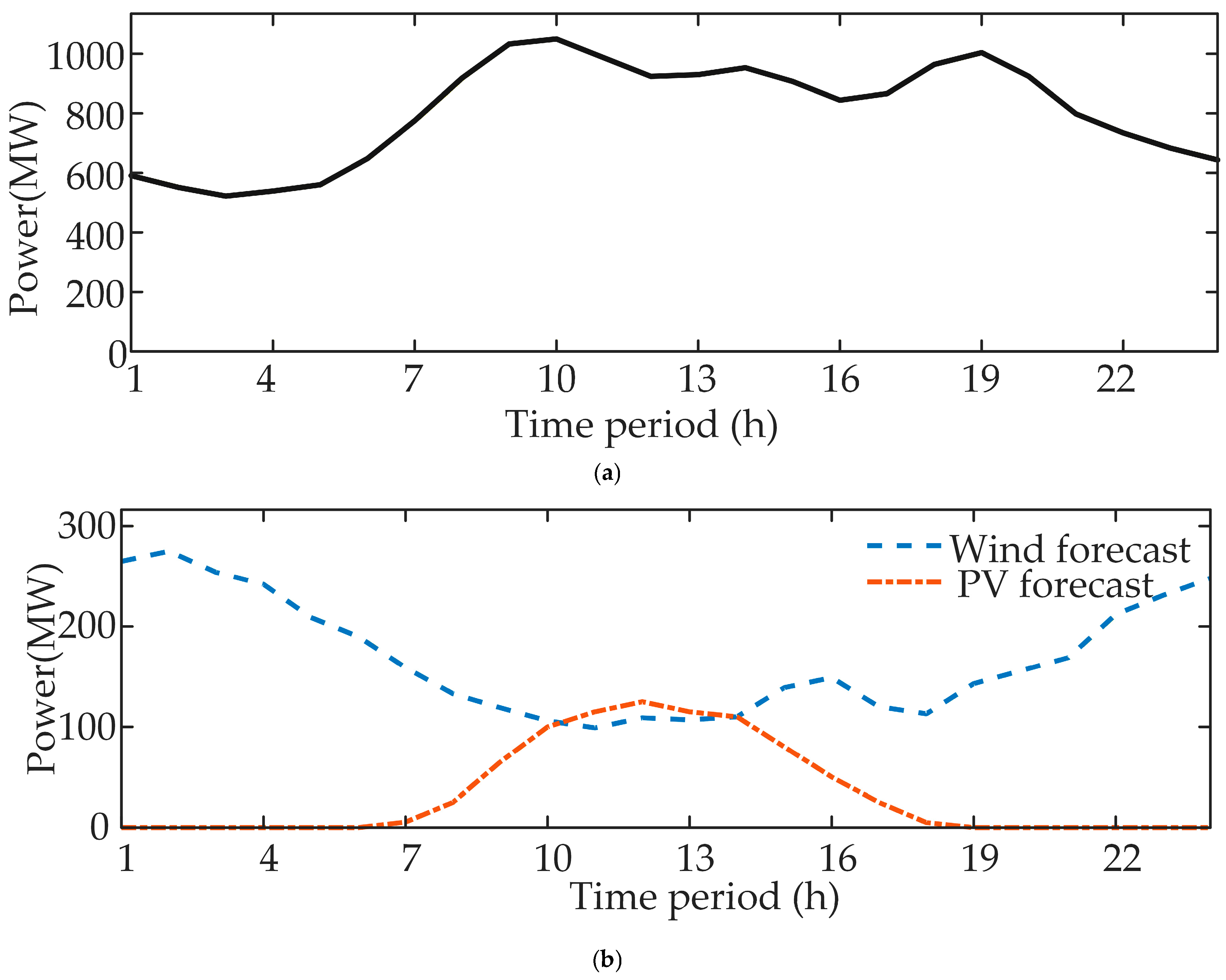
To verify the effectiveness of the proposed upper- and lower-layer alternating coordinated low-carbon economic dispatch method, a typical-day wind–PV–thermal–storage system incorporating demand response and CCS is selected as the case study for simulation analysis. The system includes thermal power units, a wind farm, a photovoltaic power station, a lithium iron phosphate energy storage system, user-side demand response resources, and CCS devices installed on some thermal power units. The dispatch period is 24 h, and the dispatch time interval is denoted by $\Delta t$ and is set to 1 h in the case study. Therefore, power variables in MW are converted into energy quantities in MWh by multiplying by $\Delta t$. All monetary results are reported in CNY; electricity prices and power-related cost coefficients are given in CNY/MWh, while carbon-related cost coefficients are given in CNY/t. To ensure the reproducibility of the case study, the main parameters used in the simulation are summarized in

Table 1. Parameters of thermal power units.

Unit	Pmax (MW)	Pmin (MW)	Ramp Limit (MW/h)	ai	bi	ci	Carbon Emission Coefficient (t/MWh)
G1	460	230	184	0.0211	21.05	1313.60	0.90
G2	300	150	120.0	0.0700	23.90	471.00	0.94
G3	240	120	96	0.0790	21.62	480.29	0.99
G4	120	60	48	0.0480	23.23	639.40	1.05
G5	130	65	52	0.0630	16.51	502.70	1.05

,

Table 2. Parameters of CCS, carbon trading, and renewable energy curtailment.

Parameter	Symbol	Value	Unit
Fixed operating power of CCS	Piccs,fix	15	MW
Unit energy consumption for carbon capture	γE	0.269	MWh/t
Maximum operating power of CCS	Piccs,max	170	MW
Maximum capture efficiency	ζimax	90	%
Ramp limit of CCS	Riccs	65	MW/h
Unit CO2 storage cost	cstore	50	CNY/t
Base carbon price	μ0	100	CNY/t
Carbon price growth coefficient	ω	0.25	—
Wind curtailment penalty	gw	180	CNY/MWh
PV curtailment penalty	gs	180	CNY/MWh

,

Table 3. Parameters of the energy storage system.

Parameter	Symbol	Value	Unit
Rated capacity of energy storage	Ecap	230	MWh
Maximum charging power	PESch,max	75	MW
Maximum discharging power	PESdis,max	75	MW
Upper limit of SOC	SOCmax	0.90	—
Lower limit of SOC	SOCmin	0.10	—
Initial SOC	SOC0	0.50	—
Charging efficiency	ηch	0.9	—
Discharging efficiency	ηdis	0.9	—
Equivalent energy storage degradation cost coefficient [30]	cdeg	50	CNY/MWh

and

Table 4. Algorithmic and carbon-market parameters.

Variable	Value	Unit
$L_t^{\mathrm{cut},\max }$	157.5	MW
$L_t^{\mathrm{shift},\mathrm{out},\max }$, $L_t^{\mathrm{shift},\mathrm{in},\max }$	210	MW
${\lambda }_t^{\mathrm{buy}}$	350 (t = 1–6); 650 (t = 7, 16–17, 22–24); 950 (t = 8–15, 18–21)	CNY/MWh
${\pi }^{\mathrm{red},\left(0\right)}$	55	CNY/MWh
${\pi }^{\mathrm{inc},\left(0\right)}$	65	CNY/MWh
${\pi }_{\min }^{\mathrm{red}}$	27	CNY/MWh
${\pi }_{\max }^{\mathrm{red}}$	113	CNY/MWh
${\pi }_{\min }^{\mathrm{inc}}$	29	CNY/MWh
${\pi }_{\max }^{\mathrm{inc}}$	180	CNY/MWh
${\epsilon }_L$	10.5	MW
${\epsilon }_F$	1.0 × 10−2	—
$\lambda$	0.95	—
$K$	4	—
$L_k$	200, 400, 600, 800	t
${\Omega }_{CCS}$	{G1, G2, G3}	—

. Specifically, Table 1 presents the operating and cost parameters of the thermal power units; Table 2 lists the parameters related to CCS, carbon trading, and renewable energy curtailment; Table 3 presents the parameters of the lithium iron phosphate energy storage system; and Table 4 summarizes the algorithmic, incentive-price, and additional carbon-market parameters. The detailed time-series input profiles used in the case study are provided in Appendix B, as shown in Figure A1.

5.1. Scenario Settings

To progressively evaluate the effects of source-side low-carbon measures, energy storage, demand response, and the proposed response-gap feedback mechanism, six comparison scenarios are established as follows. The scenarios are designed in a stepwise manner so that the marginal contribution of each resource or mechanism can be identified. In particular, Scenarios 5 and 6 are used to compare the effect of introducing the actual response-deviation correction term into the dynamic incentive price update.

Scenario 1: A benchmark scenario in which only thermal power, wind power, and photovoltaic generation participate in dispatch.

Scenario 2: A low-carbon dispatch scenario with ladder-type carbon trading and CCS integrated on the source side.

Scenario 3: A low-carbon and energy-storage coordinated scenario with an energy storage system.

Scenario 4: A source-load-storage coordinated scenario considering static-incentive one-shot demand response.

Scenario 5: A comparison scenario using a dynamic incentive price-updating mechanism without negative feedback, in which prices are adjusted according to demand indices without considering actual response deviations.

Scenario 6: A source-load-storage coordinated low-carbon dispatch scenario using the proposed response-gap negative-feedback dynamic incentive price-updating mechanism, in which incentive prices are corrected according to deviations between expected and actual load-storage responses.

5.2. Comparative Analysis of Economy and Low-Carbon Performance Under Different Scenarios

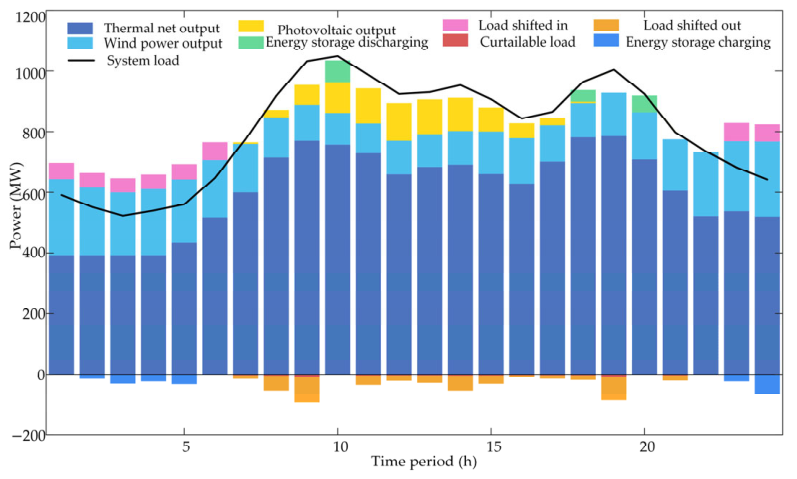
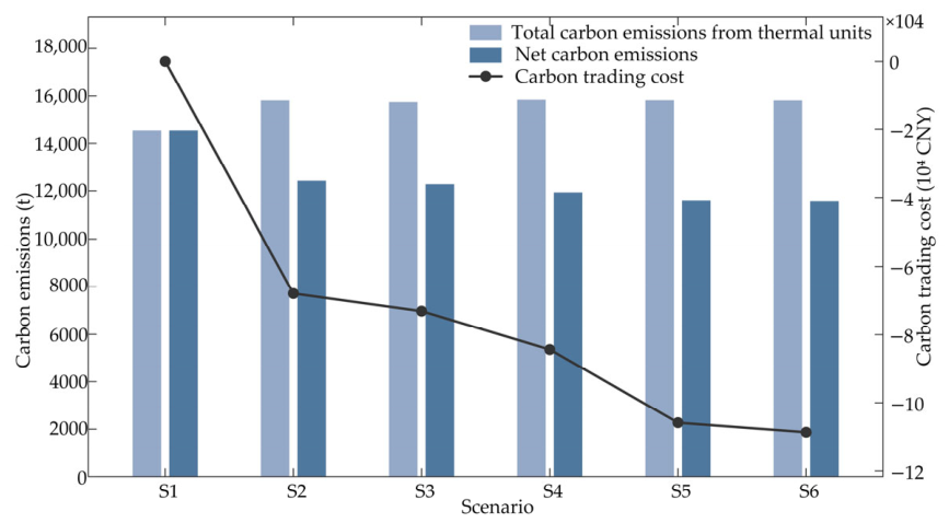
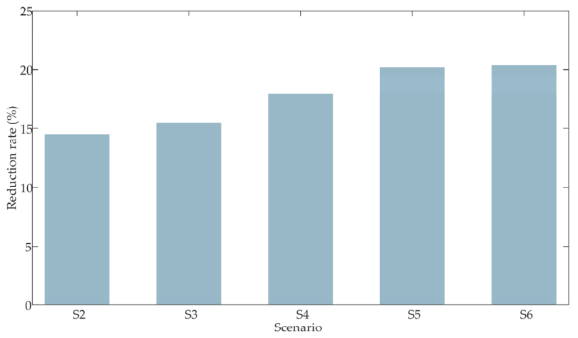
The results are presented in

Table 5. Comparison of dispatch-side operating cost components among different scenarios.

Scenario	1	2	3	4	5	6
Fuel cost (CNY)	545,999	606,702	601,224	566,175	565,030	564,374
Ramp cost (CNY)	30,350	30,317	25,638	35,004	26,145	24,141
Wind and PV curtailment penalty cost (CNY)	213,300	100,775	79,986	41,989	25,244	24,441
Demand response incentive cost (CNY)	0	0	0	47,976	45,219	32,766
Energy storage degradation cost (CNY)	0	0	24,480	18,012	18,220	17,863
CO2 storage cost (CNY)	0	169,530	173,136	195,423	210,915	211,914
Carbon trading cost (CNY)	0	−67,880	−73,064	−84,349	−105,836	−108,645
Dispatch-side operating cost (CNY)	789,649	839,444	831,400	820,230	784,937	766,854

and Figure 3, Figure 4 and Figure 5. Table 5 compares the major cost components and dispatch-side operating costs across the six scenarios; Figure 3 illustrates the hourly power balance under Scenario 6; and Figure 4 and Figure 5 compare total and net carbon emissions, carbon-trading costs, and net carbon-emission reduction rates across the different scenarios. It should be emphasized that Scenarios 5 and 6 are designed to compare the marginal effect of the response-gap negative-feedback mechanism, and the main difference between them lies in whether the actual response-deviation correction term is introduced into the incentive-price update.

As shown in Table 5, the progression from Scenario 1 to Scenario 6 indicates that the advantage of the proposed framework does not come from a single technology, but from coordinated flexibility on the source, load, and storage sides. When low-carbon coordination and flexible resources are absent, the system relies mainly on thermal generation, so emission-control measures cannot be effectively translated into operating savings. After CCS and ladder-type carbon trading are introduced, net emissions are reduced, but the additional capture burden also increases source-side operating cost, which suggests that emission reduction alone does not necessarily lower total cost. Energy storage then plays a buffering role by absorbing surplus renewable generation and alleviating thermal ramping pressure, thereby improving temporal supply-demand matching and reducing curtailment. With the further introduction of demand response, part of the peak load is shifted away from high-cost periods, which helps reduce fuel consumption and system adjustment burden.

The key improvement appears when the incentive mechanism is updated through response-gap negative feedback. Compared with static or conventional dynamic incentives, the proposed mechanism aligns price signals more closely with realized response behavior, avoiding persistent over-incentivization when the response has already been sufficient and strengthening incentives when the response is inadequate. In this sense, the price update acts as a closed-loop coordination signal rather than a purely exogenous incentive. As a result, the system achieves more balanced coordination among CCS, storage, and demand response, while reducing ramping stress, renewable curtailment, and incentive expenditure.

From a practical perspective, these results indicate that low-carbon dispatch in high-renewable systems should be treated as a coordinated control problem rather than a sequence of isolated technologies. CCS suppresses emissions, storage smooths intra-day imbalance, and demand response reshapes load on the user side. The proposed response-gap negative-feedback mechanism links these resources through iterative price correction, making the dispatch process more stable and less prone to inefficient incentive escalation. This is particularly relevant for systems with strong renewable variability, where the objective is not only to reduce emissions, but also to maintain economically acceptable operation under limited flexibility.

5.3. Analysis of Renewable Energy Accommodation Under Different Scenarios

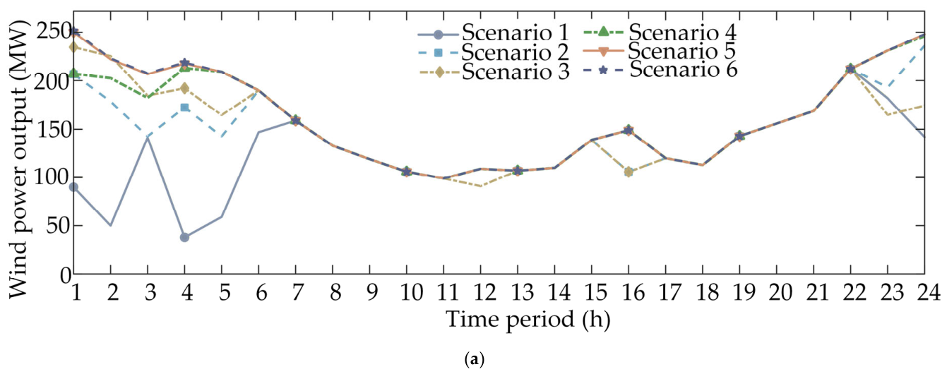
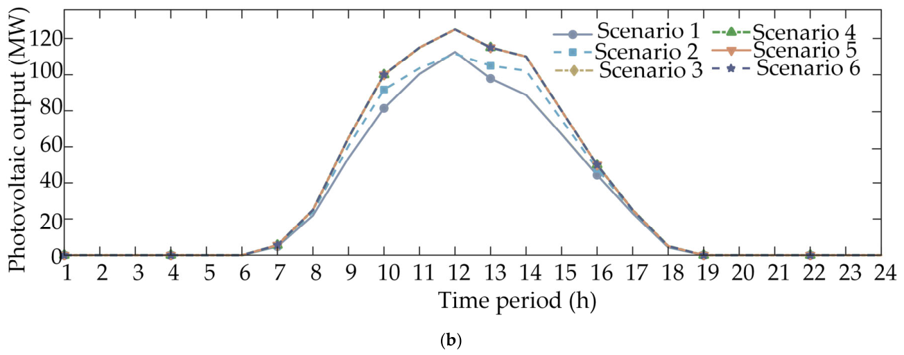
To further analyze the effects of different resource configurations and dispatch mechanisms on renewable energy accommodation, the actual wind and photovoltaic outputs across scenarios are compared, as shown in Figure 6. Specifically, Figure 6a shows wind power output, while Figure 6b shows photovoltaic output. The closer the actual wind and photovoltaic outputs are to the forecast available outputs, the smaller the renewable energy curtailment and the stronger the system accommodation capability.

As shown in Figure 6, the renewable accommodation level improves progressively as additional flexibility resources are introduced into the system. In the benchmark case, the limited flexibility of the source side makes it difficult to absorb renewable fluctuations during low-load and high-output periods, so wind and photovoltaic curtailment remains noticeable. After CCS and ladder-type carbon trading are introduced, thermal generation is more strongly constrained by carbon costs, which creates additional room for renewable energy accommodation. When energy storage is further added, surplus renewable output can be absorbed during peak generation periods and released later, thereby improving temporal balance and reducing curtailment. The introduction of demand response further enhances this effect by reshaping the load profile and increasing source-load matching capability.

The proposed response-gap negative-feedback pricing mechanism provides an additional improvement in coordination quality. By adjusting incentive prices according to the deviation between expected and realized responses, the dispatch side can avoid persistent over-incentivization while still maintaining sufficient regulation when the actual response is inadequate. As a result, both wind and photovoltaic outputs remain closer to their available levels across most periods, indicating more effective renewable accommodation. From a practical perspective, this shows that renewable integration in low-carbon dispatch should rely not only on emission constraints, but also on coordinated flexibility from storage and demand response, with closed-loop pricing used to align the realized response with dispatch requirements. Overall, the renewable accommodation rate in Scenario 6 is about 21.5 percentage points higher than that in Scenario 1.

5.4. Analysis of Peak-Shaving and Valley-Filling Effects of Net Load Under Different Scenarios

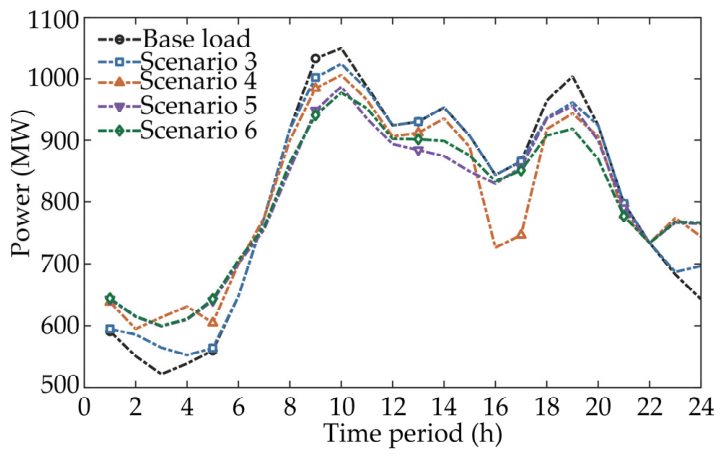
To analyze the regulation effects of energy storage and demand response on the system load curve, the original load and the net-load curves in Scenarios 3–6 are compared, as shown in Figure 7.

As shown in Figure 7, the original load curve exhibits distinct morning and evening peaks and a low-load valley in the early morning, which leads to a pronounced peak-valley difference. After energy storage is introduced, charging during valley periods and discharging during peak periods partially smooth the net-load profile. With the further participation of demand response, part of the flexible load is shifted away from peak periods or adjusted according to system regulation needs, thereby enhancing the peak-shaving and valley-filling effects.

The difference between Scenarios 5 and 6 further illustrates the role of response-gap correction. In Scenario 5, dynamic incentives can guide load-storage regulation, but the price signal is updated mainly according to system regulation demand, without directly correcting the mismatch between expected and realized responses. Therefore, local over-response or insufficient response may still occur. In Scenario 6, the response-gap negative-feedback mechanism adjusts incentive prices according to actual response performance, strengthening the signal when the response is insufficient and weakening it when the response is adequate. This closed-loop correction improves the temporal matching between dispatch-side regulation demand and load-storage-side response, resulting in a smoother net-load curve and more coordinated peak-valley regulation.

5.5. Analysis of Coordinated Regulation Effects of Energy Storage and Demand Response

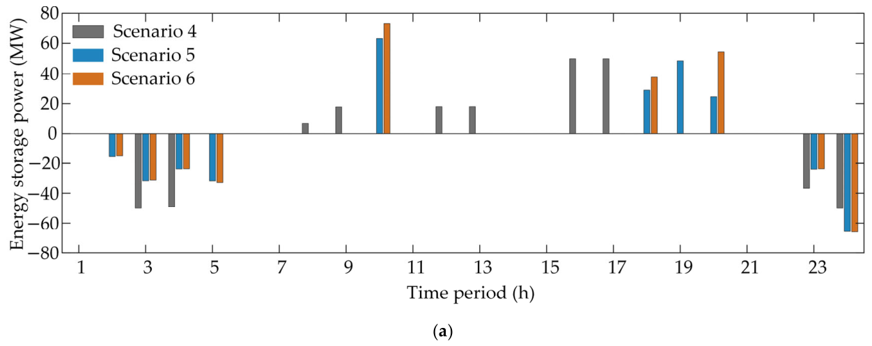
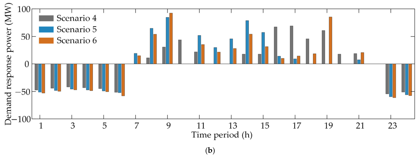
To further analyze the roles of energy storage and demand response in source-load-storage coordinated dispatch, Figure 8 compares the energy storage charging/discharging power and demand response power in Scenarios 4–6. Figure 8a shows the energy storage charging/discharging behavior, and Figure 8b shows the comprehensive regulation power of demand response.

As shown in Figure 8a, the storage operation patterns differ noticeably among Scenarios 4–6. Under static incentives, charging and discharging are relatively scattered, indicating weak alignment with time-varying system regulation needs. Under dynamic incentives, storage operation becomes more regular: charging mainly occurs during valley-load or renewable-surplus periods, while discharging occurs during high-load periods. This pattern improves temporal flexibility and supports net-load smoothing.

The comparison between Scenarios 5 and 6 shows the additional effect of response-gap correction. In Scenario 5, dynamic pricing increases response intensity, but some regulation remains excessive or poorly timed. In Scenario 6, the feedback term guides storage and demand response toward periods with stronger peak-shaving or renewable accommodation needs. Storage provides short-term energy shifting, while demand response reshapes the user-side load profile. Their complementarity reduces ineffective response and improves load-storage regulation efficiency.

5.6. Analysis of Dynamic Regulation Characteristics of Incentive Prices

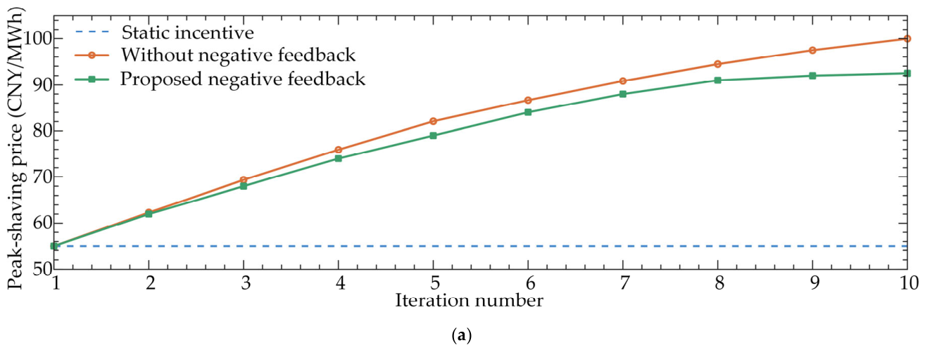
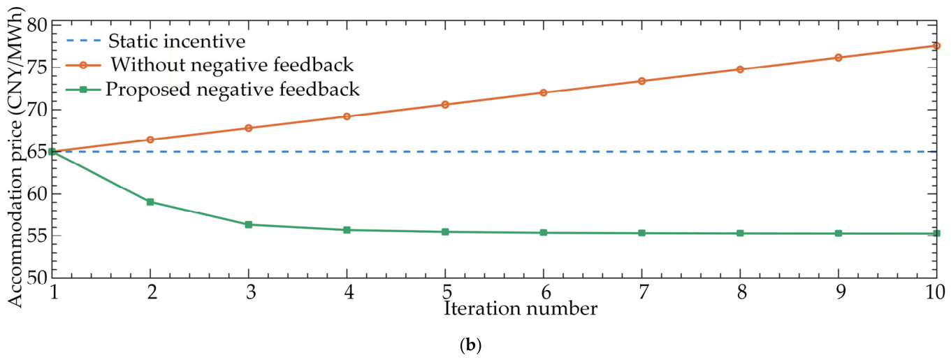
To compare the price regulation characteristics of different incentive mechanisms, Figure 9 presents the trajectories of peak-shaving and accommodation incentive prices under static incentives, dynamic incentives without negative feedback, and the proposed negative-feedback dynamic incentives. Specifically, Figure 9a shows the peak-shaving incentive price trajectory, while Figure 9b shows the accommodation incentive price trajectory.

As shown in Figure 9, the three incentive mechanisms show different price-evolution patterns. The static incentive remains fixed during the iteration process and therefore acts only as a one-shot price signal, with limited adaptability to time-varying regulation needs. The dynamic incentive without negative feedback can reflect changes in the demand indices, but its price continues to increase because the update does not consider response completion. This may cause excessive incentive expenditure when the actual response is already sufficient.

By contrast, the proposed response-gap negative-feedback mechanism adjusts both the direction and magnitude of price changes according to realized response performance. The peak-shaving incentive increases when the response is insufficient, but its growth weakens as the response gap narrows. The renewable accommodation incentive decreases and then stabilizes once the accommodation response satisfies the system requirement. These trajectories show that the proposed mechanism preserves the adaptability of dynamic pricing while avoiding continuous price escalation, thereby improving response matching and incentive cost-effectiveness.

5.7. Step-Size Sensitivity Analysis

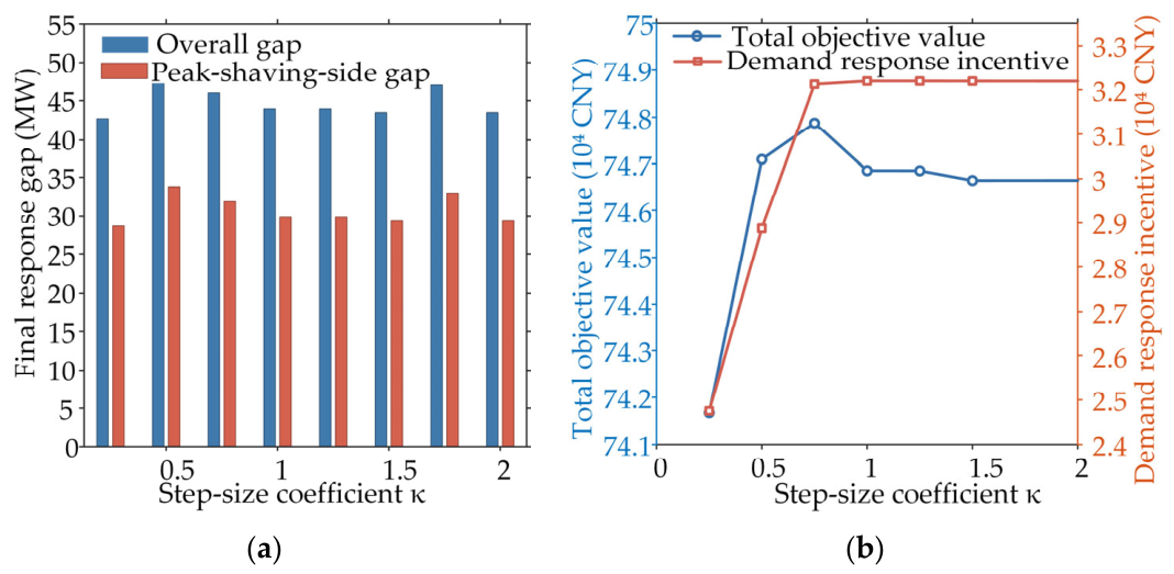
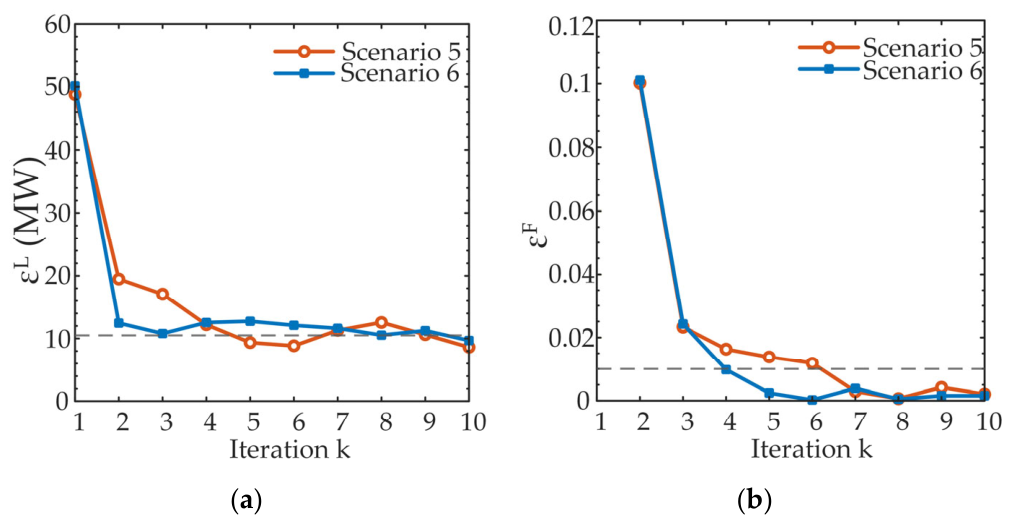
To analyze the effect of the price-updating step size on negative-feedback regulation, Figure 10 presents the final response-matching degree and economic indicators under different step-size coefficients. Figure 10a compares the final-iteration response gaps, while Figure 10b shows the dispatch-side operating cost and demand response incentive cost. To further verify the iterative stability of the proposed mechanism, Figure 11 compares the convergence trajectories of Scenarios 5 and 6 using the average net-load error and the relative objective-function error.

As shown in Figure 10, the price feedback step size affects both response correction and operating economy. When the step size is small, incentive prices change slowly, so the response gap cannot be corrected effectively and the load-storage response may lag behind dispatch-side regulation demand. As the step size increases, price signals become more effective in guiding response adjustment, and the response gap decreases. However, after the step size reaches a moderate range, the improvement in response matching becomes limited, indicating that the regulation effect gradually approaches saturation.

The economic indicators reveal the corresponding tradeoff. A larger step size strengthens the incentive signal, but it also increases DR incentive expenditure and may amplify price fluctuations. Therefore, the step size should not be selected only to minimize the response gap; it should balance response matching, incentive cost, and price smoothness. The benchmark setting used in this study provides such a practical compromise and supports stable iterative behavior under the tested parameter settings.

For practical implementation, ${\kappa }_1$ and ${\kappa }_2$ should be selected to balance response correction and price smoothness. Excessively small gains lead to sluggish price adjustment and slow response matching, whereas excessively large gains may cause overshooting, oscillation, and repeated activation of the clipping bounds. In the case study, ${\kappa }_1$ = 0.24, ${\kappa }_2$ = 0.45, ${\theta }_1$ = 0.10, and ${\theta }_2$ = 0.55 produced bounded and stable price trajectories; larger gains increased price swings and incentive expenditure without proportional improvement in response matching. Therefore, the convergence reported in this paper is interpreted as stabilization of the iterates to an approximate fixed point of the coupled price-response mapping.

As shown in Figure 11a, the average net-load errors of both scenarios decrease rapidly in the early iterations and fall below the prescribed threshold, indicating that the net-load feedback process becomes stable. Compared with Scenario 5, Scenario 6 maintains a lower final net-load error, which shows that the response-gap negative-feedback mechanism improves the matching between the dispatch-side expected response and the load-storage-side actual response. Figure 11b further shows that the relative objective-function errors of both scenarios also decrease to below the convergence threshold. The final objective-function error in Scenario 6 is lower than that in Scenario 5, indicating that the proposed mechanism can suppress ineffective price correction and improve the observed stability of the alternating coordination process. Therefore, Figure 11 provides empirical stability evidence for the proposed price-response iteration under the tested case-study settings, rather than a theoretical guarantee of global convergence under all possible parameter settings.

5.8. Weight Sensitivity of the Lower-Layer Objective

To test whether the dispatch performance depends strongly on the lower-layer objective preference, five representative weight pairs were selected for the normalized weighted-sum objective: (0.2, 0.8), (0.4, 0.6), (0.5, 0.5), (0.6, 0.4), and (0.8, 0.2). In each pair, the first value is ${\chi }_1$, corresponding to the response-cost term $F_1$, and the second value is ${\chi }_2$, corresponding to the net-load-fluctuation term $F_2$. The equal-weight pair is the default preference setting and is used as the benchmark for the sensitivity comparison.

Table 6. Sensitivity analysis of lower-layer objective weights.

Weights (${\mathit{\chi }}_1$, ${\mathit{\chi }}_2$)	Obj. (CNY)	Cost Red. (%)	CO2 Red. (%)	RE Acc. Increase (%)
(0.2, 0.8)	788,254	0.18	19.5	18.0
(0.4, 0.6)	769,989	2.49	19.9	19.3
(0.5, 0.5)	766,854	2.89	20.4	21.5
(0.6, 0.4)	758,798	3.91	20.2	20.2
(0.8, 0.2)	744,208	5.57	20.5	21.3

shows the expected tradeoff between the two lower-layer preferences. Increasing ${\chi }_1$ places more emphasis on the response-cost term and reduces the dispatch objective from 788,254 CNY to 744,208 CNY, while the cost-reduction rate increases from 0.18% to 5.75%. Across all tested weights, net CO₂ emissions remain within 11,563–11,699 t, the CO₂ reduction rate remains within 19.5–20.5%, and the renewable energy accommodation improvement remains within 18.0–21.5 percentage points. These results indicate that the main economic, emission-reduction, and renewable-accommodation benefits are robust to reasonable changes in the lower-layer objective weights.

5.9. Robustness Test Under Demand Response Uncertainty

To further examine the robustness of the proposed closed-loop feedback mechanism, a Monte Carlo experiment is conducted by introducing uncertainty into the realized demand response. In practice, the actual response may deviate from the scheduled value due to user behavior and execution errors. Accordingly, the response factor is assumed to follow a uniform distribution, i.e., ${\xi }_{t,s}\sim U\left(0.9, 1.1\right)$, where $s$ denotes the Monte Carlo sample and ${\xi }_{t,s}$ indicates a ±10% variation around the scheduled demand response. A total of 100 Monte Carlo samples are generated, and the same uncertainty realizations are applied to Scenarios 5 and 6 to ensure a fair comparison.

Table 7. Relative performance improvement of Scenario 6 over Scenario 5 under ±10% demand-response uncertainty.

Metric	Improvement of Scenario 6 over Scenario 5
Mean dispatch-side operating cost reduction	3.90%
DR incentive cost reduction	28.45%
Net CO2 emissions reduction	0.23%
Net-load fluctuation reduction	2.81%
Renewable accommodation improvement	0.091%

summarizes the relative performance improvement of Scenario 6 over Scenario 5 under demand-response uncertainty.

Table 7 shows that Scenario 6 maintains better performance than Scenario 5 under ±10% demand-response uncertainty. The mean dispatch-side operating cost is reduced by 3.90%, and the DR incentive cost is reduced by 28.45%, indicating that the proposed feedback pricing mechanism still maintains clear economic advantages when the realized response deviates from the scheduled value. Meanwhile, the net-load fluctuation is reduced by 2.81%, and the renewable accommodation performance is slightly improved, suggesting that the closed-loop scheme also preserves its operational effectiveness under uncertainty. Although the reduction in net CO₂ emissions is relatively limited, the overall results confirm that the proposed method is resilient to moderate response uncertainty.

6. Discussion

The results extend previous studies showing that coordinated demand response and energy storage can reduce operating costs, carbon emissions, and net-load fluctuations [12,13,14]. This study further indicates that coordination performance depends not only on the availability of flexible resources but also on the updating logic of incentive prices. Compared with recent bi-level dispatch and incentive-based coordination methods [23,24,25,26,27], the proposed framework differs mainly in the response-gap feedback design. Existing methods usually transmit price or demand signals to guide user-side resources, whereas the proposed method further compares the dispatch-side expected response with the realized load-storage response and uses this deviation to correct incentive prices. In this sense, Scenario 5 represents a dynamic incentive coordination benchmark without response-gap correction, while Scenario 6 adds the proposed feedback term. The comparison between these two scenarios shows that the response-gap mechanism reduces incentive expenditure and net-load fluctuation while maintaining favorable low-carbon and renewable-accommodation performance.

The results also complement source-side studies combining CCS with carbon-trading mechanisms [18,19,20]. In the proposed framework, CCS and ladder-type carbon trading provide source-side emission-reduction signals, while demand response and energy storage reshape the net load. Their coordinated operation therefore improves economic and low-carbon performance more effectively than source-side measures alone. It should be noted that the carbon trading cost is evaluated under an hourly equivalent settlement mechanism with exogenous carbon prices and no inter-period allowance banking. Under this setting, surplus allowances can be sold within each dispatch period, so the reported negative carbon trading cost should be interpreted as trading revenue under the assumed market rule rather than as a market-clearing result.

Although the demand-response uncertainty experiment demonstrates the robustness of the proposed method under moderate response deviations, the current validation is still based on a typical-day test system. Future work will further examine the proposed method under different renewable energy penetration levels and larger-scale power systems to evaluate its generality and scalability.

7. Conclusions

This paper proposes a source-load-storage alternating coordinated low-carbon economic dispatch method based on response-gap negative-feedback dual incentives for power systems with high renewable energy penetration. The main conclusions are as follows.

(1)

The proposed method establishes closed-loop coordination between dispatch-side low-carbon optimization and load-storage-side flexible response through incentive-price transmission and net-load feedback. This coordination improves source-load matching and reduces the dispatch-side operating cost by 2.89% compared with Scenario 1.

(2)

The coordinated operation of energy storage, demand response, CCS, and ladder-type carbon trading improves both economic and low-carbon performance. Energy storage and demand response smooth the net-load curve and promote renewable energy accommodation, while CCS and carbon trading reduce net carbon emissions. In the case study, the net carbon emission reduction reaches 20.4%, and the renewable energy accommodation rate increases by approximately 21.5 percentage points.

(3)

The response-gap negative-feedback pricing mechanism improves the adaptability and cost-effectiveness of incentive regulation. By incorporating the deviation between expected and actual responses, incentive prices increase under insufficient response and stabilize or decrease under adequate response, thereby reducing ineffective incentive expenditure and improving response matching.

(4)

The sensitivity and robustness analyses show that the main benefits of the proposed method are not strongly dependent on the equal-weight lower-layer objective setting and remain effective under moderate demand-response uncertainty. These results indicate that response-gap feedback can support economic, low-carbon, and adaptive source-load-storage coordination in high-renewable power systems.

References

1. Xiao, X.; Zheng, Z. New power systems dominated by renewable energy towards the goal of emission peak & carbon neutrality: Contribution, key techniques, and challenges. Adv. Eng. Sci. 2022, 54, 47–59. (In Chinese) [Google Scholar] [CrossRef]
2. Ghanbarzadeh, T.; Habibi, D.; Aziz, A. Addressing reliability challenges in generation capacity planning under high penetration of renewable energy resources and storage solutions: A review. Renew. Sustain. Energy Rev. 2025, 212, 115461. [Google Scholar] [CrossRef] [Scilit]
3. Zhuo, Z.; Zhang, N.; Xie, X.; Li, H.; Kang, C. Key technologies and development challenges of power systems with high proportion of renewable energy. Autom. Electr. Power Syst. 2021, 45, 171–191. (In Chinese) [Google Scholar] [CrossRef]
4. Yuan, T.; Zhang, W. A review of research on source-storage-load coordinated planning for new power system. Proc. CSEE 2025, 45, 6664–6683. (In Chinese) [Google Scholar] [CrossRef]
5. Yue, X.; Liao, S.; Xu, J.; Ke, D.; Wang, H.; Yang, J.; He, X. Collaborative optimization of renewable energy power systems integrating electrolytic aluminum load regulation and thermal power deep peak shaving. Appl. Energy 2024, 373, 123869. [Google Scholar] [CrossRef] [Scilit]
6. Wei, W.; Jiang, F.; Dai, S.; Chen, C.; Chen, L. Economic optimization of deep peak regulation of thermal power units taking into account the risk of emergency storage on the demand side. Power Syst. Prot. Control 2022, 50, 153–162. (In Chinese) [Google Scholar] [CrossRef]
7. Yin, W.; Li, Y.; Hou, J.; Miao, M.; Hou, Y. Coordinated planning of wind power generation and energy storage with decision-dependent uncertainty induced by spatial correlation. IEEE Syst. J. 2023, 17, 2247–2258. [Google Scholar] [CrossRef] [Scilit]
8. Chu, Y.; Liu, Y.; Liu, Y.; Hou, S. Two-stage wind-storage dispatch strategy considering efficient utilization of energy storage. Electr. Power Eng. Technol. 2026, 45, 95–104. (In Chinese) [Google Scholar] [CrossRef]
9. Lyu, Q.; Li, M.; Wei, W.; Chen, L.; Mei, S. Low-carbon economic dispatch of power systems with energy storage and wind power based on parametric programming. Electr. Power Autom. Equip. 2023, 43, 12–18+43. (In Chinese) [Google Scholar] [CrossRef]
10. Chen, Y.; Wu, C.; Jiao, Y.; Sun, Z.; Dai, S.; Zhang, P. Coordinated optimal operation strategy of thermal power and energy storage considering demand response and energy storage life model. Electr. Power Autom. Equip. 2022, 42, 16–24. (In Chinese) [Google Scholar] [CrossRef]
11. Liang, Z.; Chung, C.Y.; Yin, X.; Fu, X.; Wang, Q.; Zhu, J. Robust energy management of hybrid microgrids via a nonintrusive load monitoring framework with dual-task learning. IEEE Trans. Smart Grid 2026. Epub ahead of printing. [Google Scholar] [CrossRef] [Scilit]
12. Han, H.; Wei, T.; Wu, C.; Xu, X.; Zang, H.; Sun, G.; Wei, Z. A low-carbon dispatch strategy for power systems considering flexible demand response and energy storage. Front. Energy Res. 2022, 10, 883602. [Google Scholar] [CrossRef] [Scilit]
13. Zhang, Y.; Sun, P.; Ji, X.; Yang, M.; Ye, P. Low-carbon economic dispatch of integrated energy systems considering full-process carbon emission tracking and low carbon demand response. IEEE Trans. Netw. Sci. Eng. 2024, 11, 5417–5431. [Google Scholar] [CrossRef] [Scilit]
14. Liu, Z.; Xing, H.; Cheng, H.; Ye, Y. Bi-level optimal scheduling of integrated energy system considering carbon emission flow and demand response. High Volt. Eng. 2023, 49, 169–178. (In Chinese) [Google Scholar] [CrossRef]
15. Li, J.; Dong, F.; Guo, Q.; Yan, J.; Luo, X.; Li, Q.; Zhu, X.; Li, C. Multi-objective low-carbon dispatch of power system with energy storage considering carbon capture equipment and peak regulation initiative. Electr. Power Autom. Equip. 2026, 46, 175–185. (In Chinese) [Google Scholar] [CrossRef]
16. Geng, X.; Zhang, J.; He, Y.; Yan, R.; Lyu, G.; Liu, Y. Low-carbon optimal dispatch of integrated energy system coupled with liquid-storage CCS and ORC. Electr. Power Eng. Technol. 2026, 45, 1–11. (In Chinese) [Google Scholar] [CrossRef]
17. Sun, H.; Zou, H.; Wen, J.; Ke, W.; Kou, L. Optimal scheduling considering carbon capture and demand response under uncertain output scenarios for wind energy. Sustainability 2024, 16, 970. [Google Scholar] [CrossRef] [Scilit]
18. Song, J.; Zhang, Z.; Mu, Y.; Wang, X.; Chen, H.; Pan, Q.; Li, Y. Enhancing environmental sustainability via interval optimization for low-carbon economic dispatch in renewable energy power systems: Leveraging the flexible cooperation of wind energy and carbon capture power plants. J. Clean. Prod. 2024, 442, 140937. [Google Scholar] [CrossRef] [Scilit]
19. Wang, T.; Jin, Y.; Li, Y. Optimization scheduling of carbon capture power systems considering energy storage coordination and dynamic carbon constraints. Processes 2025, 13, 1758. [Google Scholar] [CrossRef] [Scilit]
20. Huang, L.; Zhong, F.; Lai, C.S.; Zhong, B.; Xiao, Q.; Hsu, W. A ladder-type carbon trading-based low-carbon economic dispatch model for integrated energy systems with flexible load and hybrid energy storage optimization. Energies 2025, 18, 3679. [Google Scholar] [CrossRef] [Scilit]
21. Yuan, G.; Liu, P.; Tang, F.; Tian, W. Source-load coordinated optimal dispatch considering green electricity certificate and carbon trading system. Acta Energ. Sol. Sin. 2022, 43, 190–195. (In Chinese) [Google Scholar] [CrossRef]
22. Li, L.; Li, D.; Zhang, Y.; Zhou, S.; Song, J.; Yu, L.; Wang, W.; Wang, Y. Low-carbon economic optimization of park integrated energy system under hybrid market regulation: A multi-scenario dispatch system integrating ladder-type carbon trading and green certificate trading. Expert Syst. Appl. 2026, 297, 129232. [Google Scholar] [CrossRef] [Scilit]
23. Liao, W.; Liu, D.; Wu, Y.; Weng, J. Low-carbon economic dispatch of power system considering source-load uncertainties and users response behavior. Proc. CSEE 2024, 44, 905–918. (In Chinese) [Google Scholar] [CrossRef]
24. Woo, Y.-B.; Moon, I. Bilevel optimization for multi-user systems with mixed demand response programs for enhanced operational efficiency in electric power grids. Appl. Energy 2025, 399, 126507. [Google Scholar] [CrossRef] [Scilit]
25. Meng, Y.; Wang, Y.; Sun, S.; Wang, S.; Zhang, H. Multi-objective optimal dispatching of demand response-enabled microgrid considering uncertainty of renewable energy generations based on two-level iterative strategy. Energy Rep. 2023, 9, 1842–1858. [Google Scholar] [CrossRef] [Scilit]
26. Zhang, H.; Yang, Y.; Zhao, X.; Xu, N.; Li, C.; Xue, W. Bi-level optimal dispatch strategy for regional integrated energy system considering demand response. Electr. Power 2021, 54, 141–150. (In Chinese) [Google Scholar] [CrossRef]
27. Zhao, X.; Liang, Y.; Sun, M.; Mao, Y. Convex relaxation and bi-level iterative algorithm for dynamic optimal dispatch model of AGC units. Autom. Electr. Power Syst. 2022, 46, 228–238. (In Chinese) [Google Scholar] [CrossRef]
28. Cui, Y.; Gu, C.; Fu, X.; Deng, G.; Zhao, Y.; Tang, Y. Low-carbon economic dispatch of integrated energy system with carbon capture power plants considering generalized electric heating demand response. Proc. CSEE 2022, 42, 8431–8446. (In Chinese) [Google Scholar] [CrossRef]
29. Ministry of Ecology and Environment of the People’s Republic of China. Total Allowance and Allocation Plan for the National Carbon Emissions Trading Power Generation Industry in 2023 and 2024. Available online: https://www.mee.gov.cn/xxgk2018/xxgk/xxgk06/202407/t20240702_1080579.html (accessed on 12 July 2026). (In Chinese)
30. Yin, H.; Lu, X.; Zhou, K. Load optimal dispatch of microgrid with both distributed and centralized energy storage. Chin. J. Manag. Sci. 2023, 31, 118–128. (In Chinese) [Google Scholar] [CrossRef]
Figure 1. Coupling mechanism of upper- and lower-layer alternating coordination.
Energies 19 03760 g001
Figure 2. Flowchart of the two-layer alternating iterative solution method.
Energies 19 03760 g002
Figure 3. Power balance results under source-load-storage coordination in Scenario 6.
Energies 19 03760 g003
Figure 4. Comparison of carbon emissions and carbon trading costs under different scenarios.
Energies 19 03760 g004
Figure 5. Reduction rates of net carbon emissions under different scenarios.
Energies 19 03760 g005
Figure 6. Comparison of actual renewable energy output under different scenarios: (a) wind power output; (b) photovoltaic output.
Energies 19 03760 g006aEnergies 19 03760 g006b
Figure 7. Comparison of net load under different scenarios.
Energies 19 03760 g007
Figure 8. Comparison of energy storage and demand response regulation power under Scenarios 4–6: (a) energy storage charging/discharging power; (b) demand response power.
Energies 19 03760 g008aEnergies 19 03760 g008b
Figure 9. Comparison of dual incentive price trajectories under different incentive mechanisms: (a) peak-shaving incentive price; (b) accommodation incentive price.
Energies 19 03760 g009aEnergies 19 03760 g009b
Figure 10. Comparison of response matching and economic indicators under different step-size coefficients: (a) final response matching degree; (b) economic indicators.
Energies 19 03760 g010
Figure 11. Convergence comparison of Scenarios 5 and 6: (a) average net-load error; (b) relative objective-function error. The dashed lines indicate the prescribed convergence thresholds.
Energies 19 03760 g011