Personalized Federated Learning for Appliance Recognition via Context-Aware Feature Decoupling

Abstract

This paper proposes a personalized federated learning framework for appliance recognition in non-intrusive load monitoring (NILM) to address real-world data heterogeneity. Each client maintains a personalized model alongside shared global components. To decouple these components, a context-aware conditional policy module adaptively separates global and personalized information via learnable gating. The method enables collaborative training without raw data exchange and mitigates the impact of inter-client label distribution skew. We evaluate the proposed method under four federated settings: independent and identically distributed (IID), Dirichlet non-IID, house-partitioned, and leave-one-house-out. Experiments on three public datasets show strong and stable performance compared with existing federated approaches. Under Dirichlet skew ($\alpha =0.1$), our method achieves an accuracy of $93.8\pm 0.9\%$ on PLAID, $92.3\pm 1.4\%$ on WHITED, and $96.6\pm 1.5\%$ on COOLL. In the leave-one-house-out setting, it attains $80.3\pm 2.0\%$ on PLAID. These results demonstrate the effectiveness of the proposed method across challenging non-IID scenarios.

1. Introduction

Modern Internet of Things (IoT) infrastructure in power grids enables real-time energy monitoring and management through digital communication technologies, which pave the way for future smart grids. By providing detailed insights into energy consumption, these systems empower consumers to make informed decisions and adopt energy-saving strategies. In this context, non-intrusive load monitoring (NILM) has emerged as a promising technique for estimating appliance-level power consumption from aggregated measurement data collected by smart meters [1], offering both utilities and users a deeper understanding of energy usage patterns without requiring intrusive sub-metering. Beyond normal operating conditions, NILM can also provide appliance-level information to support human-centered load management and resilience-aware decision-making under extreme events, where user behavior, load priorities, and system constraints may change significantly [2,3].

Existing NILM approaches are broadly categorized by their use of event detection: eventless or event-based [4]. Eventless methods disaggregate total power without detecting switching events, typically employing algorithms such as hidden Markov models [5], combinatorial optimization [6], or deep neural networks (DNNs) [7]. In contrast, event-based methods first detect power transitions and then classify the corresponding appliances [8,9,10]. This study focuses on event-based NILM approaches for appliance recognition.

A wide range of machine learning (ML) techniques, including deep neural networks (DNNs), have been applied to NILM for appliance recognition. These methods classify appliances by learning patterns from measured current and voltage signals, using features extracted at either low or high sampling rates. High-frequency data enables the extraction of fine-grained features such as current waveforms [11,12], voltage–current (V–I) trajectories [8,10,13], harmonics [14,15], and transient states [9]. ML models such as convolutional neural networks (CNNs) [10,11,12,13], Random Forests (RFs) [9,14], and support vector machines (SVMs) [15] are commonly employed for this task. However, two key challenges lie in their broader applicability: First, models trained on data from a single household often exhibit limited generalization to other users due to variations in appliance types and usage patterns. Second, aggregating data from multiple users to train a more robust model typically requires centralized data collection, which raises privacy concerns.

To address these challenges, federated learning (FL) has emerged as a decentralized alternative that enables collaborative model training without sharing raw data [16,17,18]. In a typical FL framework, multiple clients train a shared model coordinated by a central server while maintaining data privacy. The objective is to learn a global model that generalizes across clients through aggregated local updates.

FL frameworks can be categorized by data distribution into horizontal (HFL), vertical, and federated transfer learning [19]. Since NILM data from different households shares identical feature spaces (e.g., voltage and current signals) but exhibits diverse usage patterns, FL applications in this field mainly adopt HFL. For example, refs. [16,20] combined FedAvg [21] with Seq2point learning to achieve privacy-preserving NILM; ref. [22] extended this approach to multi-task learning using U-Net with FedAvg, improving joint consumption estimation and state identification. Subsequent enhancements include a DNN-based FL framework developed by [23], which incorporates differential privacy (DP) to balance privacy and performance trade-offs, along with tree-based methods proposed by [24] as lightweight alternatives to DNNs.

To address FedAvg’s struggles with statistical heterogeneity from non-IID data, personalized FL approaches have been developed, such as constrained local updates [25] and meta-learning [26]. Building on these personalization efforts, recent studies address model heterogeneity through federated knowledge distillation for edge devices [27] and blockchain-integrated decentralization [28]. For systematic analysis, see [29]’s review of FL-based NILM advances and challenges.

Despite these advances, FL-based NILM studies mainly focus on energy disaggregation, while FL-based appliance recognition remains less explored. Existing disaggregation-oriented methods often train separate models for different appliances, which increases computational cost and limits scalability. In appliance recognition, another key challenge is label space heterogeneity, as each client usually observes only a subset of appliance types, leading to severe label skew and non-IID feature distributions. These issues can significantly degrade standard FL methods such as FedAvg, motivating a more robust FL framework for appliance recognition under label-skewed and non-IID conditions.

To address non-IID data and label skew in NILM, we propose a Federated Context-Aware Conditional Policy (FedCACP) method for personalized appliance recognition. FedCACP adopts a dual-path architecture that combines shared global components with personalized client-side modules. It uses self-attention to extract client-specific context from personalized head weights, sample-wise gating to decouple global and personalized features, and a CORAL-based alignment loss to improve feature compatibility. Experiments on three public datasets under four federated settings demonstrate the effectiveness of FedCACP. The method achieves $93.8\pm 0.9\%$ accuracy on PLAID under Dirichlet skew ($\alpha =0.1$), $80.3\pm 2.0\%$ in the leave-one-house-out setting, and strong performance over federated baselines under challenging non-IID scenarios.

The rest of this paper is organized as follows: Section 2 introduces the problem formulation. Section 3 presents the proposed method. Section 4 presents the experimental setup. The results and discussions are shown in Section 5, and conclusions are drawn in Section 6.

2. Problem Formulation

2.1. Preliminaries

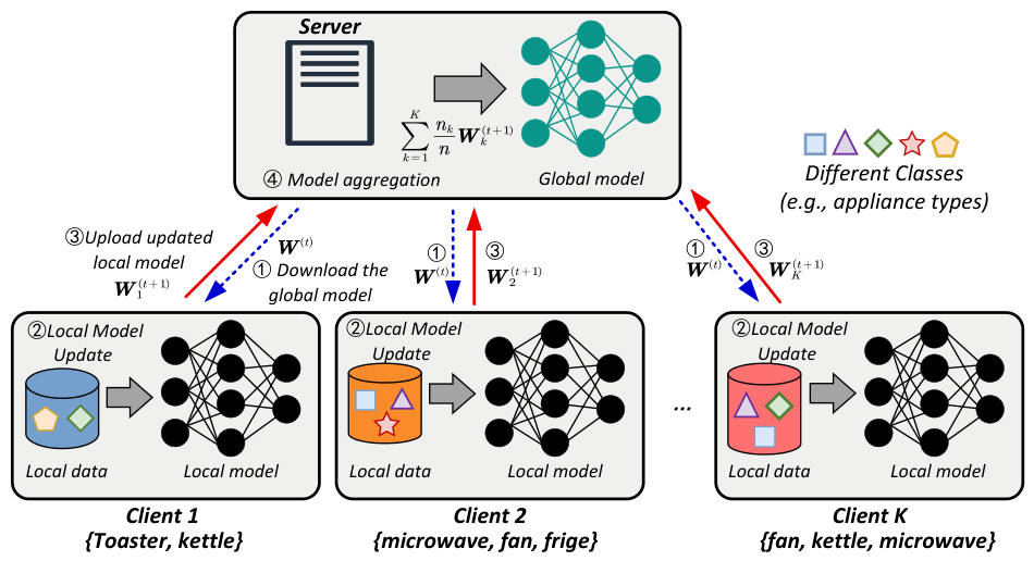
Figure 1 illustrates the typical workflow of an FL process. In the standard FedAvg algorithm, a central server coordinates K clients ${\left\{P_k\right\}}_{k=1}^K$ to collaboratively train a global model. At each communication round t, the server first broadcasts the current global model parameters ${\mathit{W}}^{\left(t\right)}$ to all participating clients. After receiving the global parameters, each client $P_k$ initializes its local model as ${\mathit{W}}_k\leftarrow {\mathit{W}}^{\left(t\right)}$.

Each client $P_k$ then performs local training on its private dataset ${\mathcal{D}}_k={\left\{({\mathbf{x}}_i,y_i)\right\}}_{i=1}^{n_k}$, where ${\mathbf{x}}_i$ denotes the input sample, $y_i$ denotes the corresponding appliance label, and $n_k=\left|{\mathcal{D}}_k\right|$ is the number of local samples. The dataset ${\mathcal{D}}_k$ is assumed to be drawn from the local data distribution ${\mathcal{P}}_k(\mathbf{x},y)$. The local update is carried out over multiple steps of stochastic gradient descent (SGD), typically involving several local epochs. For each step, the model parameters are updated as ${\mathit{W}}_k\leftarrow {\mathit{W}}_k-\eta \nabla {\mathcal{L}}_k\left({\mathit{W}}_k\right)$, where ${\mathit{W}}_k$ denotes the local model parameters of client $P_k$, $\eta$ is the learning rate, $\nabla {\mathcal{L}}_k\left({\mathit{W}}_k\right)$ is the gradient of the local loss with respect to ${\mathit{W}}_k$, and

$${\mathcal{L}}_k\left({\mathit{W}}_k\right)={\displaystyle \frac{1}{n_k}}\sum _{({\mathbf{x}}_i,y_i)\in {\mathcal{D}}_k}\ell (F({\mathbf{x}}_i;{\mathit{W}}_k),y_i).$$

Here, $F({\mathbf{x}}_i;{\mathit{W}}_k)$ denotes the prediction of the local model for input ${\mathbf{x}}_i$, and $\ell (·,·)$ is the task-specific loss function, such as cross-entropy.

After completing local updates, each client uploads its updated parameters ${\mathit{W}}_k$ to the server. The server then aggregates the updates as ${\mathit{W}}^{(t+1)}={\sum }_{k=1}^K{\displaystyle \frac{n_k}{n}}{\mathit{W}}_k$, where $n={\sum }_{k=1}^K{n}_k$ is the total number of training samples. This process is repeated until convergence, with the global objective of minimizing

$$\underset{\mathit{W}}{min}\mathcal{L}\left(\mathit{W}\right)={\displaystyle \sum _{k=1}^K}{\displaystyle \frac{n_k}{n}}{\mathcal{L}}_k\left(\mathit{W}\right).$$

(1)

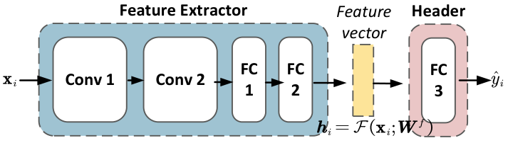
In most FL implementations, the global model $F(\mathbf{x};\mathit{W})$ comprises two components: a feature extractor $\mathcal{F}:{\mathbb{R}}^M\to {\mathbb{R}}^D$ parameterized by ${\mathit{W}}^f$, and a header $\mathcal{H}:{\mathbb{R}}^D\to {\mathbb{R}}^C$ parameterized by ${\mathit{W}}^h$, where $\mathit{W}=\{{\mathit{W}}^f,{\mathit{W}}^h\}$. Here, M, D, and C denote the dimensions of the input space, feature space, and label space, respectively. The model can be expressed as $F(\mathbf{x};\mathit{W})=\mathcal{H}(\mathcal{F}(\mathbf{x};{\mathit{W}}^f);{\mathit{W}}^h)$. We assume that all clients share the same model architecture in this standard HFL setting. Figure 2 illustrates this structure. The terms classifier, header, and head are used interchangeably throughout this paper to denote the same prediction module.

2.2. Problem Statement

In this study, we consider K clients each possessing private electrical measurement datasets. Each client $P_k$ maintains a dataset ${\mathcal{D}}_k={\left\{({\mathbf{x}}_i^k,y_i^k)\right\}}_{i=1}^{n_k}$, where ${\mathbf{x}}_i^k$ represents input features and $y_i^k\in {\mathcal{Y}}_k$ denotes appliance labels. Crucially, label spaces ${\mathcal{Y}}_k$ vary across clients due to differences in available appliances and usage patterns, resulting in ${\mathcal{Y}}_k\ne {\mathcal{Y}}_{k^{\prime }}$ for distinct clients $k\ne k^{\prime }$. For instance, one household might monitor washing machines (WMs), air conditioners (ACs), and televisions, while another tracks only washing machines and laptops, creating label skew. Even for shared appliance types like WMs, usage behaviors often differ substantially, causing feature distribution shifts.

These variations stem from client-specific data distributions $P_k(\mathbf{x},y)$, which introduce two core challenges: feature shift in input space, and heterogeneity in label spaces. This doubly heterogeneous data landscape severely impacts FL. Locally trained models exhibit poor generalization to unseen clients, while centralized approaches compromise data privacy. Classic FL methods like FedAvg further struggle with label space mismatches and distribution discrepancies.

Thus, our objective is to collaboratively train a global model $F(\mathbf{x};\mathit{W})$ without raw data sharing. This model can achieve robust generalization across all clients despite feature distribution shifts and label space heterogeneity, while effectively handling disjoint label sets during inference.

3. Methods

This section describes the overall framework and implementation details of the proposed FedCACP method for addressing the above-mentioned problems.

3.1. Data Acquisition and Preprocessing

For event-based NILM methods, the first step is to detect load switching events, with the aim of disaggregating individual appliances’ voltage and current signals from the aggregated measurements. This paper assumes that, at any given time, only one appliance undergoes a switching event. Such events may either be annotated in the dataset or detected using event detection algorithms that identify significant changes in active power [8,14]. For each detected event, the steady-state voltage and current signals before and after the event are denoted by $(V_{\mathrm{off}},I_{\mathrm{off}})$ and $(V_{\mathrm{on}},I_{\mathrm{on}})$, respectively. The operating voltage and current of the activated appliance are computed as $V_{\mathrm{app}}=V_{\mathrm{on}}$ and $I_{\mathrm{app}}=I_{\mathrm{on}}-I_{\mathrm{off}}$ [8].

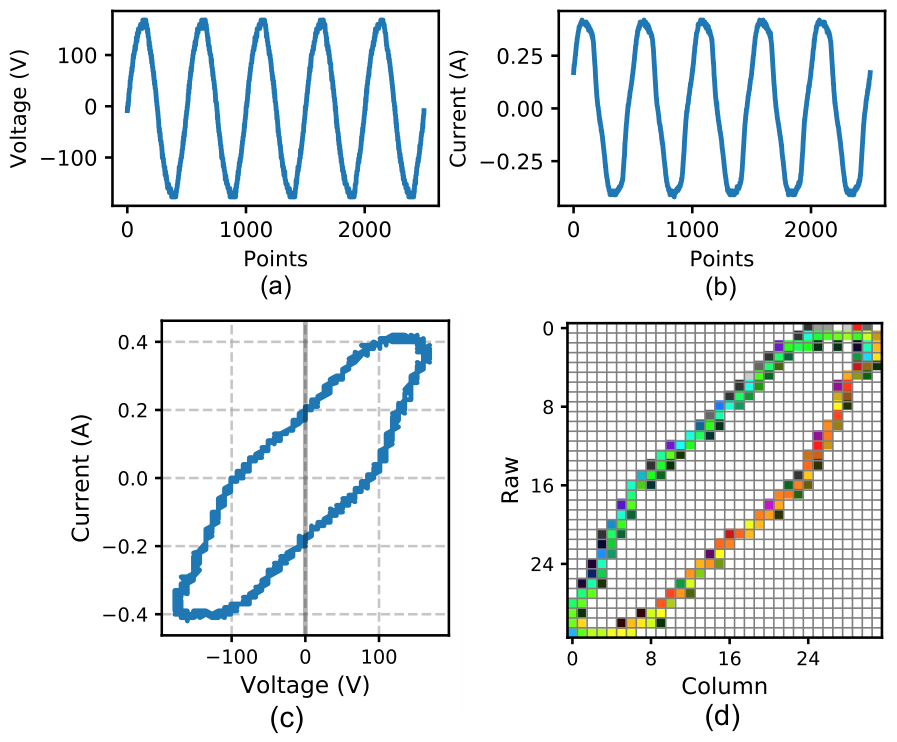
Using $V_{\mathrm{app}}$ and $I_{\mathrm{app}}$, we construct the V-I trajectory of each appliance [10]. The V-I trajectory preserves appliance-specific electrical characteristics, such as phase relationships, nonlinear distortions, and trajectory shapes [13,30]. It is then encoded in the HSV (Hue, saturation, value) color space to produce a compact and discriminative representation [13]. Figure 3 provides an example of this encoding procedure. Figure 3a,b show the voltage and current waveforms of a fan, respectively, while Figure 3c,d illustrate the corresponding V-I trajectory and HSV-encoded trajectory image. Compared with a binary V-I trajectory representation, HSV encoding provides richer information by describing not only the existence of trajectory points but also their spatial distribution and intensity on the V-I plane, which helps preserve discriminative patterns related to appliance operating states.

For each detected event, five steady-state cycles of voltage and current are extracted to construct the V-I trajectory. The voltage and current values are normalized and mapped onto a fixed two-dimensional grid. The accumulated trajectory points are then converted into an HSV image following the encoding procedure in [13]. Therefore, each sample is represented as a three-channel tensor $\mathbf{x}\in {\mathbb{R}}^{3\times 32\times 32}$, where the three channels correspond to hue, saturation, and value, respectively. The resolution of $32\times 32$ follows the setting in [13]. Previous studies [31] have shown that increasing the image resolution beyond this level provides limited improvement while increasing computational cost. Thus, $32\times 32$ is adopted as a trade-off between representation capability and computational efficiency.

To ensure data consistency, all clients within the same dataset use the same event extraction, cycle selection, and HSV V-I trajectory generation procedure. The three datasets are evaluated separately, so samples with different sampling rates are not mixed and no cross-dataset time synchronization is required. Since the public datasets provide complete and labeled event-level voltage/current waveforms, no additional sample removal is performed. An open-source implementation of the HSV-based V-I trajectory generation is available at our GitHub repository (https://github.com/zhz-yan/HSV-VI-NILM; accessed on 20 June 2026).

3.2. Framework Overview

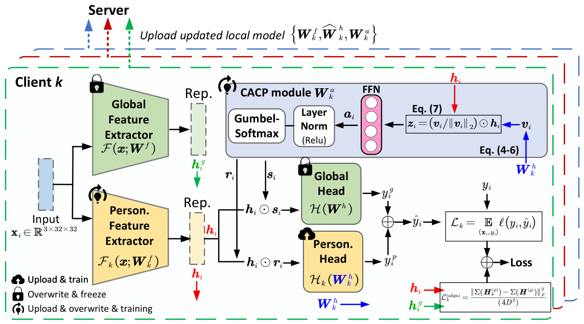
In our framework, each client has a global feature extractor $\mathcal{F}(·)$ and a global head $\mathcal{H}(·)$, parameterized by shared weights ${\mathit{W}}^f$ and ${\mathit{W}}^h$, respectively. In addition, each client maintains a personalized feature extractor ${\mathcal{F}}_k(·)$, a personalized head ${\mathcal{H}}_k(·)$, and a CACP module ${\mathcal{A}}_k(·)$, with parameters ${\mathit{W}}_k^f$, ${\mathit{W}}_k^h$, and ${\mathit{W}}_k^a$, respectively. We assume that all clients share the same network architecture for both global and personalized modules. Figure 4 illustrates the local training process on each client, highlighting the distinction between frozen, trainable, and uploaded components.

At the beginning of communication round t, each client receives the global parameters from the server and initializes its local trainable modules accordingly. Specifically, the adapter parameters are set as ${\mathit{W}}_k^a\leftarrow {\mathit{W}}^{a,\left(t\right)}$, and the personalized feature extractor is initialized as ${\mathit{W}}_k^f\leftarrow {\mathit{W}}^{f,\left(t\right)}$. The global feature extractor $\mathcal{F}(·)$ and the global head $\mathcal{H}(·)$ are kept frozen during local training and serve only as reference modules. Due to distribution shifts, the evolving personalized feature extractor ${\mathcal{F}}_k(·)$ may produce features that are not fully compatible with the frozen global head. Therefore, we align the personalized features with the frozen global features using the CORAL loss [32]. Both the global head $\mathcal{H}(·)$ and the personalized head ${\mathcal{H}}_k(·)$ contribute to the classification loss during training and inference.

Given the local loss ${\mathcal{L}}_k^{\mathrm{total}}\left({\mathit{W}}_k\right)$, the global training objective aggregates local losses weighted by data size:

$$\{{\mathit{W}}_1,\dots ,{\mathit{W}}_K\}=\arg min{\displaystyle \sum _{k=1}^K}{\displaystyle \frac{n_k}{n}}{\mathcal{L}}_k^{\mathrm{total}}\left({\mathit{W}}_k\right),$$

(2)

where minimization occurs over the locally trainable parameters (${\mathit{W}}_k^f$, ${\mathit{W}}_k^h$, ${\mathit{W}}_k^a$) within ${\mathit{W}}_k$.

After local training, each client uploads $\{{\mathit{W}}_k^f,{\widehat{\mathit{W}}}_k^h,{\mathit{W}}_k^a\}$ to the server. Let ${\mathcal{S}}^{\left(t\right)}$ denote the set of clients participating in communication round t, and let $n^{\left(t\right)}={\sum }_{k\in {\mathcal{S}}^{\left(t\right)}}{n}_k^{\left(t\right)}$. The server aggregates these using weighted averaging to update the global parameters for the next round $t+1$:

$$\begin{array}{cc}\hfill & {\mathit{W}}^{f,(t+1)}={\displaystyle \frac{1}{n^{\left(t\right)}}}\sum _{k\in {\mathcal{S}}^{\left(t\right)}}{n}_k^{\left(t\right)}{\mathit{W}}_k^{f,\left(t\right)}\hfill \\ \hfill & {\mathit{W}}^{h,(t+1)}={\displaystyle \frac{1}{n^{\left(t\right)}}}\sum _{k\in {\mathcal{S}}^{\left(t\right)}}{n}_k^{\left(t\right)}{\widehat{\mathit{W}}}_k^{h,\left(t\right)}\hfill \\ \hfill & {\mathit{W}}^{a,(t+1)}={\displaystyle \frac{1}{n^{\left(t\right)}}}\sum _{k\in {\mathcal{S}}^{\left(t\right)}}{n}_k^{\left(t\right)}{\mathit{W}}_k^{a,\left(t\right)}\hfill \end{array}$$

(3)

where ${\widehat{\mathit{W}}}_k^{h,\left(t\right)}=\delta ·{\mathit{W}}_k^{h,\left(t\right)}+(1-\delta )·{\mathit{W}}^{h,\left(t\right)}$ interpolates the locally updated personalized head and the global head distributed by the server at the beginning of communication round t.

In our experiments, all clients participate in each round, i.e., ${\mathcal{S}}^{\left(t\right)}=\{1,\dots ,K\}$, and the client ratio is 1.0. Therefore, $n_k^{\left(t\right)}$ is equal to the number of local training samples of client k in round t. If client dropout or offline clients are considered, the same aggregation rule can be applied only over the participating client set ${\mathcal{S}}^{\left(t\right)}$, and $n^{\left(t\right)}$ is recomputed accordingly.

3.3. Model Components

3.3.1. Feature Extractor

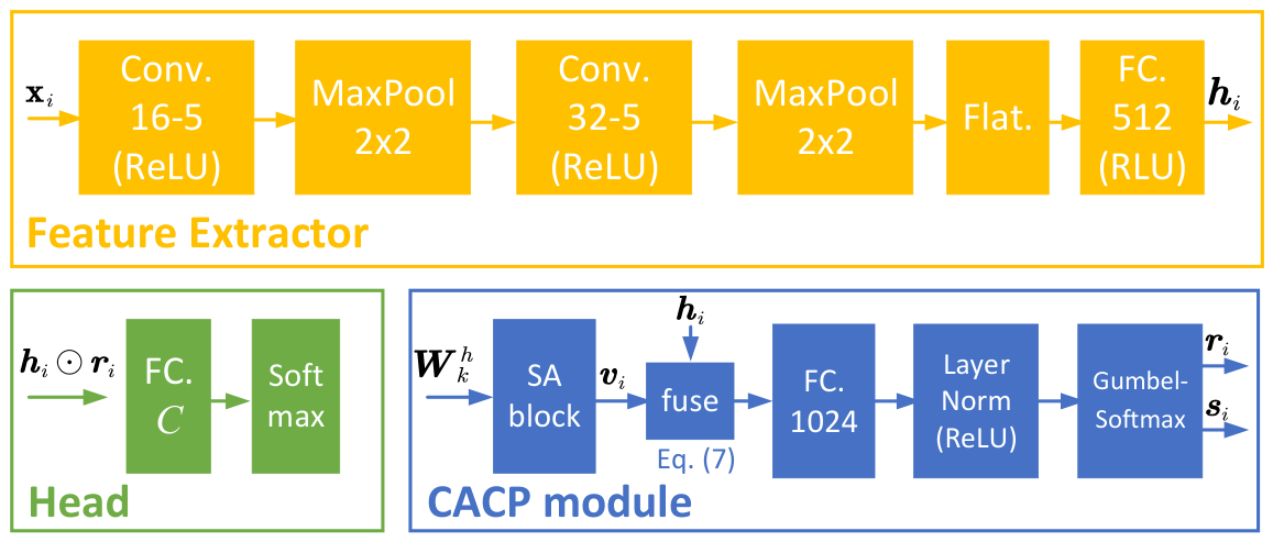
We now present the detailed design of each module. As shown in Figure 4, let ${\mathit{h}}_i={\mathcal{F}}_k\left({\mathbf{x}}_i\right)$ denote the feature vector (representations, rep.) extracted by the personalized feature extractor for each sample $({\mathbf{x}}_i,y_i)\in D_k$. Due to statistical heterogeneity, the representation ${\mathit{h}}_i\in {\mathbb{R}}^D$ extracted by ${\mathcal{F}}_k(·)$ contains a mixture of global and client-specific information. To disentangle these components, we introduce the CACP module, which generates sample-specific separation policies in a fully data-driven manner. By leveraging the outputs from both the frozen global head $\mathcal{H}(·)$ and the adaptive personalized head ${\mathcal{H}}_k(·)$, the CACP module identifies which features should contribute to global learning and which should remain local. Figure 5 illustrates the proposed neural network architecture. In the figure, Conv.16-5 denotes a two-dimensional convolutional layer with 16 filters and a $5\times 5$ kernel. FC, ReLU, and SA denote the fully connected layer, rectified linear unit, and self-attention, respectively.

3.3.2. Context-Aware Conditional Policy (CACP) Module

Conditional computation refers to the technique of activating only a subset of units in a network based on input-dependent conditions [33]. Inspired by [34,35,36], we introduce a CACP module as an auxiliary policy network that dynamically generates sample-specific gating vectors to route feature components to global or personalized heads.

To capture the client-specific context needed to guide the separation of global and personalized features within ${\mathit{h}}_i$, we utilize the weight matrix from personalized head ${\mathit{W}}_k^h\in {\mathbb{R}}^{C\times D}$. The CACP module ${\mathcal{A}}_k(·)$ (parameterized by ${\mathit{W}}_k^a$) processes this information through self-attention (SA), followed by a feedforward network. We interpret ${\mathit{W}}_k^h$ as C token embeddings (each $\in {\mathbb{R}}^D$) and apply scaled dot-product self-attention:

$$\mathit{Q}={\mathit{W}}_k^h{\mathit{W}}^Q,\mathit{K}={\mathit{W}}_k^h{\mathit{W}}^K,\mathit{V}={\mathit{W}}_k^h{\mathit{W}}^V$$

(4)

where ${\mathit{W}}^Q,{\mathit{W}}^K,{\mathit{W}}^V\in {\mathbb{R}}^{D\times D}$ are client-specific trainable matrices.

The attention output is computed as follows:

$$\mathrm{AttnOut}(\mathit{Q},\mathit{K},\mathit{V})=\mathrm{Softmax}\left({\displaystyle \frac{\mathit{Q}{\mathit{K}}^{\top }}{\sqrt{D}}}\right)\mathit{V}$$

(5)

We compute a client-context vector ${\mathit{v}}_k$ by averaging the attention output vectors across the C class tokens:

$${\mathit{v}}_k={\displaystyle \frac{1}{C}}{\displaystyle \sum _{c=1}^C}{\mathrm{AttnOut}}_c\in {\mathbb{R}}^D.$$

(6)

This vector encapsulates client-specific information from ${\mathit{W}}_k^h$. We compute ${\mathit{v}}_k$ once at the start of each local training epoch and keep it fixed during subsequent local updates. During inference, we use the latest ${\mathit{v}}_k$.

For each sample ${\mathbf{x}}_i$, we form a fused representation combining the client context and its feature vector:

$${\mathit{z}}_i=\left({\displaystyle \frac{{\mathit{v}}_k}{{∥{\mathit{v}}_k∥}_2}}\right)\odot {\mathit{h}}_i,$$

(7)

where ⊙ denotes the Hadamard (element-wise) product and ${∥·∥}_2$ is the ${\ell }_2$-norm.

To disentangle the global and personalized components within ${\mathit{h}}_i$, we generate gating logits using a client-specific feedforward network (FFN) applied to ${\mathit{z}}_i$:

$${\mathit{a}}_i=\mathrm{FFN}\left({\mathit{z}}_i\right)\in {\mathbb{R}}^{D\times 2}.$$

(8)

Let ${\mathit{a}}_i^{\left(d\right)}=[a_{i,d}^{\left(1\right)},a_{i,d}^{\left(2\right)}]$ denote the logits for feature dimension $d=1,\dots ,D$. Using Gumbel-Softmax for differentiable sampling [37], the gating values are

$$r_i^{\left(d\right)}={\displaystyle \frac{exp((a_{i,d}^{\left(1\right)}+g_{i,d}^{\left(1\right)})/\tau )}{{\sum }_{j=1}^{2}exp((a_{i,d}^{\left(j\right)}+g_{i,d}^{\left(j\right)})/\tau )}},s_i^{\left(d\right)}={\displaystyle \frac{exp((a_{i,d}^{\left(2\right)}+g_{i,d}^{\left(2\right)})/\tau )}{{\sum }_{j=1}^{2}exp((a_{i,d}^{\left(j\right)}+g_{i,d}^{\left(j\right)})/\tau )}}$$

(9)

where $g_{i,d}^{\left(j\right)}$ denotes the Gumbel noise and $\tau$ is the temperature parameter. The gates satisfy $r_i^{\left(d\right)}+s_i^{\left(d\right)}=1$, and the corresponding gating vectors are ${\mathit{r}}_i={[r_i^{\left(1\right)},\dots ,r_i^{\left(D\right)}]}^{\top }$ and ${\mathit{s}}_i={[s_i^{\left(1\right)},\dots ,s_i^{\left(D\right)}]}^{\top }$.

In this work, the temperature parameter is set to $\tau =1.0$ with soft sampling. This setting follows the standard Gumbel-Softmax configuration [34] and provides a moderate temperature that balances differentiable optimization and effective feature routing. The CACP module aims to learn soft feature-wise gating weights rather than hard discrete routing decisions; therefore, $\tau =1.0$ helps maintain stable gradient-based optimization while still allowing the model to distinguish between global and personalized feature components. A smaller $\tau$ would generate sharper and more discrete gates, which may introduce unstable local updates, whereas a larger $\tau$ would produce overly smooth gates and weaken the separation between global and personalized representations.

3.3.3. Header

Finally, we decompose the original feature vector ${\mathit{h}}_i$ into global and personalized components using the following gating vectors:

$${\mathit{z}}_i^{\left(g\right)}={\mathit{r}}_i\odot {\mathit{h}}_i,{\mathit{z}}_i^{\left(p\right)}={\mathit{s}}_i\odot {\mathit{h}}_i.$$

(10)

These components are fed into the global head $\mathcal{H}(·)$ and the personalized head ${\mathcal{H}}_k(·)$, respectively:

$$y_i^g=\mathcal{H}({\mathit{z}}_i^{\left(g\right)};{\mathit{W}}^h),y_i^p={\mathcal{H}}_k({\mathit{z}}_i^{\left(p\right)};{\mathit{W}}_k^h).$$

(11)

The final prediction for sample ${\mathbf{x}}_i$ is the sum of these outputs:

$${\widehat{y}}_i:=y_i^g+y_i^p.$$

(12)

The local loss function for client k is the average cross-entropy loss over its local dataset $D_k$:

$${\mathcal{L}}_k={\displaystyle \frac{1}{|D_k|}}\sum _{({\mathbf{x}}_i,y_i)\in D_k}\ell (y_i,{\widehat{y}}_i)$$

(13)

where $\ell (·,·)$ is the cross-entropy loss. It is worth noting that the output dimension of both heads is defined over the global label space $\mathcal{Y}={\cup }_{k=1}^K{\mathcal{Y}}_k$. During local training, logits corresponding to locally missing classes are not masked. Instead, the standard softmax cross-entropy is computed over the full global label space. For a local sample, only its ground-truth class contributes as the positive target, while the logits of locally absent classes participate in the softmax normalization and receive gradients indirectly.

After local training in round t, client k prepares the head parameters for uploading by interpolating the locally updated personalized head and the global head received at the beginning of the same communication round:

$${\widehat{\mathit{W}}}_k^{h,\left(t\right)}=\delta ·{\mathit{W}}_k^{h,\left(t\right)}+(1-\delta )·{\mathit{W}}^{h,\left(t\right)},$$

(14)

where ${\mathit{W}}^{h,\left(t\right)}$ denotes the global head distributed by the server at the beginning of communication round t, and ${\mathit{W}}_k^{h,\left(t\right)}$ denotes the locally updated personalized head after local training in round t. The parameter $\delta \in [0,1]$ controls the contribution of the personalized head to the uploaded head. Client k uploads the set $\left\{{\mathit{W}}_k^{f,\left(t\right)},{\widehat{\mathit{W}}}_k^{h,\left(t\right)},{\mathit{W}}_k^{a,\left(t\right)}\right\}$ to the server.

3.4. Feature Alignment Strategy

During local training, the evolving personalized feature extractor ${\mathcal{F}}_k(·)$ may produce representations that are misaligned with the frozen global head. To maintain compatibility and enhance cross-client generalization, we align the output features of the personalized extractor with those of the frozen global extractor using the Correlation Alignment (CORAL) loss. Specifically, for a local mini-batch or local dataset, we define ${\mathit{H}}_k^{\left(p\right)}={\left\{{\mathcal{F}}_k({\mathbf{x}}_i;{\mathit{W}}_k^f)\right\}}_{i=1}^{n_k}$ as the personalized feature set, and ${\mathit{H}}^{\left(g\right)}={\left\{\mathcal{F}({\mathbf{x}}_i;{\mathit{W}}^{f,\left(t\right)})\right\}}_{i=1}^{n_k}$ as the feature set generated by the frozen global feature extractor received at the beginning of communication round t. The CORAL loss is then computed as

$${\mathcal{L}}_k^{\mathrm{align}}={\displaystyle \frac{1}{4D^2}}{∥\Sigma \left({\mathit{H}}_k^{\left(p\right)}\right)-\Sigma \left({\mathit{H}}^{\left(g\right)}\right)∥}_F^2,$$

(15)

where $\Sigma (·)$ computes the empirical covariance matrix, D is the feature dimension, and ${\parallel ·\parallel }_F$ denotes the Frobenius norm. The factor $4D^2$ follows the standard Deep CORAL formulation and normalizes the covariance discrepancy with respect to the feature dimension. Since the Frobenius norm sums over $D^2$ covariance entries, this normalization prevents the alignment loss from scaling with D.

The complete local training objective combines the classification loss and the alignment term:

$${\mathcal{L}}_k^{\mathrm{total}}={\displaystyle \frac{1}{|D_k|}}\sum _{({\mathbf{x}}_i,y_i)\in D_k}\ell (y_i,{\widehat{y}}_i)+\lambda ·{\mathcal{L}}_k^{\mathrm{align}}$$

(16)

where ${\widehat{y}}_i$ is the fused prediction defined in Equation (12).

The complete training procedure of FedCACP is summarized in Algorithm 1, including server-side broadcasting, client-side local training, head interpolation, and server-side aggregation.

Algorithm 1: FedCACP

4. Experimental Setup

This section presents the setup used to evaluate the proposed method, including the datasets, performance indicators, comparison methods, and case settings.

4.1. Dataset Description

We evaluated the proposed method on three public NILM datasets: PLAID [38], WHITED [39], and COOLL [40]. All of these datasets provide high-frequency voltage and current measurements from a variety of appliance types.

• PLAID: Contains 1793 voltage and current waveforms sampled at 30 kHz, covering 11 appliance types collected from over 50 U.S. households.
• WHITED: Provides 1100 sub-metered measurements sampled at 44 kHz, covering 46 appliance types. Each type includes 1 to 9 brands, and each brand has 10 recorded start-up events.
• COOLL: Contains 42 appliance instances spanning 12 appliance types. Each appliance instance has 20 turn-on transient signals recorded with varied delays relative to the mains voltage zero-crossing. All signals are sampled at 100 kHz.

4.2. Performance Indicators

To evaluate classification performance, we adopt standard metrics: accuracy, precision, recall, and F1-score. Accuracy is defined as

$$\mathrm{Accuracy}={\displaystyle \frac{TP+TN}{TP+TN+FN+FP}}$$

(17)

where $TP$, $TN$, $FP$, and $FN$ are true positives, true negatives, false positives, and false negatives, respectively.

For multiclass evaluation, we compute the F1-score per class and report the macro-average. For class i, the F1-score is given by

$$F{1}_i={\displaystyle \frac{2·Pr{e}_i·Re{c}_i}{Pr{e}_i+Re{c}_i}},$$

(18)

with precision $Pr{e}_i={\displaystyle \frac{T{P}_i}{T{P}_i+F{P}_i}}$ and recall $Re{c}_i={\displaystyle \frac{T{P}_i}{T{P}_i+F{N}_i}}$. The macro F1-score is then $F_{\mathrm{macro}}={\displaystyle \frac{1}{C}}{\sum }_{i=1}^{C}F{1}_i$.

Since each experiment was repeated 10 times unless otherwise specified, we further conducted statistical significance testing to assess whether the improvements of FedCACP over the strongest baselines were due to random variation. For each dataset and experimental setting, FedCACP was compared with the baseline methods using Welch’s one-sided t-test, where the alternative hypothesis was that FedCACP achieves better performance than the baseline. Welch’s test was adopted because different methods may have unequal variances across repeated runs. Bonferroni correction was applied within each group of baseline comparisons, and a corrected p-value smaller than 0.05 was considered statistically significant. In addition, 95% confidence intervals were computed as

$${\mathrm{CI}}_{95\%}=\overline{x}\pm t_{0.975,n-1}{\displaystyle \frac{s}{\sqrt{n}}},$$

(19)

where $\overline{x}$, s, and n denote the mean, standard deviation, and number of independent runs, respectively.

4.3. Comparison Methods

To verify the effectiveness of the proposed approach, we evaluated the following groups of methods:

1.

Centralized Baselines: For the centralized setting, we selected four state-of-the-art load identification methods that have demonstrated strong performance in prior evaluations. These included Random Forest (RF) [9,14] (https://github.com/jingkungao/PLAID; accessed on 20 June 2026), HSV V-I Trajectory (V-I) [10,13] (https://github.com/zhz-yan/HSV-VI-NILM; accessed on 20 June 2026), Adaptive Weighted Recurrence Graphs (AWRG) [31] (https://github.com/sambaiga/AWRGNILM; accessed on 20 June 2026), and Learnable Image-Based Load Signature (LILS) [41] (https://github.com/Deep-fishing/ALILS; accessed on 20 June 2026). In both Case 1 and Case 3, all models were implemented following the original papers, with experimental setups aligned with the papers’ descriptions and available code.

2.

Federated Baselines: We adopted FedAvg [21] (https://github.com/alexbie98/fedavg; accessed on 20 June 2026) and FedProx [42] as the federated learning strategies to evaluate the performance of existing methods in distributed settings. FedAvg has been widely used in prior federated NILM studies as a standard aggregation strategy [16,18,20,22,26,27], while FedProx is designed to address data heterogeneity in non-IID federated scenarios [23]. For evaluation, each centralized baseline was integrated with both FedAvg and FedProx to form its federated counterpart. For example, FedAvg (AWRG) denotes the AWRG model trained using the FedAvg strategy. All federated models were trained under the same communication rounds and local update settings to ensure fair comparison.

Implementation Details: The input was an HSV-encoded V-I trajectory image of size $(3,32,32)$, selected to balance representation capability and model complexity [13,43]. As shown in Figure 5, the feature extractor contained two 2-D convolutional layers with 16 and 32 filters, both using a $5\times 5$ kernel, stride 1, and no padding, each followed by $2\times 2$ max pooling. The flattened feature map was passed to a 512-unit fully connected layer, giving a feature dimension of $D=512$. The head was a fully connected layer of size C followed by softmax. The CACP module consisted of a 2-head self-attention block, the fusion operation in Equation (7), a 1024-unit FC layer with layer normalization and ReLU, and a Gumbel-Softmax layer with $\tau =1.0$ to generate ${\mathit{r}}_i$ and ${\mathit{s}}_i$. Models were trained using SGD with batch size 32 and learning rate 0.001. We used $K=5$ clients, full client participation, 150 communication rounds, and 10 local epochs per round. Thus, the reported results correspond to the full-participation setting, while client dropout or offline participation is left for future work. All experiments were conducted on an NVIDIA GeForce RTX 4060 GPU, repeated 10 times, and reported as the mean ± standard deviation.

4.4. Case Settings

We evaluated our approach under four scenarios:

1.

Case 1: All clients share IID data, with local datasets independently sampled from the same global distribution. This configuration simulates an ideal centralized scenario where data heterogeneity is absent, serving as a performance baseline.

2.

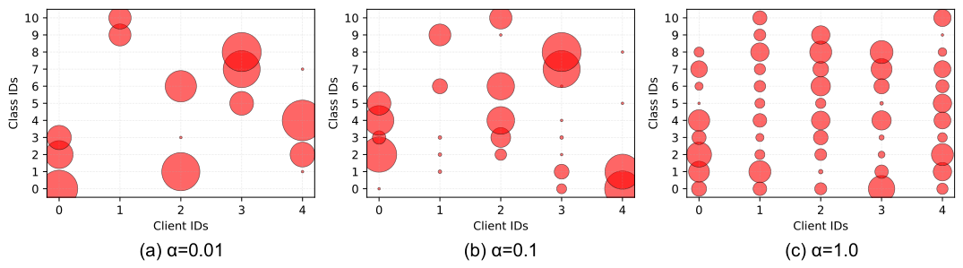
Case 2: We simulate non-IID settings using Dirichlet sampling with parameter $\alpha \in \{0.01,0.1,1.0\}$ to control non-IID intensity. For each client k, a class distribution vector $p_k^{\left(c\right)}\sim \mathrm{Dir}\left(\alpha \right)$ is sampled, with smaller $\alpha$ values producing stronger per-client class imbalance. An illustration of non-IID client data distributions on the PLAID dataset with varying Dirichlet parameter $\alpha$ is provided in Figure 6.

3.

Case 3: House-Partitioned Clients: Each client is associated with a unique residential house, and all appliances from that house are exclusively assigned to the same client. Within each house, an 80/20 train–test split is applied locally to preserve data locality and enable personalized evaluation. For PLAID, the house-partitioned setting is constructed directly using the original household metadata. However, WHITED and COOLL do not provide household identifiers. Therefore, following the protocol used in previous studies [10], we generate virtual houses by randomly assigning appliance instances of each appliance type to different houses. All measurements from the same appliance instance are kept in the same virtual house to avoid event-level leakage. The number of virtual houses is set to 9 for WHITED and 8 for COOLL, corresponding to the maximum number of appliance instances among all appliance types in each dataset. Appliance types with only one appliance instance are excluded because they cannot support house-level partitioning. Thus, the results on WHITED and COOLL should be interpreted as evaluations under simulated client-level heterogeneity rather than real household-level splits.

4.

Case 4: Leave-One-House-Out Cross-Validation (LoHoCV) Generalization: For each target house $h\in \{1,\dots ,H\}$, the remaining $H-1$ houses are assigned to $K=H-1$ clients for federated training. The model is then evaluated exclusively on house h. This process is repeated for all H houses, and the final performance is averaged over all folds. This evaluation is conducted solely on the PLAID dataset due to its house-level metadata.

5. Results and Discussion

5.1. Parameter Studies

We conducted ablation and hyperparameter studies to evaluate the impact of key components in our method. Unless otherwise specified, all experiments in this subsection were performed under a non-IID setting using Dirichlet sampling with $\alpha =0.1$ for consistent comparison.

5.1.1. Ablation Study

We evaluated the contribution of each module through an ablation study on the PLAID dataset, as shown in

Table 1. Ablation study results on the PLAID dataset.

Method	F1-Macro	Precision	Recall
Proposed	93.8 ± 0.8	94.3 ± 0.8	93.9 ± 0.8
w/o CACP	89.5 ± 3.1	90.4 ± 2.9	89.9 ± 3.1
w/o CACP & CL	85.2 ± 1.8	86.7 ± 1.7	86.8 ± 1.5
w/o CACP & CL & GH	88.9 ± 1.5	90.1 ± 1.4	89.7 ± 1.6
w/o CACP & GH	87.3 ± 2.9	88.3 ± 2.5	88.4 ± 2.8
w/o CL	88.1 ± 2.3	89.2 ± 2.2	88.7 ± 2.3

Note: CACP: Context-Aware Conditional Policy; CL: CORAL-based feature alignment loss; GH: global head; F1-macro: Macro-averaged F1-score.

. Removing the CACP module (w/o CACP) led to a clear performance drop, with F1-macro decreasing from 93.8% to 89.5%. Further removing the CORAL loss (w/o CACP & CL) reduced the performance to 85.2%, confirming the importance of feature alignment.

Further removing the global head (w/o CACP & CL & GH) slightly improved performance compared to removing only CACP and CORAL loss, with F1-macro increasing from 85.2% to 88.9%. This indicates that the global head may introduce interference when the alignment mechanism is absent. In contrast, removing only the CORAL loss (w/o CL) had a smaller effect, suggesting that the CACP module is the primary contributor to the observed performance gain.

5.1.2. Effect of $\delta$

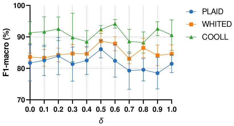
We evaluated the effect of the interpolation coefficient $\delta$, which controls the balance between the global and personalized heads. As illustrated in Figure 7, both extremes—using only the global head ($\delta =0$) or only the personalized head ($\delta =1$)—led to suboptimal performance across all datasets. Intermediate values of $\delta$ consistently yielded better results. For PLAID and WHITED, the highest F1-macro was observed around $\delta =0.6$, while COOLL achieved robust performance across a broader range of $\delta \in [0.4, 0.8]$, with relatively low variance. These findings suggest that a moderate blend of global and personalized representations is beneficial.

Although the best value of $\delta$ varied slightly across datasets, the performance remained relatively stable within the middle range. For example, PLAID and WHITED achieved the best F1-macro around $\delta =0.6$, while COOLL maintained robust performance over a wider interval. To avoid dataset-specific tuning and ensure a unified experimental setting, we set $\delta =0.5$ for all subsequent experiments as a balanced choice between global aggregation and local personalization. An adaptive strategy for selecting $\delta$ according to client heterogeneity is a promising direction for future work.

5.1.3. Effect of the Alignment Loss Weight $\lambda$

Table 2. Sensitivity analysis of the alignment loss weight $\lambda$ under Case 2 with $\alpha =0.1$. The reported values are F1-macro (%).

Dataset	$\mathit{\lambda }=0$	$\mathit{\lambda }=0.001$	$\mathit{\lambda }=0.01$	$\mathit{\lambda }=0.1$	$\mathit{\lambda }=1$
PLAID	$92.20\pm 1.57$	$92.16\pm 1.35$	$92.34\pm 1.19$	$92.46\pm 1.14$	$91.94\pm 1.07$
WHITED	$94.26\pm 1.85$	$94.45\pm 1.62$	$94.28\pm 1.53$	$94.06\pm 2.00$	$94.54\pm 1.61$
COOLL	$98.12\pm 1.36$	$98.18\pm 1.38$	$97.98\pm 1.32$	$98.09\pm 1.41$	$98.12\pm 1.49$

reports the sensitivity analysis of the alignment loss weight $\lambda$. FedCACP shows stable F1-macro across different $\lambda$ values on all three datasets, with variations generally within the standard deviations. This indicates that FedCACP is not highly sensitive to $\lambda$, and that the CORAL-based alignment term mainly serves as a regularizer for improving feature compatibility.

Although different datasets show slightly different optimal values, all tested $\lambda$ values led to comparable performance. In particular, the default setting $\lambda =1$ used in the main experiments achieved competitive results on all three datasets, with F1-macro scores of 91.94%, 94.54%, and 98.12% on PLAID, WHITED, and COOLL, respectively. Therefore, we kept $\lambda =1$ in the main experiments for consistency.

5.2. Results in Case 1 (IID)

Table 3. Experimental results in Case 1.

Method	PLAID		WHITED		COOLL
	Accuracy	F1-Macro	Accuracy	F1-Macro	Accuracy	F1-Macro
Central (RF)	97.5 ± 0.3	96.8 ± 0.3	99.3 ± 0.3	99.2 ± 0.3	96.4 ± 0.5	96.5 ± 0.7
Central (LILS)	94.0 ± 0.9	92.9 ± 1.1	92.3 ± 0.7	91.7 ± 1.1	84.1 ± 2.0	83.5 ± 2.3
Central (V-I)	93.9 ± 0.4	92.4 ± 0.6	95.7 ± 0.5	95.4 ± 0.7	97.7 ± 0.6	97.9 ± 0.5
Central (AWRG)	95.4 ± 0.8	94.2 ± 0.8	91.7 ± 0.5	88.8 ± 0.7	91.9 ± 0.8	94.1 ± 0.6
FedAvg (LILS)	93.1 ± 3.0	92.2 ± 3.0	93.1 ± 2.9	92.3 ± 2.9	88.7 ± 5.0	88.3 ± 6.6
FedAvg (V-I)	95.3 ± 0.8	93.9 ± 1.1	96.3 ± 0.9	96.3 ± 1.2	99.1 ± 0.9	99.2 ± 0.8
FedAvg (AWRG)	88.7 ± 2.5	86.5 ± 3.1	82.1 ± 2.7	79.9 ± 3.5	87.3 ± 2.8	90.1 ± 2.5
FedProx (LILS)	88.8 ± 1.3	86.5 ± 1.9	91.6 ± 1.7	91.3 ± 2.3	89.1 ± 2.5	90.5 ± 2.9
FedProx (V-I)	90.6 ± 1.1	88.7 ± 1.4	93.3 ± 1.0	92.6 ± 0.9	96.5 ± 1.5	96.7 ± 1.5
FedProx (AWRG)	93.4 ± 1.3	91.7 ± 1.3	90.0 ± 2.1	88.8 ± 2.9	93.2 ± 2.2	94.6 ± 1.6
FedCACP	95.7 ± 1.0	94.5 ± 1.3	96.3 ± 1.1	95.3 ± 1.7	99.5 ± 0.4	99.4 ± 0.4

Note: Accuracy denotes accuracy. RF: Random Forest; V-I: voltage–current trajectory; AWRG: Adaptive Weighted Recurrence Graphs; LILS: Learnable Image-Based Load Signature. FedAvg: Federated Averaging; FedProx: Federated Proximal; FedCACP: Federated Context-Aware Conditional Policy. The notations “FedAvg (X)” and “FedProx (X)” denote the X-based appliance recognition models trained using FedAvg and FedProx, respectively.

reports the results under Case 1. As expected, centralized methods performed strongly in this homogeneous setting. On PLAID, central (RF) achieved the best performance, with $97.5 \pm 0.3\%$ accuracy and $96.8 \pm 0.3\%$ F1-macro. Among image-based representations, central (AWRG), central (LILS), and central (V-I) achieved F1-macro scores of $94.2\pm 0.8\%$, $92.9\pm 1.1\%$, and $92.4\pm 0.6\%$, respectively. These results confirm the advantage of direct data sharing when distributional shifts are absent.

Federated baselines generally performed worse, especially under FedAvg. For example, FedAvg (AWRG) achieved only $86.5\pm 3.1\%$ F1-macro on PLAID, revealing performance degradation even in IID conditions. This suggests that local inconsistency and limited personalization hinder learning despite aligned distributions. FedProx improves some variants, but its performance still depends strongly on the input representation. For example, on COOLL, FedProx (V-I) reached $96.7\pm 1.5\%$ F1-macro, whereas FedProx (LILS) achieved $90.5\pm 2.9\%$.

The proposed FedCACP method consistently achieved strong performance across datasets, with F1-macro scores of $94.5\pm 1.3\%$, $95.3\pm 1.7\%$, and $99.4\pm 0.4\%$ on PLAID, WHITED, and COOLL, respectively. Notably, it maintained low variance, demonstrating its effectiveness in learning robust representations even under ideal conditions.

5.3. Results in Case 2 (Non-IID Data)

Table 4. Comparison of average test accuracy (%) under Dirichlet distribution in the FL setting with different $\alpha$.

Method	PLAID			WHITED			COOLL
	$\mathit{\alpha }=\mathbf{0.01}$	$\mathit{\alpha }=\mathbf{0.1}$	$\mathit{\alpha }=\mathbf{1.0}$	$\mathit{\alpha }=\mathbf{0.01}$	$\mathit{\alpha }=\mathbf{0.1}$	$\mathit{\alpha }=\mathbf{1.0}$	$\mathit{\alpha }=\mathbf{0.01}$	$\mathit{\alpha }=\mathbf{0.1}$	$\mathit{\alpha }=\mathbf{1.0}$
FedAvg (LILS)	63.5 ± 2.1	64.6 ± 1.8	87.6 ± 1.6	47.1 ± 3.2	54.4 ± 3.7	84.6 ± 3.7	55.1 ± 1.9	63.5 ± 2.9	89.1 ± 3.4
FedAvg (V-I)	89.0 ± 2.2	87.4 ± 1.4	92.8 ± 0.9	89.7 ± 1.5	89.9 ± 1.3	95.3 ± 0.6	83.9 ± 1.0	89.5 ± 1.4	97.6 ± 0.8
FedAvg (AWRG)	67.2 ± 1.2	65.9 ± 2.8	87.9 ± 0.9	47.4 ± 2.2	48.3 ± 3.2	77.4 ± 5.0	45.9 ± 1.3	52.7 ± 3.9	68.6 ± 2.7
FedProx (LILS)	64.0 ± 7.4	70.3 ± 7.2	94.4 ± 0.9	48.9 ± 4.6	49.9 ± 5.8	91.2 ± 2.5	37.4 ± 8.9	36.9 ± 4.5	78.9 ± 5.9
FedProx (V-I)	71.0 ± 8.4	82.1 ± 4.0	92.3 ± 1.8	81.9 ± 5.0	87.1 ± 2.0	94.9 ± 0.8	58.9 ± 8.3	75.6 ± 7.0	96.0 ± 2.2
FedProx (AWRG)	52.7 ± 9.9	60.4 ± 8.9	91.2 ± 1.2	40.4 ± 6.7	46.8 ± 2.9	88.5 ± 1.6	35.2 ± 5.6	46.4 ± 7.4	83.2 ± 4.4
FedCACP	93.8 ± 1.1	93.8 ± 0.9	93.6 ± 1.8	94.3 ± 1.3	92.3 ± 1.4	95.9 ± 1.2	93.8 ± 0.7	96.6 ± 1.5	99.1 ± 0.8

reports the Case 2 results under Dirichlet non-IID settings. Severe heterogeneity substantially degrades standard FL methods, especially when $\alpha =0.01$. For example, on PLAID, FedAvg (LILS) and FedProx (LILS) achieved only 63.5% and 64.0% accuracy, respectively, while FedProx (V-I) performed better, with 71.0%. As $\alpha$ increases, the data distribution becomes more balanced and most methods improve. However, FedProx does not consistently outperform FedAvg under strong skew, indicating that proximal regularization alone is insufficient for this setting. The Dirichlet setting partially reflects long-tailed appliance usage, where smaller $\alpha$ values produce stronger within-client and across-client class imbalance. FedCACP does not explicitly suppress minority classes because all classes remain in the global output space and the CACP module uses sample-wise, rather than class-frequency-based, gating. Nevertheless, extremely rare classes may still have unstable representations, motivating future work on focal loss or minority-aware aggregation.

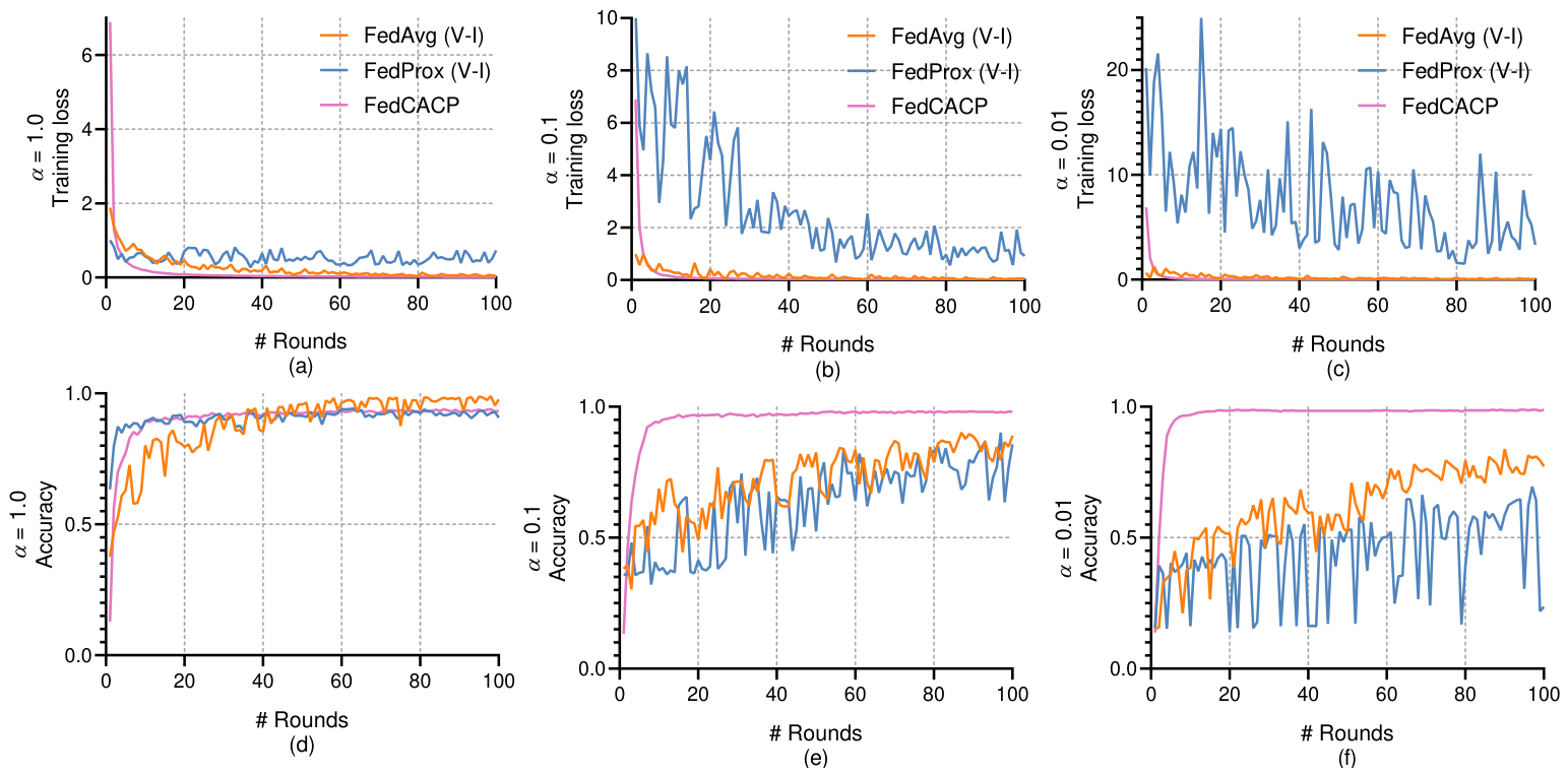
Figure 8 compares the training dynamics of FedAvg, FedProx, and FedCACP under Dirichlet-based non-IID data partitions. The left column shows the training loss, while the right column shows the test accuracy. Subfigures (a,b), (c,d), and (e,f) correspond to $\alpha =1.0$, $\alpha =0.1$, and $\alpha =0.01$, respectively. When $\alpha =1.0$ (i.e., the data distribution is nearly IID), baseline methods such as FedAvg and FedProx achieve competitive performance. However, as the non-IID level increases (smaller $\alpha$), their training becomes unstable and ineffective, as evidenced by the rising loss and degraded accuracy curves. Most notably, FedCACP consistently surpassed all baselines under the most challenging condition $\alpha =0.01$, achieving 93.8%, 94.3%, and 93.8% accuracy on PLAID, WHITED, and COOLL, respectively. These results highlight the effectiveness of our context-aware conditional policy and alignment regularization in addressing client drift and maintaining generalization under severe non-IID conditions.

The statistical tests further confirm the robustness of FedCACP under highly non-IID settings. For the representative case highlighted by the reviewer—namely, PLAID with $\alpha =0.01$—FedCACP achieved $93.8\pm 1.1\%$ accuracy, corresponding to a 95% confidence interval of $[93.01, 94.59]\%$, while the strongest baseline, FedAvg (V-I), achieved $89.0 \pm 2.2\%$, corresponding to a 95% confidence interval of $[87.43, 90.57]\%$. These two confidence intervals do not overlap, indicating that the observed gain is unlikely to be caused by random variation.

5.4. Results in Case 3

Table 5. Experimental results in Case 3.

Method	PLAID		WHITED		COOLL
	Accuracy	F1-Macro	Accuracy	F1-Macro	Accuracy	F1-Macro
FedAvg (LILS)	90.1 ± 2.9	88.9 ± 3.4	51.6 ± 7.8	22.1 ± 5.4	69.2 ± 6.9	46.7 ± 9.6
FedAvg (V-I)	87.4 ± 5.3	85.3 ± 4.7	94.9 ± 1.3	93.3 ± 2.9	96.0 ± 3.0	94.9 ± 4.9
FedAvg (AWRG)	84.5 ± 2.1	82.0 ± 3.2	62.1 ± 9.8	55.2 ± 15.3	33.4 ± 5.5	14.2 ± 4.8
FedProx (LILS)	22.5 ± 7.8	15.7 ± 8.9	12.9 ± 5.1	5.4 ± 3.2	16.9 ± 4.9	4.7 ± 3.1
FedProx (V-I)	92.4 ± 1.6	91.0 ± 1.7	93.2 ± 5.2	90.8 ± 7.8	93.5 ± 3.4	90.0 ± 7.4
FedProx (AWRG)	95.9 ± 2.2	95.3 ± 2.7	75.8 ± 11.4	59.8 ± 15.8	81.6 ± 7.9	67.6 ± 13.2
FedCACP	95.3 ± 0.9	94.1 ± 1.4	95.9 ± 1.6	94.5 ± 2.5	97.3 ± 0.7	97.3 ± 0.9

summarizes the performance of all methods under Case 3, which simulates real-world heterogeneity through house-specific data partitions across clients. A key observation is that the same federated learning algorithm may yield very different results depending on the input representation. For instance, FedAvg with V-I features performs consistently well across all datasets (e.g., 93.3% F1-macro on WHITED and 94.9% on COOLL), while FedAvg with LILS features suffers from poor generalization, particularly on WHITED and COOLL (22.1% and 46.7% F1-macro, respectively). A similar trend holds for FedProx: its LILS variant performs extremely poorly (e.g., 5.4% F1-macro on WHITED), whereas the V-I variant achieves strong performance (e.g., 90.8% and 90.0% F1-macro on WHITED and COOLL, respectively). This suggests that robust representations (e.g., V-I) can alleviate the impact of domain shifts in federated settings.

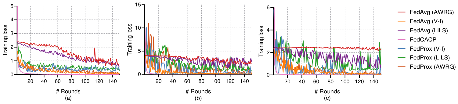
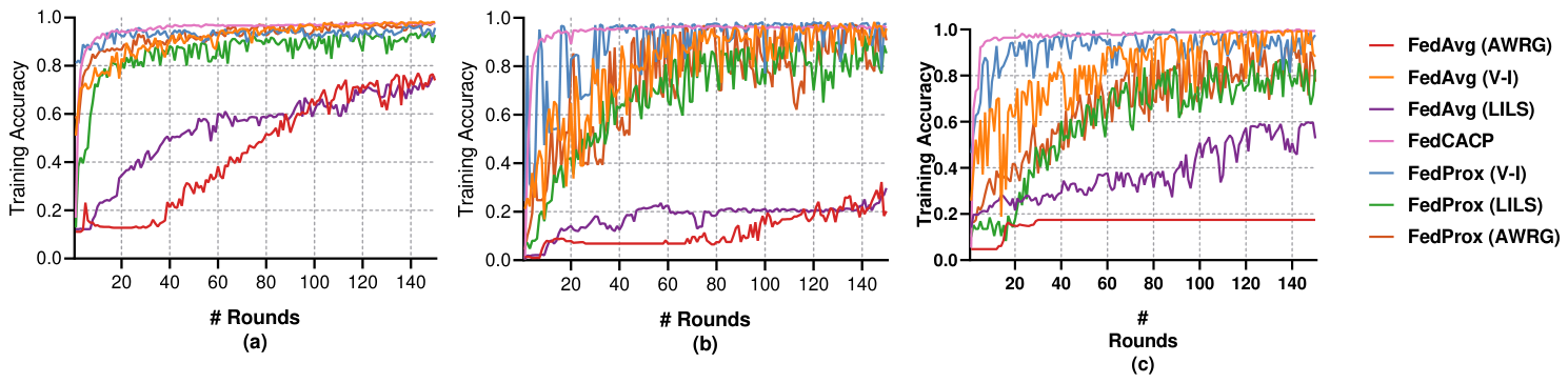
Figure 9 and Figure 10 present the training loss and training accuracy curves in Case 3, respectively. In both figures, subfigures (a), (b), and (c) correspond to the PLAID, WHITED, and COOLL datasets, respectively. Notably, FedCACP achieved the best performance on WHITED and COOLL, with F1-macro scores of 94.5% and 97.3%, respectively, and remained highly competitive on PLAID, with a F1-macro of 94.1%. Its strong overall performance and relatively low variance demonstrate the effectiveness of the context-aware conditional policy and feature alignment mechanism in handling complex client heterogeneity. Compared with most baselines, FedCACP provides a better trade-off among accuracy, F1-macro, and stability, confirming its robustness across challenging real-world scenarios.

5.5. Results in Case 4 (LoHoCV)

Table 6. Experimental results in Case 4 (LoHoCV) on the PLAID dataset.

Method	Accuracy	Precision	Recall	F1-Macro
Central (LILS)	80.4 ± 4.7	80.3 ± 4.4	80.4 ± 3.6	78.8 ± 3.6
Central (V-I)	75.6 ± 2.8	72.0 ± 4.5	70.9 ± 3.9	69.9 ± 4.1
Central (AWRG)	77.6 ± 4.7	77.1 ± 4.3	75.4 ± 5.2	74.1 ± 4.8
FedAvg (LILS)	75.3 ± 3.6	73.8 ± 5.7	70.5 ± 3.1	71.2 ± 4.2
FedAvg (V-I)	75.3 ± 1.5	72.6 ± 3.6	71.3 ± 0.6	71.1 ± 1.7
FedAvg (AWRG)	74.6 ± 1.7	71.7 ± 2.0	70.4 ± 1.4	70.2 ± 1.5
FedProx (LILS)	22.0 ± 5.3	13.7 ± 2.8	20.4 ± 0.9	13.1 ± 1.8
FedProx (V-I)	75.4 ± 2.4	69.3 ± 1.5	66.6 ± 3.5	64.9 ± 2.5
FedProx (AWRG)	81.1 ± 2.0	79.3 ± 2.6	76.5 ± 1.9	74.9 ± 2.0
FedCACP	80.3 ± 2.0	80.4 ± 0.6	80.2 ± 1.5	79.7 ± 2.5

Note: LoHoCV denotes leave-one-house-out cross-validation.

reports the results for Case 4, which adopts a leave-one-house-out cross-validation setting to evaluate generalization to unseen houses. Among the centralized methods, LILS achieved the best performance, with $80.4\pm 4.7\%$ accuracy and $78.8\pm 3.6\%$ F1-macro. Although V-I and AWRG representations also yielded decent results, their generalization ability was generally inferior to LILS in this setting.

For federated methods, performance varies significantly depending on the feature representation. FedAvg maintains relatively consistent accuracy across all variants, but its F1-macro remains moderate, suggesting limited adaptability. FedProx, on the other hand, exhibits large performance fluctuations. When combined with LILS, it performs extremely poorly, with only $22.0\pm 5.3\%$ accuracy and $13.1\pm 1.8\%$ F1-macro. In contrast, with AWRG features, FedProx reaches $81.1\pm 2.0\%$ accuracy and $74.9\pm 2.0\%$ F1-macro. A possible explanation is that LILS learns its feature representation jointly with model training, whereas V-I trajectory and AWRG use fixed representations generated before federated optimization. Under the leave-one-house-out setting, client-specific appliance signatures may lead to inconsistent local LILS representations across clients. In addition, the proximal term in FedProx may restrict local adaptation, causing FedProx (LILS) to converge numerically but reach a suboptimal representation space. In contrast, fixed V-I and AWRG representations decouple feature construction from federated training and, therefore, show more stable performance. The proposed FedCACP method achieves the most competitive F1-macro among the federated approaches, reaching $80.3\pm 2.0\%$ accuracy and $79.7\pm 2.5\%$ F1-macro. This indicates that FedCACP provides robust generalization to unseen houses while avoiding the severe degradation observed in some FedProx variants.

5.6. Effect of the Number of Clients K

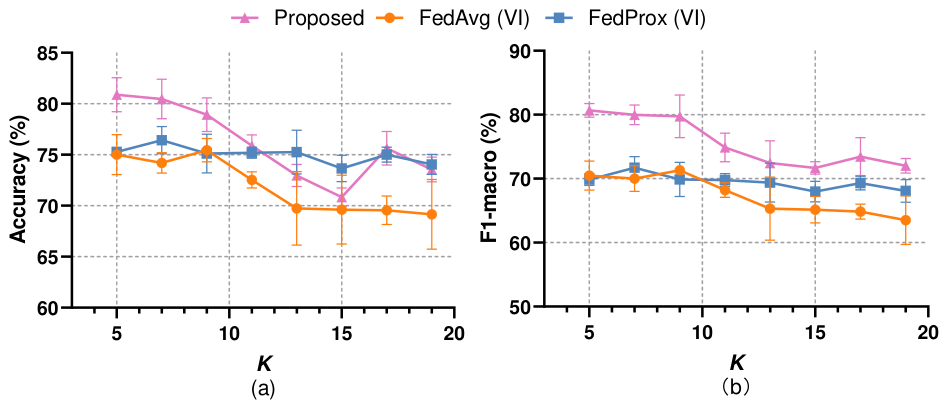
We now examine how the number of clients K affects performance. As shown in Figure 11, increasing K from 5 to 19 leads to performance degradation for all methods due to increased data fragmentation. FedAvg (V-I) is most affected, with nearly a 6% drop in accuracy, over 7% reduction in F1-macro, and a 74% increase in variance. FedProx (V-I) shows stronger robustness, maintaining accuracy above 73.6% and experiencing 38% less F1-macro degradation than FedAvg, although its F1-macro remains below 71.7%.

The proposed method consistently outperforms the baselines across all K. It starts with 80.9% accuracy and 80.7% F1-macro at $K=5$, and still retains 73.6% accuracy and 72.0% F1-macro at $K=19$. Its relatively low variance also indicates more stable generalization as client heterogeneity increases.

5.7. Privacy Discussion

We analyzed the privacy property of FedCACP from the perspective of information exposure. We considered an honest-but-curious server that follows the training protocol but may inspect the uploaded parameters. For client k at communication round t, the information observable by the server is $\left\{{\mathit{W}}_k^{f,\left(t\right)},{\widehat{\mathit{W}}}_k^{h,\left(t\right)},{\mathit{W}}_k^{a,\left(t\right)}\right\}$. In contrast, the private local dataset ${\mathcal{D}}_k={\left\{({\mathbf{x}}_i^k,y_i^k)\right\}}_{i=1}^{n_k}$ is never transmitted. Therefore, the server does not directly observe original samples.

The personalized routing variables are also generated locally. Specifically, for a local sample ${\mathbf{x}}_i$, FedCACP computes ${\mathit{h}}_i={\mathcal{F}}_k({\mathbf{x}}_i;{\mathit{W}}_k^f),{\mathit{z}}_i=\left({\displaystyle \frac{{\mathit{v}}_k}{\parallel {\mathit{v}}_k{\parallel }_2}}\right)\odot {\mathit{h}}_i,({\mathit{r}}_i,{\mathit{s}}_i)={\mathcal{A}}_k({\mathit{z}}_i;{\mathit{W}}_k^a).$ Although the server receives the uploaded model parameters, it does not have access to the input ${\mathbf{x}}_i$. Thus, it cannot directly compute the true feature ${\mathit{h}}_i$, fused representation ${\mathit{z}}_i$, or gating policies $({\mathit{r}}_i,{\mathit{s}}_i)$ for the local training samples. In this sense, FedCACP keeps personalized routing behavior on the client side.

For the uploaded head, FedCACP uses the interpolated parameter ${\widehat{\mathit{W}}}_k^{h,\left(t\right)}=\delta {\mathit{W}}_k^{h,\left(t\right)}+(1-\delta ){\mathit{W}}^{h,\left(t\right)}$. This interpolation regularizes the uploaded head toward the global head, since ${\widehat{\mathit{W}}}_k^{h,\left(t\right)}-{\mathit{W}}^{h,\left(t\right)}=\delta \left({\mathit{W}}_k^{h,\left(t\right)}-{\mathit{W}}^{h,\left(t\right)}\right)$. Therefore, the deviation of the uploaded head from the global head is scaled by $\delta$. Nevertheless, a server that knows $\delta$ and ${\mathit{W}}^{h,\left(t\right)}$ may still infer ${\mathit{W}}_k^{h,\left(t\right)}$ from ${\widehat{\mathit{W}}}_k^{h,\left(t\right)}$ when $\delta >0$. Therefore, FedCACP should be regarded as a privacy-aware FL framework that reduces raw-data and sample-level behavior exposure, rather than a method with formal privacy guarantees.

5.8. Computational Cost Discussion

Table 7. Computation time and communication cost on the PLAID dataset under Case 3.

Methods	Computation			Communication
	Rounds to Conv.	Time/Round (s)	Total Time (s)	Comm./Round (MB)	Total Comm. (MB)
FedAvg (V-I)	$131.8\pm 17.6$	$0.124\pm 0.007$	$16.30\pm 1.68$	$15.37\pm 0.00$	$2025.40\pm 270.00$
FedProx (V-I)	$130.0\pm 21.7$	$8.032\pm 0.331$	$1042.95\pm 169.91$	$15.37\pm 0.00$	$1997.74\pm 332.80$
FedCACP	$35.4\pm 15.9$	$1.038\pm 0.251$	$35.48\pm 14.33$	$33.53\pm 0.00$	$1187.07\pm 531.58$

Note: The communication cost is calculated based on the transmitted model parameters. For FedAvg (V-I) and FedProx (V-I), the per-round transmitted parameters are estimated as $2{\sum }_{k=1}^K\left(\left|{\mathit{W}}_k^f\right|+\left|{\mathit{W}}_k^h\right|\right)$, where the factor 2 accounts for both server-to-client downloads and client-to-server uploads. For FedCACP, the transmitted parameters are estimated as $2{\sum }_{k=1}^K\left(\left|{\mathit{W}}_k^f\right|+\left|{\widehat{\mathit{W}}}_k^h\right|+\left|{\mathit{W}}_k^a\right|\right)$. Each parameter is stored as a 32-bit floating-point value and converted to MB.

compares the computation time and communication cost of FedAvg (V-I), FedProx (V-I), and FedCACP on the PLAID dataset under Case 3. For a fair comparison, all methods are evaluated with $K=5$ clients and full client participation in each communication round.

Compared with FedAvg (V-I) and FedProx (V-I), FedCACP requires a larger communication cost per round. This is because FedCACP transmits additional personalized components, including the feature extractor, the interpolated head, and the CACP module. Specifically, clients upload $\{{\mathit{W}}_k^f,{\widehat{\mathit{W}}}_k^h,{\mathit{W}}_k^a\}$, whereas FedAvg and FedProx transmit the standard model parameters. As a result, the communication cost per round of FedCACP is 33.53 MB, which is higher than the 15.37 MB of FedAvg (V-I) and FedProx (V-I). Nevertheless, FedCACP converges in fewer communication rounds. As shown in Table 7, FedCACP requires only $35.4\pm 15.9$ rounds to convergence, while FedAvg (V-I) and FedProx (V-I) require $131.8\pm 17.6$ and $130.0\pm 21.7$ rounds, respectively. Therefore, although FedCACP has a higher per-round communication cost, its total communication cost is reduced to $1187.07\pm 531.58$ MB.

In terms of computation time, FedCACP requires more time per round than FedAvg (V-I) due to the additional personalized and context-aware computations introduced by the CACP module. This indicates that the performance improvement and reduced communication rounds are obtained at the cost of extra local computation. However, CACP is designed as an auxiliary policy module rather than an additional convolutional backbone, and the main computational cost still comes from the feature extractor. Therefore, the additional overhead is moderate in the current experimental setting. For resource-constrained smart-meter nodes, this trade-off should be carefully considered, and lightweight CACP designs, pruning, quantization, and hardware-aware optimization will be investigated in future work.

Frequent cloud–edge communication may increase bandwidth usage and energy consumption in practical smart-meter edge deployments. Table 7 therefore reports the communication cost of each method, including both server-to-client downloads and client-to-server uploads. Since this study does not directly measure energy consumption on physical smart-meter edge nodes, hardware-based energy evaluation is left for future work.

6. Conclusions

This paper proposes a personalized FL method for appliance recognition in NILM that addresses two key challenges: privacy-preserving collaborative training without raw data exchange, and performance degradation due to inter-client label distribution skew. Each client maintains both personalized and global model components, coordinated by a context-aware conditional policy module that adaptively controls information sharing through learnable gating mechanisms. Extensive experiments on real-world datasets demonstrate competitive and stable performance compared with federated baselines. Specifically, the method maintains accuracy above $93.6\%$ on PLAID across Dirichlet skew levels ($\alpha =0.01$ to $0.1$). In the leave-one-house-out evaluation on PLAID, it achieves $80.3\pm 2.0\%$, and on WHITED under house-based splits, it reaches $95.9\pm 1.6\%$. These results validate the method’s effectiveness across diverse and challenging non-IID scenarios.

Limitations and Future Work: One limitation is that FedCACP currently assumes that all clients use the same network architecture, which enables direct parameter aggregation at the server. This may limit its deployment in heterogeneous-device scenarios where clients have different computational resources, memory budgets, or sensing configurations. Future work will extend FedCACP to model-heterogeneous federated learning—for example, by using shared representation interfaces, knowledge distillation, or prototype aggregation. Another limitation is that the house-partitioned settings of WHITED and COOLL rely on artificially constructed virtual houses due to the lack of real household metadata, which may not fully reflect real household-level distribution shifts. Finally, since the current experiments are based mainly on normal operating conditions, future work will incorporate human-centered load behavior and resilience-aware constraints for extreme-event scenarios.

References

1. Hart, G.W. Nonintrusive appliance load monitoring. Proc. IEEE 1992, 80, 1870–1891. [Google Scholar] [CrossRef] [Scilit]
2. Fan, P.; Li, S.; Bu, S.; Wen, Y.; Chung, C.Y. Resilient Power Systems against Wildfire Risks: Towards a Human-Centric and Secure Future. CSEE J. Power Energy Syst. 2025, 11, 2553–2575. [Google Scholar] [CrossRef] [Scilit]
3. Fan, P.; Bu, S.; Li, S.; Fang, S.; Zhang, C.; Ke, S. Resilience enhancement strategy for multi-microgrids with electric vehicle under extreme weather conditions. CSEE J. Power Energy Syst. 2026, 1–12, Early Access. [Google Scholar] [CrossRef]
4. Chen, J.; Wang, X.; Zhang, X.; Zhang, W. Temporal and spectral feature learning with two-stream convolutional neural networks for appliance recognition in NILM. IEEE Trans. Smart Grid 2021, 13, 762–772. [Google Scholar] [CrossRef] [Scilit]
5. Makonin, S.; Popowich, F.; Bajić, I.V.; Gill, B.; Bartram, L. Exploiting HMM Sparsity to Perform Online Real-Time Nonintrusive Load Monitoring. IEEE Trans. Smart Grid 2016, 7, 2575–2585. [Google Scholar] [CrossRef] [Scilit]
6. Balletti, M.; Piccialli, V.; Sudoso, A.M. Mixed-integer nonlinear programming for state-based non-intrusive load monitoring. IEEE Trans. Smart Grid 2022, 13, 3301–3314. [Google Scholar] [CrossRef] [Scilit]
7. Zhang, C.; Zhong, M.; Wang, Z.; Goddard, N.; Sutton, C. Sequence-to-Point Learning with Neural Networks for Non-Intrusive Load Monitoring. Proc. AAAI Conf. Artif. Intell. 2018, 32, 2604–2611. [Google Scholar] [CrossRef] [Scilit]
8. De Baets, L.; Dhaene, T.; Deschrijver, D.; Develder, C.; Berges, M. VI-based appliance classification using aggregated power consumption data. In Proceedings of the 2018 IEEE International Conference on Smart Computing (SMARTCOMP), Taormina, Italy, 18–20 June 2018; IEEE: New York, NY, USA, 2018; pp. 179–186. [Google Scholar]
9. Gao, J.; Kara, E.C.; Giri, S.; Bergés, M. A feasibility study of automated plug-load identification from high-frequency measurements. In Proceedings of the 2015 IEEE Global Conference on Signal and Information Processing (GlobalSIP), Orlando, FL, USA, 14–16 December 2015; IEEE: New York, NY, USA, 2015; pp. 220–224. [Google Scholar]
10. De Baets, L.; Ruyssinck, J.; Develder, C.; Dhaene, T.; Deschrijver, D. Appliance classification using VI trajectories and convolutional neural networks. Energy Build. 2018, 158, 32–36. [Google Scholar] [CrossRef] [Scilit]
11. Paul, S.; Upadhyay, N.; Padhy, N.P. Residential appliance identification using 1-D convolutional neural network based on multiscale sinusoidal initializers. IEEE Trans. Ind. Inform. 2022, 18, 7444–7453. [Google Scholar] [CrossRef] [Scilit]
12. Pan, X.; Ye, L.; Weng, D.; Chen, J.; Yin, J. RTNILM: A Deep Robust Transfer Neural Network for Practical Application of NILM. IEEE Trans. Ind. Inform. 2025, 21, 6968–6978. [Google Scholar] [CrossRef] [Scilit]
13. Liu, Y.; Wang, X.; You, W. Non-intrusive load monitoring by voltage–current trajectory enabled transfer learning. IEEE Trans. Smart Grid 2018, 10, 5609–5619. [Google Scholar]
14. Tabanelli, E.; Brunelli, D.; Acquaviva, A.; Benini, L. Trimming feature extraction and inference for MCU-based edge NILM: A systematic approach. IEEE Trans. Ind. Inform. 2021, 18, 943–952. [Google Scholar] [CrossRef] [Scilit]
15. Liu, Y.; Xu, Q.; Yang, Y.; Zhang, W. Detection of electric bicycle indoor charging for electrical safety: A nilm approach. IEEE Trans. Smart Grid 2023, 14, 3862–3875. [Google Scholar] [CrossRef] [Scilit]
16. Li, Q.; Ye, J.; Song, W.; Tse, Z. Energy disaggregation with federated and transfer learning. In Proceedings of the 2021 IEEE 7th World Forum on Internet of Things (WF-IoT), New Orleans, LA, USA, 14 June 2021–31 July 2021; IEEE: New York, NY, USA, 2021; pp. 698–703. [Google Scholar]
17. Pötter, H.; Lee, S.; Mossé, D. Towards Privacy-preserving Framework for Non-Intrusive Load Monitoring. In Proceedings of the Twelfth ACM International Conference on Future Energy Systems, New York, NY, USA, 28 June 2021–2 July 2021; e-Energy ’21. pp. 259–263. [Google Scholar]
18. Dai, S.; Meng, F.; Wang, Q.; Chen, X. FederatedNILM: A Distributed and Privacy-Preserving Framework for Non-Intrusive Load Monitoring Based on Federated Deep Learning. In Proceedings of the 2023 International Joint Conference on Neural Networks (IJCNN), Gold Coast, Australia, 18–23 June 2023; pp. 1–8. [Google Scholar] [CrossRef] [Scilit]
19. Tan, A.Z.; Yu, H.; Cui, L.; Yang, Q. Towards personalized federated learning. IEEE Trans. Neural Netw. Learn. Syst. 2022, 34, 9587–9603. [Google Scholar] [CrossRef] [Scilit]
20. Wang, H.; Si, C.; Liu, G.; Zhao, J.; Wen, F.; Xue, Y. Fed-NILM: A federated learning-based non-intrusive load monitoring method for privacy-protection. Energy Convers. Econ. 2022, 3, 51–60. [Google Scholar] [CrossRef] [Scilit]
21. McMahan, B.; Moore, E.; Ramage, D.; Hampson, S.; y Arcas, B.A. Communication-efficient learning of deep networks from decentralized data. In Proceedings of the Artificial Intelligence and Statistics, Fort Lauderdale, FL, USA, 20–22 April 2017; PMLR, 2017. pp. 1273–1282. [Google Scholar]
22. Wang, X.; Li, W. Mtfed-nilm: Multi-task federated learning for non-intrusive load monitoring. In Proceedings of the 2022 IEEE Intl Conf on Dependable, Autonomic and Secure Computing, Intl Conf on Pervasive Intelligence and Computing, Intl Conf on Cloud and Big Data Computing, Intl Conf on Cyber Science and Technology Congress (DASC/PiCom/CBDCom/CyberSciTech), Falerna, Italy, 12–15 September 2022; IEEE: New York, NY, USA, 2022; pp. 1–8. [Google Scholar]
23. Dai, S.; Meng, F.; Wang, Q.; Chen, X. DP2-NILM: A distributed and privacy-preserving framework for non-intrusive load monitoring. Renew. Sustain. Energy Rev. 2024, 191, 114091. [Google Scholar] [CrossRef] [Scilit]
24. Chang, X.; Li, W.; Zomaya, A.Y. Fed-GBM: A cost-effective federated gradient boosting tree for non-intrusive load monitoring. In Proceedings of the Thirteenth ACM International Conference on Future Energy Systems, Virtual Event, 28 June–1 July 2022; pp. 63–75. [Google Scholar]
25. Pan, Z.; Wang, H.; Li, C.; Wang, H.; Zhao, J. Perfednilm: A practical personalized federated learning-based non-intrusive load monitoring. Ind. Artif. Intell. 2024, 2, 4. [Google Scholar] [CrossRef] [Scilit]
26. Agarwal, V.; Ardakanian, O.; Pal, S. A Robust and Privacy-Aware Federated Learning Framework for Non-Intrusive Load Monitoring. IEEE Trans. Sustain. Comput. 2024, 9, 766–777. [Google Scholar] [CrossRef] [Scilit]
27. Li, Y.; Yao, R.; Qin, D.; Wang, Y. Lightweight Federated Learning for On-Device Non-Intrusive Load Monitoring. IEEE Trans. Smart Grid 2025, 16, 1950–1961. [Google Scholar] [CrossRef] [Scilit]
28. Wang, T.; Dong, Z. Blockchain-Based Clustered Federated Learning for Non-Intrusive Load Monitoring. IEEE Trans. Smart Grid 2024, 15, 2348–2361. [Google Scholar] [CrossRef] [Scilit]
29. Bousbiat, H.; Himeur, Y.; Varlamis, I.; Bensaali, F.; Amira, A. Neural Load Disaggregation: Meta-Analysis, Federated Learning and Beyond. Energies 2023, 16, 991. [Google Scholar] [CrossRef] [Scilit]
30. Du, L.; He, D.; Harley, R.G.; Habetler, T.G. Electric load classification by binary voltage–current trajectory mapping. IEEE Trans. Smart Grid 2015, 7, 358–365. [Google Scholar] [CrossRef] [Scilit]
31. Faustine, A.; Pereira, L.; Klemenjak, C. Adaptive weighted recurrence graphs for appliance recognition in non-intrusive load monitoring. IEEE Trans. Smart Grid 2020, 12, 398–406. [Google Scholar] [CrossRef] [Scilit]
32. Sun, B.; Saenko, K. Deep coral: Correlation alignment for deep domain adaptation. In Proceedings of the Computer Vision–ECCV 2016 Workshops, Amsterdam, The Netherlands, 8–10 and 15–16 October 2016; proceedings, part III 14; Springer: Cham, Switzerland, 2016; pp. 443–450. [Google Scholar]
33. Bengio, E.; Bacon, P.L.; Pineau, J.; Precup, D. Conditional computation in neural networks for faster models. arXiv 2015, arXiv:1511.06297. [Google Scholar]
34. Jang, E.; Gu, S.; Poole, B. Categorical reparameterization with gumbel-softmax. arXiv 2016, arXiv:1611.01144. [Google Scholar]
35. Zhang, J.; Hua, Y.; Wang, H.; Song, T.; Xue, Z.; Ma, R.; Guan, H. Fedcp: Separating feature information for personalized federated learning via conditional policy. In Proceedings of the 29th ACM SIGKDD Conference on Knowledge Discovery and Data Mining, Long Beach, CA, USA, 6–10 August 2023; pp. 3249–3261. [Google Scholar]
36. Yi, L.; Wang, G.; Liu, X.; Shi, Z.; Yu, H. Fedgh: Heterogeneous federated learning with generalized global header. In Proceedings of the 31st ACM International Conference on Multimedia, Ottawa, ON, Canada, 29 October–3 November 2023; pp. 8686–8696. [Google Scholar]
37. Guo, Y.; Shi, H.; Kumar, A.; Grauman, K.; Rosing, T.; Feris, R. Spottune: Transfer learning through adaptive fine-tuning. In Proceedings of the IEEE/CVF Conference on Computer Vision and Pattern Recognition, Long Beach, CA, USA, 16–17 June 2019; pp. 4805–4814. [Google Scholar]
38. Gao, J.; Giri, S.; Kara, E.C.; Bergés, M. Plaid: A public dataset of high-resoultion electrical appliance measurements for load identification research: Demo abstract. In Proceedings of the 1st ACM Conference on Embedded Systems for Energy-Efficient Buildings, Memphis, TN, USA, 3–6 November 2014; pp. 198–199. [Google Scholar]
39. Kahl, M.; Haq, A.U.; Kriechbaumer, T.; Jacobsen, H.A. Whited-a worldwide household and industry transient energy data set. In Proceedings of the 3rd International Workshop on Non-Intrusive Load Monitoring, Vancouver, BC, Canada, 14–15 May 2016; pp. 1–4. [Google Scholar]
40. Picon, T.; Meziane, M.N.; Ravier, P.; Lamarque, G.; Novello, C.; Bunetel, J.C.L.; Raingeaud, Y. COOLL: Controlled on/off loads library, a public dataset of high-sampled electrical signals for appliance identification. arXiv 2016, arXiv:1611.05803. [Google Scholar]
41. Zhang, Y.; Wu, H.; Ma, Q.; Yang, Q.; Wang, Y. A learnable image-based load signature construction approach in NILM for appliances identification. IEEE Trans. Smart Grid 2023, 14, 3841–3849. [Google Scholar] [CrossRef] [Scilit]
42. Li, T.; Sahu, A.K.; Zaheer, M.; Sanjabi, M.; Talwalkar, A.; Smith, V. Federated optimization in heterogeneous networks. Proc. Mach. Learn. Syst. 2020, 2, 429–450. [Google Scholar]
43. Han, Y.; Gao, Q.; Chen, H.; Zhao, Q. A Few-Shot Learning method for Non-Intrusive Load Monitoring with VI Trajectory Features. IEEE Sens. J. 2024, 24, 11867–11877. [Google Scholar] [CrossRef] [Scilit]
Figure 1. Overview of the typical federated learning process.
Energies 19 03445 g001
Figure 2. Illustration of the feature extractor and prediction head. Conv and FC denote convolutional layer and fully connected layer, respectively.
Energies 19 03445 g002
Figure 3. Example of transforming voltage–current waveforms into HSV trajectory images. (a) Voltage waveform; (b) current waveform; (c) V-I trajectory; (d) HSV-encoded trajectory image visualized in RGB (Red, green, blue) format. The colors represent the encoded HSV values of the trajectory points.
Energies 19 03445 g003
Figure 4. Local training process and parameter update strategy in FedCACP.
Energies 19 03445 g004
Figure 5. Proposed neural network architecture.
Energies 19 03445 g005
Figure 6. Class distributions across 5 clients on the PLAID dataset generated by Dirichlet partitioning with (a) α = 0.01 , (b) α = 0.1 , and (c) α = 1.0 . The circle size indicates the number of samples.
Energies 19 03445 g006
Figure 7. Impact of δ on performance.
Energies 19 03445 g007
Figure 8. Training dynamics under Dirichlet-based non-IID settings. (a) Training loss with α = 1.0 ; (b) training loss with α = 0.1 ; (c) training loss with α = 0.01 ; (d) accuracy with α = 1.0 ; (e) accuracy with α = 0.1 ; (f) accuracy with α = 0.01 .
Energies 19 03445 g008
Figure 9. Training loss in Case 3. (a) PLAID dataset; (b) WHITED dataset; (c) COOLL dataset.
Energies 19 03445 g009
Figure 10. Training accuracy in Case 3. (a) PLAID dataset; (b) WHITED dataset; (c) COOLL dataset.
Energies 19 03445 g010
Figure 11. The averaged test accuracy (%) and F1-macro (%) under Case 4 with different K. (a) Average test accuracy; (b) average F1-macro.
Energies 19 03445 g011