Transformer–Customer Relationship Identification Using Hyperparameter-Optimized t-Distributed Stochastic Neighbor Embedding and Gaussian Mixture Clustering

Abstract

The transformer–customer relationship is essential for the operation and management of low-voltage distribution systems. However, manual registration and verification of transformer–customer relationships are costly and prone to mismatches due to delayed archival updates. To address this issue, this paper proposes a data-driven method for transformer–customer relationship identification using smart meter voltage measurements. Specifically, raw voltage data obtained from Advanced Metering Infrastructure (AMI) are embedded into a low-dimensional feature space using t-distributed stochastic neighbor embedding (t-SNE). The key parameters of t-SNE are adaptively optimized using the proposed Dream Optimization Algorithm–Whale Optimization Algorithm (DOA-WOA), with the silhouette coefficient serving as the objective function. Subsequently, a Gaussian Mixture Model is applied to cluster the samples in the obtained low-dimensional feature space for transformer–customer relationship identification. The simulation results verify the effectiveness and robustness of the proposed method under different missing data rates and voltage measurement errors. Experiments conducted on real low-voltage distribution transformer datasets and incomplete data scenarios demonstrate that the proposed method achieves identification accuracies of 98.4% and 96.8%, respectively.

1. Introduction

The transformer–customer relationship is fundamental information for the operation and management of low-voltage distribution systems (LVDSs) [1]. However, manual registration and maintenance processes are prone to mismatches and update delays in practical engineering applications [2]. Incorrect transformer–customer relationships may adversely affect applications such as line loss analysis, fault location, and three-phase imbalance mitigation [3]. Therefore, accurate transformer–customer relationship identification is critical for the secure and intelligent operation of LVDSs [4].

In recent years, AMI has been widely deployed in LVDSs [5,6,7]. Meanwhile, the integration of distributed energy resources and electric vehicles has made network operation increasingly dynamic. These changes require more accurate and up-to-date transformer–customer relationship information. However, manual maintenance of customer archives is difficult and often fails to keep pace with network changes. Consequently, data-driven identification based on AMI measurements has become an important means of updating and verifying transformer–customer relationships.

Conventional approaches for customer–transformer relationship identification mainly rely on field inspection and power line carrier-based devices [8]. Field inspection is inefficient, whereas power line carrier-based methods require additional equipment and are susceptible to communication noise [9]. Current data-driven studies can generally be classified into three categories. The first category consists of methods based on power or current conservation, where the identification problem is formulated as solving the energy balance between customers and transformers. Zhao et al. [10] incorporated the aggregated power conservation relationship between the transformer side and the customer side into a model to achieve identification and verification. Hu et al. [11] jointly optimized voltage clustering quality indices with power-balance-based line loss and power loss coefficients for transformer–customer relationship identification. Liu et al. [12] developed a physics-informed neural network incorporating power flow mechanisms into low-voltage secondary-side modeling for identification. These approaches typically require complete and high-quality real-time measurements, making them sensitive to data availability and accuracy. The second category models transformer–customer relationship identification as a classification problem, learning voltage or current temporal features to enable identification. Ni et al. [13] proposed an end-to-end deep temporal clustering framework that integrates convolutional temporal representation learning with a clustering layer for low-voltage network topology identification. Huang et al. [14] constructed a deep feature extraction network combined with deep Gaussian mixture clustering and introduced an adaptive cluster structure mechanism to identify transformer–customer relationships in low-voltage systems. Tang et al. [15] developed an LSTM–GCN hybrid network that extracts temporal features from voltage and power data and captures dependencies among nodes, enabling topology identification. Nevertheless, neural network training generally requires large-scale datasets, leading to high implementation costs and long training cycles, and may suffer from limited generalization capability. The third category is based on voltage or power time-series similarity analysis combined with clustering techniques. Al Khafaf et al. [16] formulated transformer–customer relationship identification as an unsupervised clustering problem based on voltage time-series similarity, using real AMI data to achieve transformer–customer identification without prior labels. Lei et al. [17] proposed a two-stage identification framework: voltage time-series similarity features are first constructed and an improved K-means algorithm is applied for preliminary grouping, followed by graph-structure-based refinement. Li et al. [18] developed customer feature profiling based on voltage and power time-series, and employed temporal similarity metrics and clustering methods to achieve transformer–customer relationship identification. Representative transformer–customer relationship identification methods are summarized in

Table 1. Advantages and limitations of identification methods.

Category	Methods	Advantages	Limitations
Power/current conservation	[10,11,12]	Strong physical interpretability	Sensitive to measurement completeness and accuracy
Deep learning	[13,14,15]	Automatic feature extraction	Large data demand, limited generalization
Similarity-based clustering	[16,17,18]	No labeled data required, simple implementation	Sensitive to feature quality and parameter settings

, together with their main advantages and limitations. Despite recent progress, transformer–customer relationship identification is still not fully resolved. AMI data often contain missing values and measurement noise. Customers supplied by different transformers may exhibit similar voltage patterns. These factors reduce the reliability of similarity analysis. In addition, the performance of many dimensionality reduction methods depends on manually selected parameters. Therefore, a robust and adaptive identification method is still needed.

Considering the nonlinear characteristics of customer voltage data and the sensitivity of t-SNE to hyperparameter settings, t-SNE is adopted to extract discriminative low-dimensional representations, while the DOA-WOA is employed to adaptively optimize its key hyperparameters. Subsequently, a Gaussian Mixture Model is utilized to identify transformer–customer relationships due to its capability of modeling clusters with different distributions. Major contributions of this paper are summarized below:

(1)

A data-driven transformer–customer relationship identification framework is developed. By exploiting the similarity characteristics of customer voltage measurements within the same transformer area, the mapping relationship between low-voltage customers and distribution transformers can be identified without requiring network topology information.

(2)

A hybrid parameter optimization strategy for t-SNE is proposed. To address the sensitivity of t-SNE to hyperparameters, a hybrid optimization algorithm that integrates the exploration capability of the Dream Optimization Algorithm and the exploitation ability of the Whale Optimization Algorithm is designed to automatically search for suitable dimensionality-reduction parameters.

(3)

An identification method integrating optimized t-SNE and a Gaussian Mixture Model is established. Optimized t-SNE is employed to obtain low-dimensional feature representations of customer voltage profiles, and a Gaussian Mixture Model is then applied to perform probabilistic clustering, enabling accurate identification of customer groups corresponding to different distribution transformers.

2. Issue Statement and Framework

2.1. Issue Statement

Transformer–customer relationship identification aims to determine the actual mapping between each electricity customer and its supplying distribution transformer based on available measurement data. Given the voltage time-series collected from AMI and without relying on manually maintained customer archives, the objective is to automatically partition customers into groups corresponding to their supplying transformers. The identified groups should accurately reflect the physical topology of the LVDS while maintaining robustness against measurement noise, missing data, and parameter variations.

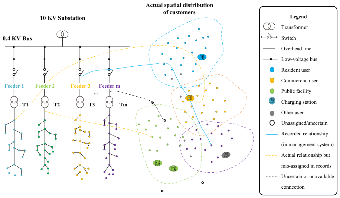
Figure 1 shows a practical transformer–customer relationship in a low-voltage distribution system, where multiple feeders are connected to the low-voltage bus and each transformer supplies a group of customers. Ideally, customers associated with the same transformer exhibit a clear spatial aggregation and consistent connection relationship. However, in actual operation, discrepancies often exist between the recorded and the real transformer–customer relationships. As shown in Figure 1, some customers are incorrectly assigned, some connections are uncertain or missing, and overlapping supply areas further complicate the association. These issues indicate that the transformer–customer relationship in practice is often inaccurate and incomplete, which poses significant challenges for reliable identification.

Considering these issues, a data-driven identification framework is required to capture nonlinear characteristics, adaptively optimize parameters, and maintain reliable performance under incomplete data conditions.

2.2. Framework of the Proposed Method

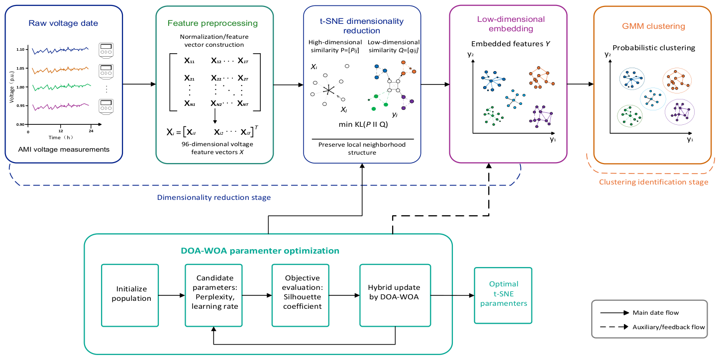
A transformer–customer relationship identification method is developed by integrating high-dimensional feature embedding with probabilistic clustering based on a Gaussian Mixture Model, as illustrated in Figure 2. Starting from multi-source data such as customer voltage measurements, high-dimensional features are constructed and then mapped into a low-dimensional space using t-SNE to capture the intrinsic data structure. To ensure high-quality embedding, the t-SNE parameters are adaptively optimized by an improved DOA-WOA formulated as an optimization problem. Finally, the data distribution is modeled using a GMM (Gaussian Mixture Model), and the transformer–customer relationships are identified based on the posterior probability distribution.

3. Proposed Transformer–Customer Identification Model

3.1. Dimensionality Reduction Based on Parameter-Optimized t-SNE

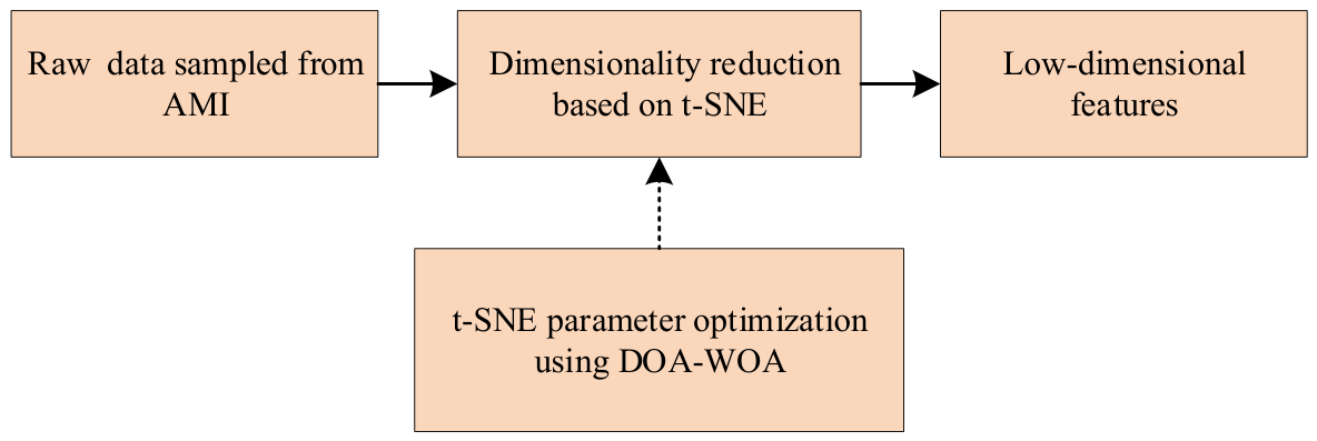
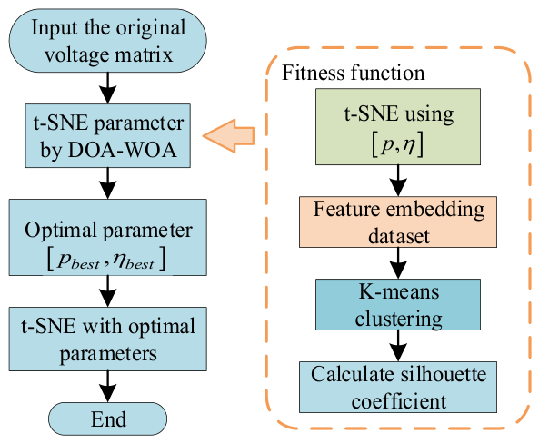
The customer voltage collected by AMI constitute high-dimensional time-series data, which usually contain fluctuation characteristics (peak-to-valley difference), temporal shape features (the timing of peaks and valleys and their variation trends), as well as inter-user voltage correlation. Therefore, it is necessary to perform dimensionality reduction on the time-series data, extract representative feature dimensions, and cluster the resulting feature data to identify different transformer–customer relationships. The flow chart of t-SNE dimensionality reduction based on parameter optimization is shown in Figure 3.

3.1.1. t-SNE

t-SNE is adopted to generate low-dimensional representations of customer voltage profiles while retaining their local similarity structure [19]. The voltage measurements of each customer over the observation period are organized into a high-dimensional feature vector. Since customers supplied by the same transformer generally exhibit similar voltage variation patterns, preserving these neighborhood relationships can enhance the separability of customer groups and provide suitable features for subsequent clustering.

For customer feature vectors ${\tilde{X}}_i$ and ${\tilde{X}}_j$, their neighborhood similarity in the original feature space is described by the conditional probability

$$p_{j|i}={\displaystyle \frac{\exp \left(-{‖{\tilde{X}}_i-{\tilde{X}}_j‖}^2/2{\sigma }_i^2\right)}{{\displaystyle {\sum }_{k\ne i}\exp \left(-{‖{\tilde{X}}_i-{\tilde{X}}_k‖}^2/2{\sigma }_i^2\right)}}},$$

(1)

where $p_{j|i}$ denotes the probability that customer $j$ is regarded as a neighbor of customer $i$, and ${\sigma }_i$ controls the neighborhood scale around ${\tilde{X}}_i$ The conditional probabilities in both directions are then combined to obtain the symmetric similarity $p_{ij}$.

Let $y_i$ and $y_j$ denote the embedded coordinates of customers $i$ and $j$, respectively. Their similarity after dimensionality reduction is calculated using

$$q_{ij}={\displaystyle \frac{{(1+{‖y_i-y_j‖}^2)}^{-1}}{{\displaystyle {\sum }_{k\ne l}{(1+{‖y_k-y_l‖}^2)}^{-1}}}},$$

(2)

where $q_{ij}$ represents the pairwise similarity in the embedded feature space. The low-dimensional coordinates are determined by minimizing the discrepancy between $p_{ij}$ and $q_{ij}$:

$$C={\displaystyle \sum _{i\ne j}{p}_{ij}\log \frac{p_{ij}}{q_{ij}}},$$

(3)

where $C$ is the Kullback–Leibler divergence between the two similarity distributions. Minimizing C places customers with comparable voltage trajectories closer together while separating customers with different voltage characteristics, thereby producing the feature representation used by the subsequent GMM clustering procedure.

3.1.2. Improved DOA-WOA for t-SNE Parameter Optimization

Perplexity ($p$) and learning rate ($\eta$) are two key hyperparameters that strongly influence the quality of low-dimensional embeddings, according to the original t-SNE formulation and subsequent studies on parameter sensitivity [19,20]. Perplexity determines the effective neighborhood size used to preserve local data structures, whereas the learning rate affects the convergence behavior of the optimization process. Both parameters directly influence the separability of the embedded features and the subsequent clustering performance. In contrast, other parameters, such as the number of iterations and early exaggeration, are generally assigned recommended default values in the MATLAB R2024b implementation and mainly affect optimization convergence rather than the final embedding quality. Therefore, only perplexity and learning rate are selected as the optimization variables in this study.

Grid search and random search are applicable to low-dimensional hyperparameter optimization. However, their performance depends on the predefined sampling strategy and search resolution. A coarse search may overlook high-quality parameter combinations, whereas a fine search significantly increases the number of evaluations. In contrast, the proposed DOA-WOA performs adaptive global exploration and local exploitation without exhaustive enumeration. Moreover, the proposed optimization framework can be readily extended to additional hyperparameters in future applications.

Based on the above considerations, the improved DOA-WOA is employed to adaptively optimize the perplexity and learning rate of t-SNE. The silhouette coefficient is adopted as the objective function to quantitatively evaluate the quality of the low-dimensional embedding [11], as it simultaneously measures intra-cluster compactness and inter-cluster separation. A higher silhouette coefficient value indicates a clearer cluster structure in the embedded space and guides the optimizer toward parameter combinations that are more favorable for subsequent clustering.

The silhouette coefficient reflects both the intra-cluster compactness and the inter-cluster separation of samples. Its value ranges from −1 to 1, where a larger value indicates a clearer clustering structure. The formula for calculating the silhouette coefficient is given as follows:

$$a\left(i\right)={\displaystyle \frac{1}{\left|C_{c_i}\right|-1}}{\displaystyle \sum _{\begin{array}{l}{y}_i\in C_{c_i}\\ j\ne i\end{array}}‖y_i-y_j‖},$$

(4)

$$b\left(i\right)=\underset{k\ne c_i}{\min }\left({\displaystyle \frac{1}{\left|C_k\right|}}{\displaystyle \sum _{y_i\in C_k}‖y_i-y_j‖}\right),$$

(5)

$$s\left(i\right)={\displaystyle \frac{b\left(i\right)-a\left(i\right)}{\max \left\{\left.a\left(i\right),b\left(i\right)\right\}\right.}},$$

(6)

where $a\left(i\right)$ denotes the intra-cluster average distance; $b\left(i\right)$ represents the minimum average distance to other clusters; and $s\left(i\right)$ is the silhouette coefficient for sample $y_i$.

The final objective function is as follows:

$$SC={\displaystyle \frac{1}{n}}{\displaystyle \sum _{i=1}^{n}s\left(i\right)},$$

(7)

where the silhouette coefficient represents the average value of the silhouette coefficients of all samples.

Accordingly, the parameter optimization problem can be expressed as:

$$\underset{\theta }{\max }=SC\left(\theta \right),$$

(8)

where $\theta$ denotes the set of t-SNE parameters ($p$ and $\eta$) to be optimized. It should be noted that, although the silhouette coefficient is computed based on clustering results, it is only used here as an indicator to evaluate the quality of the feature embedding, rather than being tied to a specific clustering model.

A hybrid optimization strategy is developed to solve the parameter optimization problem formulated. While the Whale Optimization Algorithm (WOA) [21] exhibits strong global exploration capability in the early search stages, the population gradually converges toward the optimal solution as iterations proceed, leading to a decline in population diversity and a tendency to fall into premature convergence. Conversely, the Dream Optimization Algorithm (DOA) [22] relies on stochastic perturbations for local search, which effectively refines the solution space, yet it lacks a global guidance mechanism, resulting in limited search efficiency and stability when used independently. An improved DOA-WOA optimization algorithm is proposed to address these limitations, avoiding local optima and enhancing solution accuracy. The specific modifications are introduced as follows:

To characterize the state of the population during the search process, a population diversity metric based on group statistical characteristics is introduced. At each iteration, the mean population vector is calculated as:

$${\overline{x}}^{(t)}={\displaystyle \frac{1}{N}}{\displaystyle \sum _{i=1}^N{x}_i^{(t)}},$$

(9)

on this basis, the population diversity indicator is defined as:

$$D(t)={\displaystyle \frac{1}{N}}{\displaystyle \sum _{i=1}^N\frac{‖x_i^{(t)}-{\overline{x}}^{(t)}‖}{\mathrm{ub}-\mathrm{lb}}},$$

(10)

where $N$ denotes the population size, and lb and ub represent the lower bound and upper bound of the search space, respectively. The metric is used to quantify the dispersion degree of individuals within the solution space, thereby reflecting the overall state of the current search stage.

An adaptive hybrid search strategy is constructed based on the variation in the population diversity indicator. When the population diversity remains high, it indicates that the search is still in the global exploration phase, and the global search update rule of the WOA is therefore employed. Once the population diversity decreases below a predefined threshold, it suggests that the population may be entering a region of local convergence. At this stage, the local stochastic search operator of the DOA is introduced to perform local refinement. The aforementioned adaptive hybrid update mechanism can be uniformly expressed as the following piecewise function:

$$x_i^{(t+1)}=\left\{\begin{array}{l}{x}^{*}-A\cdot \left|C\cdot X^{*}-X_i^{(t)}\right|,D(t)>D_{thr}\\ x_i^{(t)}+\lambda \cdot \mathcal{N}(0,I),D(t)\le D_{thr}\end{array}\right.,$$

(11)

where $D_{thr}\in \left[0.15,0.30\right]$. If $D(t)>D_{thr}$, the algorithm is in the global exploration phase and employs the WOA’s encircling prey strategy. Otherwise, it is in the local optimization state and utilizes the DOA’s local perturbation search.

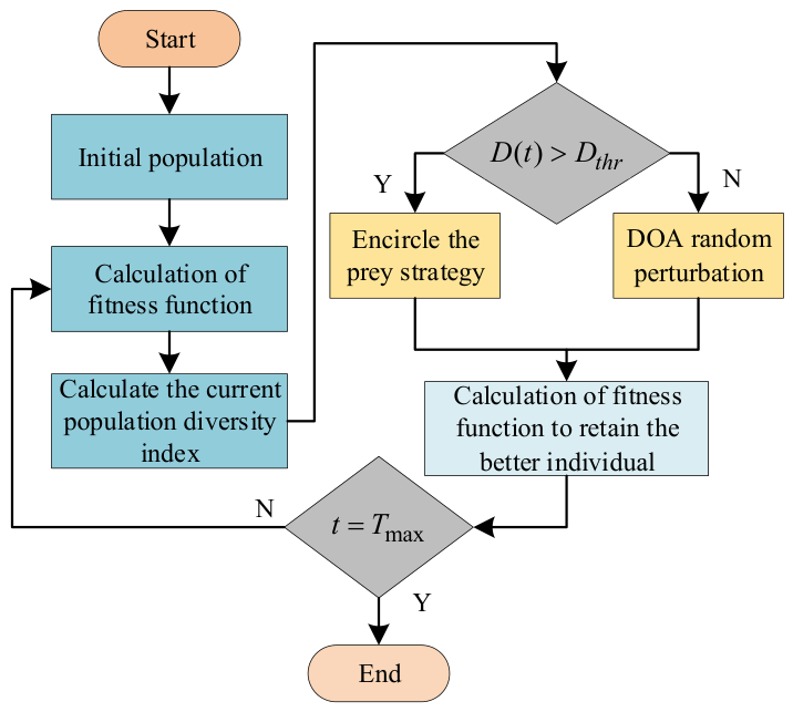
Figure 4 shows the flowchart of the DOA-WOA. After population initialization, the fitness and diversity index are evaluated at each iteration. The WOA update is activated when $D\left(t\right)>D_{thr}$; otherwise, DOA perturbation is used for local refinement. Candidate solutions are re-evaluated and the better individuals are retained until the prescribed iteration limit is reached, after which the best parameter pair is returned.

The improved DOA-WOA is employed to optimize the parameters of t-SNE. The flowchart of the DOA-WOA-based t-SNE parameter optimization is illustrated in Figure 5.

The selection of the DOA-WOA is motivated by the characteristics of the t-SNE hyperparameter optimization problem. Specifically, optimizing the perplexity and learning rate involves a nonlinear, multimodal, and gradient-free search space, making conventional gradient-based optimization methods unsuitable. The Dream Optimization Algorithm (DOA) provides strong global exploration capability by maintaining population diversity and reducing the risk of premature convergence, whereas the Whale Optimization Algorithm (WOA) offers efficient local exploitation through its adaptive encircling and spiral search mechanisms. By integrating these complementary search strategies, the proposed DOA-WOA achieves a better balance between exploration and exploitation, thereby improving the stability and convergence of the optimization process. Although other optimization techniques, such as Bayesian Optimization, Differential Evolution, CMA-ES, and Optuna-based frameworks, have also demonstrated effectiveness in hyperparameter optimization, they exhibit different optimization characteristics and computational trade-offs. In this study, DOA-WOA was selected because its population-based search mechanism is well suited to the highly nonlinear search landscape of t-SNE hyperparameter optimization while remaining straightforward to implement and independent of gradient information. The experimental results presented in Section 4 further demonstrate that the optimized t-SNE parameters obtained by the DOA-WOA lead to improved clustering performance and more discriminative low-dimensional feature representations for transformer–customer relationship identification.

3.1.3. Performance Analysis

Table 2. Six benchmark test functions.

Function	Dim.	Range	${\mathit{f}}_{\mathbf{min}}$
$F_1\left(x\right)={\displaystyle {\sum }_{i=1}^n{x}_i^2}$	30	$\left[-100,100\right]$	0
$F_2\left(x\right)={\displaystyle {\sum }_{i=1}^n\left|x_i\right|}+{\displaystyle {\prod }_{i=1}^n\left|x_i\right|}$	30	$\left[-10,10\right]$	0
$F_3\left(x\right)={\max }_i\left\{\left.x_i|,1\le i\le n\right\}\right.$	30	$\left[-100,100\right]$	0
$F_4\left(x\right)={\displaystyle {\sum }_{i=1}^{n}i{x}_i^4+random\left[\left.0,1\right)\right.}$	30	$\left[-1.28,1.28\right]$	0
$F_5\left(x\right)={\displaystyle {\sum }_{i=1}^n-x_i\sin \left(\sqrt{\left|x_i\right|}\right)}$	30	$\left[-500,500\right]$	$-418.9829\times 5$
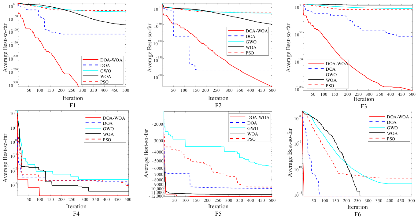
$F_6\left(x\right)=-20\exp \left(-0.2\sqrt{{\displaystyle \frac{1}{n}}{\displaystyle {\sum }_{i=1}^n{x}_i^2}}\right)-\exp \left({\displaystyle \frac{1}{n}}{\displaystyle {\sum }_{i=1}^n\cos \left(2\pi x_i\right)}\right)+20+e$	30	$\left[-32,32\right]$	0

were selected to examine the search accuracy and stability of the DOA-WOA. Functions F1–F4 contain a single optimum and were used to evaluate exploitation performance, whereas F5 and F6 were employed to examine the ability to escape local optima. The DOA-WOA was compared with the DOA [22], WOA [21], GWO [23], and PSO [24] under an identical population size of 30 and a maximum of 500 iterations. Each algorithm was independently executed 30 times, and the resulting mean and standard deviation were used to evaluate solution quality and repeatability.

All algorithms were run in MATLAB 2024b with Intel(R) i7 14650H CPU, 32RAM, and Windows 11 Education.

The numerical results in

Table 3. Comparisons Between the DOA-WOA and Four Other Algorithms Across Six Tests.

F	DOA-WOA		DOA		WOA		GWO		PSO
	AVE	STD	AVE	STD	AVE	STD	AVE	STD	AVE	STD
F1	0.00 × 100	0.00 × 100	1.20 × 10−47	2.69 × 10−47	5.97 × 10−78	1.12 × 10−77	2.27 × 10−27	3.03 × 10−27	5.20 × 10−23	5.17 × 10−23
F2	4.26 × 10−210	0.00 × 100	1.55 × 10−65	3.46 × 10−65	2.61 × 10−52	4.72 × 10−52	1.06 × 10−16	6.02 × 10−17	2.19 × 10−13	2.29 × 10−13
F3	2.50 × 10−153	5.60 × 10−153	7.27 × 10−27	1.63 × 10−26	6.91 × 101	7.56 × 100	7.12 × 10−7	4.86 × 10−7	2.97 × 10−9	2.58 × 10−9
F4	4.76 × 10−5	5.09 × 10−5	4.02 × 10−4	1.16 × 10−4	1.72 × 10−3	1.10 × 10−3	1.80 × 10−3	9.60 × 10−4	1.57 × 10−3	7.92 × 10−4
F5	−1.19 × 104	9.73 × 102	−9.14 × 103	2.54 × 103	−1.09 × 104	1.08 × 103	−6.34 × 103	8.95 × 102	−8.61 × 103	3.51 × 102
F6	4.44 × 10−16	0.00 × 100	4.98 × 10−16	0.00 × 100	5.42 × 10−15	1.94 × 10−15	1.07 × 10−13	2.20 × 10−14	1.90 × 10−12	7.05 × 10−13

show that the DOA-WOA obtains the lowest or near-lowest objective values on the six functions while maintaining relatively small inter-run variations. The convergence trajectories in Figure 6 further indicate that the hybrid update mechanism improves the search process on both unimodal and multimodal functions. The Wilcoxon results provide additional statistical evidence for these differences, although significant superiority is not observed under every comparison condition.

Statistical significance analysis was conducted to evaluate the performance differences between the DOA-WOA and the comparison algorithms. To reduce the influence of random initialization, each algorithm was independently executed 30 times under the same experimental settings. In addition to the mean and standard deviation, the Wilcoxon signed-rank test was employed to assess the statistical significance of the results. The significance level was set to ($\alpha <0.05$), and a (p)-value lower than 0.05 indicates a statistically significant difference.

The Wilcoxon signed-rank test results in

Table 4. Wilcoxon signed-rank test results for DOA-WOA against the comparison algorithms.

Function	DOA	WOA	GWO	PSO
F1	+	+	+	+
F2	+	+	+	+
F3	+	+	+	+
F4	+	+	+	+
F5	+	=	+	+
F6	=	+	+	+
+/=/− 1	5/1/0	5/1/0	6/0/0	6/0/0

¹ “+”, “=”, and “−” indicate that the DOA-WOA performs significantly better than, shows no statistically significant difference from, and performs significantly worse than the corresponding comparison algorithm, respectively, at the significance level of α = 0.05.

further show that the DOA-WOA significantly outperforms the GWO and PSO on all six functions. Significant improvements are also obtained over the DOA and WOA on five of the six functions, while no statistically significant differences were observed between the DOA-WOA and DOA on F6 or between the DOA-WOA and WOA on F5. Therefore, the statistical results generally confirm the optimization advantage of the DOA-WOA, although its superiority is not statistically significant under every test condition.

3.2. Clustering Identification Based on a Gaussian Mixture Model

The low-dimensional customer features obtained by t-SNE are further clustered using a GMM to recover the transformer–customer affiliations. Let $Y={\left\{y_i\right\}}_{i=1}^N$ denote the embedded feature set, where each mixture component represents a customer group associated with one distribution transformer. The probability density of customer feature $y_i$ is expressed as:

$$p\left(x\right)={\displaystyle \sum _{k=1}^K{\pi }_k}\mathcal{N}(Y_i\mid {\mu }_k,{\mathsf{\Sigma }}_k),$$

(12)

where $K$ is the number of Gaussian components; ${\pi }_k$ is the weight of component $k$, satisfying ${\displaystyle {\sum }_{k=1}^K{\pi }_k}=1$; and ${\mu }_k$ and ${\sum }_k$ are its mean vector and covariance matrix, respectively. In this study, $K$ is set equal to the recorded number of distribution transformers. Therefore, the current formulation considers transformer–customer identification under the condition that the cluster number is known and the recorded transformer-count information is available and reliable.

Considering that correlations may still exist between different feature dimensions in the low-dimensional space, and to avoid local optimum issues caused by random initialization, the full covariance matrix form is selected for the model’s covariance matrix, and the K-means++ strategy is introduced to initialize the GMM.

Furthermore, during the expectation–maximization (EM) iteration process, the covariance matrix may become singular or ill-conditioned due to highly concentrated sample distributions or insufficient sample quantities. To address this, a regularization treatment is introduced in the covariance estimation procedure:

$${\Sigma }_k^{reg}={\Sigma }_k+\lambda I,$$

(13)

where ${\Sigma }_k^{reg}$ is the regularized covariance matrix, $I$ is the identity matrix, and $\lambda >0$ is the regularization coefficient.

3.3. Steps of the Proposed Method

A transformer–customer relationship identification method based on high-dimensional data feature embedding and a Gaussian Mixture Model clustering is proposed. The flowchart of the proposed transformer–customer relationship identification method is illustrated in Figure 2. The specific procedural steps are as follows:

Step 1. Sample the raw voltage data of each customer from AMI and construct the original customer feature matrix.

Step 2. Using the silhouette coefficient after K-means clustering as the objective function, the DOA-WOA is employed to adaptively optimize the perplexity and learning rate parameters of t-SNE.

Step 3. Apply the t-SNE algorithm to perform nonlinear dimensionality reduction on the original feature matrix, obtaining the low-dimensional embedding features of the customers.

Step 4. Construct a Gaussian Mixture Model, initialize the model parameters, and perform clustering identification by incorporating the low-dimensional embedding features.

Step 5. Based on the Gaussian Mixture Model clustering results, map the customer cluster labels to the corresponding distribution transformer area numbers, thereby establishing the affiliation relationships between customers and distribution transformers.

It should be noted that the computational procedure of the proposed method includes t-SNE hyperparameter optimization, nonlinear dimensionality reduction, and GMM-based clustering identification. The DOA-WOA-based hyperparameter search constitutes the main computational cost because multiple candidate parameter combinations need to be evaluated. After the optimal t-SNE parameters are determined for a given dataset, the subsequent dimensionality-reduction and clustering process only requires one t-SNE execution and one GMM fitting procedure. Therefore, the computational cost of the complete parameter-optimization and identification process is distinguished from that of a single identification execution in the following complexity and runtime analyses.

3.4. Computational Complexity Analysis

The computational cost of the proposed method mainly consists of DOA-WOA-based t-SNE hyperparameter optimization, t-SNE dimensionality reduction, and GMM clustering. The notations used in the complexity analysis are summarized in

Table 5. Notations used in the computational complexity analysis.

Symbol	Description
$N$	Number of customers
$d$	Dimension of the embedded feature space generated by t-SNE
$P$	Population size of the DOA-WOA
$T$	Maximum number of optimization iterations
$K$	Number of transformer areas (clusters)
$I$	Number of EM iterations in the GMM algorithm

.

The DOA-WOA optimization process represents the most computationally intensive component of the proposed framework. Each population individual requires one evaluation of the t-SNE embedding and the corresponding clustering quality during the optimization procedure. Since the t-SNE computation dominates the evaluation cost, the computational complexity of the optimization process can be approximated as O($P\cdot T\cdot N^2$).

The transformer–customer relationship identification process mainly involves t-SNE dimensionality reduction and GMM clustering after the optimal hyperparameters are obtained. A single execution of t-SNE has a computational complexity of approximately O($N^2$). The GMM algorithm performs clustering in the low-dimensional embedding space with a complexity of O($I\cdot K\cdot N\cdot d^2$). Since $d$ = 2 or 3 in this study, the clustering complexity can be simplified to O($I\cdot K\cdot N$).

The overall computational complexity of the proposed method can therefore be expressed as O($P\cdot T\cdot N^2+I\cdot K\cdot N$). The first term generally dominates the total computational cost because the population-based optimization process repeatedly performs t-SNE embedding and clustering-quality evaluation under different candidate parameter combinations. By contrast, once the hyperparameters have been obtained, the computational cost of a single identification process mainly consists of one t-SNE embedding and the subsequent GMM clustering. The corresponding runtime and the influence of customer scale are further evaluated in Section 5.3.

4. Simulation Verification

A simulated low-voltage distribution transformer area dataset is established for method validation. The identification performance is subsequently assessed under different voltage-data missing rates and measurement-error levels.

4.1. Results of Data Dimensionality Reduction

The simulated LVDS consists of eight transformers and 1371 customers, with voltage measurements collected over 288 time periods. The dataset is embedded into a three-dimensional space using t-SNE, whose hyperparameters are optimized by the WOA and DOA-WOA, respectively. To examine the optimization behavior under random initialization, each optimization algorithm is independently executed 50 times. The run which achieved the best objective value was selected solely to visualize the three-dimensional embedding results. In contrast, the quantitative transformer–customer relationship identification results reported in Section 4.2 are obtained by averaging 10 independent identification runs.

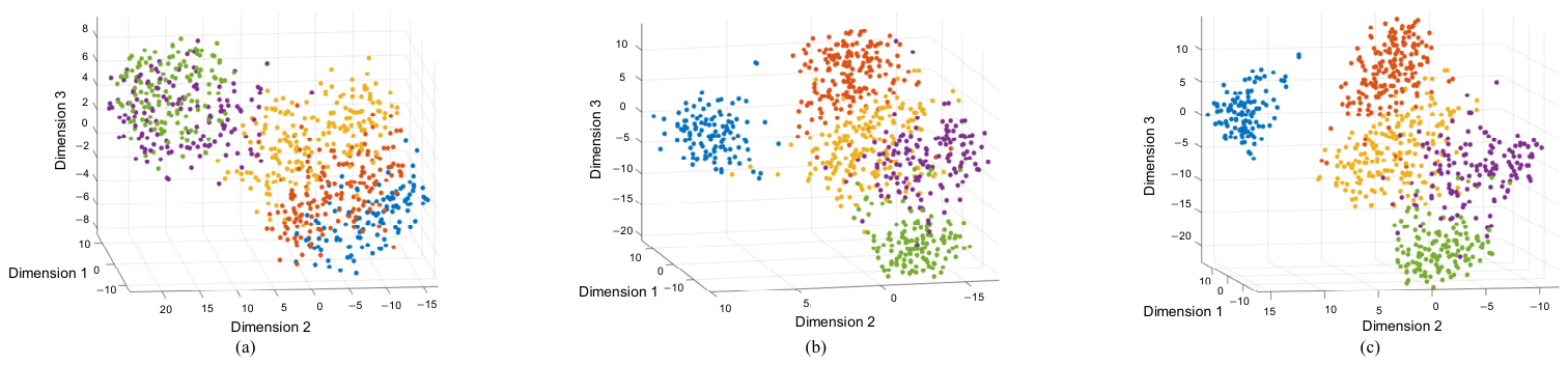
Figure 7 compares the t-SNE embedding results obtained without parameter optimization, with WOA-based optimization, and with DOA-WOA-based optimization. For visual clarity, the figure displays five transformer groups, with a distinct color assigned to each group. Substantial cluster overlap and unclear boundaries are observed in Figure 7a. The separability is improved in Figure 7b, whereas Figure 7c shows the clearest inter-cluster separation and intra-cluster compactness.

4.2. Results of Clustering Identification

The evaluation metrics include label-aligned recognition accuracy, Adjusted Rand Index (ARI), and the Fowlkes–Mallows Index (FMI) [25]. Higher ARI and FMI values indicate greater consistency between the identified and reference groupings. Each method was independently executed 10 times on the same dataset under identical parameter settings, and the mean results are reported in

Table 6. Mean statistical results of clustering methods.

Method	Accuracy	FMI	ARI
t-SNE-GMM	85.6	0.929	0.828
WOA-t-SNE-GMM	98.6	0.978	0.929
DOA-WOA-t-SNE-GMM	99.2	0.991	0.950

.

The experimental results show that, compared with t-SNE-based clustering using default parameters, parameter optimization significantly improves all evaluation metrics, indicating that appropriate parameter selection can effectively enhance the low-dimensional embedding quality. Consequently, the proposed method achieves nearly 100% recognition accuracy under ideal conditions.

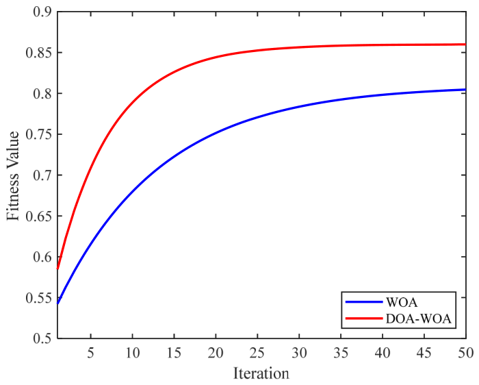
As shown in Figure 8, both algorithms improve the fitness value during iteration. The DOA-WOA increases faster and converges to a higher value than the WOA, with final fitness values of approximately 0.86 and 0.80, respectively. This indicates that the DOA-WOA has better optimization accuracy and can obtain more suitable t-SNE parameters, thereby improving low-dimensional cluster separability and supporting more accurate GMM (Gaussian Mixture Model)-based identification.

To investigate the influence of customer scale on computational cost, customer subsets containing 100, 300, 500, 700, 1000, and 1371 customers were constructed from the simulated dataset. For each subset, the voltage-data length, sampling configuration, population size, maximum optimization iterations, and other algorithm parameters were kept unchanged. Customers were proportionally sampled from different transformer areas to maintain a similar cluster distribution. For each customer scale, the complete optimization–identification procedure was independently executed 10 times under the same hardware and algorithm settings, and the average computational time was reported.

As shown in

Table 7. Computational time under different customer scales.

Number of Customers	Average Optimization Time/s	Average Identification Time/s	Total Computational Time/s
100	69.3	1.17	70.47
300	212.1	3.15	215.25
500	356.7	4.98	361.68
700	502.4	6.75	509.15
1000	722.2	9.30	731.50
1371	995.7	12.36	1008.06

, both the hyperparameter optimization time and the single-dataset identification time exhibit an overall increasing trend with the number of customers. The identification time includes both the t-SNE dimensionality-reduction process and the subsequent Gaussian Mixture Model (GMM) clustering process. When the customer scale increases from 100 to 1371, the total computational time increases from approximately 70.47 s to 1008.06 s. The optimization stage accounts for more than 98% of the total runtime because each candidate parameter combination requires repeated t-SNE embedding and clustering-quality evaluation. Although the measured runtime does not exhibit a strictly quadratic increase within the tested customer range, its increasing trend is consistent with the complexity analysis in Section 3.4. The difference between the theoretical complexity and the measured growth rate is mainly attributable to the limited test scale, algorithm convergence behavior, and fixed computational overhead.

4.3. Sensitivity Analysis

In practical engineering applications, voltage data acquisition may suffer from missing measurements or measurement errors, both of which can affect the identification results. Therefore, multiple statistical models were constructed using simulated data to investigate the influence of different factors on the performance of the proposed identification method.

The transformer–customer relationship identification performance of different methods was evaluated using the simulated LVDS data. The following four identification methods are compared and analyzed:

Method 1: K-means clustering using correlation features extracted from customer voltage profiles [26].

Method 2: Gaussian Mixture Model clustering-based identification after t-SNE dimensionality reduction with default parameters.

Method 3: Gaussian Mixture Model clustering-based identification after t-SNE dimensionality reduction with WOA-optimized parameters.

Method 4: Gaussian Mixture Model clustering-based identification after t-SNE dimensionality reduction with DOA-WOA-optimized parameters, as proposed in this study.

(1)

Sensitivity analysis in case of missing voltage data

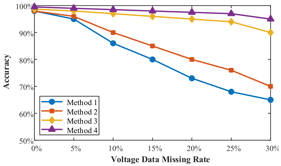
To evaluate the robustness of the proposed method under incomplete voltage measurements, different missing rates ranging from 0% to 30% were introduced into the simulated dataset. As shown in Figure 9, the identification accuracy of Method 4 remains relatively stable as the missing rate increases, whereas the accuracy of the other methods shows a more obvious decline. This result indicates that the proposed method is less sensitive to missing voltage data and maintains better identification performance under data incompleteness.

(2)

Sensitivity to measurement data errors

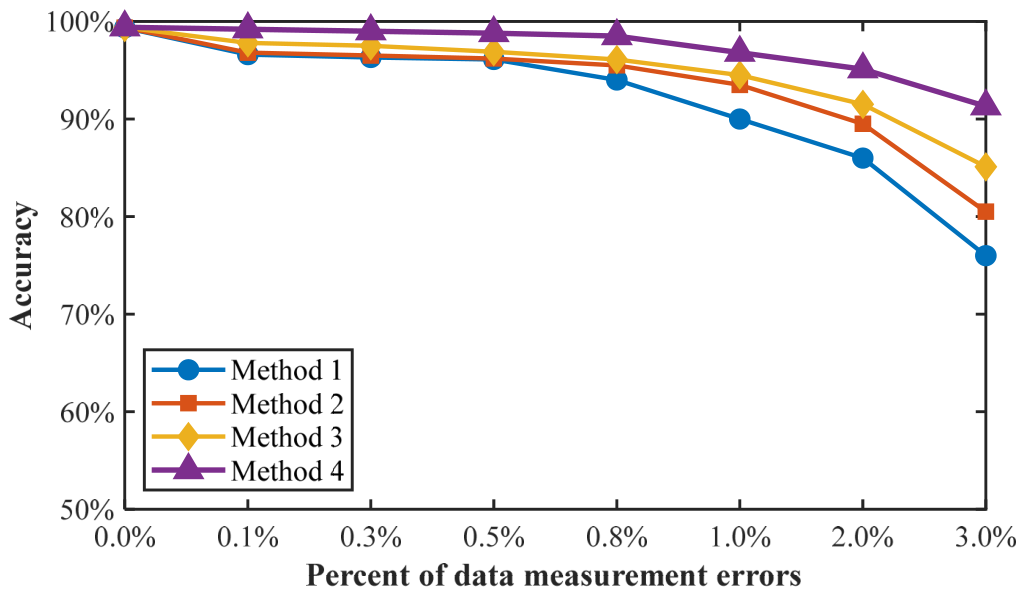
Voltage-measurement uncertainty is examined by introducing error levels ranging from 0% to 3% into the simulated dataset. This range extends beyond the ±0.5% accuracy level specified in ANSI C12.20 [27], allowing the methods to be evaluated under both normal and degraded metering conditions. As shown in Figure 10, the identification accuracy of all four methods decreases with increasing measurement error. Nevertheless, Method 4 retains the highest accuracy and exhibits the smallest performance loss throughout the tested range, including at error levels above 0.5%, indicating lower sensitivity to voltage-measurement errors.

5. Experiment and Result Analysis

5.1. Experimental Case 1

5.1.1. Case Description

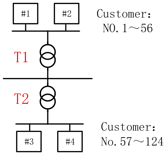
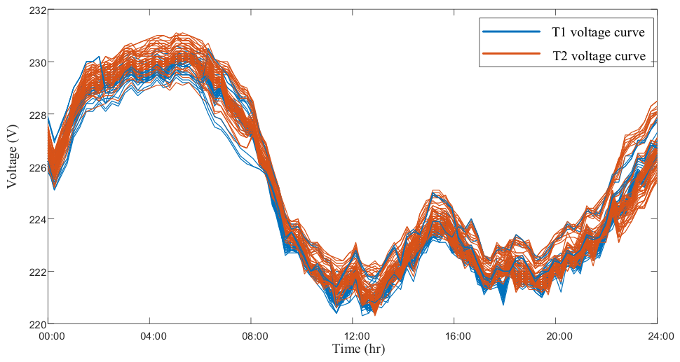
The data for Case Study 1 were obtained from the State Grid Electricity Information Collection System, and comprised time-series voltage data from two low-voltage distribution transformers and 124 low-voltage customers in a residential community in Zhejiang Province in May 2025. The sampling interval for the voltage data is 15 min, resulting in 96 samples per day. The low-voltage topological structure of the transformer areas is shown in Figure 11. The typical 24 h voltage profiles of customers from the two areas are illustrated in Figure 12.

5.1.2. Dimensionality Reduction and Clustering Results

According to the t-SNE algorithm, perplexity affects the balance between local and global structures, while the learning rate influences the stability and convergence of dimensionality reduction. Therefore, the search ranges of perplexity and learning rate were set to [20, 80] and [100, 300], respectively. The optimal parameter combination was obtained using the DOA-WOA and then applied to the dimensionality reduction in the raw voltage data.

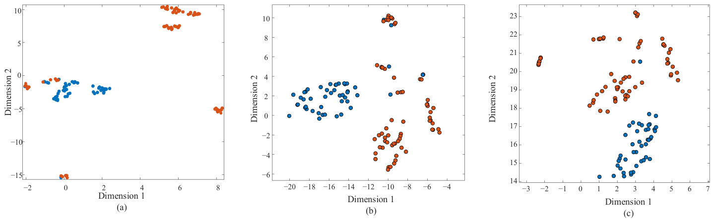
Two-dimensional visualization is shown in Figure 13. From the comparative results, it can be observed that while UMAP presents a relatively clear global structure, it exhibits some outliers and an overlap of samples from different transformer areas. With default t-SNE parameters, the blue samples form a distinct cluster, and the orange samples are distributed across multiple clusters; however, a considerable degree of localized intermixing exists between the two categories of labels. In contrast, the t-SNE mapping optimized by the DOA-WOA yields more compact clusters with virtually no overlap between samples from different transformer areas. Therefore, t-SNE with parameter optimization can enhance the clusterability of the two-dimensional embedding space, providing a more stable and well-separated feature foundation for the subsequent Gaussian Mixture Model-based clustering identification.

Table 8. Evaluation indicators for dimensionality reduction effect.

	Algorithm	UMAP	t-SNE	DOA-WOA-t-SNE
Index
SC		0.8928	0.9129	0.9245
DBI		0.5838	0.4845	0.4669

presents a quantitative analysis of the clustering structure quality after feature embedding using the silhouette coefficient (SC) and the Davies–Bouldin Index (DBI). The SC simultaneously reflects intra-cluster compactness and inter-cluster separation; a larger SC value indicates a clearer cluster structure in the embedding space. Conversely, a smaller DBI value signifies tighter intra-cluster compactness and greater inter-cluster separation. As shown in the table, compared to UMAP and t-SNE with default parameters, the two-dimensional representation space obtained after DOA-WOA parameter optimization exhibits stronger intra-cluster aggregation and inter-cluster separability, which is beneficial for improving the accuracy of clustering identification.

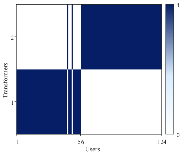
After obtaining two-dimensional representation, a Gaussian Mixture Model is employed to perform clustering identification on the customer samples. A full covariance matrix is adopted for the model, which is initialized using the K-means++ strategy. The number of clusters is set to $K=2$. The model parameters are estimated iteratively via the EM algorithm, and a regularization treatment is applied during covariance estimation with a regularization coefficient of $\lambda ={10}^{-5}$. The cluster label for each customer is obtained. The identification results, representing the affiliation between the identified transformer areas and the customers, are expressed as a 0–1 matrix. Its corresponding heatmap is shown in Figure 14.

Figure 14 presents the heatmap of the identification results for Case Study 1. The results show that only two customers under transformer T1 are misidentified as belonging to transformer area T2, while all other customers are correctly identified. The achieved identification accuracy is 98.4%. For the practical dataset containing 124 customers, the average runtime of the complete optimization–identification procedure was 87.72 s, including 86.30 s for hyperparameter optimization and 1.42 s for single-dataset identification.

5.1.3. Contrast Experiment

Transformer–customer relationship identification mainly involves two key procedures: feature representation construction and customer clustering. To evaluate the effectiveness of the proposed framework, comparative experiments are conducted under the same input data and cluster-number settings. Different combinations of dimensionality reduction, parameter optimization, and clustering strategies are used to assess the contribution of the proposed DOA-WOA-optimized t-SNE and GMM (Gaussian Mixture Model)-based identification framework. The number of clusters is set according to the number of transformers, and the performance is evaluated using FMI, ARI, and accuracy. The comparative results are reported in

Table 9. Identification results of combination methods.

Transformer–Customer Relationship Identification Method	FMI	ARI	Accuracy (%)
PCA + K-means	0.843	0.811	85.7
UMAP + K-means	0.887	0.847	90.9
t-SNE + GMM	0.923	0.882	95.1
WOA-t-SNE + GMM	0.961	0.928	97.1
DOA-WOA-t-SNE + GMM (proposed)	0.976	0.944	98.4

.

As shown in Table 9, the proposed DOA-WOA-t-SNE-GMM method achieves the highest accuracy, FMI, and ARI among the compared methods. Compared with the conventional t-SNE-GMM and WOA-t-SNE-GMM methods, the proposed method provides more accurate and consistent clustering results. A detailed discussion of the performance differences, the respective roles of t-SNE parameter optimization and GMM clustering, and a comparison with existing studies is presented in Section 5.3.

5.2. Experimental Case 2

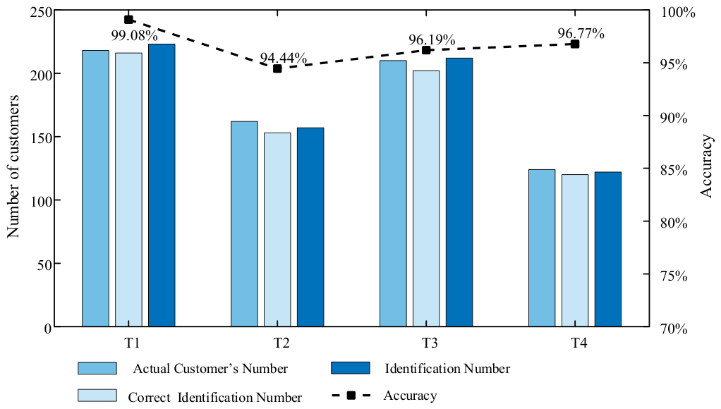
The data for Case Study 2 were obtained from multiple transformer areas in a certain location in Zhejiang Province for December 2025. The two practical cases were collected from geographically distinct locations in Zhejiang Province. The community consists of four LV distribution transformers and 714 LV customers, of which about 220 customers under transformer T3 have 5–30% of data missing. This case aims to verify the effectiveness of the proposed method in large-scale LVDSs under conditions of missing data.

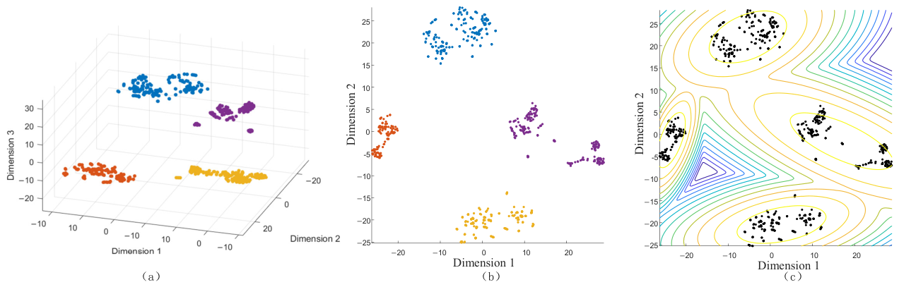
By optimizing the t-SNE of the parameters, the best $\left[p,\eta \right]$ parameter was identified as $\left[45,240\right]$. Figure 15 presents the t-SNE feature embedding visualization under the optimal parameter combination, showing the clustering visualization results of the three-dimensional feature embedding.

The low-dimensional feature matrix is inputted into the Gaussian Mixture Model to obtain the cluster labels. Figure 16 shows a bar chart of the recognition results for multiple areas. In the case of data loss in the LVDS, the proposed method achieved an average accuracy of 96.8%, indicating that the method is still suitable. For the practical dataset containing 714 customers, the average optimization time and single-dataset identification time were 512.60 s and 6.87 s, respectively, resulting in a total runtime of 519.47 s.

The runtime results of the two practical cases are generally consistent with the customer-scale analysis presented in Section 4.2, showing that the computational time increases with the number of customers. The hyperparameter optimization stage accounts for most of the total runtime, whereas the subsequent single-dataset identification process requires considerably less time. Although the proposed method is not intended for strict real-time identification, its computational cost remains acceptable for offline archive verification and periodic transformer–customer relationship updating.

5.3. Discussion and Analysis of Results

The results in Table 8 indicate that the identification performance is jointly affected by the dimensionality-reduction method, parameter configuration, and clustering model. PCA mainly preserves linear variance information, whereas conventional UMAP and t-SNE may provide insufficient separation when fixed parameters are used. By adaptively optimizing the perplexity and learning rate, the proposed method improves the compactness of customers supplied by the same transformer and reduces the overlap between different transformer areas.

The comparison between t-SNE-GMM and DOA-WOA-t-SNE-GMM shows that t-SNE parameter optimization is an important source of performance improvement because the clustering model remains unchanged. GMM further improves customer assignment by describing each transformer area with an individual mean and covariance matrix, making it more suitable for clusters with unequal dispersion or partially overlapping boundaries. Since the dimensionality-reduction and clustering methods are not independently varied in all comparison groups, their separate numerical contributions cannot be fully isolated. Nevertheless, optimized t-SNE and GMM act at different stages and play complementary roles.

Compared with the physical-model-based methods in [10,11,12], the proposed method reduces the dependence on complete network parameters and synchronized branch measurements. Unlike the learning-based methods in [13,14,15], it does not require a large labeled training dataset. Compared with the similarity-based clustering methods in [16,17,18], it first constructs a more separable nonlinear feature space and then performs probabilistic clustering, rather than directly clustering high-dimensional voltage sequences using fixed similarity measures. These comparisons are methodological, and no direct numerical superiority across different datasets is claimed.

The two practical datasets were collected from geographically distinct locations in Zhejiang Province rather than from the same residential community or local distribution area. Case Study 1 contains two distribution transformers and 124 customers, whereas Case Study 2 contains four distribution transformers and 714 customers and further includes missing voltage measurements for part of the customers. The differences in geographical location, system scale, data-collection period, and data completeness provide evidence that the proposed method is not restricted to a single community, transformer area, or specific dataset. Together with the simulation results under different customer scales, missing-data rates, and measurement-error levels, these practical cases demonstrate the robustness and cross-site applicability of the method under the tested conditions. Nevertheless, both datasets were collected within Zhejiang Province. Therefore, the current results do not yet constitute comprehensive evidence of cross-provincial or cross-utility generalizability, which should be further evaluated using distribution systems with different network structures, customer compositions, voltage characteristics, and measurement conditions.

6. Conclusions

This study developed a data-driven method for transformer–customer relationship identification using AMI voltage measurements. The proposed framework employs t-SNE to obtain low-dimensional representations of customer voltage profiles, adaptively optimizes the perplexity and learning rate using the DOA-WOA, and subsequently applies a GMM to identify customer groups associated with different distribution transformers.

The simulation results show that the proposed method achieved an identification accuracy of 99.2%, together with a Fowlkes–Mallows Index of 0.991 and an Adjusted Rand Index of 0.950. It also maintained relatively stable identification performance under the tested voltage-data missing rates of up to 30% and measurement-error levels of up to 3%. In the two practical cases, identification accuracies of 98.4% and 96.8% were obtained, respectively. Comparisons with the default-parameter t-SNE method and the Whale Optimization Algorithm-based method demonstrate that adaptive hyperparameter optimization improves the compactness and separability of the low-dimensional voltage features, thereby providing a more distinguishable feature space for subsequent Gaussian Mixture Model clustering. The two practical cases required 86.3–512.6 s for hyperparameter optimization but only 1.42–6.87 s for a single identification process after the optimal parameters had been determined. Therefore, the current method is more suitable for offline archive verification and periodic transformer–customer relationship updating than for strict real-time identification.

Several limitations remain and will be addressed in future work. Although the two practical datasets were collected from geographically distinct locations in Zhejiang Province and differed in transformer number, customer scale, data-collection period, and data completeness, broader generalizability across provinces, utilities, and network environments requires further validation. Moreover, the current method assumes that the number of distribution transformers is known, while t-SNE hyperparameter optimization accounts for most of the computational cost. Future studies will therefore validate the method on distribution systems with different structures and customer scales, investigate automatic cluster-number determination based on the Bayesian information criterion (BIC) and Akaike information criterion (AIC), and compare the DOA-WOA with grid search and modern hyperparameter optimization methods. Dynamic topology tracking, multi-source measurement integration, and deep representation learning will also be explored to improve computational efficiency and adaptability.

References

1. Mokhtar, M.; Robu, V.; Flynn, D.; Higgins, C.; Whyte, J.; Loughran, C.; Fulton, F. Automating the Verification of the Low Voltage Network Cables and Topologies. IEEE Trans. Smart Grid 2019, 11, 1657–1666. [Google Scholar] [CrossRef]
2. Li, Z.; Tan, M.; Jiang, W.; Lv, X.; Liu, W.; Chen, J. A Review of Topology Identification Methods and Applications for Low Voltage Distribution Networks. Energy Rep. 2026, 15, 108914. [Google Scholar] [CrossRef]
3. Häberle, V.; Tayyebi, A.; He, X.; Prieto-Araujo, E.; Dörfler, F. Grid-Forming and Spatially Distributed Control Design of Dynamic Virtual Power Plants. IEEE Trans. Smart Grid 2023, 15, 1761–1777. [Google Scholar] [CrossRef]
4. Zhang, H.; Zhao, J.; Wang, X.; Xuan, Y. Low-Voltage Distribution Grid Topology Identification with Latent Tree Model. IEEE Trans. Smart Grid 2022, 13, 2158–2169. [Google Scholar] [CrossRef]
5. Erseghe, T.; Tomasin, S.; Vigato, A. Topology Estimation for Smart Micro Grids via Powerline Communications. IEEE Trans. Signal Process. 2013, 61, 3368–3377. [Google Scholar] [CrossRef]
6. Pappu, S.J.; Bhatt, N.; Pasumarthy, R.; Rajeswaran, A. Identifying Topology of Low Voltage Distribution Networks Based on Smart Meter Data. IEEE Trans. Smart Grid 2017, 9, 5113–5122. [Google Scholar] [CrossRef]
7. Balakrishna, P.; Rajagopal, K.; Swarup, K. Distribution Automation Analysis Based on Extended Load Data from AMI Systems Integration. Int. J. Electr. Power Energy Syst. 2017, 86, 154–162. [Google Scholar] [CrossRef]
8. Liao, W.; Yang, D.; Wang, Y.; Ren, X. Fault Diagnosis of Power Transformers Using Graph Convolutional Network. CSEE J. Power Energy Syst. 2020, 7, 241–249. [Google Scholar] [CrossRef]
9. Cavraro, G.; Bernstein, A.; Kekatos, V.; Zhang, Y. Real-Time Identifiability of Power Distribution Network Topologies with Limited Monitoring. IEEE Control Syst. Lett. 2019, 4, 325–330. [Google Scholar] [CrossRef]
10. Zhao, J.; Xu, M.; Wang, X.; Zhu, J.; Xuan, Y.; Sun, Z. Data-Driven Based Low-Voltage Distribution System Transformer-Customer Relationship Identification. IEEE Trans. Power Deliv. 2021, 37, 2966–2977. [Google Scholar]
11. Hu, H.; Zhao, J.; Bian, X.; Xuan, Y. Transformer-Customer Relationship Identification for Low-Voltage Distribution Networks Based on Joint Optimization of Voltage Silhouette Coefficient and Power Loss Coefficient. Electr. Power Syst. Res. 2023, 216, 109070. [Google Scholar] [CrossRef]
12. Liu, L.; Shi, N.; Wang, D.; Ma, Z.; Wang, Z.; Reno, M.J.; Azzolini, J.A. Voltage Calculations in Secondary Distribution Networks via Physics-Inspired Neural Network Using Smart Meter Data. IEEE Trans. Smart Grid 2024, 15, 5205–5218. [Google Scholar] [CrossRef]
13. Ni, Q.; Jiang, H. Topology Identification of Low-Voltage Distribution Network Based on Deep Convolutional Time-Series Clustering. Energies 2023, 16, 4274. [Google Scholar] [CrossRef]
14. Huang, L.; Zhou, G.; Zeng, Y.; Zhang, J.; Feng, Y. Transformer-Customer Relationship Identification Based on Deep Gaussian Mixture Model in Low-Voltage Distribution System. Electr. Power Syst. Res. 2024, 234, 110591. [Google Scholar] [CrossRef]
15. Tang, H.; Xu, T.; He, Z.; Li, Y.; Cui, L. Topology Identification of Low-Voltage Distribution Network Nodes and Dynamic Adjustment of User Nodes Based on LSTM-GCN. Electr. Power Syst. Res. 2026, 253, 112566. [Google Scholar] [CrossRef]
16. Al Khafaf, N.; Song, H.; McGrath, B.; Jalili, M. Identification of Low Voltage Distribution Transformer–Customer Connectivity Based on Unsupervised Learning. Energy Rep. 2023, 9, 72–79. [Google Scholar] [CrossRef]
17. Lei, Y.; Yang, F.; Feng, Y.; Hu, W.; Cheng, Y. Two-Stage Transformer–Customer Relationship Identification Strategy for Low-Voltage Distribution Grid Using Physics-Guided Graph Attention Network. Energies 2025, 18, 4380. [Google Scholar] [CrossRef]
18. Li, J.; Yao, X.; Liu, B. Identification of Low-Voltage Distribution Substation Topology Based on User Profile. Front. Energy Res. 2024, 12, 1427986. [Google Scholar] [CrossRef]
19. Van der Maaten, L.; Hinton, G. Visualizing Data Using T-SNE. J. Mach. Learn. Res. 2008, 9, 2579–2605. [Google Scholar]
20. Kobak, D.; Berens, P. The Art of Using T-SNE for Single-Cell Transcriptomics. Nat. Commun. 2019, 10, 5416. [Google Scholar] [CrossRef] [PubMed]
21. Mirjalili, S.; Lewis, A. The Whale Optimization Algorithm. Adv. Eng. Softw. 2016, 95, 51–67. [Google Scholar] [CrossRef]
22. Lang, Y.; Gao, Y. Dream Optimization Algorithm (DOA): A Novel Metaheuristic Optimization Algorithm Inspired by Human Dreams and Its Applications to Real-World Engineering Problems. Comput. Methods Appl. Mech. Eng. 2025, 436, 117718. [Google Scholar] [CrossRef]
23. Mirjalili, S.; Mirjalili, S.M.; Lewis, A. Grey Wolf Optimizer. Adv. Eng. Softw. 2014, 69, 46–61. [Google Scholar] [CrossRef]
24. Jiao, J.; Ghoreishi, S.; Moradi, Z.; Oslub, K. Coupled Particle Swarm Optimization Method with Genetic Algorithm for the Static–Dynamic Performance of the Magneto-Electro-Elastic Nanosystem. Eng. Comput. 2022, 38, 2499–2513. [Google Scholar]
25. Fowlkes, E.B.; Mallows, C.L. A Method for Comparing Two Hierarchical Clusterings. J. Am. Stat. Assoc. 1983, 78, 553–569. [Google Scholar] [CrossRef]
26. Ahmed, M.; Seraj, R.; Islam, S.M.S. The K-Means Algorithm: A Comprehensive Survey and Performance Evaluation. Electronics 2020, 9, 1295. [Google Scholar] [CrossRef]
27. Etezadi-Amoli, M.; Ghofrani, M.; Arabali, A. Performance of Advanced Meters: Effects of Different Temperatures and Loading Conditions on Meter Accuracy. In Proceedings of the 2014 IEEE PES T&D Conference and Exposition; IEEE: New York, NY, USA, 2014; pp. 1–5. [Google Scholar]
Figure 1. Topology of low-voltage distribution system.
Energies 19 03427 g001
Figure 2. Flowchart of the proposed transformer–customer relationship identification method. The colored voltage curves represent different customers, while the colored points and symbols represent different sample groups or clusters during the dimensionality reduction and clustering processes. The colors are used only for visual distinction and do not indicate specific physical meanings.
Energies 19 03427 g002
Figure 3. Flowchart of the dimensionality reduction process using a parameter-optimized t-SNE. Solid arrows indicate the data processing flow, whereas the dashed arrow represents the optimization of the t-SNE hyperparameters by the DOA-WOA algorithm.
Energies 19 03427 g003
Figure 4. Flowchart of the DOA-WOA. “Y” denotes “Yes” and indicates the execution of the Yes branch; “N” denotes “No” and indicates the execution of the No branch.
Energies 19 03427 g004
Figure 5. Flowchart of t-SNE parameter optimization based on DOA-WOA. The rounded rectangles represent the start and end of the flowchart, the rectangles represent the processing operations, and the dashed rectangle indicates the iterative optimization process of the fitness function evaluation.
Energies 19 03427 g005
Figure 6. Convergence curves of five algorithms for six representative test functions.
Energies 19 03427 g006
Figure 7. Visualization results of dimensionality reduction for five selected transformers: (a) t-SNE; (b) WOA-t-SNE; (c) DOA-WOA-t-SNE. The different colored dots represent customer samples belonging to different distribution transformer clusters. Each color corresponds to a specific cluster identified by the clustering algorithm.
Energies 19 03427 g007
Figure 8. WOA and DOA-WOA convergence curve for t-SNE parameter optimization.
Energies 19 03427 g008
Figure 9. Identification accuracy of four methods with different voltage data missing rates.
Energies 19 03427 g009
Figure 10. Performance comparison of different methods under different measurement-error levels.
Energies 19 03427 g010
Figure 11. Topology model of low-voltage distribution system.
Energies 19 03427 g011
Figure 12. Time-series voltage curve of low-voltage distribution customers.
Energies 19 03427 g012
Figure 13. Two-dimensional visualization of embedded features obtained by different methods: (a) UMAP; (b) t-SNE; (c) DOA-WOA-t-SNE. Different colors represent users belonging to different transformer areas.
Energies 19 03427 g013
Figure 14. Heatmap of the identification results for Case Study 1.
Energies 19 03427 g014
Figure 15. Visualization results (a) 3D scatter plot of user clusters; different colored dots represent users belonging to different transformer regions (Cluster 1 to 4); (b) 2D projection of the user clusters; (c) Gaussian probability density contour lines (colored curves) overlaid with the user clusters.
Energies 19 03427 g015
Figure 16. The identification results for Case Study 2.
Energies 19 03427 g016