A Novel Vibration Centroid-Based Approach for Fault Diagnosis of Transformer Winding

Abstract

Tank vibrations of a power transformer, originating primarily from winding vibration and core vibration through mechanical coupling and fluid–structure interaction, are regarded as essential carrier signals for assessing the integrity of the winding. To improve the diagnostic accuracy of winding condition, this paper presents a vibration centroid-based diagnostic model that integrates feature fusion from vibration signals. According to the frequency spectrum of vibration signals obtained using Zoom-FFT, a set of new spatial vibration feature vectors—namely vibration centroid coordinates and Boyce-Clark shape index—were defined. This approach converts spatially distributed vibration signals into compact and discriminate indicators. A diagnostic model was subsequently constructed by integrating the grey wolf optimization (GWO) algorithm with the least squares support vector machine (LSSVM), ensuring that optimal classification performance was achieved. No-load, short-circuit, and load tests were made on a 35 kV-rated oil-immersed transformer. During the experiments, the transformer winding was divided into four categories: healthy condition, winding looseness, axial deformation, and radial deformation. The proposed GWO-LSSVM-based classifier was trained and tested using the defined vibration feature vectors. The results indicate that the proposed method achieves superior performance, with a recognition rate of 98.44%, and offers high efficiency.

1. Introduction

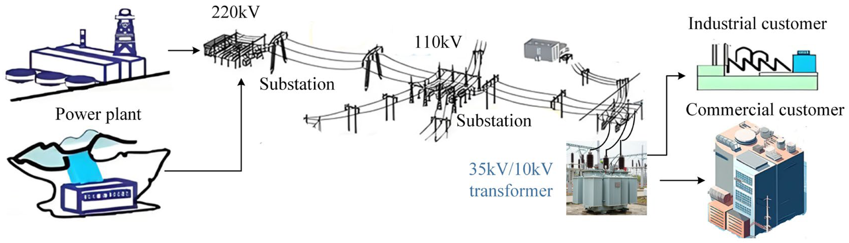
As an indispensable component of the new-generation power grid, the power transformer plays a critical and non-substitutable role in voltage transformation and energy regulation. During operation, the power transformer is continuously subjected to the interrelated electrical, thermal, magnetic, and mechanical stresses, leading to the inevitable aging of insulation and then the occurrence of transformer failures. Among them, winding deformation caused by external short-circuit impacts is consistently reported as the most prevalent category, accounting for approximately 30% [1,2]. Meanwhile, it is important to recognize that slight winding looseness or deformation is an inevitable occurrence in the operation of aging transformers. The transition towards “double-high” power systems fundamentally alters the electrical and mechanical environment for power transformers. Beyond traditional short-circuit threats, transformer windings also endure broad-spectrum harmonic forces, high di/dt transient impacts, and cumulative fatigue from frequent power-electronic-switching-induced transients [3]. This presents new challenges for mechanical integrity assessment and deformation prevention. Specifically, the 35 kV-rated oil-immersed three-phase transformer constitutes a critical asset in medium-voltage power distribution networks. Serving as a critical link between high-voltage transmission systems (110/220 kV) and low-voltage distribution feeders (10/0.4 kV), as illustrated in Figure 1, these transformers are deployed across diverse operational scenarios, including urban distribution substations, industrial zones, manufacturing complexes, and renewable energy collection systems like wind farm clusters and photovoltaic plant step-up stations. Unlike transmission-level units, distribution-level 35 kV transformers generally lack comprehensive real-time monitoring systems, making them more susceptible to winding deformation when subjected to harmonic-rich load currents and frequent short-circuit impulses. Hence, timely and accurate assessment of transformer winding condition is imperative, particularly in modern power grids where electrical stresses are increasingly severe.

The traditional diagnostic methods for winding deformation are mainly composed of short-circuit impedance (SCI) [4,5,6], frequency response analysis (FRA) [7,8,9,10], and sweep frequency impedance (SFI) analysis [11,12]. These diagnostic techniques primarily detect the variations in electrical parameters of transformer winding, like the inductance, capacitance, and resistance, through distinct principles. Specifically, a quantifiable metric with clear pass/fail thresholds for the SCI method has been defined by international standards (e.g., IEC 60076-5) [4], making it excellent for identifying gross deformations. In contrast, the FRA method constructs a high-resolution “electromagnetic fingerprint” of transformer winding, typically 1 Hz to 2 MHz, exhibiting exceptional sensitivity to a wide range of mechanical faults, including axial displacement and radial buckling. A central challenge lies in the interpretive process, which relies heavily on expert-driven comparison with a baseline. By integrating the two approaches, SFI analysis measures the winding impedance across the range from low to medium-high frequencies (e.g., 50 Hz to several kHz). With the advantage of higher sensitivity than SCI and better noise immunity than FRA, SFI analysis is particularly effective at detecting incipient winding failures. Nevertheless, its application is constrained by reduced sensitivity to capacitance-altering faults and by the current absence of a unified framework for the quantitative morphological analysis of its impedance spectrum.

Vibrations in an operating transformer originate mainly from the windings and the core. These vibrations transmit through insulation oil and solid structural components of the transformer, ultimately manifesting as measurable vibrations on the transformer tank. Owing to its non-intrusive nature, practicality, and ease of deployment, the vibration analysis technique has become a predominant approach in monitoring the winding condition. Given the inherently nonlinear and non-stationary nature of vibration signals, existing studies have predominantly focused on two interconnected aspects: discriminative feature extraction [13,14,15,16,17,18,19,20,21,22,23,24] and the reliable formulation of a diagnostic model [25,26,27,28,29,30,31]. This paper reviews recent typical studies in this field. As illustrated in

Table 1. Studies on identifying the winding conditions of a transformer using vibration signals.

Refs	Features and Diagnosis	Validation	Tested Transformer	Contribution and Evaluation
[13,14]	Method: FFT Parameter: average displacement	Laboratory experiment	Transformer model with both healthy and deformed windings	A correlation was found between winding deformation and a pronounced rise in vibration displacement using an optical-based Fiber Bragg Grating sensor.
[16]	Method: FFT Parameter: Vibration main fundamental Ratio and vibration entropy	Short-circuit impulse experiment	A D-400/6.3 transformer model: 400 kVA, 0.4 kV/6.3 kV	The progressive deformation of transformer winding was identifiable, with weak feature transferability.
[19]	Method: FFT Parameter: harmonic-to-fundamental ratio from three sensors Classifier: XGBoost	Laboratory experiment	An SFZ10-31500/110 three-phase oil-immersed transformer	The classification accuracy exceeded 99% in identifying winding looseness, with weak transferability across different load currents.
[20]	Method: FFT Parameter: triangle normal vector at 50i Hz	Laboratory and field experiments	Two three-phase transformers: 500 kVA, 15 kV/400 V and 50 MVA, 110 kV/10 kV	The accuracy for identifying the abnormal conditions of transformer winding exceeded 100%, with several accelerometers.
[21]	Method: EWT and multiscale entropy Parameter: multiscale entropy of all selected EWF components	Simulation signal	-	The accuracy for identifying the abnormal conditions of transformer winding exceeded 100%.
[23]	Method: ISGMD-PCA Parameter: dimension-reduced eigenvector initially constructed by parameters in the time domain Classifier: ELM	Laboratory experiment	A single-phase transformer model: 10 kV	The amplitude drift parameter increased by 5% under slight deformation. The accuracy for short-circuit withstand ability exceeds 98%.
[24]	Method: FFT and WVD-FCM Parameter: membership degree matrix obtained by FCM algorithm	Short-circuit impulse experiment	A SFSZ7-31500/110 transformer	Both the high-frequency component (>400 Hz) of the vibration signal and membership degree revealed cumulative winding deformation.
[25,26]	Method: RMS and FFT Parameter: frequency response function, vibration image Classifier: GRU, CNN	Laboratory and field experiments	Laboratory: A single-phase transformer model: 10 kV, 415/240 V Field: A three-phase transformer: 110 kV	The CNN-based classifier achieved an accuracy rate of over 98% in identifying abnormal conditions of transformer winding.
[27]	Parameter: time domain Classifier: GRU	Laboratory experiment	A three-phase transformer model: 0.4 kV	The classifier achieved a relative absolute error of 0.56% in predicting excitation voltage.
[28]	Parameter: time domain Classifier: a deep noisy filtering diagnostic model	Laboratory experiment	A three-phase transformer model: 10 kV/0.4 kV	The classifier achieves both the highest valuation index and the best stability.
[29]	Method: GAF encoding method Classifier: an improved atrous deep residual network	Laboratory experiment	Three-phase transformer: 10 kV/400 V	The classifier achieved an accuracy rate of over 98% in identifying the failures of winding and core.
[30]	Parameter: time domain Classifier: ConvNeXt	Laboratory experiment	Three-phase transformer: 10 kV/400 V	The accuracy for identifying the winding looseness exceeded 97%.
[31]	Parameter: time domain Classifier: memory-enhanced DSN	Laboratory experiment	Three-phase transformer: 10 kV/400 V	The classifier achieved an accuracy rate of over 99% in identifying the failures of winding and core.

, frequency-domain features obtained through Fast Fourier Transform (FFT) have drawn primary interest to derive indicators for recognizing abnormal winding conditions. Nevertheless, constrained by the time-frequency uncertainty principle, the product of the time-domain and frequency-domain window widths is always no less than 1/2, indicating that high temporal and high frequency resolutions cannot be achieved concurrently. As a result, the traditional FFT always yields an average spectrum. To better capture the time-varying features in transformer vibration signals, time-frequency analysis methods, such as empirical wavelet transform (EWT), improved symplectic geometry mode decomposition (ISGMD) algorithm, and Wigner-Ville Distribution (WVD), were applied to decompose the vibration signals in the time-frequency domain. In addition, vibration signals were also converted into two-dimensional images, offering a superior visual representation for capturing the variations in vibration signals across both time and frequency domains.

Meanwhile, high diagnostic accuracy for winding faults has been achieved by both machine learning (ML) classifiers (e.g., XGBoost and extreme learning machine (ELM)) and deep learning (DL)-based classifiers (e.g., gated recurrent unit (GRU), convolutional neural network (CNN), ConvNeXt, and memory-enhanced dual-stream network (DSN)). Generally, DL-based techniques exhibit stronger automatic feature learning and representation capabilities directly from raw or minimally processed data, effectively forming an end-to-end learning paradigm from data to decision. However, this capacity comes at the cost of heavy computational burdens, dependency on large-scale datasets, and limited model interpretability. These challenges become particularly pressing given that the winding faults of an operating transformer are, after all, low-probability events. In contrast, ML-based approaches rely critically on well-defined and discriminative features extracted from raw data. This reliance results in models that are inherently more interpretable, more computationally efficient, and require reduced data requirements for training, demonstrating higher compatibility with resource-limited deployment in transformer winding diagnosis.

In summary, current methodologies for identifying the winding faults of transformers are constrained by the following limitations: (1) vibration signals collected from the transformer tank belong to ex situ measurements. Much of the existing literature always relies on the vibration signal from a single accelerometer adhered to the transformer tank. This approach sometimes introduces uncertainty to a certain degree and then degrades the diagnostic accuracy. The authors have observed a similar scenario during a short-circuit impact test on a 220 kV-rated transformer, where the limitations of single-point monitoring were conclusively demonstrated. (2) Extracting the well-defined and discriminative features from vibration signals that account for spatial properties is crucial. (3) Developing a diagnostic model for winding faults that ensures high recognition accuracy with the constraints of resource-limited deployment presents a significant challenge.

To address these limitations, this study proposes the following key improvements and contributions to the fault diagnosis of transformer winding:

(1)

A diagnostic model was developed by integrating the grey wolf optimization (GWO) algorithm with least squares SVM (LSSVM), driven by the proposed vibration feature vectors. This model demonstrated superior accuracy and generalization, making it particularly valuable for practical field deployment feasibility of a vibration-based monitoring system.

(2)

Vibration feature vectors, including the coordinates of the vibration centroid and the Boyce-Clark shape index, were proposed based on a multi-point accelerometer layout and the amplitude of the fundamental frequency of vibration signals, providing a new spatial dimension for feature parameters of vibration signals.

(3)

Enhanced frequency resolution and amplitude accuracy were achieved by applying the Zoom-FFT technique to the vibration signals, providing computational efficiency for practical field deployment. The resulting detailed spectral information is critical for accurate transformer winding diagnosis.

(4)

A comprehensive comparison was conducted, demonstrating the superior performance of the proposed spatial vibration feature vectors combined with the GWO-LSSVM-based classifier over conventional methods for diagnosing the transformer winding.

This paper is structured as follows. Section 2 describes the vibration features of the transformer both theoretically and experimentally. Section 3 establishes the methodology, including feature extraction of vibration signals and construction of the GWO-LSSVM-based classifier. Section 4 presents the results of the proposed method. Section 5 provides a discussion. Finally, the conclusions of this work are presented in Section 6.

2. Vibration Features of Transformer

2.1. Theoretical Analysis of Transformer Vibration

Transformer vibrations originate primarily from the core and windings. Core vibration stems from magnetostriction of the silicon steel and electromagnetic forces generated by the alternating magnetic flux between and within the core laminations. Among these factors, magnetostriction of the silicon steel is the dominant factor in core vibration, and the deformation of the silicon steel satisfies,

$${\displaystyle \frac{1}{L}}{\displaystyle \frac{dL}{dH}}={\displaystyle \frac{2{\epsilon }_s}{H_c^2}}\left|H\right|$$

(1)

where $L$ and ${\epsilon }_s$ are the original axial dimension and saturation magnetostriction of the silicon steel sheet, respectively, $H$ is the magnetic field intensity, and $H_c$ is the coercive force.

Based on the magnetostriction principle, the magnetostriction coefficient quantitatively describes the induced mechanical strain per unit of magnetic field strength. It exhibits inherent nonlinearity, which is determined by both the mechanical stress and the magnetic field strength, expressed as follows.

$$\lambda ={\displaystyle \frac{\Delta L}{L}}={\displaystyle \frac{2{\epsilon }_s}{H_c^2}}{\displaystyle {\int }_0^H\left|H\right|}dH={\displaystyle \frac{{\epsilon }_s}{H_c^2}}{H}^2$$

(2)

where $\lambda$ is the magnetostriction coefficient, and $\Delta L$ is the dimensional change in the silicon steel.

The operation of a power transformer is fundamentally based on Faraday’s law of electromagnetic induction. Given the excited voltage of a power transformer as $U=U_0\sin \omega t$, where $U$ and $U_0$ are the amplitude and RMS of the excited voltage, respectively, $\omega$ is the angular frequency, the magnetostriction coefficient in Equation (2) can be rewritten as

$$\lambda ={\displaystyle \frac{\Delta L}{L}}={\displaystyle \frac{{\epsilon }_s}{H_c^2}}{({\displaystyle \frac{B}{\mu }})}^2={\displaystyle \frac{{\epsilon }_s}{{(\mu H_c)}^2}}{\displaystyle \frac{U_0^2}{{(N_{1}S\omega )}^2}}{\sin }^2\omega t$$

(3)

where $B$ is the magnetic flux intensity, $\mu$ is the magnetic permeability, $N_1$ is the number of turns in the coil, and $S$ is the cross-sectional area penetrated by the magnetic flux.

Given the $B-H$ hysteresis loop of silicon steel under alternating magnetization, the magnetic permeability is inherently time-dependent. Accordingly, the vibration acceleration of the transformer core is given by

$$a_c={\displaystyle \frac{d^2\Delta L}{d{t}^2}}={\displaystyle \frac{L{\epsilon }_s{U}_0^2}{{(N_{1}S{H}_c)}^2}}\left({\displaystyle \frac{2\cos 2\omega t}{{\mu }^2}}-{\displaystyle \frac{4\sin 2\omega t}{\omega {\mu }^3}}{\displaystyle \frac{d\mu }{dt}}+{\displaystyle \frac{(\cos 2\omega t-1)}{{\omega }^2{\mu }^3}}{\displaystyle \frac{d^2\mu }{d{t}^2}}-{\displaystyle \frac{3-3\cos 2\omega t}{{\mu }^4}}{\left({\displaystyle \frac{d\mu }{dt}}\right)}^2\right)$$

(4)

where $a_c$ is the vibration acceleration of the transformer core.

When neglecting the hysteresis effect, it can be seen that the vibration acceleration of the core is predominantly composed of spectral components at the fundamental frequency of 100 Hz (for a 50 Hz power system) or 120 Hz (for a 60 Hz power system) and its integer harmonics. However, due to factors such as hysteresis effect, electromagnetic forces, clamping condition, and overall structure of the iron core, vibration acceleration of the transformer core, measured from the no-load test of the transformer, typically exhibits more dominant features at the integer harmonics like 300 Hz, 400 Hz, and 500 Hz. This phenomenon is particularly noticeable in aged transformers.

Transformer windings are commonly configured with the high-voltage winding in a continuous disk-type arrangement and the low-voltage winding in a helical type, respectively. When the load current flows through the transformer winding and interacts with the surrounding leakage magnetic field, dynamic electromagnetic (Lorentz) forces are generated. These forces act between distinct windings, across individual winding disks, and upon adjacent conductor turns, thereby inducing the winding vibration. Since the electromagnetic force on the coil is proportional to the current squared, the vibration acceleration of the transformer winding can be described by

$$a_w\propto F_w\propto I_m^2\cos [1+\cos (2\omega t)]$$

(5)

where $a_w$ is the vibration acceleration of the transformer winding, $F_w$ is the electromagnetic force, and $I_m$ is the RMS value of the load current.

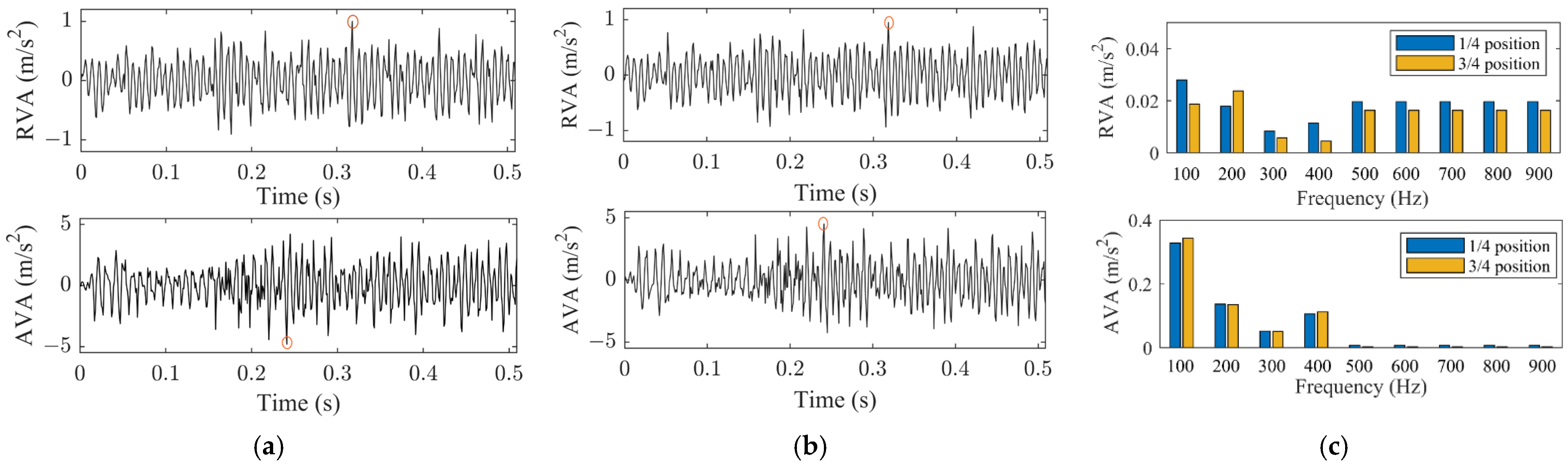
For clarity, taking the high-voltage winding of an oil-immersed transformer as an example, its vibration acceleration at different positions of the transformer winding was calculated through the finite element analysis method, and the results, including time-domain waveforms at typical positions and the corresponding frequency spectra, are illustrated in Figure 2 [32]. In the figure, AVA and RVA denote axial and radial vibration acceleration of the transformer winding, respectively. The peaks of vibration acceleration are marked with red circles. The 1/4 position and 3/4 position represent the locations at 1/4 and 3/4 of the winding height, respectively, measured from the top of the winding. At these positions, the axial electrodynamic force of the transformer winding reaches its maximum. As can be seen from the figure, the axial vibration intensity of the transformer winding is considerably higher than its radial vibration intensity. The vibration acceleration at the 3/4 position is slightly greater than that at the 1/4 position, caused by the effect of winding gravity. The peaks of vibration acceleration at the 3/4 position corresponding to RVA and AVA are 0.954 m/s2 and 4.513 m/s2, respectively. The frequency spectra of both radial and axial vibration signals are dominated by a 100 Hz component and its higher harmonic components with relatively small proportions. This indicates that the fundamental vibration response of the transformer winding is primarily at twice the power frequency (100 Hz), consistent with theoretical analysis and previously reported results. When collecting the vibration signals on the transformer tank, it is recommended to place the vibration accelerometers around these positions to achieve optimal fault diagnosis.

In summary, vibration acceleration of the transformer winding is primarily concentrated at the fundamental frequency of 100 Hz (for a 50 Hz power system) or 120 Hz (for a 60 Hz system) along with a small proportion of integer harmonic frequencies, which can be measured through the short-circuit test. Moreover, the peak-to-peak value, RMS value, and fundamental frequency amplitude of vibration signals caused by winding vibration are each proportional to variations in load current. When a transformer winding loosens or deforms after suffering from the short-circuit, it can be observed that both the overall vibration intensity and the amplitudes at 100 Hz and its integer harmonics, like 200 Hz and 300 Hz, show a significant increase. This phenomenon is primarily attributed to several interconnected factors, such as the structural nonlinearity introduced by displacement and friction caused by loosening of these blocks and the resulting variations in the dynamic features of transformer winding. The latter includes shifts in natural frequencies and variations in vibration modes, governed by the degradation of the winding’s equivalent stiffness and damping properties.

For an operating transformer, vibration signals acquired from the tank surface originate from the nonlinear superposition of core vibration and winding vibration, simultaneously further modulated by the propagation path through internal structural components and insulating oil, the mechanical structure of the transformer tank, and the fluctuated load current. Given that the transformer voltage remains relatively stable under normal operating conditions, the core-induced vibration component can be regarded as a quasi-stationary background within this composite signal. Then, the fault diagnosis of transformer winding can be achieved by tracking the load-dependent vibration feature. In this paper, a methodology to enhance the recognition accuracy for winding condition is presented by comprehensively analyzing spatial features beyond a single-point accelerometer.

2.2. Experimental Analysis of Transformer Vibration

2.2.1. Experimental Description

An experimental object is a real 35 kV-rated oil-immersed transformer with type SZ11-20000/35, whose main parameters are listed in

Table 2. Main parameters of the experimental transformer and reactor.

	Rated Capacity	Rated Voltage (kV)	Rated Current (A)	Reactance (Ω)
Experimental Transformer	20 MVA	35/10.5	329.9/1099.7	11
Reactor	10 Mvar	10.5	549.9	11.02

. The experimental set consisted of a controllable power supply, a step-up transformer, an experimental transformer, adjustable loads, and a measurement system, as illustrated in Figure 1. The on-load, short-circuit, and load tests were conducted by connecting the power supply to the experimental transformer through this intermediate step-up stage. During the load test, two types of loads were connected to the low-voltage side of the experimental transformer. One was a standalone 10.5 kV-rated reactor, labeled as load test 1. The other was a 10.5 kV-rated reactor in parallel with a hollow coil, featuring a resistance of 0.15 Ω at its central tap, labeled as load test 2.

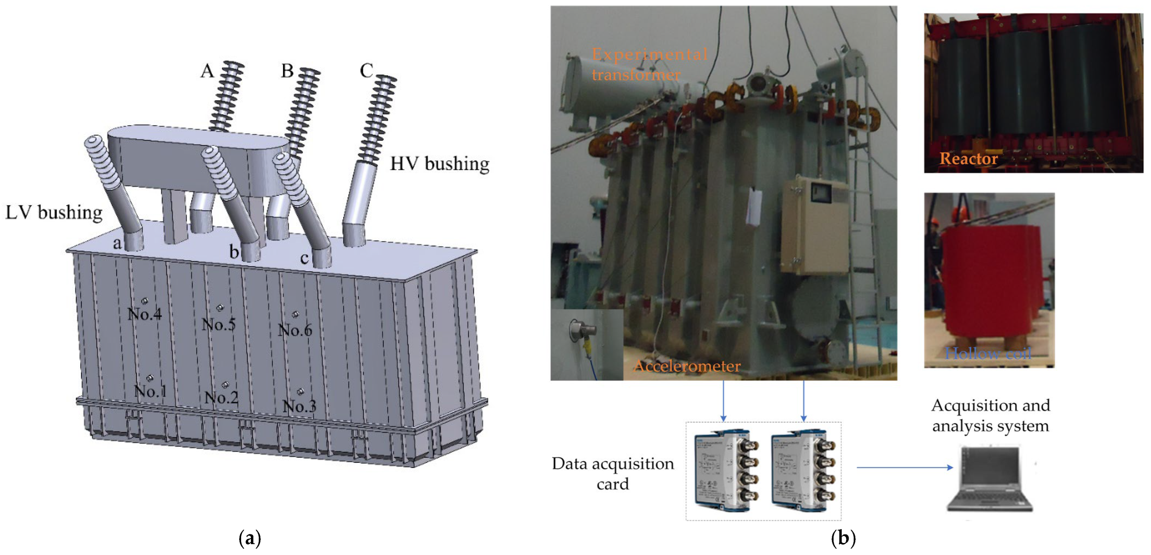
Tank vibrations of a test transformer were measured by six single-axis piezoelectric accelerometers, numbered from No.1 to No.6 and adhered to the transformer tank through the magnetic mount. All accelerometers were PCB 352C33 with a sensitivity of 100 mV/g, a measurement range of ±50 g, and a frequency range from 0.5 Hz to 10 kHz. A photograph of the accelerometer is shown in Figure 3a, where A, B, C and a, b, c denote the high-voltage and low-voltage windings of phase A, B and C, respectively. These accelerometers were vertically installed on the low-voltage side of the transformer tank through the strong magnetic bases to ensure firm contact. Specifically, accelerometers No.1 to No.3 were placed at a distance of 1/4 of the tank height from the bottom, corresponding to phase A, phase B, and phase C, respectively. Accelerometers No.4 to No.6 were placed at a distance of 1/4 of the tank height from the top, also corresponding to phase A, phase B, and phase C, respectively. Here, the locations of accelerometers on the transformer tank are determined according to the mechanical structure of the transformer, simulation of winding vibration, and our prior experience for the measurement of vibration signals from several transformers. That is to say, all selected positions are located at areas of high vibration intensity of the windings while avoiding the reinforcing ribs of the transformer tank.

Additionally, all accelerometers were connected to the NI 9234 modules for vibration signal acquisition and analysis, as illustrated in Figure 3b. The NI 9234 module provides a 24-bit resolution with a maximum sampling rate of 51.2 kS/s per channel, making it suitable for high-precision vibration measurement. The acquisition and analysis system was performed on a computer featuring an Intel Core i5-11400F CPU @ 2.6 GHz, 16 GB of RAM ( Lenovo Group Limited, Beijing, China), and the 64-bit Windows 10 operating system, which was programmed using LabVIEW 2020 (National Instruments, Austin, TX, USA). The sampling frequency of vibration signals was 10 kHz with a duration of 20 s for each group. During the experiments, voltage and current measurements were also performed on the experimental transformer.

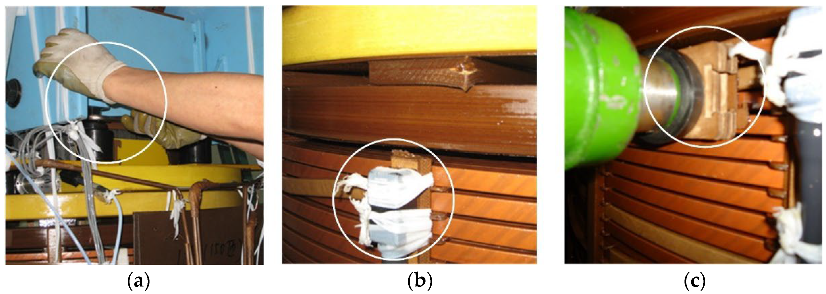
Except for the healthy winding of the experimental transformer (i.e., no winding deformation), three kinds of winding faults were set in the phase C winding of the experimental transformer, namely winding looseness (WL), axial deformation (AD), and radial deformation (RD). Figure 4 shows the real pictures of the preset winding faults on the experimental transformer. Specifically, winding looseness was simulated by reducing the clamping force of the transformer winding to 80% of its designed value. This was achieved by adjusting the clamping bolt between the clamping plate and the winding end ring. Two insulated blocks near the top of phase C winding were removed to simulate the axial deformation. In addition, a small area near the top of phase C winding was jacked inward about 10 cm to simulate the radial deformation. It should be noted that the whole process is time-consuming and costly since the transformer windings are located inside the transformer tank filled with insulated oil. That is to say, prior to performing a fault simulation on the windings, the transformer oil is drained, and the active part is lifted out. Subsequently, the active part is lowered back into the tank, and the insulation oil is refilled.

2.2.2. Experimental Results

In this part, the vibration characteristics of the experimental transformer were investigated under no-load, short-circuit, and load conditions. It is important to note that, for all results presented in this section, the no-load test was conducted at the rated voltage, while the short-circuit test was conducted at the rated current.

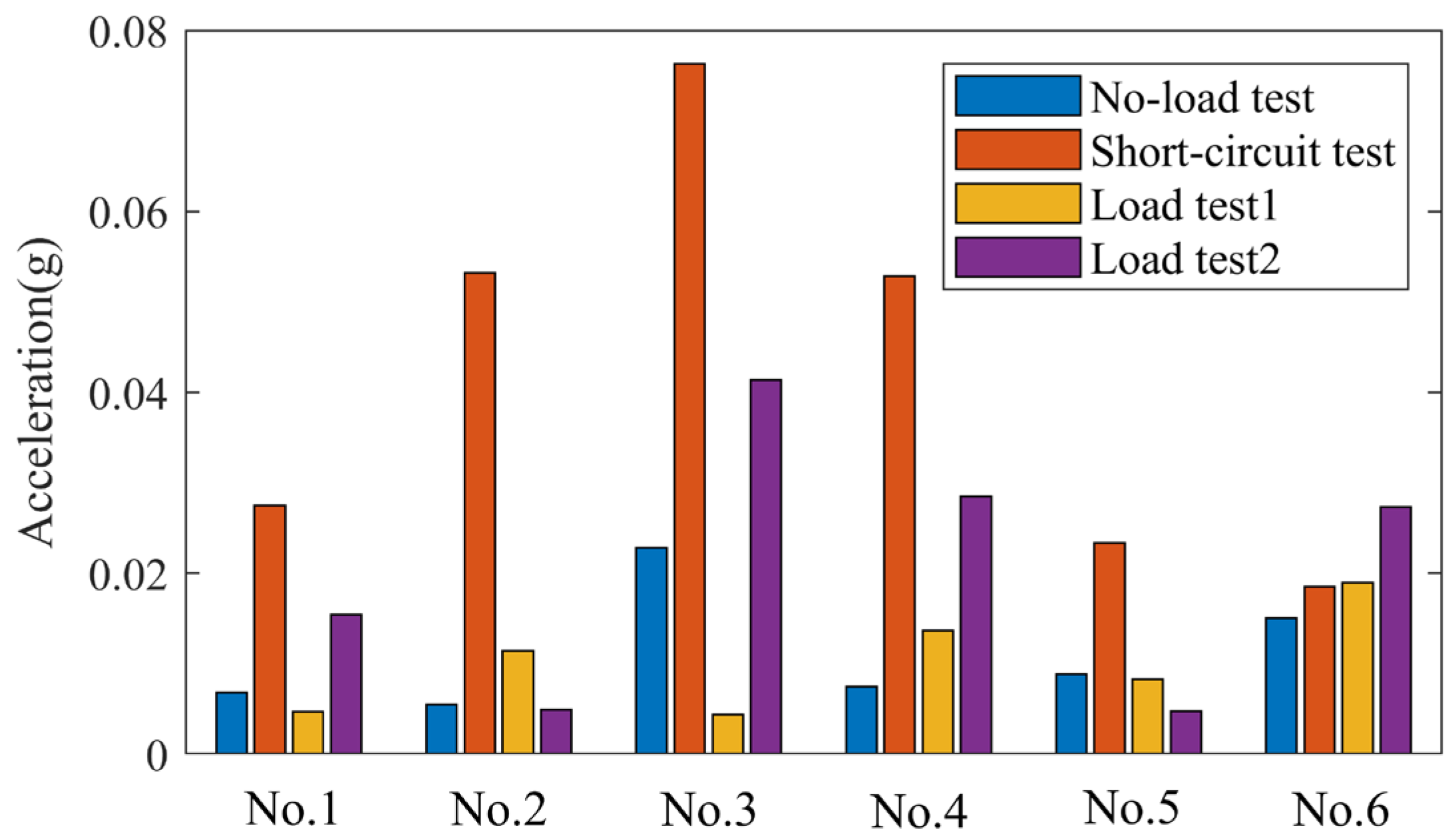
Figure 5 illustrates the vibration amplitude at the fundamental frequency, measured across all accelerometers under the no-load, short-circuit, and load tests for a healthy winding. In the figure, As can be observed from the figure, the amplitudes of the fundamental frequency of vibration signals at all accelerometers are different. Specifically, the amplitudes of the fundamental frequency under the short-circuit test are significantly higher, with the exception of the accelerometer No.6. At this time, tank vibration was primarily contributed by winding vibration. During the load test, the amplitude of the fundamental frequency of vibration signals decreases to varying degrees at accelerometers No.1 to No.5, relative to the short-circuit test. In contrast, during the load test2, the amplitudes of the fundamental frequency at accelerometers No.1, No.2, No.5, and No.6 exceed those recorded in the load test1, a trend attributed to the higher load current.

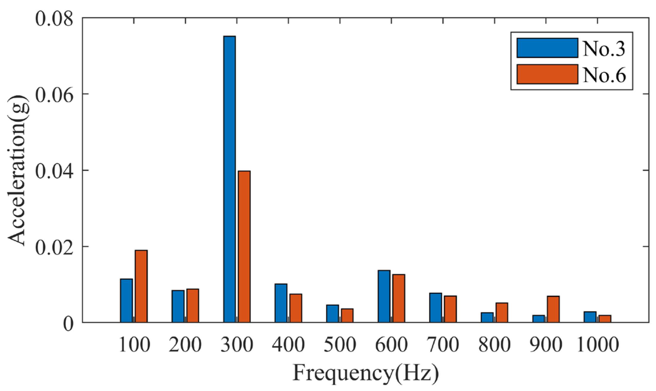
Figure 6 exhibits the frequency spectra of vibration signals measured at accelerometers No.3 and No.6 during the load test1 for a healthy winding. Basically, the difference primarily stems from the vibration response at different locations of the transformer tank. As can be seen from the figure, the frequency spectra of vibration signals are predominantly concentrated on the 100 Hz component and its harmonics, and the amplitudes are maximum at the 300 Hz component. Moreover, the amplitudes of the frequency spectrum at the two accelerometers exhibit significant differences at the 100 Hz and 300 Hz components, indicating variations in vibration response at different locations on the transformer tank when subjected to identical excitation from winding and core vibrations.

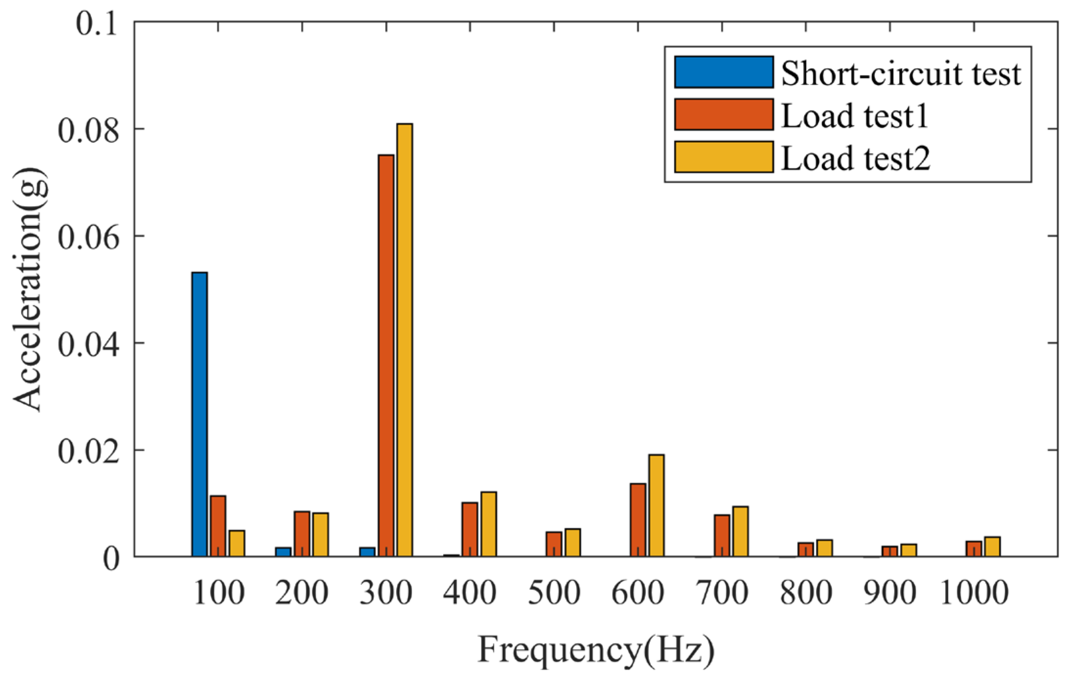
Figure 7 exhibits the frequency spectra of vibration signals measured at accelerometer No.3 during the short-circuit test, load test1 and load test2 for a healthy winding. Here, the differences between the vibration signals result from the different winding currents. As can be seen from the figure, during the short-circuit test, the frequency spectra of the vibration signals are mainly concentrated on the 100 Hz component. During the load test, the frequency spectra of the vibration signals become more complex, with a significant amplitude appearing at the 300 Hz component. When the load current changes, more apparent variations in the amplitude at the 100 Hz component are observed.

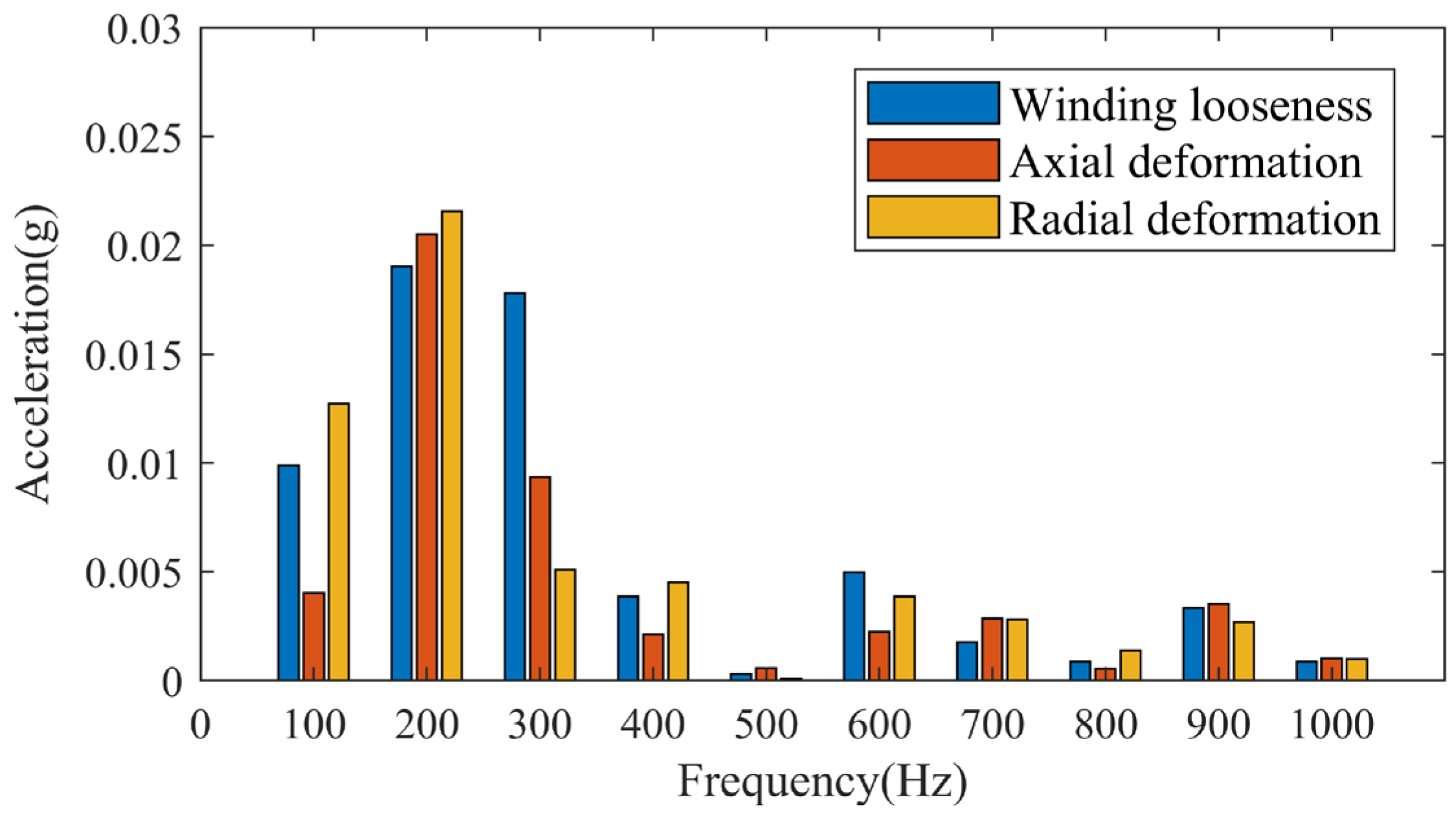
Figure 8 shows the frequency spectra of vibration signals measured at accelerometer No.3 during load test1 under different winding faults. As can be seen from the figure, when the winding conditions change, the frequency spectra of vibration signals exhibit relatively significant variations at 100 Hz, 300 Hz, and 400 Hz components. Compared with the frequency spectrum of the vibration signal at accelerometer No.3 for a healthy winding, the amplitude at the fundamental frequency (i.e., the 100 Hz component) exhibits varying degrees of increase under fault conditions. Especially under winding loosening and radial deformation, the increase in the amplitude of the 100 Hz component is significant.

Based on the combined evidence from the experimental results above and the earlier theoretical analysis, this paper selects the amplitude of the fundamental frequency of vibration signals as a critical feature for subsequent analysis.

3. Methodology

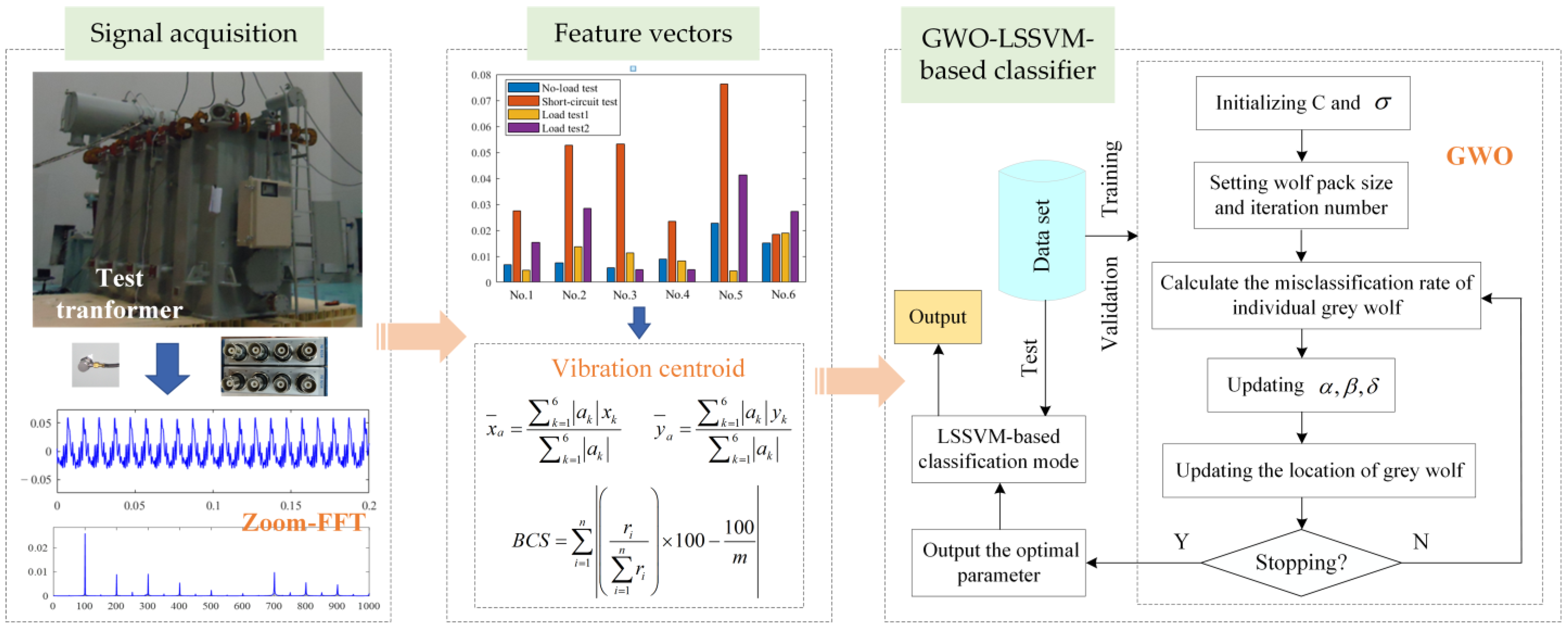
This paper presents a novel approach for fault diagnosis of transformer winding based on the proposed feature vectors and a GWO-optimized LSSVM, and the whole flow chart is illustrated in Figure 9. Specifically, the acquired vibration signals were first processed using the Zoom-FFT technique to obtain the frequency spectrum, where the inherent conflict between the high-resolution spectrum analysis and the practical constraints of limited data length and computational resources was well addressed. The distribution of the vibration centroid and the BCS index were then calculated to characterize the spatial vibration features on the transformer tank, serving as a comprehensive and discriminative indicator of the overall vibration responses with high accuracy. Finally, a GWO-LSSVM-based diagnostic model was developed to identify the winding faults under limited data.

3.1. Zoom-FFT Technique

As a fundamental tool for spectral analysis, the FFT has been widely applied to obtain the frequency spectra of vibration signals of transformers. However, its frequency resolution is inherently constrained by the fundamental relationship Δf = fs/N, where fs denotes the sampling frequency, and N represents the number of data points. It is difficult to achieve finer resolution by simply increasing N due to memory constraints, extended acquisition times, and significantly increased computational burden. Meanwhile, vibration signals of transformers inherently exhibit time-varying features influenced by the fluctuating load currents. Consequently, techniques that enable localized spectral refinement without proportional increases in data length or processing overhead are of importance to carefully analyze the frequency spectra of vibration signals for the fault diagnosis of transformer winding.

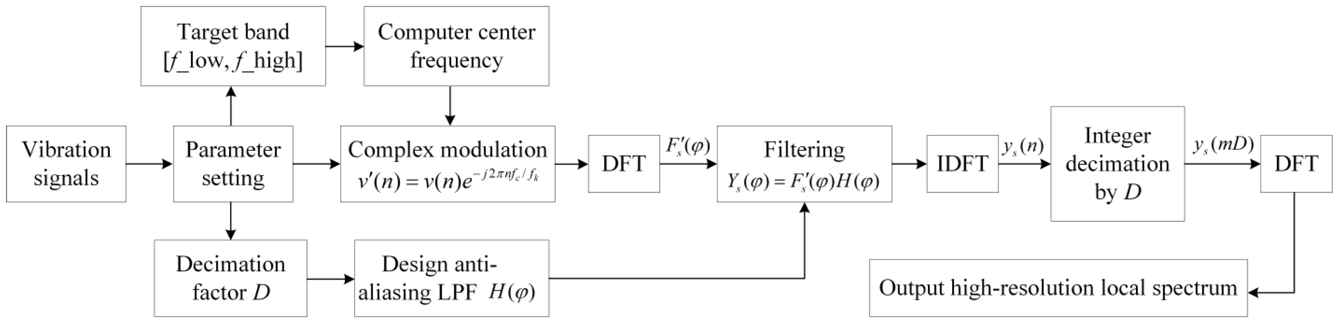
Zoom-FFT technique, also known as the band-selective or frequency-decimation method, was proposed to obtain a high-resolution spectrum through a targeted, multi-step signal processing operation focused on a specific frequency band of interest [f_low, f_high]. Let $v(n),n=1,2,\cdots ,N$ be the vibration signals of the transformer with the sample frequency of fs; the steps of performing spectral analysis using the Zoom-FFT technique are illustrated in Figure 10. In the figure, D denotes the decimation factor, $H(\phi )$ represents the transfer function of the low-pass filter (LPF), DFT and IDFT represent the discrete Fourier transform and inverse discrete Fourier transform, respectively, which can be expressed by

$${F^{\prime }}_s(\phi )={\displaystyle \sum _{n=0}^{N-1}{v^{\prime }}_s(n)e^{-j\frac{2\pi }{N}\phi n}}$$

(6)

$$y_s(n)={\displaystyle \frac{1}{N}}{\displaystyle \sum _{\phi =0}^{N-1}{Y}_s(\phi )e^{j\frac{2\pi }{N}\phi n}}$$

(7)

Using the Zoom-FFT technique, the high-resolution frequency spectra of vibration signals of a transformer can be obtained. Additionally, while a standard FFT requires processing all N samples with $O(N{\log }_{2}N)$ complexity, Zoom-FFT reduces to approximately N/D samples after decimation. This reduction not only decreases computational load but also lowers the memory and data transmission requirements, making it highly suitable for vibration monitoring of transformer winding.

3.2. Vibration Centroid

Tank vibrations of the transformer are mainly excited by the electromagnetic forces from the winding and magnetostriction forces from the core, respectively. Indeed, it is impractical, both physically and economically, to mount accelerometers at every conceivable location on a transformer tank for field deployment. Consequently, a strategically placed finite number of vibration sensors is invariably employed to acquire vibration signals. To overcome the inherent limitation of this sparse spatial sampling and to fully utilize the measured information, a vibration centroid distribution was defined to comprehensively and effectively synthesize a spatial-temporal descriptor. Specifically, a planar coordinate system was established on the transformer tank. Given No.1 as the coordinate origin (0, 0). The line connection from No.1 to No.4 was defined as the positive direction of the y-axis. The line connection from No.1 to No.2 was defined as the positive direction of the x-axis. Then the coordinates of all measured accelerometers within this defined system are listed in

Table 3. Coordinates of all measured accelerometers within the defined system.

Number of Accelerometers	No.1	No.2	No.3	No.4	No.5	No.6
Coordinate	(0, 0)	(2, 0)	(4, 0)	(0, 3)	(2, 3)	(4, 3)

, and the coordinates of the vibration centroid are calculated by the following relations,

$${\overline{x}}_a={\displaystyle \frac{{\displaystyle {\sum }_{k=1}^6\left|a_k\right|x_k}}{{\displaystyle {\sum }_{k=1}^6\left|a_k\right|}}}$$

(8)

$${\overline{y}}_a={\displaystyle \frac{{\displaystyle {\sum }_{k=1}^6\left|a_k\right|y_k}}{{\displaystyle {\sum }_{k=1}^6\left|a_k\right|}}}$$

(9)

where ${\overline{x}}_a$ and ${\overline{y}}_a$ represent the coordinates of the vibration centroid, denoting its specific value on the horizontal axis and vertical axis, respectively; $x_k$ and $y_k$ represent the horizontal coordinate and vertical coordinate of the k-th accelerometer; and $a_k$ refers to the amplitude of the fundamental frequency component of the vibration signals. As discussed in the previous section, the vibration signature of transformer winding is predominantly concentrated at the fundamental frequency. When abnormal conditions, such as winding looseness or deformation, occur, the vibration responses, particularly the amplitude at the fundamental frequency that ultimately reaches the transformer tank, inevitably alter, directly leading to a corresponding shift in the vibration centroid.

In addition, the Boyce-Clark shape (BCS) index was employed to more precisely characterize the variations in vibration centroid distribution. As a landscape ecology metric designed to quantify shape complexity, this index operates by calculating a series of radial distances from the shape’s centroid to its boundary at predefined azimuthal intervals, described by

$$BCS={\displaystyle \sum _{i=1}^n\left|\left(\frac{r_i}{{\displaystyle \sum _{i=1}^n{r}_i}}\right)\times 100-\frac{100}{m}\right|}$$

(10)

where BCS refers to the Boyce-Clark shape index, $r_i$ represents the distance between the shape’s centroid and its boundary, and m is the radial radius.

Generally, a high value of the BCS index indicates a more complex or less compact shape, while a value approaching 1 suggests a highly compact, near-circular form. For this study, the measurement region constituted by the six accelerometers, which were strategically mounted at fixed, pre-selected locations on the transformer tank, is invariable. Under stable electrodynamic and magnetostrictive forces, vibration signals of the transformer exhibit a certain consistent spatial pattern across different accelerometers. However, when winding looseness or deformation occurs, the vibration propagation path is altered, leading to a measurable redistribution of vibration energy. In this context, the BCS index effectively captures such subtle spatial pattern shifts, which are sometimes missed by pointwise spectral features. Meanwhile, the BCS index is inherently invariant to scaling and rotation of the compared shapes. This property is particularly advantageous when comparing vibration signals acquired under varying load currents or from sensors placed at slightly different positions over time, as it focuses purely on the shape of the vibration distribution rather than absolute magnitudes or orientations.

Apparently, the BCS index is able to serve as a reliable and quantifiable indicator for discriminating the winding condition. It is critical to note that the load current of an operating transformer is inherently time-varying, characterized by the continual fluctuations driven by consumer demand and grid conditions. Although the fundamental frequency component of winding vibration is proportional to the square of load current, it is convenient to decouple its influence. For example, the load current of a transformer always exhibits statistical regularity and predictable trends over well-defined time scales. Diurnal and weekly patterns, driven by human activity cycles, are superimposed on longer-term seasonal variations. This structured variability allows for the establishment of a statistical distribution of vibration centroid under normal operational conditions of a transformer. Crucially, the characteristics of this distribution are theoretically distinct from those induced by winding deformation. While load fluctuations in a transformer typically cause variations in the vibration centroid distribution and then the BCS index, such variations are confined to a predictable region correlated with load current. In contrast, winding deformation is prone to induce systematic or sustained displacement of both the vibration centroid distribution and the BCS index. Without timely detection, this shift may continuously deviate from the normal range, thereby decoupling it from the load current.

3.3. A GWO-LSSVM-Based Classifier

3.3.1. LSSVM

LSSVM, a strategically refined variant of the conventional SVM, was selected for classification based on a careful consideration of efficiency, computational complexity, and engineering applicability. Let the training sample be $\left\{\left(x_i,y_i\right)\left|x_i\in R^d,y_i\in R\right.\right\},i=1,2,\cdots ,N_t$, where $x_i$ and $y_i$ represent the input vector and output vector, respectively; d represents the dimension of the sample space, and N_t represents the number of samples. The optimization problem for the LSSVM algorithm is formulated as

$$\min J\left(\omega ,b,{\xi }_i\right)={\displaystyle \frac{1}{2}}{‖\omega ‖}^2+{\displaystyle \frac{C}{2}}{\displaystyle \sum _{i=1}^{N_t}{\xi }_i^2}\hspace{1em}Subject\hspace{0.33em}to\hspace{0.33em}{y}_i\left[\omega \cdot \phi \left(x_i\right)+b\right]=1-{\xi }_i,\hspace{1em}i=1,\cdots ,N_t$$

(11)

where $\omega$ is the weight vector, b is the bias term, C is the penalty factor, ${\xi }_i$ is an error variable, $\phi (\cdot )$ represent the kernel mapping function, and $y_i$ are the class labels.

To solve the constrained problem in Equation (11), Lagrange multipliers ${\alpha }_i$ were always introduced for each equality constraint. Then the Lagrange function can be constructed by adding the constraints, multiplied by their respective ${\alpha }_i$, to the primary objective function, rewritten as

$$L\left(\omega ,b,{\xi }_i,\alpha \right)={\displaystyle \frac{1}{2}}{‖\omega ‖}^2+{\displaystyle \frac{1}{2}}C{\displaystyle {\displaystyle \sum _{i=1}^{N_t}}{\xi }_i^2}-{\displaystyle {\displaystyle \sum _{i=1}^{N_t}}{\alpha }_i\left[y_i\left(\omega \cdot \phi \left(x_i\right)+b\right)-1+{\xi }_i\right]}$$

(12)

where $\alpha ={[{\alpha }_1,{\alpha }_2,\cdots ,{\alpha }_N]}^T$ is the vector of Lagrange multipliers.

The solution is found at the saddle point of the Lagrange function, where the partial derivatives with respect to the primal variables ($\omega ,b,{\xi }_i$) and the variable ${\alpha }_i$ vanish. Setting these derivatives to zero yields the following relations:

$$\left\{\begin{array}{l}{\displaystyle \frac{\partial L}{\partial \omega }}=0\Rightarrow \omega ={\displaystyle \sum _{i=1}^{N_t}{a}_i{y}_i\phi \left(x_i\right)}\\ {\displaystyle \frac{\partial L}{\partial b}}=0\Rightarrow {\displaystyle \sum _{i=1}^{N_t}{a}_i{y}_i=0}\\ {\displaystyle \frac{\partial L}{\partial {\xi }_i}}=0\Rightarrow {\xi }_i=C^{-1}{a}_i\\ {\displaystyle \frac{\partial L}{\partial a_i}}=0\Rightarrow y_i\left[\omega \cdot \phi \left(x_i\right)+b\right]-1+{\xi }_i=0\end{array}\right.$$

(13)

Solving the above equations simultaneously, the decision function for the LSSVM algorithm can be obtained, expressed as

$$f\left(x\right)={\displaystyle \sum _{i=1}^{N_t}{\alpha }_{i}K\left(x_i,x_j\right)+b}$$

(14)

$$K\left(x_i,x_j\right)=\exp \left(-{\displaystyle \frac{{‖x_i-x_j‖}^2}{{\sigma }^2}}\right)$$

(15)

where $K\left(x_i,x_j\right)$ represents the kernel function, employing the radial basis function due to its minimal operational parameters and simple structure, and $\sigma$ is the bandwidth of the kernel function.

Apparently, two critical hyperparameters, namely penalty factor and bandwidth of the kernel function, always determine the performance of the LSSVM-based classifier. Specifically, penalty factor governs the generalization capability of the classifier by regulating the trade-off between minimizing training error and model complexity, and an inappropriate value can lead to overfitting or underfitting. The width of the kernel function directly influences the data distribution in the implicitly mapped high-dimensional feature space, thereby affecting both training stability and predictive behavior. The specific values of these two parameters critically determine the ultimate prediction accuracy of the LSSVM-based diagnostic model. In this paper, the GWO algorithm was employed to perform a global search for the optimal combination of penalty factor and bandwidth of the kernel function.

3.3.2. GWO Algorithm

The GWO algorithm was a swarm intelligence metaheuristic algorithm, inspired by the social hierarchy and cooperative hunting behavior of grey wolf packs in nature. According to the hunting strategies of these packs, this computational framework abstracts the pack’s strict social dominance into a four-tiered mathematical model comprising $\alpha$, $\beta$, $\delta$, and $\omega$ categories, which directly correspond to the fitness ranking of candidate solutions. Within this simulated hierarchy, the $\alpha$ individual, representing the most optimal solution discovered thus far, functions as the primary decision-maker guiding the collective search direction. The $\beta$ and $\delta$ individuals correspond to the second- and third-best solutions, respectively, forming a subordinate leadership circle, while the $\omega$ class encompasses the remaining population members. The core predatory behavior is emulated by defining a dynamic distance metric between the position of each simulated wolf (a potential solution) and the estimated location of the “prey,” which symbolizes the current global optimum within the problem space. The hunting process, which corresponds to the optimization search, is modeled in three main phases:

(1)

Encircling prey

Wolves update their positions to surround the estimated location of the prey. This behavior is modeled by the following relations:

$$\left\{\begin{array}{l}\mathit{D}=\left|\mathit{B}{X}_p\left(t\right)-X\left(t\right)\right|\\ X\left(t+1\right)=X_p\left(t\right)-\mathit{A}\cdot \mathit{D}\\ \mathit{A}=2a{\mathit{r}}_1-a\\ \mathit{B}=2{\mathit{r}}_2\end{array}\right.$$

(16)

where $\mathit{D}$ represents the distance between a grey wolf and its prey, $X(t)$ and $X_p(t)$ denote the positions of a grey wolf and the prey at the t-th iteration, respectively, $X\left(t+1\right)$ represents the new candidate solution position for the next iteration, t is the number of iterations, $\mathit{A}$ is the coefficient vector determining whether the search area expands or contracts, a is a control parameter that decreases linearly from 2 to 0 over the course of iterations, governing the transition from exploration to exploitation, ${\mathit{r}}_1$ and ${\mathit{r}}_2$ are random vectors in [0, 1].

(2)

Hunting (Directed search)

In the GWO algorithm, $\alpha$, $\beta$, and $\delta$ wolves are presumed to possess the best knowledge about the potential location of the prey (optimum). Therefore, the remaining omega wolves update their positions based on the positions of these three leaders:

$$\left\{\begin{array}{l}{D}_i=\left|B_l{X}_i-X\right|\hspace{1em}i=\alpha ,\beta ,\delta \\ X_l=\left|X_i-A_l{D}_i\right|\hspace{1em}l=1,2,3\\ X\left(t+1\right)=\left(X_1+X_2+X_3\right)/3\end{array}\right.$$

(17)

where $D_{\alpha }$, $D_{\beta }$ and $D_{\omega }$ represent the direction vectors between $\alpha$, $\beta$, $\delta$, and $\omega$, respectively.

This averaging mechanism ensures that the search agents position themselves stochastically around the three best solutions, creating a balanced and robust search pattern.

(3)

Attracting prey (Exploitation)

The attack corresponds to the final convergence towards the optimum. This is achieved primarily through the linear decrease in the parameter $a$. As $a$ decreases, the fluctuation range of $A$ also decreases. When $\left|A\right|<1$, a wolf is forced to move closer to the prey (the positions of $\alpha$, $\beta$, $\delta$), facilitating local exploitation.

GWO algorithm is particularly effective for hyperparameter optimization due to its self-adaptive balance between global search and local refinement. This balance is intrinsically managed through the adaptive coefficient vectors ($A,C$) and the linearly decreasing parameter a, eliminating complex manual tuning. Unlike methods guided by a single best solution, GWO’s unique multi-leader guidance mechanism—simultaneously leveraging the top three solutions—actively maintains population diversity. This directly counteracts premature convergence, a critical risk when navigating the complex, non-convex parameter spaces typical of machine learning models like LSSVM-based classifiers. Consequently, GWO provides a robust, efficient, and relatively simple framework for achieving a globally optimal or near-optimal hyperparameter configuration, thereby maximizing the performance and generalizability of the resulting diagnostic model without relying on exhaustive or random search methods.

4. Results and Discussions

4.1. Centroid Features of Transformer Vibration

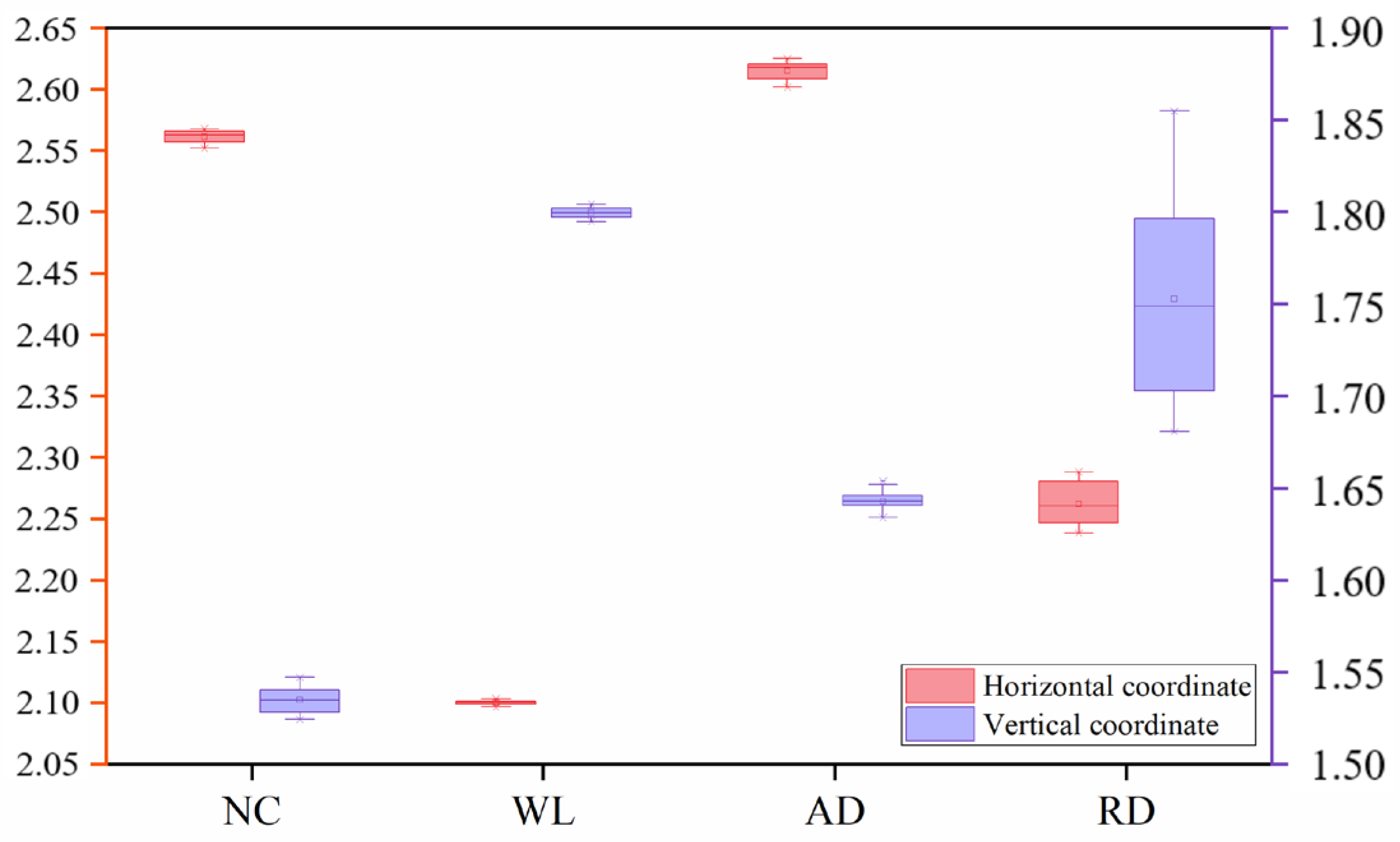
Vibration signals from load test1 are employed to illustrate the centroid features and BCS index, corresponding to the transformer under healthy conditions and typical faults. Figure 11 presents box plots showing the distribution ranges of the horizontal and vertical coordinates of the vibration centroids across the four conditions of transformer winding. As can be seen from the figure, the ranges of the centroid coordinates differ substantially across the various winding conditions. Specifically, when transformer winding is loose, the horizontal coordinate of the vibration centroid exhibits a remarkably confined variation range, spanning only from 2.097 to 2.104. In contrast, when radial deformation of the transformer winding occurs, the variations for both horizontal and vertical coordinates are the largest among the four winding conditions. Among them, the horizontal coordinate varies from 2.23 to 2.29, and the vertical coordinate ranges from 1.68 to 1.85.

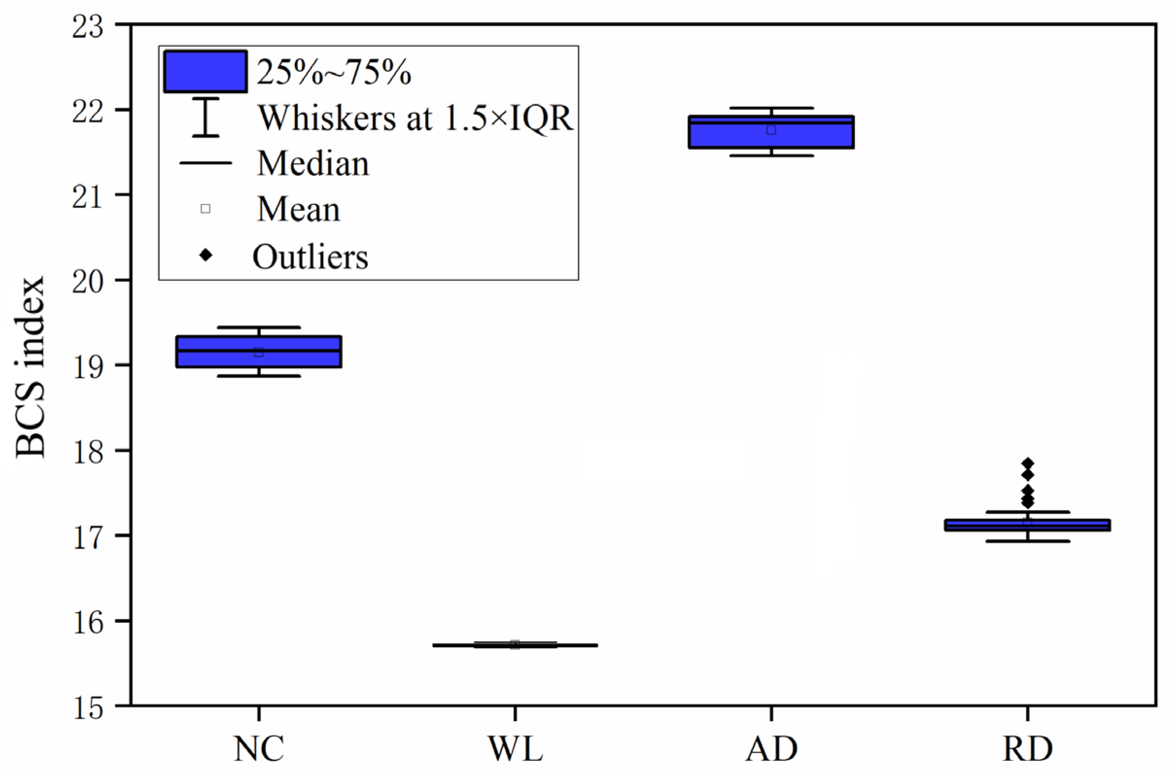
The box plots showing the distribution ranges of the BCS index across the four winding conditions are shown in Figure 12. As can be seen from the figure, the BCS index, as a metric that integrates the horizontal and vertical coordinate information of the vibration centroid, demonstrates notable consistency with the distribution features of the centroid coordinates themselves. Specifically, the BCS index ranges from 18.86 to 19.44 for a healthy transformer winding. When a transformer winding is loose, the BCS index demonstrates the narrowest variation, restricted to an interval of 15.68 to 15.76. In the case of axial deformation of a transformer winding, the BCS index varies between 21.45 and 22.02. Notably, the largest variation is observed during radial deformation, with the BCS index ranging from 16.93 to 17.72. Moreover, a portion of the data lies beyond 1.5 times the interquartile range (IQR), indicating a relatively higher degree of dispersion in the BCS index for radial deformation of transformer winding.

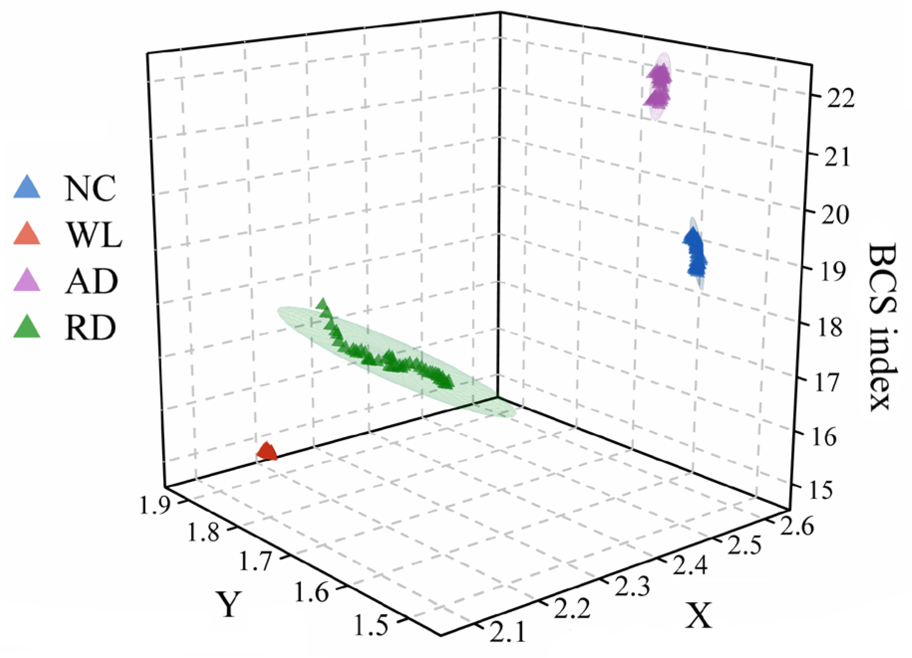
Figure 13 illustrates the spatial distribution diagram of the proposed feature vectors for fault diagnosis, which is composed of the horizontal coordinate of the vibration centroid, the vertical coordinate of the vibration centroid, and the BCS index. In the figure, the elliptical spheres represent the 95% confidence intervals for the spatial points across the four winding conditions. As can be seen from the figure, the spatial points formed by the proposed feature parameters in three-dimensional space exhibit distinct distribution patterns across different winding conditions. Specifically, the spatial clusters for the healthy condition and axial deformation of transformer winding are relatively proximate along the horizontal coordinate and occupy similar volumetric ranges, as indicated by their confidence ellipsoids of comparable size. In contrast, the cluster for the winding looseness demonstrates high spatial concentration, whereas the points representing the radial deformation show significantly greater dispersion. Apparently, the confidence ellipsoids for each winding condition demonstrate no overlap, providing definitive visual and statistical evidence that the proposed feature vectors are substantially distinct across different conditions of transformer winding. This clear separability confirms that the feature set satisfactorily meets the requirement for accurate and reliable condition identification of transformer winding.

4.2. Performance of GWO-LSSVM-Based Classifier

The measured vibration signals under the four winding conditions were segmented to calculate the feature vectors, facilitating the dataset construction and fault diagnosis. Each feature vector is composed of the horizontal coordinate of the vibration centroid, the vertical coordinate of the vibration centroid, and the BCS index. A total of 256 samples were obtained and randomly divided into a training set and a test set. On the training set, a GWO-LSSVM classifier was developed. Specifically, a 5-fold cross-validation incorporated with the GWO algorithm was adopted to optimize the hyperparameters of the LSSVM and then train the classifier. Subsequently, the remaining 64 test samples were used to evaluate the diagnostic performance of the trained classifier.

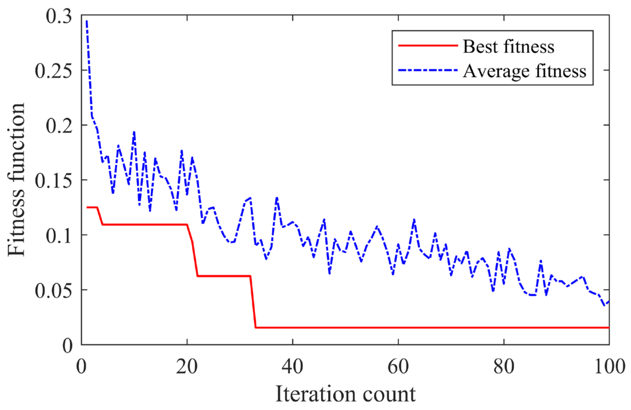
The hyperparameters of the penalty factor and the bandwidth of the kernel function in the GWO-LSSVM-based classifier were determined, and the iteration curve was illustrated in Figure 14. Here, the parameter ranges for the penalty factor and the bandwidth were set as [0.01, 1000] and [0.01, 100], respectively. The size of the wolf pack was set to 20, with a maximum iteration count of 100. The fitness function of the GWO was the misclassification rate. As can be seen from the figure, the fitness curve shows a downward trend, stabilizing at the 32nd iteration as the iteration process progresses. The optimal parameters for the penalty factor and the bandwidth are thus identified as 677.8580 and 24.3735, respectively.

With the obtained optimal hyperparameters, the well-trained GWO-LSSVM classifier was tested on the test set. To assess the reliability of the proposed method, the following metrics are employed, including accuracy (Ac), precision (Pc), recall (Rc), and F1 score (F1). These metrics are calculated by [19]

Pc = TP/(TP + FP)

(18)

Ac = (TP + TN)/(TP + FP + TN + FN)

(19)

Rc = TP/(TP + FN)

(20)

F1 = 2 × (Rc × Pc)/(Rc + Pc)

(21)

where True Positive (TP) is the number of actual positives correctly predicted as positive, True Negative (TN) is the number of actual negatives correctly predicted as negative, False Positive (FP) refers to the number of actual negatives incorrectly predicted as positive, and False Negative (FN) refers to the number of actual positives incorrectly predicted as negative.

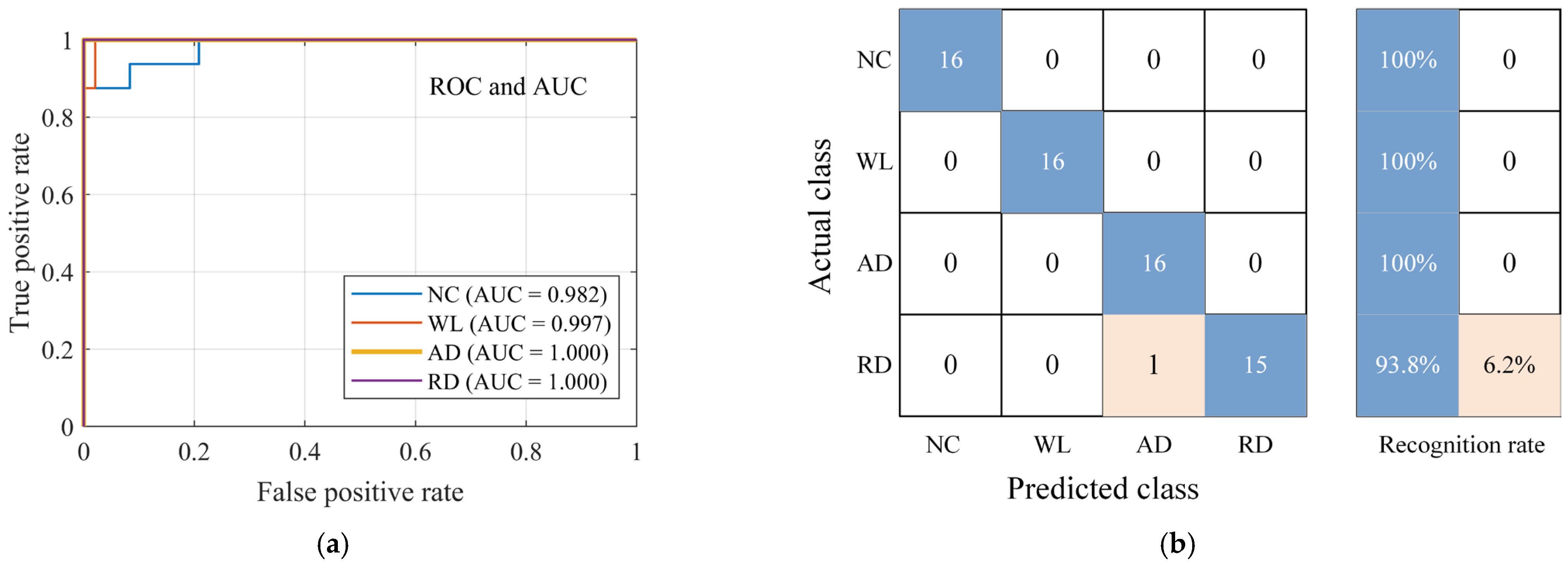
The performance evaluation of the GWO-LSSVM-based classifier is shown in Figure 15. Here, ROC curves for each fault type were generated using a one-versus-rest strategy. As can be seen from the figure, the ROC curves for all four classes rise sharply toward the top-left corner, yielding AUC values of 0.982 for the normal condition of transformer winding, 0.997 for winding deformation, and 1.0 for axial deformation and radial deformation, respectively. These results indicate that the proposed GWO-LSSVM-based classifier achieves excellent discriminative performance across all fault types. Meanwhile, a total of 63 datasets are correctly classified by the GWO-LSSVM-based classifier, achieving an overall recognition accuracy of 98.44%. Specifically, one case of radial deformation is misclassified as axial deformation. The reason for this is partly due to the co-occurrence of radial deformation and axial deformation of transformer winding, and the mixed nature of the vibration source. Indeed, radial deformation and axial deformation would modify the radial stiffness and axial stiffness of transformer winding, respectively, thus theoretically altering its radial vibration mode and axial stiffness. However, influenced by the strong coupling of the electromagnetic structure of transformer winding, radial deformation often induces local tilting of the winding disks, introducing an axial deformation component, and vice versa. Meanwhile, vibration signals on the transformer tank are inherently spatially and modally mixed, containing contributions from electromagnetic interactions and structural response that are simultaneously influenced by both axial and radial stiffness changes. Hence, it is sometimes difficult to distinguish the axial and radial deformation that exhibits similar characteristics. In this paper, the authors propose a discriminative feature vector by integrating the coordinates of the vibration centroid with the BCS index. This approach maps the one-dimensional spectral data of vibration signals into a two-dimensional spatial morphology, offering a novel approach to enhance the identification of winding deformation. The obtained classification results successfully validate the effectiveness of the proposed method.

4.3. Comparisons

This section presents comparisons to validate the effectiveness of the proposed method, including feature vectors, the optimized algorithm, and different small-sample classifiers. Detailed descriptions are as follows.

4.3.1. Feature Vectors of Vibration Signals

To verify the effectiveness of the proposed spatial-based feature vectors for vibration signals, a dataset was constructed from four winding conditions, consisting of the amplitude at the fundamental frequency of vibration signals, measured during the load test1. The GWO-LSSVM-based classifier was trained, and the recognition accuracy for the test set was illustrated in

Table 4. Recognition accuracy of the GWO-LSSVM-based classifier with different feature vectors.

Number of Vibration Sensor	Feature Vector	Average Accuracy/%
No.3	Amplitude at fundamental frequency	87.47
No.6	Amplitude at fundamental frequency	85.32
No.3 and No.6	Majority voting	92.80
No.3~No.6	Coordinate of vibration centroid and BCS index	95.31
No.1~No.6	Coordinate of vibration centroid and BCS index	98.44

. Since the winding faults are simulated on the phase C winding, vibration signals from accelerometers No.3 and No.6 were analyzed, respectively, where the amplitude of the fundamental frequency component was selected as a feature parameter. Meanwhile, based on the results derived from two separate GWO-LSSVM-based classifiers, corresponding to accelerometers No.3 and No.6, majority voting was employed to reach the final decision for classification. The robustness of the proposed method against accelerometer failure was further evaluated, where accelerometers No.1 and No.2 were strategically excluded from the full six-accelerometer array. As can be observed in the table, the recognition accuracy of the proposed method is significantly higher than the other four cases, where vibration signals from a single location of the transformer tank are considered, the fusion through majority voting, as well as the accelerometer failure. This indicates the effectiveness of the constructed feature vectors of vibration signals, since it comprehensively incorporates vibration response from several locations on the transformer tank. Notably, even under the failure of two accelerometers (e.g., No.1 and No.2) on the transformer tank, the identification accuracy of the proposed method exhibits only a modest reduction, from 98.44% to 95.31%.

Meanwhile, the proposed feature vectors were compared with other established feature extraction methods, including the statistical features from [16] and the EWT from [21]. Specifically, following [16], the main fundamental vibration ratio and vibration entropy of vibration signals were computed, and the EWT was applied following [21] to decompose the vibration signals to obtain multiscale entropy for all selected EWF components for dataset construction. Based on the constructed dataset, the GWO-LSSVM-based classifier was trained, and the recognition accuracy for the test set was illustrated in

Table 5. Comparisons of GWO-LSSVM-based classifier with established feature extraction methods.

Established Feature Extraction Methods	Feature Parameters	Average Accuracy (%)	Training Time (s)
EWT	Multiscale entropy for all selected EWF components	93.75	2.67
Statistical Features	Vibration main fundamental Ratio and vibration entropy	90.63	1.82
This Paper	BCS index	98.44	2.04

. As can be observed from the table, the proposed method achieves an average accuracy that is 4.69% higher than that of EWT and 7.81% higher than that of statistical features. We attribute this superiority to the strong feature discriminative ability of the proposed feature vectors. When the transformer winding transitions from normal to deformation, both the vibration pattern and the vibration propagation path are changed, leading to a redistribution of vibration energy. The defined feature vectors, consisting of the distribution of the vibration centroid and the BCS index, are capable of capturing these variations in the acquired vibration signals. Nevertheless, it is worth noting that features extracted individually from multiple accelerometers (e.g., the six accelerometers employed in this study) focus on vibration intensity or energy. This approach not only introduces redundant information but, more importantly, fails to adequately fuse spatial correlations, thereby impairing the performance of the diagnostic model to some extent.

4.3.2. Optimized Methods for LSSVM-Based Classifier

The optimized methods, namely particle swarm optimization (PSO) and a genetic algorithm (GA), are employed to optimize the hyperparameters in the LSSVM-based classifier. A 5-fold cross-validation was conducted. This process was repeated with ten different random seeds to ensure diverse data splits. The experiment was independently performed for all three classifiers, namely GWO-LSSVM, PSO-LSSVM, and GA-LSSVM. As summarized in

Table 6. Comparisons of the GWO-LSSVM-based classifier with different optimization algorithms.

Classifiers	GWO-LSSVM	PSO-LSSVM	GA-LSSVM
Average Accuracy (%)	98.44% ± 1.48%	89.08% ± 1.50%	95.33%± 1.92%

, the proposed GWO-LSSVM achieved a mean classification accuracy of 98.44% with a standard deviation of ±1.48% across the five folds. In comparison, PSO-LSSVM and GA-LSSVM yielded mean accuracies of 89.08% ± 1.50% and 95.33% ± 1.92%, respectively. Notably, the standard deviation intervals of GWO-LSSVM (96.96–99.92%) do not overlap with those of PSO-LSSVM or GA-LSSVM (89.3–92.3%), indicating that the performance advantage of GWO is consistent across different data splits and is unlikely to arise from random variation. Meanwhile, GA and PSO converged in an average of 38 and 46 iterations, respectively. It should be noted that the convergence reported herein refers to the optimal solution achieved by each algorithm after completing its respective iterative search, rather than implying iteration counts across algorithms. These results demonstrate that the GWO-optimized LSSVM not only achieves higher diagnostic accuracy but also exhibits superior stability, generalization, and optimization efficiency compared to PSO and GA under the same feature extraction and classification framework.

4.3.3. Different Classifiers

To evaluate the performance of the GWO-LSSVM-based classifier, several classifiers, including the SVM, LSSVM, Backpropagation Neural Network (BPNN), k-Nearest Neighbor (KNN), Sparse Bayesian ELM (SBELM), RF, XGBoost, and 1D-CNN, were selected for comparisons. Among them, several of these classifiers have been employed in the literature to diagnose winding faults. Based on the same dataset, the evaluation indices corresponding to the different classifiers are shown in

Table 7. Metrics for the different classifiers.

Classifiers	Ac	Pc	Re	F1	Time Loss (s)
GWO-LSSVM	0.9844	0.9853	0.9844	0.9844	1.84
LSSVM	0.7500	0.8643	0.7500	0.6840	0.25
SVM	0.8281	0.8681	0.8281	0.8128	1.22
BPNN	0.5000	0.3387	0.5000	0.6738	2.19
KNN	0.7500	0.8333	0.7500	0.8889	0.41
SBELM	0.5781	0.5038	0.5781	0.7059	0.17
RF	0.8281	0.8706	0.8281	0.8197	1.17
XGBoost	0.8475	0.8512	0.8475	0.8669	1.03
1D-CNN	0.9280	0.9171	0.9280	0.8872	2.26

. As can be seen in the table, the performance of the classifiers can be ordered as follows: GWO-LSSVM > 1D-CNN > XGBoost > RF > SVM > LSSVM > KNN > SBELM > BPNN. Among the seven different models, the proposed model reaches a 98.44% accuracy, despite its slightly increased computational time. This computation burden stems from the iterative hyperparameter search process, which generally involves N_t × N_p iterations, where N_t is the number of iterations and N_p is the wolf population size. Notably, the GWO-LSSVM classifier exhibits fast convergence throughout the iterative process, and the extra computational cost is incurred exclusively during the offline training phase. Hence, this trade-off between computational overhead and diagnostic accuracy is considered acceptable for fault diagnosis in transformer winding. In contrast, the less time-consuming models, including LSSVM, KNN, and SBELM, exhibited lower classification accuracy. Both XGBoost and RF attain an accuracy of 82%, but the time loss of RF is slightly less than that of XGBoost. The 1D-CNN achieves a higher accuracy of 92.8%, with a computational time of 2.26 s. Evidently, the performance of these classifiers does not yet meet the desired standards. The proposed model in the paper can realize winding fault detection with high accuracy.

5. Discussions

This study presents a vibration centroid-based method for diagnosing winding faults of a transformer. The key finding is that the proposed feature vectors, combined with a GWO-LSSVM classifier, achieve 98.44% accuracy in identifying normal, winding looseness, axial deformation, and radial deformation. Although experimental validation is limited to a single 35 kV-rated transformer under laboratory conditions, the proposed method is not inherently confined to this specific rating. The core feature vectors, namely the distribution of vibration centroid and the BCS index, capture both the fundamental frequency component and the spatial pattern across multiple accelerators. These features inherently reflect the mechanical response of the winding-core system to electromagnetic excitation, a response governed by fundamental principles of vibration mechanics and magnetostriction that apply across transformer designs and voltage classes. Similarly, the GWO-LSSVM classifier operates on feature vectors, making it insensitive to absolute signal amplitudes that may vary across different units. Hence, this method is theoretically design-independent and should be transferable. However, several factors must be acknowledged as potential influences on the diagnostic performance of the proposed method, including load current; the mechanical structure of the transformer winding, core, and tank; the operating environment of the transformer; and the placement of accelerometers on the tank surface. To further demonstrate the diagnostic model’s performance, the effect of load current and the placement of accelerometers on the GWO-LSSVM-based classifier, as well as the model’s robustness, were investigated.

5.1. Effect of Load Currents

The load current of an operating transformer always fluctuates in response to load demand. These variations directly affect the electromagnetic forces acting on the windings, which in turn alter the vibration signals on the transformer tank. Despite the inherent advantage of the BCS index in accommodating vibration signal variations induced by different load currents or sensor placement changes, the influence of fluctuating load currents on the diagnostic performance of different transformers remains inevitable. To analyze the effect of load currents on classification, a dataset was constructed from four winding conditions, consisting of the coordinates of the vibration centroid and the BCS index of vibration signals, measured during the load test1, load test2 and short-circuit test.

Table 8. Average accuracy of different classifiers at different load currents.

Classifiers	Load Test 1	Load Test 2	Short-Circuit Test
GWO-LSSVM	0.9844	0.9531	1.00
LSSVM	0.7500	0.7344	0.8750
SVM	0.8281	0.7967	0.9063
BPNN	0.5000	0.5000	0.8281
KNN	0.7500	0.7344	0.8594
SBELM	0.5781	0.5781	0.8438
RF	0.8281	0.8125	0.9219
XGBoost	0.8475	0.8438	0.9280
1D-CNN	0.9063	0.8594	0.9375

shows the average accuracy of different classifiers at different load currents. As can be observed, the classification performance of the eight kinds of classifiers depends on the load current to a certain degree. Specifically, higher accuracy is achieved at the current during the short-circuit test. At the highest point, the corresponding current is the rated current. The accuracy of all classifiers decreases at the lower currents, partly because the vibration signal is weaker, whose quality is further compromised by the core vibration. However, the proposed method achieves the higher average accuracy, since the BCS index exhibits inherent invariance to scaling and rotation, which partially mitigates the effect of current-induced amplitude variations.

5.2. Effect of the Placement of Accelerations

Due to the mechanical structure of the transformer and the measurement errors, it is always difficult to ensure that the placement of accelerometers on the transformer tank remains invariant, even for the same transformer. Consequently, these placement variations would exert a non-negligible influence on the performance of the proposed GWO-LSSVM classifier. To simulate this effect, perturbation analysis was conducted on the proposed feature vectors derived from the vibration signals. Specifically, the values of feature vectors in the test set were randomly scaled within a range of ±5% to ±10% of their original values, mimicking the potential deviations that may be caused by the repositioning of accelerometers on the transformer tank. Here, the selected perturbation range was chosen to cover practical uncertainties in the acquisition of vibration signals, including positional variation in accelerometers and local structural differences in the transformer tank. Still taking the feature vectors obtained from load test1 as an illustrative example, the corresponding results of this analysis are summarized in

Table 9. Metrics of the GWO-LSSVM-based classifier at different placements of accelerometers.

Varied Range of Feature Vectors	−10%	−5%	0	5%	10%
Ac	0.9219	0.9531	0.9844	0.9688	0.9062
Pc	0.9280	0.9605	0.9853	0.9806	0.9196
Re	0.9219	0.9531	0.9844	0.9688	0.9062
F1	0.9215	0.9527	0.9844	0.9687	0.9046

. As can be seen from the table, at the maximum perturbation level of ±10%, the diagnostic accuracy remained above 90%, indicating that the proposed method exhibits robustness to amplitude variations arising from sensor placement changes within a certain range.

5.3. Robustness Analysis

When acquiring vibration signals from the transformer tank, the effect of noise is always inevitable. To assess the noise effect on the performance of the GWO-LSSVM classifier, white Gaussian noise was artificially added to the original signals at five signal-to-noise (SNR) levels: 5 dB, 10 dB, 20 dB, 25 dB, and 30 dB. These levels were selected to cover typical conditions in the field as well as extreme scenarios. Still taking the vibration signal obtained from load test1 as an illustrative example. The corresponding results of this analysis are summarized in

Table 10. Average accuracy of GWO-LSSVM at different noise levels.

SNR	5 dB	10 dB	20 dB	25 B	30 dB
Average Accuracy	0.9844	0.9844	0.9844	0.9844	0.9531
Training Time (s)	2.04	2.04	2.07	2.10	2.14

. As can be seen from the table, the diagnostic accuracy under 30 dB noise was 95.31%, compared to 98.44% under noise-free conditions, representing a degradation of only 3.13%. Furthermore, the training time was prolonged, as the presence of noise introduces additional uncertainty into the training process of the GWO-LSSVM-based classifier. Despite this, the proposed method exhibits strong noise robustness, largely attributable to the inherent invariance of the BCS index to scaling and common-mode perturbations.

5.4. Suggestions and Limitations

For the operating transformers in the field, where load current inevitably fluctuates, the following three practical recommendations are suggested. The first recommendation is to incorporate load current directly into the feature vectors or, alternatively, to apply a current-based compensation factor to the extracted feature vectors. The second recommendation is to prioritize the measurement and diagnosis of vibration signals under high load ratios, where the fault-related features embedded in the vibration signals become more discernible. The third recommendation involves the placement of accelerometers on the transformer tank. Specifically, accelerometers should be positioned at approximately one-quarter and three-quarters of the winding height from the upper tank edge, with care taken to avoid the stiffeners of the transformer tank. In addition, the position of each accelerometer on a given transformer should remain as consistent as possible over time, and a minimum of six accelerometers is recommended for reliable acquisition of the vibration signals.

In this paper, three kinds of winding faults, namely winding looseness, axial deformation, and radial deformation, were simulated and identified. These faults were always caused by either a single severe short-circuit impact or the cumulative effect of multiple milder short-circuit impacts on the transformer winding. Although each short-circuit event is extremely short (typically <2 s) and often treated as an adiabatic process, the instantaneous temperature rise can reach several hundred degrees Celsius. Each such thermal impact causes thermal degradation of the cellulose insulation–primarily pyrolysis and a reduction in the degree of polymerization. After multiple short-circuit impacts, the mechanical strength of the insulation gradually deteriorates, eventually leading to catastrophic failure during a subsequent short-circuit event. Hence, the conclusions of this study are primarily applicable to single-event fault diagnosis or end-state damage assessment. However, the thermal-mechanical damage of actual short-circuit impacts is also a major concern in transformer life management, and validation under repeated short-circuit shocks is an important direction for future work.

6. Conclusions

Aimed to precisely and efficiently identify winding faults, this paper presents a GWO-LSSVM-based classifier integrated with a new spatial vibration feature vector. Based on the theoretical analysis of transformer vibration and the strategic layout of vibration accelerometers mounted on the transformer tank, the Zoom-FFT technique was employed to obtain the frequency spectrum of vibration signals, achieving a significant improvement in both frequency resolution and amplitude accuracy. The distribution of the vibration centroid and the BCS index were defined to construct the vibration feature vectors. This approach incorporates both frequency spectrum and spatial dimensions, as well as the shape index, thereby achieving a more comprehensive description of winding condition through the derived feature parameters. On this basis, the GWO-LSSVM-based classifier was developed to identify the winding faults, where the hyperparameters, namely penalty factor and bandwidth of the kernel function, were optimized by the GWO algorithm to achieve optimal classification accuracy and strong generalization. Benefiting from its efficiency and small-sample performance, this approach is particularly well-suited for fault diagnosis of transformer winding in resource-constrained environments. No-load, short-circuit, and load tests were conducted on a 35 kV-rated oil-immersed transformer for verification. During the experiment, transformer winding was divided into four categories that include healthy condition, winding looseness, axial deformation, and radial deformation. The results show that the proposed method achieved an overall recognition rate of 98.44% on a balanced dataset of 256 samples covering four winding conditions. A comprehensive comparison and discussion across feature vectors, optimization algorithms, classifiers, load currents, and noise further demonstrate the effectiveness of the proposed approach.

While the proposed method demonstrates strong performance under controlled conditions and known winding faults, its generalization to operational transformers under fluctuating load currents, diverse transformer types, and complicated fault modes of transformer winding requires further validation. Future work would focus on establishing a dataset encompassing diverse fault scenarios of transformer windings to test and enhance the robustness of the proposed method, covering different voltage levels (e.g., 110 kV, 220 kV), different manufacturers, and field operating conditions including varying temperatures and oil conditions. Meanwhile, this study emphatically focuses on single-event fault diagnosis or end-state damage assessment of a transformer. Validation under genuinely repeated short-circuit impacts with progressive thermal-mechanical degradation is another important direction for future work. As a substantial volume of data continues to accumulate, deep learning and transfer learning will also be explored to further improve the diagnostic accuracy for winding deformation.

References

1. Li, Z.; Cheng, J.; Abu-Siada, A. Classification and Location of Transformer Winding Deformations using Genetic Algorithm and Support Vector Machine. Recent Adv. Electr. Electron. Eng. 2021, 14, 837–845. [Google Scholar] [CrossRef] [Scilit]
2. Mortazavi, M.; Moravej, Z.; Gharehpetian, G.B. Detection and localization of LV winding radial deformation in transformers using electromagnetic waves—A feasibility. Study Int. J. Electr. Power Energy Syst. 2024, 155, 109602. [Google Scholar] [CrossRef] [Scilit]
3. Messadi, A.; Zouaghi, A.; Ferdiallah-kherkhachi, E.; Vollaire, C.; Richer, O.; De Oliveira, L.F.; Breard, A. High frequency model of power transformer bushing for very fast transient studies. IEEE Access 2023, 11, 93908–93919. [Google Scholar] [CrossRef] [Scilit]
4. IEC 60076–5; Power Transformers—Part 5: Ability to Withstand Short Circuit. IEC: Geneva, Switzerland, 2006.
5. Liu, J.; Chen, S.; Wang, F.; Zhu, D.; Li, X.; Zhong, Y.; Li, Z. Experimental investigation on cumulative effects of transformer winding deformation under short-circuit impulses. IET Electr. Power Appl. 2025, 19, e70020. [Google Scholar] [CrossRef] [Scilit]
6. Cao, C.; Xu, J.; Lin, X.; Li, X. State diagnosis method of transformer winding deformation based on fusing vibration and reactance parameters. IET Electr. Power Appl. 2020, 14, 818–826. [Google Scholar] [CrossRef] [Scilit]
7. Shamlou, A.; Feyzi, M.R.; Behjat, V. Winding deformation classification in a power transformer based on the time-frequency image of frequency response analysis using Hilbert-Huang transform and evidence theory. Int. J. Electr. Power Energy Syst. 2021, 129, 106854. [Google Scholar] [CrossRef] [Scilit]
8. Thango, B.A. Six sigma-based frequency response analysis for power transformer winding deformation. Appl. Sci. 2025, 15, 3951. [Google Scholar] [CrossRef] [Scilit]
9. Asl, M.B.; Fofana, I.; Meghnefi, F.; Brahami, Y.; Da Costa Souza, J.P. A comprehensive review of transformer winding diagnostics: Integrating frequency response analysis with machine learning approaches. Energies 2025, 18, 1290. [Google Scholar] [CrossRef] [Scilit]
10. Guobin, W.; Kang, W.; Xiaolin, X.; Guangyu, S.; Yu, L.; Shengwen, S. Transformer winding deformation diagnosis method based on dynamic time warping and multilayer perceptron. Front. Energy Res. 2025, 13, 1731410. [Google Scholar] [CrossRef] [Scilit]
11. Wang, S.; Wang, S.; Cui, Y.; Long, J.; Ren, F.; Ji, S.; Wang, S. An experimental study of the sweep frequency impedance method on the winding deformation of an onsite power transformer. Energies 2020, 13, 3511. [Google Scholar] [CrossRef] [Scilit]
12. Zhao, X.; Yao, C.; Zhang, C.; Abu-Siada, A. Toward reliable interpretation of power transformer sweep frequency impedance signatures: Experimental analysis. IEEE Electr. Insul. Mag. 2018, 34, 40–51. [Google Scholar] [CrossRef]
13. Seifaddini, N.; Sekongo, B.; Fofana, I.; Akre, S.; Chehri, A.; Ouhrouche, M. Towards winding deformation assessment from vibration signals using an optical sensor. IET Sci. Meas. Technol. 2024, 19, e12224. [Google Scholar] [CrossRef] [Scilit]
14. Akre, S.; Fofana, I.; Yeo, Z.; Brettschneider, S.; Kung, P.; Sékongo, B. On the feasibility of monitoring power transformer’s winding vibration and temperature along with moisture in oil using optical sensors. Sensors 2023, 23, 2310. [Google Scholar] [CrossRef] [Scilit] [PubMed]
15. Nezhad, A.E.; Samimi, M.H. Investigation of transformer vibration characteristics using the finite element method. Sci. Iran. 2024, 31, 441–457. [Google Scholar]
16. Liu, J.; Chen, S.; Wang, F.; Zhu, D.; Xu, K.; Chen, P.; Li, J.; Li, Z. Theoretical evaluation of transformer short-circuit withstand capability and identification method of winding cumulative deformation. IEEE Trans. Power Deliv. 2025, 40, 2454–2465. [Google Scholar] [CrossRef] [Scilit]
17. Wang, N.; Zheng, J.; Yuan, Y. Vibration model of ±800kV converter transformers under varying load conditions. Energies 2025, 18, 5968. [Google Scholar] [CrossRef] [Scilit]
18. Pallot, J.; Exanayake, C.; Ma, H.; Naranpanawe, L. Application of operational modal analysis to investigate transformer vibration patterns. IET Gener. Transm. Distrib. 2022, 16, 1964–1973. [Google Scholar] [CrossRef] [Scilit]
19. Sun, Y.; Ma, H. Interpretable analysis of transformer winding vibration characteristics: SHAP and multi-classification feature optimization. Int. J. Electr. Power Energy Syst. 2025, 166, 110582. [Google Scholar] [CrossRef] [Scilit]
20. Rao, S.; Nie, S.; Lv, X.; Ruan, W.; Yin, F.; Barmada, S.; Zhao, Y.; Deng, Y. Evaluating power transformer state based on tank vibration: A graphical approach. IEEE Trans. Instrum. Meas. 2025, 74, 3539615. [Google Scholar] [CrossRef] [Scilit]
21. Zhao, M.; Xu, G. Feature extraction of power transformer vibration signals based on empirical wavelet transform and multiscale entropy. IET Sci. Meas. Technol. 2018, 12, 63–71. [Google Scholar] [CrossRef] [Scilit]
22. Asl, M.B.; Fofana, I.; Meghnefi, F.; Brahami, Y. Hybrid physics-machine learning diagnostics of transformer winding deformations using FBG sensor. Electr. Power Syst. Res. 2026, 256, 112940. [Google Scholar] [CrossRef] [Scilit]
23. Wang, J.; Guo, J. Application of improved symplectic geometry mode decomposition algorithm in evaluation system of transformer winding short-circuit withstand ability. IEEJ Trans. Electr. Electron. Eng. 2021, 16, 1310–1318. [Google Scholar] [CrossRef] [Scilit]
24. Gao, S.; Sun, L.; Wang, X.; Tian, Y.; Geng, J.; Liu, H. Quantitative research on accumulative effect of transformer winding deformation and its influence degree based on time-frequency analysis of vibration signal. IEEE Access 2022, 10, 133451–133460. [Google Scholar] [CrossRef] [Scilit]
25. Hong, K.; Pan, J.; Jin, M. Transformer condition monitoring based on load-varied vibration response and gru neural network. IEEE Access 2020, 8, 178685–178694. [Google Scholar] [CrossRef] [Scilit]
26. Hong, K.; Jin, M.; Huang, H. Transformer winding fault diagnosis using vibration image and deep learning. IEEE Trans. Power Deliv. 2021, 36, 676–685. [Google Scholar] [CrossRef] [Scilit]
27. Zollanvari, A.; Kunanbayev, K.; Bitaghsir, S.A.; Bagheri, M. Transformer fault prognosis using deep recurrent neural network over vibration signals. IEEE Trans. Instrum. Meas. 2020, 70, 2502011. [Google Scholar] [CrossRef] [Scilit]
28. Xing, Z.; He, Y.; Wang, X.; Chen, J.; Du, B.; He, L.; Liu, X. Vibration-signal-based deep noisy filtering model for online transformer diagnosis. IEEE Trans. Ind. Inform. 2023, 19, 11239–11251. [Google Scholar] [CrossRef] [Scilit]
29. Zhou, Y.; He, Y.; Xing, Z.; Wang, L.; Shao, K.; Lei, L.; Li, Z. Vibration signal-based fusion residual attention model for power transformer fault diagnosis. IEEE Sens. J. 2024, 24, 17231–17242. [Google Scholar] [CrossRef] [Scilit]
30. Fang, J.; Deng, X.; Xia, Y.; Wu, C.; Li, Y.; Li, X.; Chen, K.; Wang, F.; Zhang, Z. Research on identification method of transformer windings’ loose vibration spectrum considering a multi-load current condition. Appl. Sci. 2025, 15, 6949. [Google Scholar] [CrossRef] [Scilit]
31. Wu, M.; Li, C.; Feng, X.; Chen, F.; Feng, Y.; Song, H.; Wang, W.; Zhang, F. Memory-fused dual-stream fault diagnosis network based on transformer vibration signals. SDHM Struct. Durab. Health Monit. 2025, 19, 1473–1487. [Google Scholar] [CrossRef] [Scilit]
32. Wang, F.; Gao, P.; Xue, B.; Zhang, C.; Zhang, L.; Liu, C. A Vibration Response Analysis Technique for Condition Monitoring of Transformer Winding. Appl. Sci. 2026, 16, 6175. [Google Scholar] [CrossRef] [Scilit]
Figure 1. Illustration of a 35 kV oil-immersed three-phase transformer in a power distribution system.
Energies 19 03329 g001
Figure 2. Time-domain waveforms of vibration acceleration of transformer winding at different positions and the corresponding frequency spectra [32]. (a) At the 1/4 position; (b) at the 3/4 position; (c) frequency spectrum.
Energies 19 03329 g002
Figure 3. Schematic diagram of piezoelectric accelerometers on transformer tank. (a) Schematic diagram of piezoelectric accelerometers on transformer tank; (b) real picture of experimental transformer and signal acquisition system.
Energies 19 03329 g003
Figure 4. Real pictures of pre-setting the different winding faults. (a) Winding looseness; (b) axial deformation; (c) radial deformation.
Energies 19 03329 g004
Figure 5. Vibration amplitude at the fundamental frequency, measured across all accelerometers during the no-load, short-circuit, and load tests for a healthy winding.
Energies 19 03329 g005
Figure 6. Frequency spectra of vibration signals measured at accelerometers No.3 and No.6 during load test1 for a healthy winding.
Energies 19 03329 g006
Figure 7. Frequency spectra of vibration signals measured at accelerometer No.3 during the short-circuit test, load test1 and load test2 for a healthy winding.
Energies 19 03329 g007
Figure 8. Frequency spectra of vibration signals measured at accelerometer No.3 during load test1 for different winding faults.
Energies 19 03329 g008
Figure 9. The flow chart of the proposed method.
Energies 19 03329 g009
Figure 10. The flow chart for performing spectral analysis using the Zoom-FFT technique.
Energies 19 03329 g010
Figure 11. Distribution of horizontal and vertical coordinates for the vibration centroids across the four winding conditions. The abbreviations used in this figure are defined in the Abbreviations at the end of this manuscript.
Energies 19 03329 g011
Figure 12. Distribution of the BCS index for vibration centroids across the four winding conditions. The abbreviations used in this figure are defined in the Abbreviations at the end of this manuscript.
Energies 19 03329 g012
Figure 13. Spatial distribution of the feature vectors across the four winding conditions. The abbreviations used in this figure are defined in the Abbreviations at the end of this manuscript.
Energies 19 03329 g013
Figure 14. Iteration curves of hyperparameters in GWO-LSSVM-based classifier.
Energies 19 03329 g014
Figure 15. Performance evaluation of the GWO-LSSVM-based classifier. (a) ROC curves. (b) Confusion matrices. The abbreviations used in this figure are defined in the Abbreviations at the end of this manuscript.
Energies 19 03329 g015