Coordinated Frequency Regulation Strategy for Multi-Type Loads in High-Renewable Power Systems

Abstract

With the increasing penetration of renewable energy, frequency stability issues in new-type power systems have become increasingly prominent due to reduced system inertia and weakened primary frequency regulation capability. To address the insufficient frequency response capability of power systems in high-renewable regions, this paper proposes a coordinated multi-type load frequency control strategy based on controllable load damping factors. First, an improved system frequency response model considering renewable penetration is established to analyze the impacts of renewable penetration on maximum frequency deviation, rate of change of frequency (RoCoF), and quasi-steady-state frequency deviation. Subsequently, coordinated frequency control strategies are designed for feeder voltage-sensitive loads, distributed constant power loads, and energy-intensive industrial loads. Finally, an electromagnetic transient simulation model based on an actual Yunnan power grid is established to verify the effectiveness of the proposed method. The results show that increasing renewable penetration deteriorates frequency response by reducing the frequency nadir, increasing RoCoF, and enlarging quasi-steady-state frequency deviation. Under a −0.1 p.u. active power disturbance, the studied grid triggers under-frequency load shedding when renewable penetration exceeds approximately 44% without load-side frequency regulation, whereas the proposed strategy enables the system to satisfy the 49.2 Hz UFLS constraint at 70% renewable penetration, increasing the allowable renewable accommodation level by about 26 percentage points. Economic analysis further indicates that the proposed load-side control has lower regulation cost than renewable curtailment-based frequency support.

1. Introduction

Driven by the continuous advancement of China’s carbon peaking and carbon neutrality goals, as well as the accelerated development of new-type power systems, the installed capacity of renewable energy in China has been expanding rapidly. In particular, Yunnan Province, relying on its abundant hydropower, wind power, and solar energy resources, has gradually formed a clean energy system characterized by the coordinated development of hydropower, wind power, and photovoltaic power. As an important energy base for China’s “West-to-East Power Transmission” strategy, the Yunnan power grid has experienced a continuous increase in the proportion of renewable energy installations in recent years. Under such high renewable energy penetration, power system frequency stability has become increasingly prominent [1].

Traditional power systems mainly rely on the rotational inertia and primary frequency regulation capability of synchronous generators to maintain system frequency stability. However, renewable energy units, such as wind turbines and photovoltaic generators, are mostly connected to the grid through power electronic converters and therefore lack inherent physical synchronous inertia. As renewable energy sources gradually replace conventional synchronous generators, the equivalent inertia level and primary frequency regulation capacity of the system continue to decrease. Under the same active power disturbance, the rate of change of frequency (RoCoF) increases, the frequency nadir decreases, and the risk of under-frequency load shedding rises. These issues have become important factors limiting the further accommodation of renewable energy [2,3].

The Yunnan power grid is characterized by the coexistence of high renewable energy penetration and large-scale energy-intensive industrial loads. On the one hand, Yunnan has abundant renewable energy resources, and its installed renewable energy capacity has been growing rapidly. On the other hand, the province contains a large number of energy-intensive industrial loads, such as electrolytic aluminum loads, which feature large capacity, fast response, and strong continuous operation capability. These characteristics provide a favorable engineering basis for load-side participation in frequency regulation. Meanwhile, flexible load resources, such as inverter air conditioners, electric vehicles, and variable frequency drive loads, are widely distributed on the distribution side and have considerable frequency regulation potential. Therefore, under high renewable energy penetration, fully exploiting demand-side frequency support capability is of great significance for improving system frequency response characteristics and enhancing renewable energy accommodation capacity [4,5].

In recent years, extensive research has been conducted on load frequency control (LFC). Traditional LFC studies have mainly focused on generation-side control, including PID control, robust control, model predictive control (MPC), fractional-order control, and adaptive control methods [6,7,8]. With the continuous increase in renewable energy penetration, the participation of energy storage systems, virtual power plants, and renewable energy stations in frequency regulation has gradually become a research hot spot.

Demand-side resources participating in frequency regulation have also attracted widespread attention. Existing studies have shown that thermostatically controlled loads can provide fast frequency response within a short time scale due to their thermal inertia characteristics [9,10,11]. Some studies have further considered model predictive control, differentiated control, and user comfort constraints to improve load response accuracy and control robustness [12,13]. Meanwhile, research on frequency control of flexible loads such as electric vehicles, inverter air conditioners, and distributed controllable loads has also continued to develop [14]. In terms of industrial loads, energy-intensive loads such as electrolytic aluminum loads are considered to have high engineering application value because of their large regulation capacity and fast response [15].

Recent studies have further emphasized that frequency regulation in renewable-dominated systems requires coordinated use of heterogeneous resources. Energy-storage-based fast frequency response has rapid active power regulation capability, but it is affected by investment cost, cycle life, and energy-duration constraints [16]. Grid-forming renewable converters can provide voltage and frequency support, but their use may require additional converter control capability, reserve margin, and coordination with system operation rules [17]. Source–grid–load–storage coordinated scheduling has also been studied for 100% renewable energy scenarios, showing the importance of combining frequency security constraints with flexible resources [18]. These studies indicate that no single resource type can fully solve the frequency security problem in high-renewable systems at low cost; therefore, coordinated load-side frequency support remains valuable, especially in regions with large industrial loads.

Table 1. Comparison of representative frequency regulation methods and the proposed strategy.

Method	Main Resource	Typical Advantage	Main Limitation
Generation-side LFC	Synchronous units or conventional generators	Mature control structure and high reliability	Reduced regulation capability as synchronous generation is replaced by renewables
Renewable-side synthetic inertia/deloading	Wind/PV converters	Fast support from converter-interfaced resources	Requires control capability and results in wind and PV curtailment
BESS-based fast frequency response	Battery energy storage systems	Fast active power response	High investment cost, degradation, and limited duration
Proposed multi-type load strategy	Flexible loads	Improves system load damping factor	Requires additional equipment

demonstrates the drawbacks of frequency regulation strategies in existing studies. The multi-type load strategy proposed in this paper belongs to demand response strategies. Distinct from conventional strategies, this paper realizes the “flexibilization” of various loads in the power system through a load damping factor controller. This can raise the system load damping coefficient and improve the frequency response characteristics of the power system. Meanwhile, although many studies have investigated frequency security in receiving-end power grids with high renewable energy penetration, relatively few have considered the specific scenario of energy-intensive industrial loads in Yunnan Province.

To address the above issues, this paper takes an actual power grid in Yunnan as the research object and proposes an Multi-Type Load frequency control method for power systems with high renewable energy penetration. First, an improved system frequency response model considering renewable energy penetration is established to quantitatively analyze the influence of renewable energy penetration on system frequency response characteristics. Then, frequency control strategies are designed for feeder voltage-sensitive loads, distributed constant power loads, and energy-intensive industrial loads, respectively, and a coordinated frequency regulation framework for multiple types of loads is constructed. Finally, electromagnetic transient simulation and economic analysis are carried out based on the actual Yunnan power grid to verify the effectiveness of the proposed method in improving system frequency response characteristics and enhancing renewable energy accommodation capacity.

The main contributions of this paper are as follows:

(1)

An improved system frequency response model considering renewable energy penetration is used as a low-order analytical tool to quantify how renewable substitution affects RoCoF, maximum frequency deviation, and quasi-steady-state frequency deviation, and to support the design of controllable load damping factors.

(2)

A Multi-Type Load frequency control method covering feeder voltage-sensitive loads, distributed constant power loads, and energy-intensive industrial loads is proposed.

(3)

A coordinated frequency regulation framework based on the energy-intensive industrial load scenario in Yunnan is constructed, enabling unified coordination of load-side frequency support resources.

(4)

The effectiveness of the proposed method in improving system frequency security and renewable energy accommodation capacity is verified, and its engineering application value is demonstrated from an economic perspective.

2. Study on Frequency Response Characteristics of Power Systems Considering Renewable Energy Penetration

2.1. Power System Frequency Response Model Considering Renewable Energy Penetration

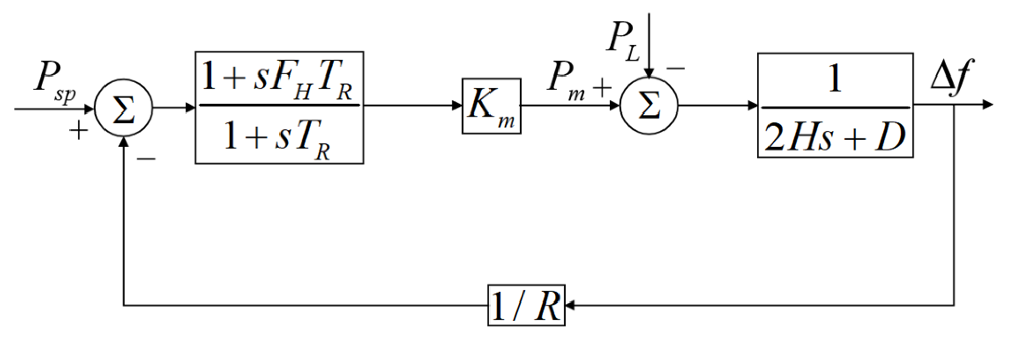
Low-order system frequency response models (SFRMs) are widely used to estimate frequency nadir and dynamic frequency response characteristics after active power disturbances [19]. The frequency response process of the synchronous generator system is summarized as shown in Figure 1.

The block diagram in Figure 1 is obtained from the aggregated swing equation, the load damping relation, the governor droop characteristic, and the reheat turbine dynamic model. In per-unit form, the active power imbalance is balanced by the accelerating power of the equivalent synchronous generator and by frequency-dependent load variation. The governor-turbine path converts frequency deviation into mechanical-power variation through the droop coefficient, turbine gain, high-pressure cylinder coefficient, and reheat time constant. This low-order representation is widely used to evaluate frequency nadir, RoCoF, and quasi-steady-state frequency deviation after a large active power disturbance.

In the figure, Pm is the mechanical power, P_L is the generator electromagnetic power, and Δf is the system frequency deviation, all expressed in per-unit values. In this paper, the power base is defined as the sum of the rated active power of the synchronous generator units that provide physical inertia and conventional primary frequency regulation before the disturbance, while the frequency base is the rated frequency of 50 Hz. F_H is the high-pressure cylinder capacity coefficient of the equivalent reheat turbine, T_R is the equivalent reheat time constant, H is the system equivalent inertia time constant, D is the system load damping factor (LDF), which comprises the generator damping coefficient and the load frequency coefficient, R is the system equivalent regulation coefficient, and Km is the mechanical power gain coefficient, which is a constant related to the system’s active power reserve and power factor.

As thermal power units are gradually replaced by wind and photovoltaic renewable energy units, this paper adopts a conservative modeling assumption that renewable energy sources do not participate in primary frequency regulation. This assumption is used to quantify the frequency security deterioration caused by the loss of synchronous inertia and conventional primary frequency response, and to evaluate the independent contribution of load-side frequency regulation. Although modern wind and PV plants can provide virtual inertia, droop control, or grid-forming frequency support, such functions generally require converter control capability, operational coordination, and in many cases active power reserve or curtailment margin. Since the purpose of this paper is to reduce the dependence on renewable curtailment for frequency support, the no-RES-frequency-support assumption is adopted as a baseline case. Under this assumption, the grid-connected capacity and active power output of thermal power units in the system are (1 − n)S_i and (1 − n)P_i, while the grid-connected capacity and active power output of renewable energy equipment are nS_i and nP_i, where n is the renewable energy penetration rate. The output/capacity ratio of all generating units is equal to the ratio of total active load to total grid-connected capacity of all units, denoted as β. The relationship between the system equivalent inertia time constant H_sys and the synchronous generator inertia time constant H_G is:

$$H_{sys}={\displaystyle \frac{1-n}{\beta }}{H}_G$$

(1)

The system generation-side equivalent power-frequency static characteristic coefficient K_G and the system equivalent regulation coefficient Rsys are related to the synchronous generator regulation coefficient R_G as follows:

$$K_G={\displaystyle \frac{1}{R_{sys}}}={\displaystyle \frac{1-n}{R_G}}$$

(2)

The transfer function of the system is given by

$$G\left(s\right)={\displaystyle \frac{\Delta f}{\Delta P}}={\displaystyle \frac{R_{\mathit{sys}}+R_{sys}{T}_{R}s}{2R_{\mathit{sys}}{H}_{sys}{T}_R{s}^2+\left(2H_{sys}{R}_{\mathit{sys}}+D_{\Sigma }{T}_R{R}_{\mathit{sys}}+K_m{F}_H{T}_R\right)s+D_{\Sigma }{R}_{\mathit{sys}}+K_m}}$$

(3)

where ΔP is the system disturbance power in per-unit value.

Therefore, the relationship between the grid transient frequency deviation and the active power disturbance can be expressed as:

$$\Delta f(t)={\displaystyle \frac{R_{sys}\Delta P}{D_{\sum }{R}_{sys}+K_m}}\left[1+a{e}^{-\varsigma {\omega }_{n}t}\mathit{\text{sin}}\left({\omega }_{r}t+\varphi \right)\right]$$

(4)

The parameters α, ζ, ω_n, ω_r, and ϕ satisfy the following relationships:

$$\alpha =\sqrt{{\displaystyle \frac{1-2T_R\varsigma {\omega }_n+T_R^2{\omega }_n^2}{1-{\varsigma }^2}}}$$

(5)

$$\varsigma =\left({\displaystyle \frac{2H_{sys}{R}_{sys}+\left(D_{\sum }{R}_{sys}+K_m{F}_H\right)T_R}{2\left(D_{\sum }{R}_{sys}+K_m\right)}}\right){\omega }_n$$

(6)

$${\omega }_n=\sqrt{{\displaystyle \frac{D_{\sum }{R}_{sys}+K_m}{2HR{T}_R}}}$$

(7)

$${\omega }_r={\omega }_n\sqrt{1-{\varsigma }^2}$$

(8)

$$\varphi ={\varphi }_1-{\varphi }_2={\mathit{\text{tan}}}^{-1}\left({\displaystyle \frac{{\omega }_r{T}_R}{1-\varsigma {\omega }_n{T}_R}}\right)-{\mathit{\text{tan}}}^{-1}\left({\displaystyle \frac{\sqrt{1-{\varsigma }^2}}{-\varsigma }}\right)$$

(9)

In existing research, according to the temporal sequence of frequency dynamic response, the key indicators describing frequency response characteristics are as follows. (1) Initial rate of change of frequency RoCoF(0): the speed of frequency change in the initial period after the disturbance. Since the frequency change speed always achieves its maximum value at the initial moment after the disturbance, RoCoF(0) can also be recorded as the maximum rate of change of frequency RoCoF_max. (2) Maximum frequency deviation Δf_max: the maximum or minimum value of frequency during the dynamic process. In a receiving-end system, if the frequency nadir falls below the under-frequency load shedding threshold, it will trigger under-frequency load shedding and cause large-scale blackouts. The under-frequency load shedding threshold in Yunnan Province, China, is 49.2 Hz. (3) Quasi-steady-state frequency deviation Δf_ss: the steady-state value reached after the frequency dynamic process stabilizes.

According to Equation (4), setting t = ∞ yields the quasi-steady-state frequency deviation after the disturbance:

$$\Delta f_{ss}={\displaystyle \frac{R_{sys}\Delta P}{D_{\sum }{R}_{sys}+K_m}}$$

(10)

Taking the derivative of Equation (4), the time-varying law of the power system RoCoF is obtained as:

$$RoCoF(t)={\displaystyle \frac{d\Delta \omega (t)}{dt}}=a{\omega }_n{\displaystyle \frac{R\Delta P}{D_{\sum }R+K_m}}{e}^{-\varsigma {\omega }_{n}t}\sin \left({\omega }_{r}t+{\varphi }_1\right)$$

(11)

The maximum value of the power system RoCoF, i.e., the initial value, is:

$$RoCo{F}_{\max }=RoCoF\left(0\right)={\displaystyle \frac{d\Delta \omega (t)}{dt}}=a{\omega }_n{\displaystyle \frac{R_{sys}\Delta P}{D_{\sum }{R}_{sys}+K_m}}\sin \left({\varphi }_1\right)={\displaystyle \frac{\Delta P}{2H_{sys}}}$$

(12)

In practical applications, the RoCoF over a certain short period (t1 − t2) after the disturbance is usually examined, namely:

$$RoCo{F}_{\mathrm{e}}={\displaystyle \frac{\omega (t_1+t_2)-\omega (t_1)}{t_2-t_1}}$$

(13)

where RoCoFc is the assessed value of the RoCoF. In this paper, the system RoCoF within the first 0.3 s after the disturbance occurrence is taken as the assessed value of the initial RoCoF.

Setting RoCoF(t_z) = 0 yields:

$$t_z={\displaystyle \frac{-{\varphi }_1}{{\omega }_r}}$$

(14)

where t_z is the time at which the extremum is reached. The frequency deviation extremum is calculated as:

$$\Delta f_{\mathit{max}}={\displaystyle \frac{R_{sys}\Delta P}{D_{\sum }{R}_{sys}+K_m}}\left[1+a{e}^{-\varsigma {\omega }_n{t}_z}\sqrt{1-{\varsigma }^2}\right]$$

(15)

2.2. Analysis of the Impact of Increasing Renewable Energy Penetration on System Frequency Response Characteristics

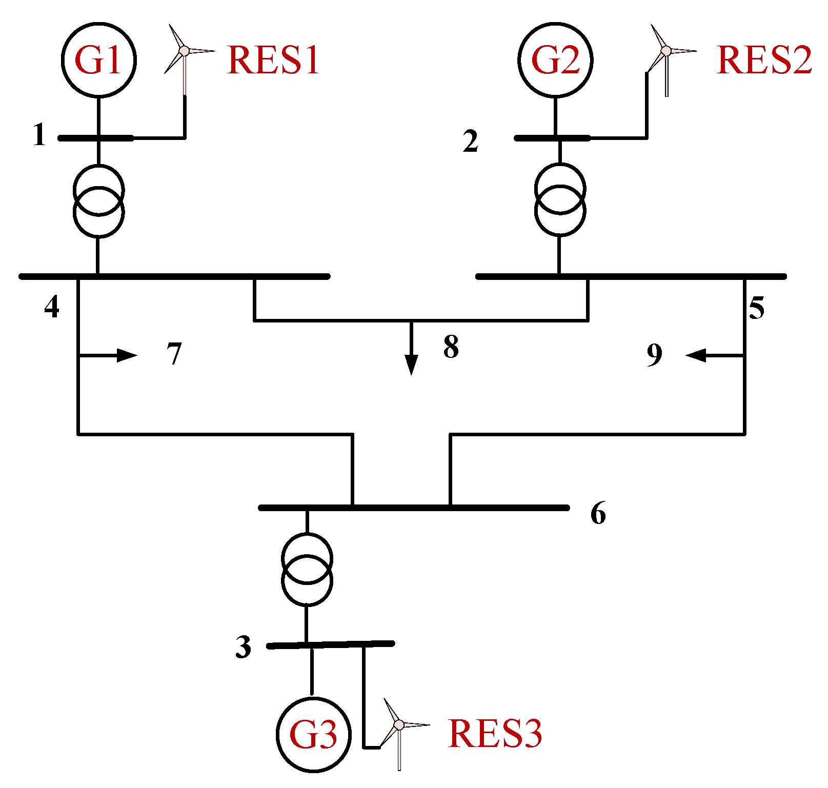
To verify the effectiveness of the ISFRM, modifications are made on the basis of the IEEE nine-bus topology to obtain the three-machine nine-bus topology shown in Figure 2. Conventional generators G1–G3 are connected to buses 1, 2, and 3, respectively. Renewable energy equipment RES1–RES3, represented by wind power sources in the simulation, is equivalently connected at the same points of common coupling as G1–G3. This configuration is used to represent the replacement of synchronous generating capacity by renewable resources at the corresponding generation buses, rather than the physical installation of renewables at load buses. By proportionally replacing the grid-connected capacity and active power output of synchronous generators at each PCC, the process of increasing renewable energy penetration is simulated. The total grid-connected capacity of the system units is 600 MW, and the total active load is set at 300 MW.

Table 2. Grid-connected parameters of thermal power units and renewable energy equipment in the modified IEEE 9-bus system.

Grid Node	Grid-Connected Capacity Sum of Thermal and Renewable Energy Si/MVA	Active Power Output Sum of Thermal and Renewable Energy Pi/MW	Inertia Time Constant of Thermal Power Unit HGi/s	Regulation Coefficient of Thermal Power Unit RGi/s	System Load Damping Factor D
1	200	100	4	0.05	1.0
2	200	100	4	0.05
3	200	100	4	0.05

provides the grid-connected parameters of thermal power units and renewable energy equipment.

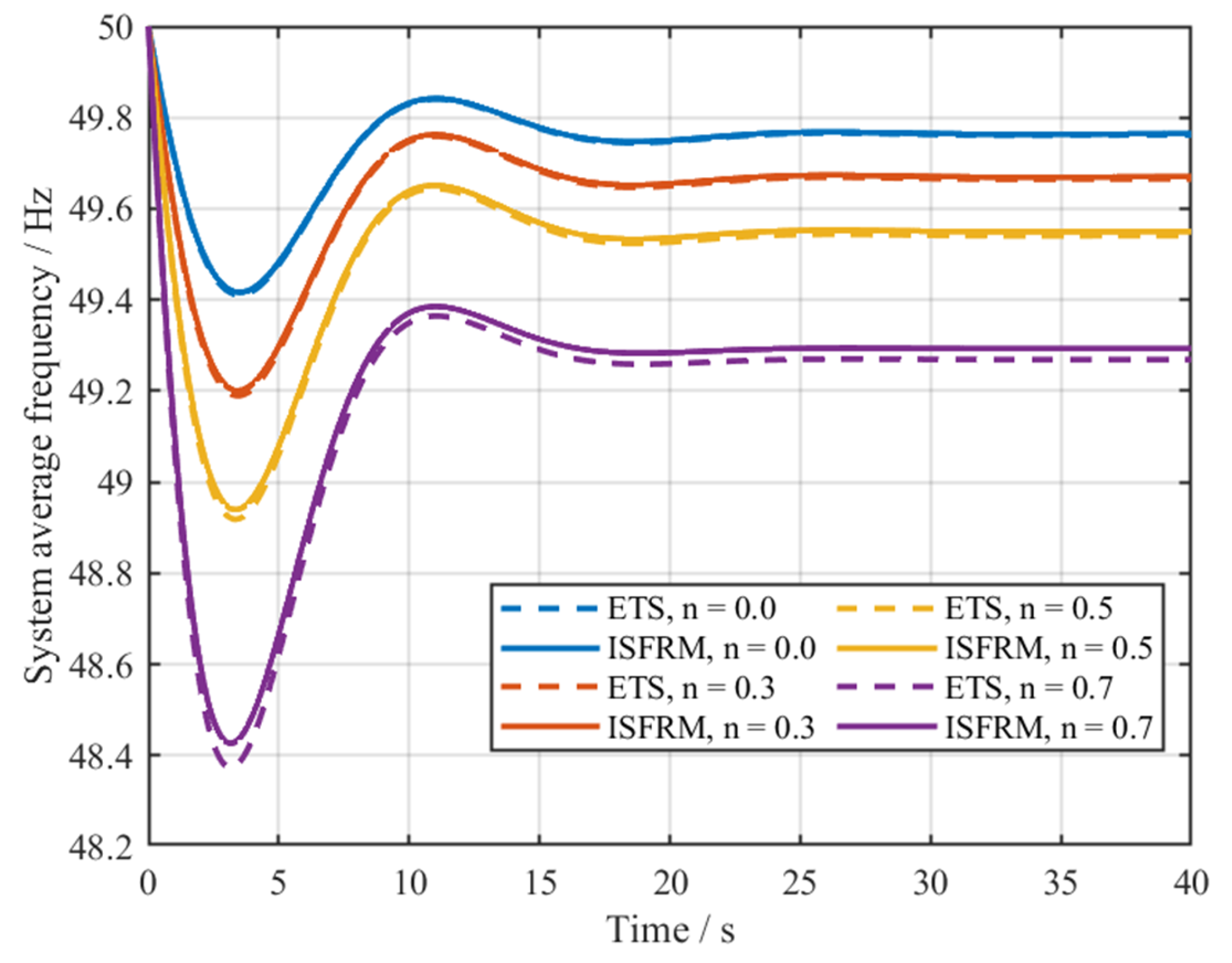
A MATLAB/Simulink (MATLAB Version R2023a) electromagnetic transient simulation (ETS) model, referred to as the ETS model in this paper, was established based on the modified nine-bus system wiring diagram, which can be found in the Supplementary Materials. For both the ETS model and the ISFRM, a proportional sudden increase of 10% in all load bus power was set at 0 s. Simulations were carried out under renewable energy penetration levels of 0%, 30%, 50%, and 70%, obtaining the transient simulation curves and frequency response model curves shown in Figure 3.

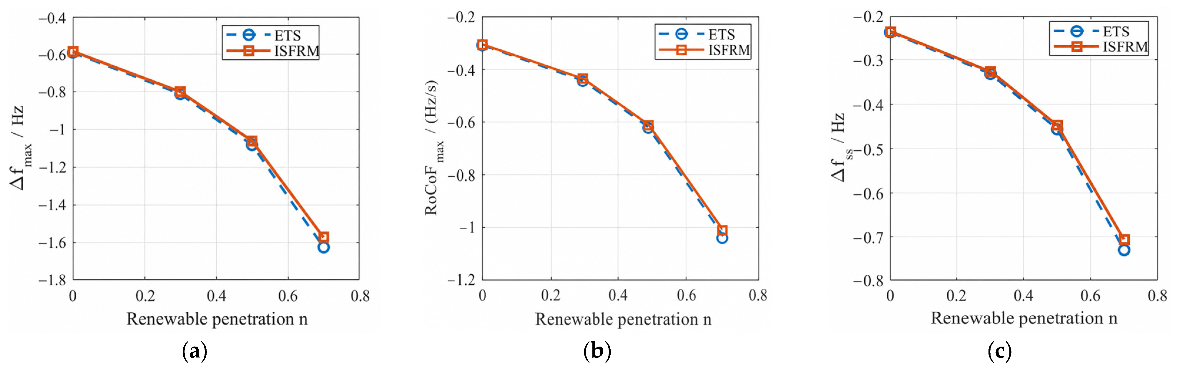
The variations of frequency characteristic indicators Δf_max, RoCoF_max, and Δf_ss are shown in Figure 4 and

Table 3. Quantitative validation of ISFRM against electromagnetic transient simulation.

Renewable Penetration n	Indicator	ETS Result	ISFRM Result	Absolute Error	Relative Error
0%	Δfmax (Hz)	−0.5893	−0.5835	0.0058	0.98%
0%	RoCoFmax (Hz/s)	−0.3121	−0.3090	0.0031	0.99%
0%	Δfss (Hz)	−0.2383	−0.2360	0.0023	0.97%
30%	Δfmax (Hz)	−0.8106	−0.7992	0.0114	1.41%
30%	RoCoFmax (Hz/s)	−0.4459	−0.4397	0.0062	1.39%
30%	Δfss (Hz)	−0.3350	−0.3303	0.0047	1.40%
50%	Δfmax (Hz)	−1.0816	−1.0603	0.0213	1.97%
50%	RoCoFmax (Hz/s)	−0.6245	−0.6122	0.0123	1.97%
50%	Δfss (Hz)	−0.4593	−0.4502	0.0091	1.98%

:

As shown in Table 3, the ISFRM closely matches the electromagnetic transient simulation results for the key frequency indicators. The relative errors of Δf_max, RoCoF_max, and Δf_ss are all below 5% under the tested renewable penetration levels, indicating that the ISFRM is sufficiently accurate for analyzing frequency security trends and supporting controllable load damping factor design.

In Figure 4, when renewable energy does not participate in frequency regulation, as the renewable energy penetration increases, the system frequency drop under the same unbalanced power disturbance deepens, and the system frequency characteristics deteriorate. Considering that the under-frequency load shedding frequency of Yunnan Power Grid is 49.2 Hz, for the three-machine nine-bus system in Table 1, when the renewable energy penetration reaches 30% or higher, a 10% system unbalanced power disturbance will cause a maximum frequency deviation exceeding −0.8 Hz, thereby triggering system under-frequency load shedding (UFLS) and reducing system power supply reliability.

3. Multi-Type Load Frequency Control Strategy for Power Systems

Frequent UFLS not only needlessly disconnects important loads, reduces power supply reliability and power quality, but also exacerbates fluctuations in grid operating parameters and is prone to trigger cascading negative effects, threatening the secure and stable operation of the power grid. To improve the frequency response characteristics of systems with high renewable energy penetration, it is necessary to exploit the frequency support potential of load-side resources. To this end, this section studies the frequency control implementation methods for Distribution Feeder Loads (DFLs), distributed constant power loads, and high-energy industrial loads, respectively, thereby realizing Multi-Type Load participation in system frequency regulation. In essence, load-side frequency control realizes the principle of “regulation instead of shedding” for loads, i.e., when a generation power deficit occurs in the system, the active power of loads is “regulated” through control means to prevent the frequency from dropping to the under-frequency load shedding trigger value, thereby avoiding large-scale blackouts caused by system “load shedding”.

3.1. Distribution Feeder Load Frequency Response Strategy

According to Equation (4), in the primary frequency regulation of the power system, the LDF can suppress frequency variations, and the larger D is, the more significant this effect is. In reference [20], the definition of the power system LDF is:

$$D={\displaystyle \frac{\Delta P_{\text{load}}}{\Delta f}}$$

(16)

where ΔP_load, Δf are the per-unit values of the load active power variation and frequency variation, respectively.

According to the definition of D, for the combination of several types of loads, the following should hold:

$$D_{\sum }={\displaystyle \frac{\Delta P_{\sum }^{*}}{\Delta f^{*}}}={\displaystyle {\displaystyle \sum _{i=1}^m}\frac{D_i{P}_i\Delta f^{*}}{\Delta f^{*}{P}_{\sum }}}={\displaystyle {\displaystyle \sum _{i=1}^m}{D}_i\frac{P_i}{P_{\sum }}}$$

(17)

That is, the LDF D_Σ of the power system is the weighted average of the LDFs of various types of loads in the system according to their capacity proportions. Therefore, the key to increasing the system LDF lies in enabling the active power of more types of loads to respond to grid frequency variations, reducing their own active power during low-frequency scenarios (i.e., when there is a power deficit in the system), thereby reducing the magnitude of the system unbalanced power and suppressing the system frequency drop.

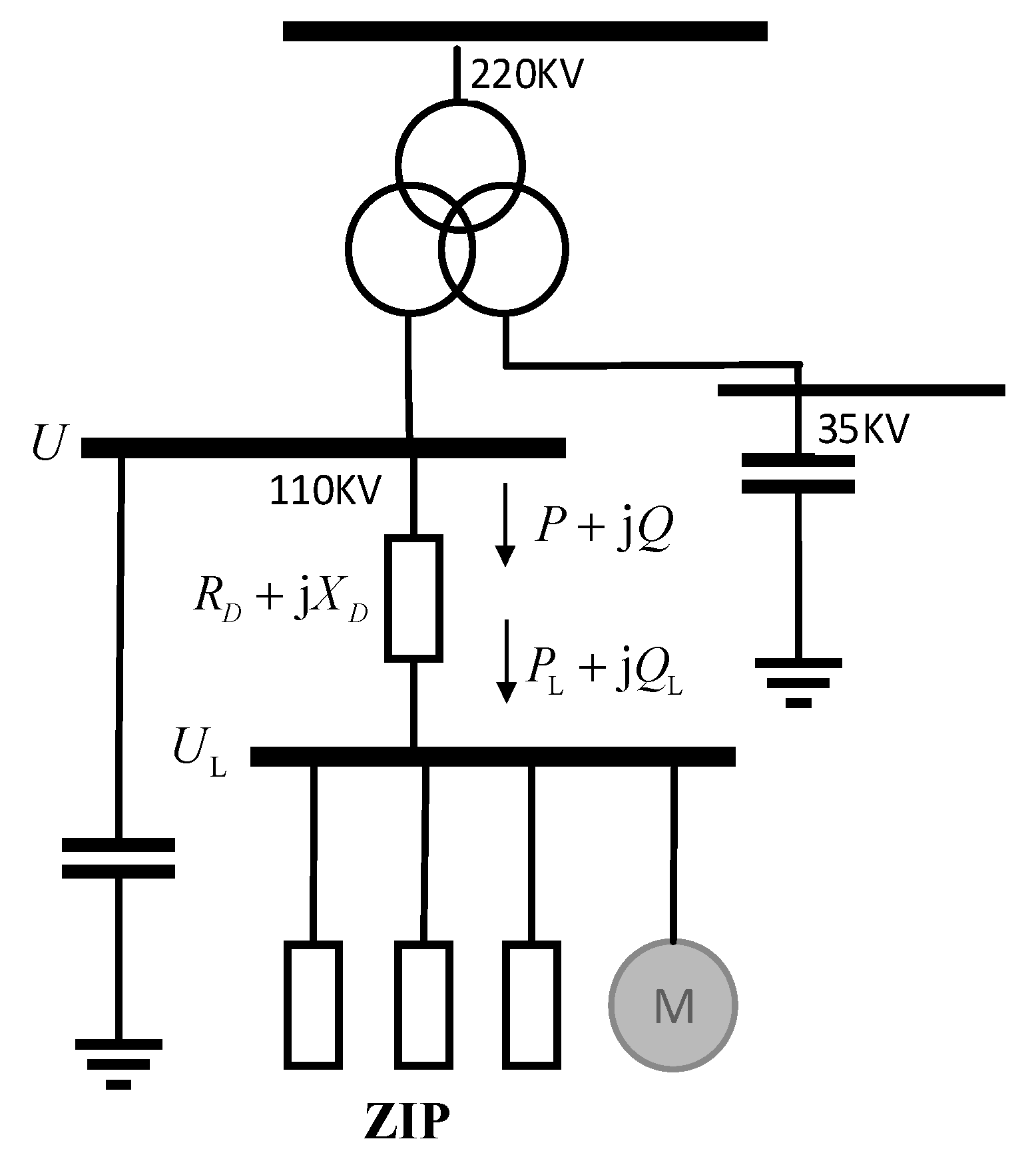
Figure 5 shows the power system synthesis load model (SLM). U_L denotes the equivalent feeder-side bus voltage of the synthesis load model.

In the power system Multi-Type Load model, only the induction motor loads (IMLs) are relatively sensitive to system frequency variations, while the active power of ZIP loads is insensitive to system frequency variations. Therefore:

$$P_{\mathrm{Z}IP}=P_{LN}\left[k_z{\left({\displaystyle \frac{V_L}{V_{N,L}}}\right)}^2+k_I\left({\displaystyle \frac{V_L}{V_{N,L}}}\right)+k_P\right]$$

(18)

where V_L denotes the feeder voltage, and V_N,L is its nominal rated value, P_LN is the rated power of the Multi-Type Load power system, P_ZIP is the sum of active power of constant impedance, constant current, and constant power loads in the system, k_z, k_i, and k_p are the proportions of ZIP loads in the Multi-Type Load P_LN, respectively, and the proportion of IMLs is denoted as k_m. From Equation (18), although constant impedance and constant current loads are insensitive to frequency variations, these types of loads are relatively sensitive to voltage; constant power loads are insensitive to both voltage and frequency. Reference [21] mentions that the active power of IMLs is sensitive to frequency variations and insensitive to voltage variations within the normal range. Therefore, this paper does not consider the impact of voltage on the active power of IMLs.

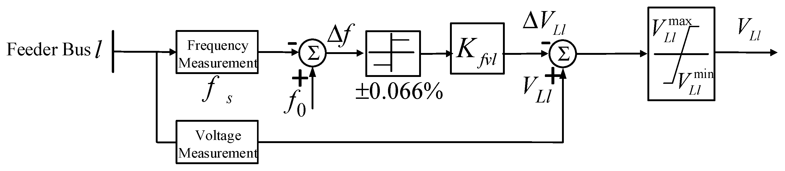
Since the power levels of constant impedance loads and constant current loads vary with changes in bus voltage, a frequency–voltage feedback control link can be constructed at the Multi-Type Load bus, using voltage regulation to indirectly change the load power, thereby realizing the active response of load power to system frequency deviations. In this context, these voltage-sensitive loads are treated as Distribution Feeder Loads (DFLs).

When a frequency deviation occurs in the system, the feedback gain K_fvl from the frequency deviation to the voltage regulation amount is introduced. The voltage change of the Multi-Type Load bus l can be described by Equation (19):

$$\Delta V_{Ll}=K_{fvl}\Delta f$$

(19)

where ΔV_Ll is the load voltage variation. Define K_Ll as:

$$K_{Ll}={\displaystyle \frac{\Delta P_{Ll}}{\Delta V_{Ll}}}$$

(20)

According to the definition of the LDF in Equation (16), the system LDF Dcl under controlled conditions is:

$$D_{cl}={\displaystyle \frac{\Delta P_{Ll}}{\Delta f}}={\displaystyle \frac{\Delta V_{Ll}}{\Delta f}}{\displaystyle \frac{\Delta P_{Ll}}{\Delta V_{Ll}}}=K_{fvl}{K}_{Ll}$$

(21)

Since in the Multi-Type Load model, regulating the bus voltage essentially adjusts the active power of the constant impedance and constant current loads, the following should hold:

$$D_{cl}\Delta f{P}_{lN}=D_Z\Delta f{P}_Z+D_I\Delta f{P}_I$$

(22)

Equation (22) indicates that the power of the regulated bus voltage equals the power variation of constant impedance and constant current loads. D_Z and D_I are the LDFs of the constant impedance load and constant current load after the introduction of control, respectively. Rearranging Equation (22) yields:

$$D_{cl}=k_Z{D}_Z+k_I{D}_I=k_{ZI}{D}_{ZI}$$

(23)

In Equation (23), k_ZI and D_ZI are the active power proportion and the LDF setting value of the voltage-sensitive loads after treating the ZI loads as a whole, respectively. According to Equation (20):

$$D_{ZI}={\displaystyle \frac{K_{fvl}{K}_{Ll}}{k_{ZI}}}$$

(24)

From Equation (17):

$$D_{\sum }={\displaystyle \sum _{i=1}^m{D}_i\frac{P_i}{P_{\sum }}}=k_M{D}_M+k_Z{D}_Z+k_I{D}_I+k_P{D}_P$$

(25)

Without control, D_Z, D_I, D_P are zero, so the natural LDF D₀ of the system is:

$$D_0=k_M{D}_M$$

(26)

After setting up the system frequency–voltage feedback control at the Multi-Type Load bus, D_Z and D_I are no longer zero. Therefore, the system LDF becomes:

$$D_{\sum }=k_M{D}_M+k_Z{D}_Z+k_I{D}_I=D_0+D_{cl}$$

(27)

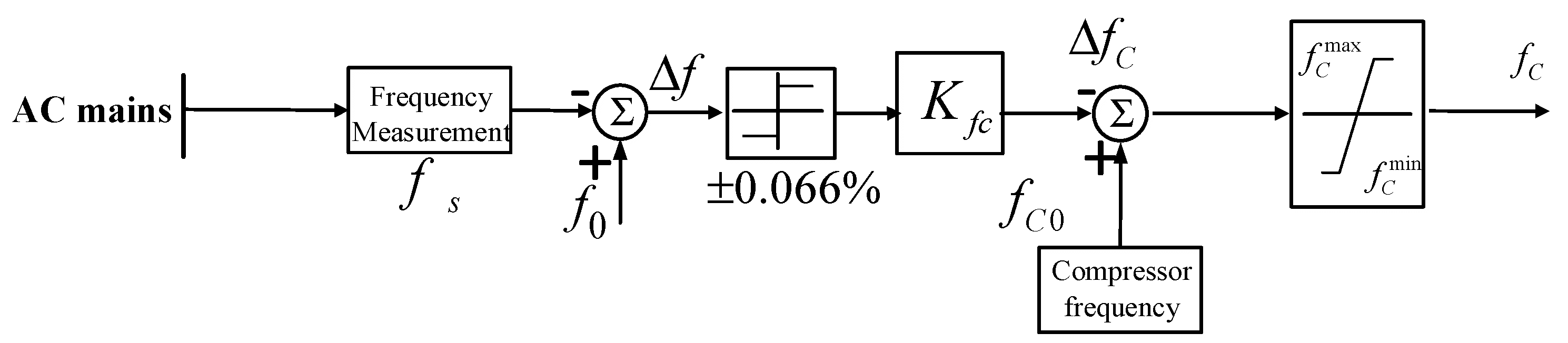
Through such a control strategy, the constant impedance loads and constant current loads in the DFL participate in grid frequency regulation, i.e., when the frequency decreases, the feeder voltage is reduced through the DFL frequency controller, reducing the active power of the voltage-sensitive loads, thereby increasing the system LDF D_Σ, as shown in Figure 6. The frequency deadband of ±0.033 Hz corresponds to approximately ±0.066% of the 50 Hz nominal frequency. This setting is used to prevent feeder voltage-sensitive loads from responding to small normal frequency fluctuations while allowing them to participate in primary frequency regulation during significant active power imbalance events.

3.2. Distributed Constant-Power Load Frequency Response Strategy

Section 3.1 proposed regulating the Multi-Type Load feeder voltage to achieve power regulation of voltage-sensitive loads in the DFL, which is equivalent to changing the LDFs of constant impedance and constant current loads from 0 to a controllable value. However, constant power loads are insensitive to both frequency and voltage, so a more refined load model is usually needed for power control. Typical constant-power distributed loads in the Multi-Type Loads include electric vehicle charging stations, variable frequency motor loads, switching power supply loads, etc. This section takes the inverter air conditioner (IAC) load as a representative to study the frequency control strategy for distributed constant-power loads.

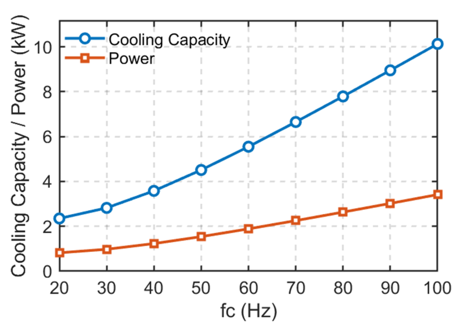
As shown in Figure 7, the cooling capacity Q_IAC and electrical power P_IAC of IAC are positively correlated with the compressor frequency f_c.

Q_IAC and P_IAC can be calculated by Equations (28) and (29) [22]:

$$Q_{IAC}={\displaystyle \frac{k_Q}{T_{IAC}s+1}}{f}_c+{\mu }_Q$$

(28)

$$P_{IAC}={\displaystyle \frac{k_P}{T_{IAC}s+1}}{f}_c+{\mu }_P$$

(29)

where Q_IAC and P_IAC represent the rated cooling capacity and electrical power, both in kW; f_c is the compressor frequency, in Hz; T_IAC represents the compressor inertia time constant, taken as 0.02; k_Q and μ_Q represent the constant coefficients of the IAC cooling capacity, with values of 0.12 kW/Hz and −0.05 kW, respectively; k_P and μ_P represent the constant coefficients of IAC operating power.

From Equation (29), for the IAC load, continuous power regulation can be achieved by adjusting the compressor frequency. To enable the IAC load to participate in system frequency regulation, a feedback control link from grid frequency deviation to compressor frequency is added to the original temperature-control operation of IAC, as shown in Figure 8.

The controller first measures the bus frequency f_s in real time and compares it with the rated frequency f₀ to obtain the system frequency deviation:

$$\Delta f=f_s-f_0$$

(30)

Through the regulation coefficient K_fc, the grid frequency deviation signal is converted into the compressor frequency correction amount Δf_c, i.e.,

$$\Delta f_c=K_{fvl}\Delta f$$

(31)

This correction amount is then superimposed with the compressor base frequency f_c0 generated by the original temperature-control logic to obtain the new compressor frequency command:

$$f_c^{*}=f_{c0}+\Delta f_c$$

(32)

The active power of IAC satisfies a first-order inertia relationship with the compressor frequency. Therefore, after adding the control, the IAC active power can be expressed as:

$$P_{IAC}={\displaystyle \frac{k_P}{T_{IAC}s+1}}{f}_c^{\ast }+{\mu }_P$$

(33)

The implementation process of frequency control can be summarized as: when the system frequency drops, the controller detects a negative frequency deviation and appropriately reduces the compressor frequency, thereby reducing the IAC active power; when the system frequency recovers, the additional correction amount gradually decreases, and the IAC operating state returns to the original temperature-control level.

The change in IAC power caused by the compressor frequency variation is:

$$\Delta P_{IAC}(s)={\displaystyle \frac{k_P}{T_{IAC}s+1}}\Delta f_c(s)$$

(34)

Substituting $\Delta f_c=K_{fvl}\Delta f$ yields:

$$\Delta P_{IAC}(s)={\displaystyle \frac{k_p{K}_{f\mathrm{c}}}{T_{IAC}s+1}}\Delta f(s)$$

(35)

Therefore, the controlled LDF transfer function of a single IAC is:

$$D_{IAC}(s)={\displaystyle \frac{\Delta P_{IAC}(s)}{\Delta f(s)}}={\displaystyle \frac{k_p{K}_{fc}}{T_{IAC}s+1}}$$

(36)

Neglecting the inertia time constant of the IAC unit, under quasi-steady-state conditions, the controlled LDF of a single IAC can be expressed as:

$$D_{IAC}=\underset{s\to 0}{\lim }{D}_{IAC}(s)=k_P{K}_{fc}$$

(37)

3.3. Energy-Intensive Industrial Load Frequency Response Strategy

Without additional control means, electrothermal energy-intensive industrial loads can also be regarded as constant-power loads. Yunnan Province possesses a large number of energy-intensive electrolytic aluminum (EA) loads, which inherently have considerable capacity to participate in grid frequency regulation. Reference [23] mentions that EA, as a thermal energy storage load, can maintain heat preservation and continuous operation for 4 h under a 25% reduction in active power.

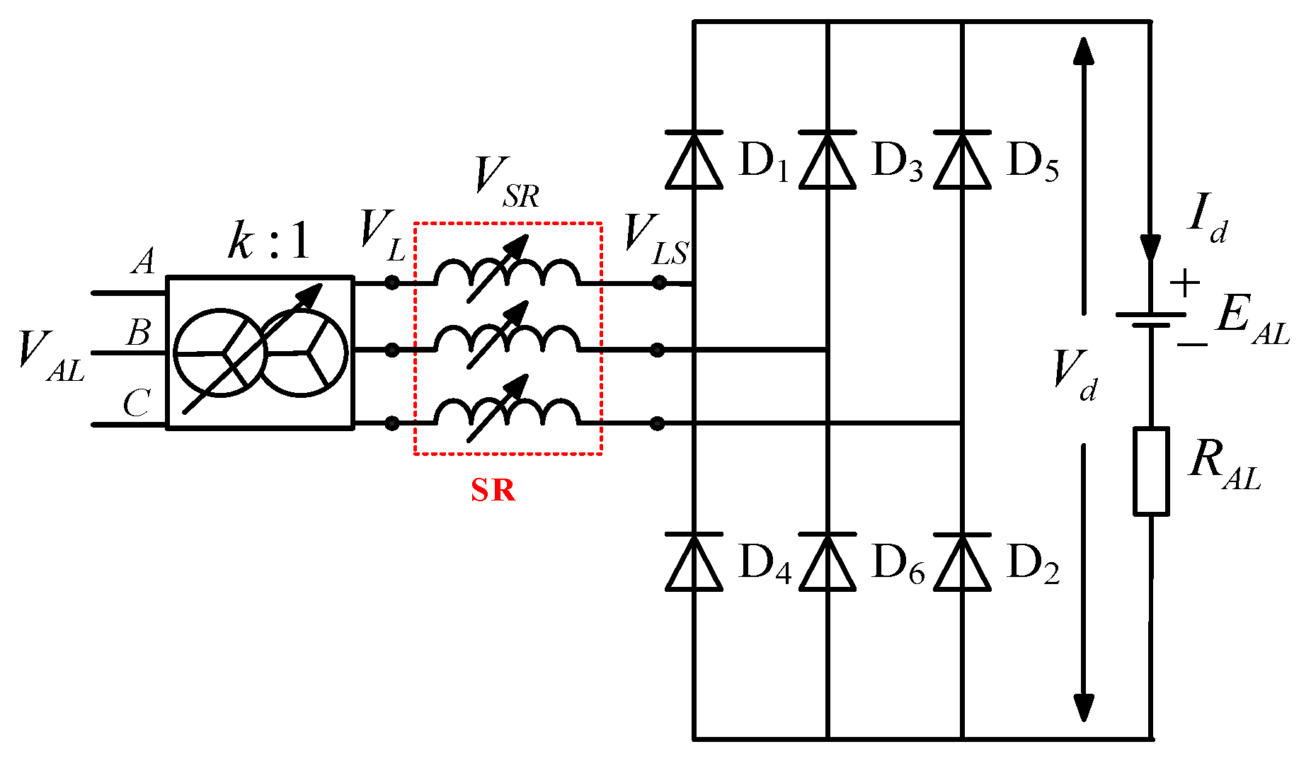
The basic process of EA smelting involves continuously supplying hundreds of kiloamperes of direct current to the electrolytic cell, causing alumina to undergo an electrolytic reaction and produce crude aluminum in a cryolite–alumina molten salt system at a high temperature of approximately 950–970 °C. In engineering applications, the alternating current usually needs to be converted to direct current through an 84-pulse rectification system before being delivered to the electrolytic cell. Figure 9 shows the practical equivalent circuit of EA rectification. In Figure 9, V_AL is the bus voltage of the aluminum plant, k is the rectifier transformer ratio, V_SR is the voltage drop of the saturable reactor, V_LS is the AC side voltage of the EA rectifier bridge, D1–D6 are rectifier diodes, and E_AL and R_AL are the equivalent resistance and equivalent back electromotive force of the electrolytic cell on the DC side of the EA, respectively [24].

According to Figure 9, the DC voltage of the electrolytic cell can be expressed as:

$$V_d={\displaystyle \frac{3\sqrt{2}}{\pi }}\left({\displaystyle \frac{V_{AL}}{k}}-V_{SR}\right)$$

(38)

The active power P_AL of the EA load can be expressed as:

$$P_{AL}=g\left(V_{AL},V_{SR}\right)={\displaystyle \frac{\left(V_d-E_{AL}\right)}{R_{AL}}}{V}_d$$

(39)

From Equations (38) and (39), the active power of EA is mainly determined by the bus voltage V_AL on the high-voltage side of the aluminum plant’s main transformer, the transformer ratio k, and the saturable reactor voltage drop V_SR.

According to Reference [24], adjusting the control current of the saturated reactor can regulate its voltage drop V_SR, thereby realizing millisecond-level fast and continuous control of electrolytic aluminum load power. When changing the active power of the EA load by adjusting the saturable reactor voltage drop V_SR, according to Equations (38) and (39), the target value for the adjustment of the saturable reactor voltage drop V_SR should be:

$$V_{SR}={\displaystyle \frac{V_{AL}}{k}}-{\displaystyle \frac{\sqrt{2}\pi }{6}}{V}_d={\displaystyle \frac{V_{Pb}}{k}}-{\displaystyle \frac{\sqrt{2}\pi }{12}}\left(E_{AL}+\sqrt{E_{AL}^2-4R_{AL}{P}_{ALN}\left(1+\Delta P_{AL}\right)}\right)=g(\Delta P_{AL})$$

(40)

In Equation (40), ΔP_AL is the per-unit value of the active power regulation amount of EA participating in frequency control, calculated by Equation (41):

$$\Delta P_{AL}=-D_{AL}\Delta f$$

(41)

where D_AL is the setting value of the EA LDF.

Figure 10 shows the EA load frequency controller. Without additional frequency control, the LDF of the EA load is zero, i.e., the EA active power does not vary with the grid frequency. After adding the controller, the EA load will respond to grid frequency variations according to the D_AL setting value, increasing the saturable reactor voltage drop V_SR and reducing its own active power when the frequency decreases, thus participating in the primary frequency regulation of the power grid.

4. Case Study Analysis

4.1. Case Study Grid Topology

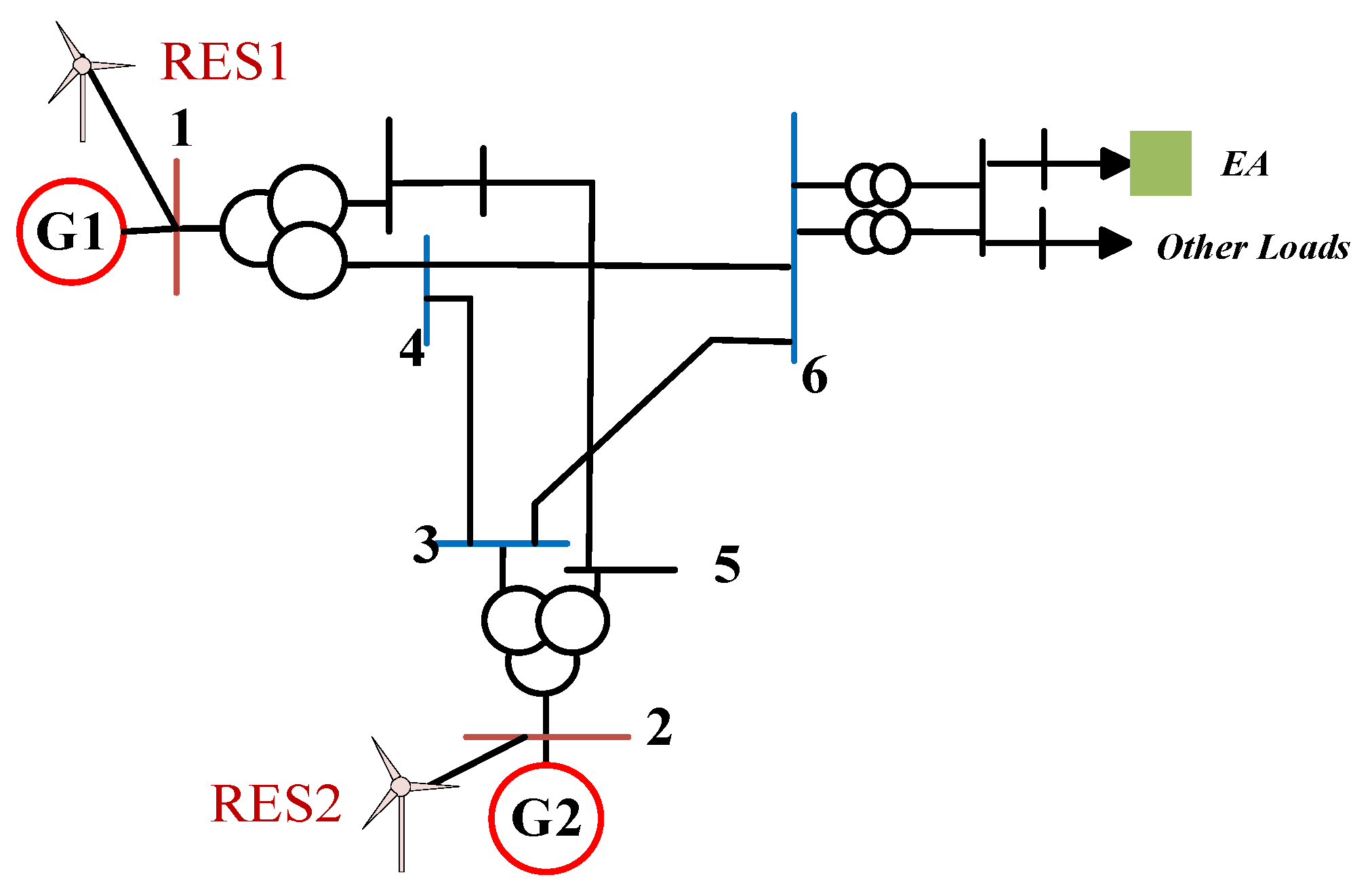
Figure 11 shows the simplified topology of an actual power grid in a certain area of Yunnan. This regional grid is a receiving-end grid, with the two incoming lines equated to equivalent generating units G1 and G2, respectively. Similar to the modified IEEE nine-bus validation system, renewable penetration n is modeled by proportionally replacing the equivalent synchronous generation capacity and active power output at the corresponding generation-side connection points. This chapter uses this topology as a case study to verify the improvement effects of load-side frequency control on the grid frequency response characteristics and renewable energy accommodation capacity.

The grid-connected parameters of the generation-side equipment in the case study grid are shown in

Table 4. Equivalent grid-connected parameters of thermal power units and renewable energy equipment in the case study grid.

Grid Node	Grid-Connected Capacity Sum of Thermal and Renewable Energy Si/MVA	Active Power Output Sum of Thermal and Renewable Energy Pi/MW	Inertia Time Constant of Thermal Power Unit HGi/s	Regulation Coefficient of Thermal Power Unit RGi/s	System Load Damping Factor D
1	1440	1024.5	4	0.04	0.33
2	6000	4268.8	4	0.04

, and the power and adjustable capacity of various types of loads are shown in

Table 5. Load types and adjustable power settings of the case study grid topology.

Load type	Original Active Load/MW	Active Power Proportion	Maximum Power Down-Regulation Ratio	Maximum Regulated Downward Power/MW	Natural/Controlled Load Damping Factor
Electrolytic Aluminum Load	3500	0.661	20%	700	DAL
Feeder Voltage-Sensitive Load	500	0.094	10%	50	DZI
Feeder Distributed Constant Power Load	323.4	0.061	20%	64.68	DP
Feeder Induction Motor Load	970.6	0.183	20%	194.12	1.8

. Among them, EA loads, DFLs, and distributed constant power loads are controlled loads. IMLs do not have additional control means applied, and their active power relies on their own natural LDF to respond to grid frequency variations. The reference value of the IML LDF in Table 5 is obtained from actual measurements.

The load power regulation amount after load frequency control is:

$$\Delta P_{Li}=\left\{\begin{array}{l}0,f\ge f_{DB}\\ P_{LNi}{D}_{ci}\Delta f^{*},f_l<f\le f_{DB}\\ \Delta P_{Li-\max },f<f_l\end{array}\right.$$

(42)

where D_ci is the setting value of the controlled LDF for each type of load, f_DB is the frequency regulation dead band of the controlled LDF, and f_l is the frequency corresponding to the load reaching its maximum regulation amount.

According to Equation (17), the system LDF is:

$$D_{\sum }=0.661D_{AL}+0.094D_{ZI}+0.061D_P+0.183*1.8$$

(43)

Let D_AL = D_P = 2D_Z = Ds to ensure that various types of loads simultaneously reach their upper regulation limits under large disturbances. Then:

$$D_{\sum }=0.77D_s+0.33$$

(44)

Under this condition, this situation is equivalent to adding a controlled LDF Ds to the aggregated load accounting for 0.77 of the system. The maximum downward regulation power of the aggregated load is 814.8 MW.

4.2. Analysis of the Improvement Effect of Multi-Type Load-Based Frequency Regulation Strategy on System Frequency Response Characteristics

This section verifies the improvement effect of the load frequency control strategy on system frequency response characteristics by building an ETS model of the case study grid in MATLAB/Simulink (MATLAB Version R2023a), which can be found in the Supplementary Materials.

4.2.1. Analysis of Controlled Load Power Response with Frequency Variation

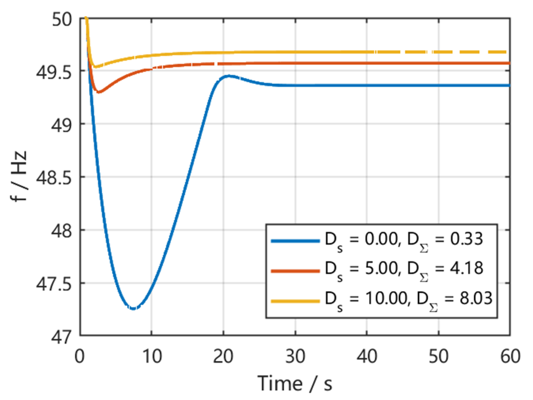
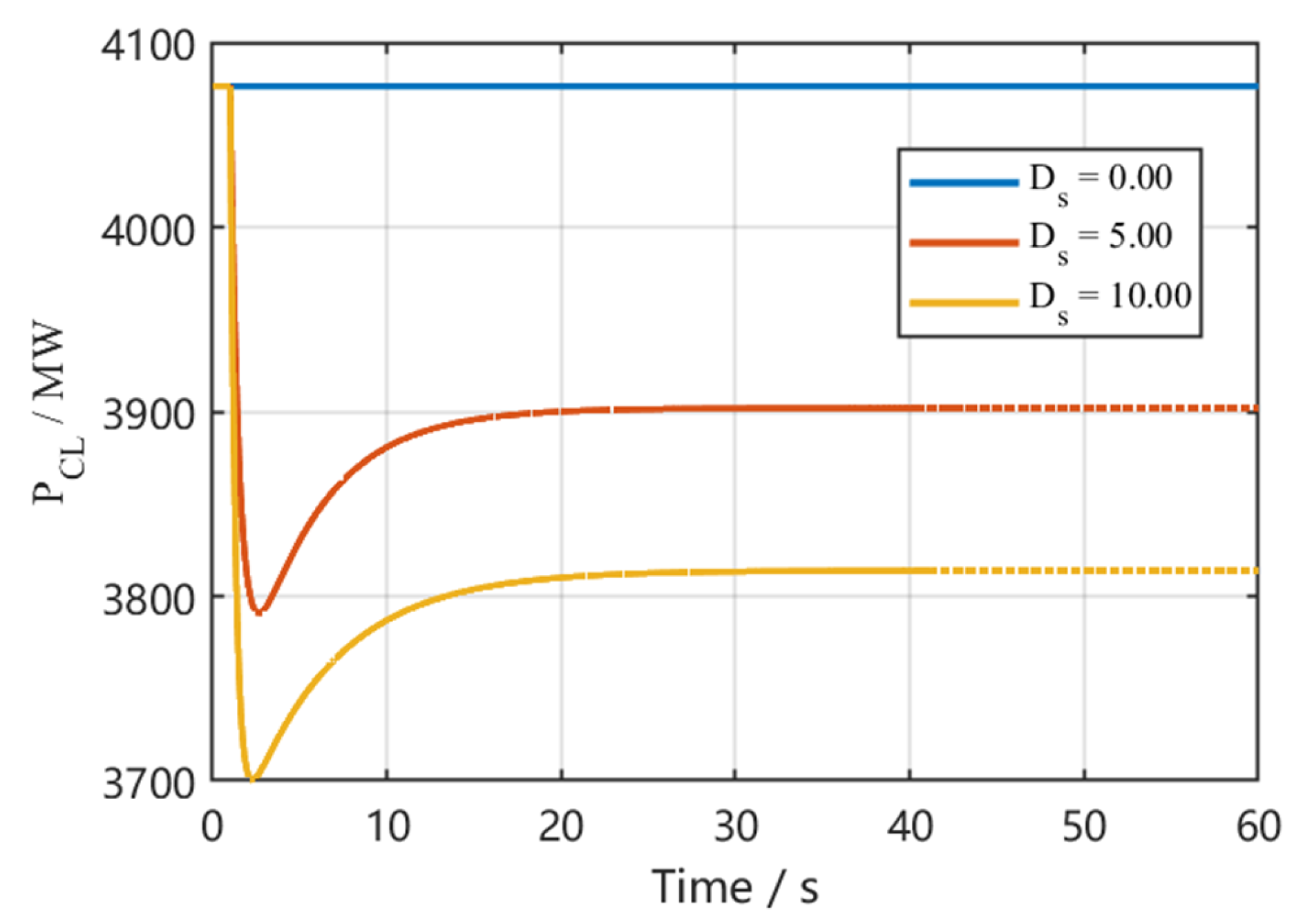
Setting the renewable energy penetration at 70%, simulations are carried out under a −0.1 p.u. active power disturbance. The system frequency response curves corresponding to different Ds setting values are shown in Figure 12, and the corresponding controlled load active power curves are shown in Figure 13.

Figure 13 shows the variation of controlled load power with frequency after the disturbance occurs. When D_s = 0, the controlled loads are not engaged in frequency regulation, and their active power remains unchanged. After increasing D_s, in the initial stage of the disturbance, the frequency regulation support power of the controlled loads rises rapidly and reaches a peak, indicating that the loads can respond quickly to the frequency drop. Subsequently, as the system frequency gradually recovers, the support power falls back from the peak and finally stabilizes at a certain level, corresponding to the actual active power of the controlled loads recovering from the nadir to a new stable value. In Figure 12, as the setting value of the controlled LDF D_s increases, the degree of system frequency drop under unbalanced power disturbance is significantly alleviated, indicating that the application of the load frequency control strategy proposed in this paper has a significant improvement effect on system frequency response characteristics.

4.2.2. Analysis of System Frequency Response Characteristics Under Different n and D_s Simulation Scenarios

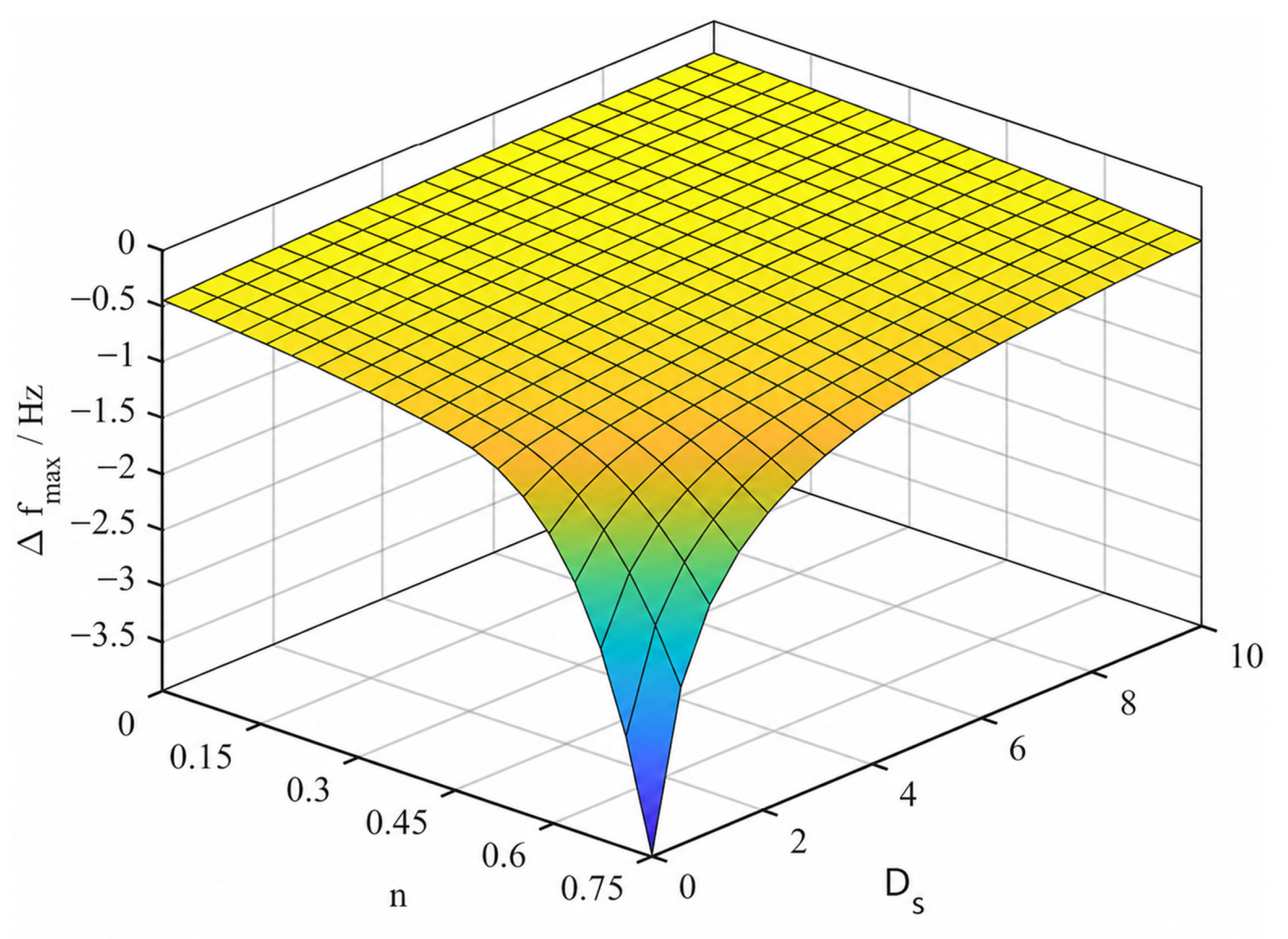
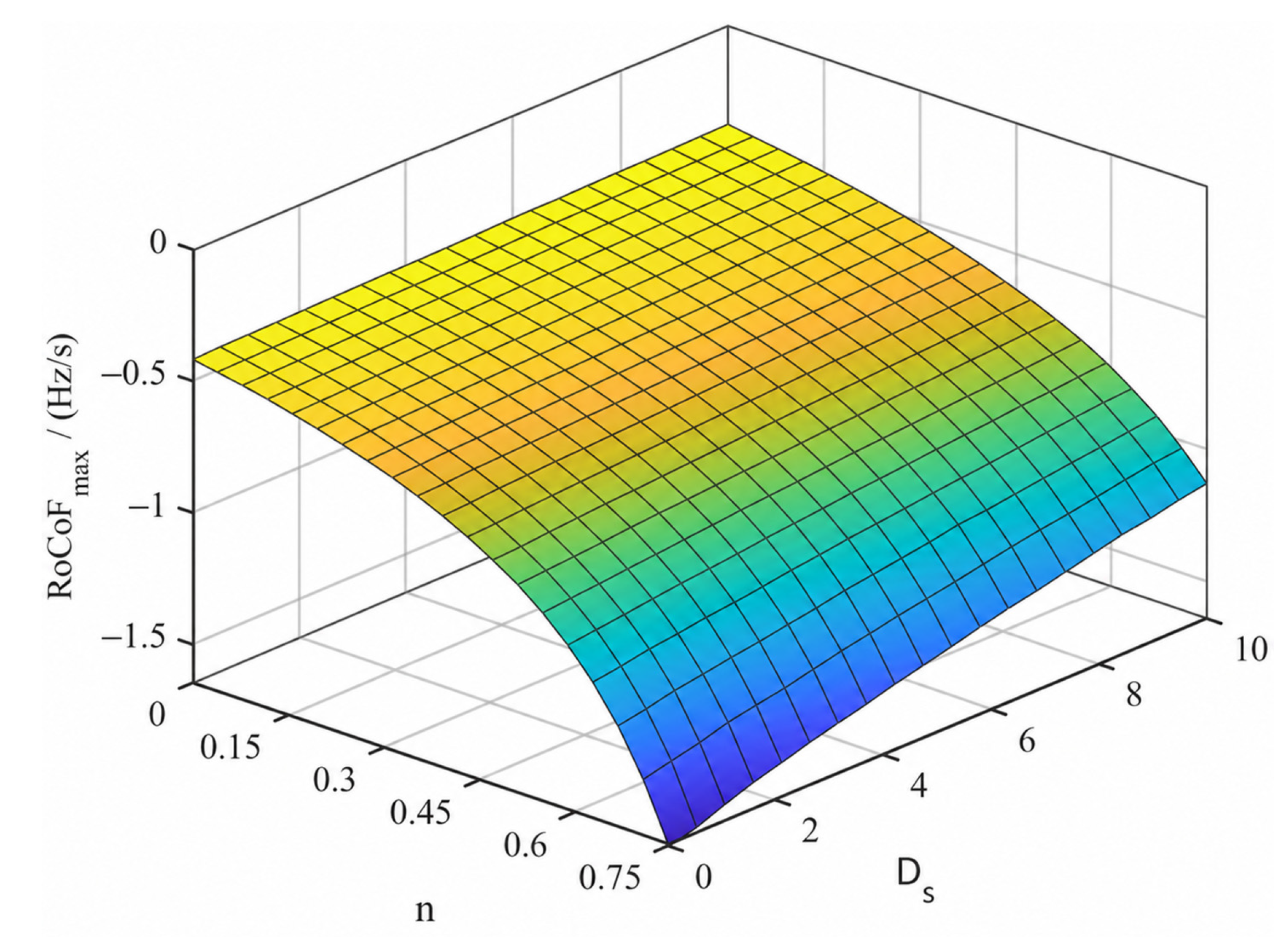
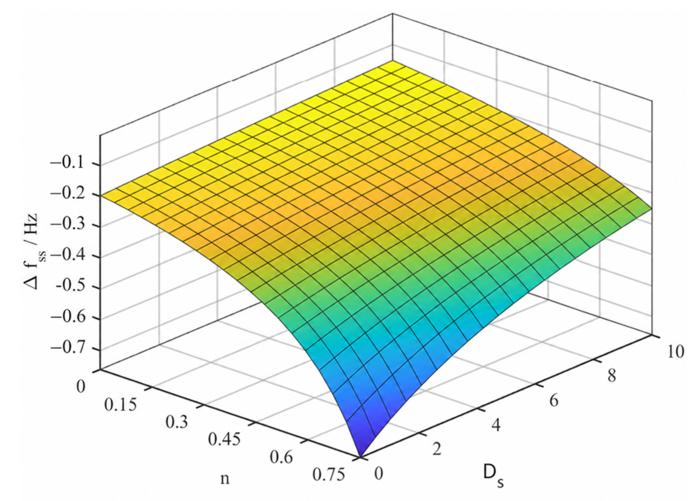
Furthermore, taking the system unbalanced power of −0.1 p.u. as the assessment index, the key parameters of system frequency response characteristics, RoCoF_max, Δf_max, and Δf_ss, are obtained under different simulation scenarios of system renewable energy penetration n and different controlled LDF Ds, as shown in Figure 14, Figure 15 and Figure 16.

In Figure 14, Figure 15 and Figure 16, under −0.1 p.u. disturbance power, |RoCoF_max|, |Δf_max|, |Δf_ss| increase with the rise of renewable energy penetration in the system, indicating that a higher renewable energy penetration worsens the system frequency response characteristics. Conversely, |RoCoF_max|, |Δf_max|, and |Δf_ss| decrease significantly with the increase of the controlled LDF Ds.

4.2.3. Analysis of the Improvement Effect of Load Frequency Control Strategy on Renewable Energy Accommodation Capacity

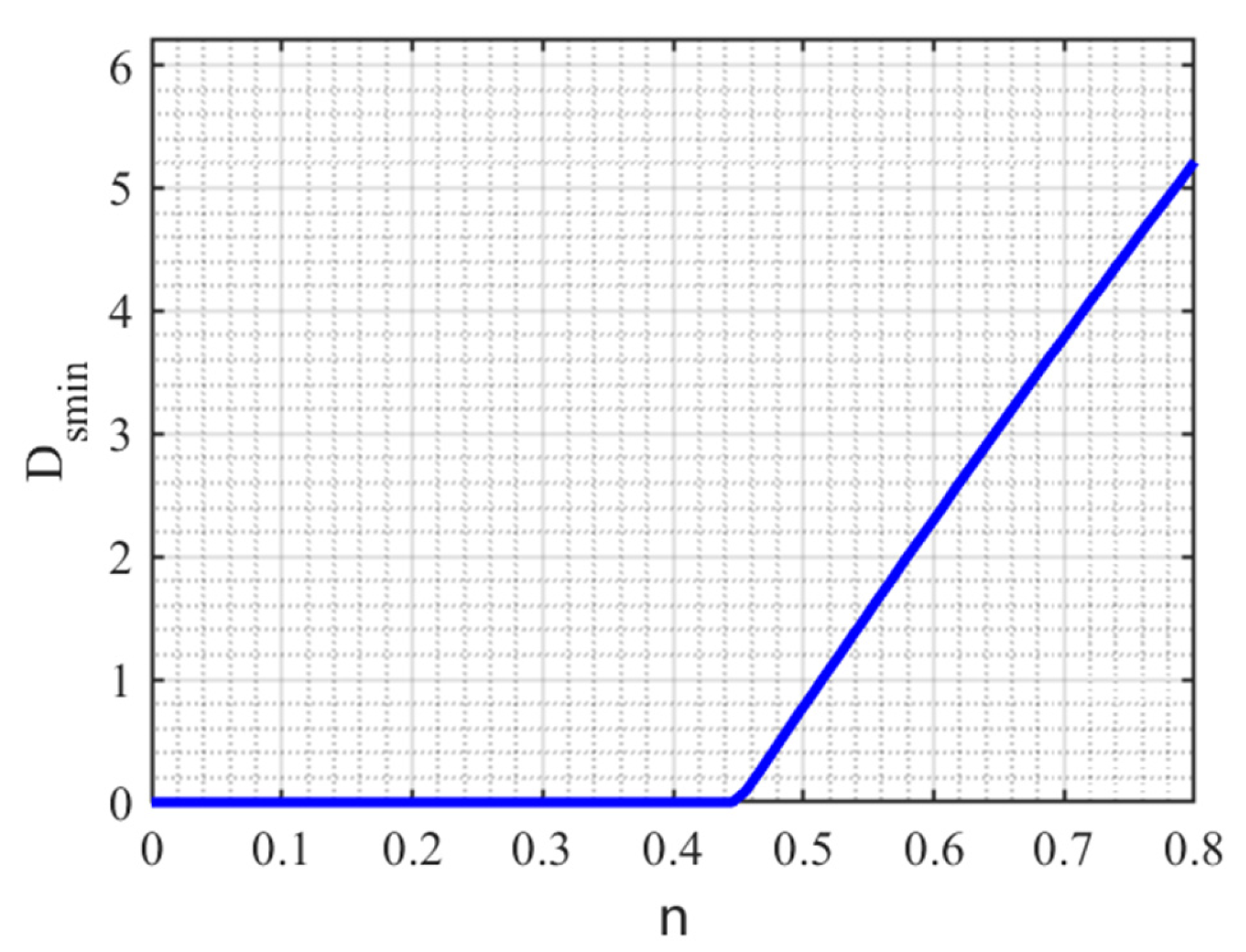
Since the UFLS threshold of China’s Yunnan Power Grid is 49.2 Hz, the corresponding allowable transient maximum frequency deviation Δf_{max_limit} is –0.8 Hz. To accurately avoid triggering system UFLS, it is necessary to evaluate the minimum required Ds setting value, i.e., D_smin, under different simulation scenarios. The intersection curve of the Δf_max surface and the Δf_max = −0.8 Hz plane in Figure 14 yields the D_smin–n curve shown in Figure 17. The region above the curve corresponds to scenarios where UFLS is not triggered, while below the curve the system UFLS will be triggered.

According to Figure 17, without the load frequency control strategy applied, under a −0.1 p.u. disturbance power, when the renewable energy penetration exceeds 44%, system UFLS will be triggered. Therefore, under the UFLS frequency constraint, the renewable energy accommodation capacity of the studied grid is approximately 44%. However, when D_s = 5, the system can still avoid triggering UFLS under 70% renewable energy penetration and –0.1 p.u. disturbance power, indicating that the proposed load frequency control strategy can significantly improve the renewable energy accommodation capacity of the system.

4.3. Economic Analysis of Controlled Loads Participating in Frequency Regulation

Existing studies often focus on renewable energy sources such as wind and solar participating in frequency regulation to prevent the deterioration of system frequency response characteristics caused by increasing renewable energy penetration. However, when renewable energy units deviate from their maximum power output operation, curtailment of wind and solar power inevitably occurs, reducing the revenue from the corresponding electricity sales. Taking the Yunnan Province renewable energy on-grid price λ = 0.3358 yuan/kWh as the curtailment cost for renewable energy participating in frequency regulation, the proposed load frequency control strategy exhibits a significant economic advantage in comparison.

4.3.1. Economic Analysis of DFL Frequency Regulation

The cost of DFL frequency regulation mainly consists of the equipment cost of the controlled LDF controller (the core device being a voltage regulating device such as SVG). The controller cost F comprises investment cost and maintenance cost, as expressed in Equation (45):

$$F=C_{inv}+C_m$$

(45)

where C_inv is the annualized investment cost, and C_m is the annual maintenance cost. The expression for C_inv is:

$$C_{inv}=C(r,l)(1-{\lambda }_{st})C_V{S}_V$$

(46)

$$C(r,l)={\displaystyle \frac{r{(1+r)}^l}{{(1+r)}^l-1}}$$

(47)

where r is the discount rate of the controller, l is the life cycle of the controller, λ_st is the residual value coefficient of the controller, C_V is the investment cost per-unit capacity, and S_V is the capacity of the controller.

The expression for C_m is:

$$C_m=S_V*b_V$$

(48)

where b_V is the maintenance cost coefficient.

The unit investment cost of the DFL controlled LDF controller is approximately 150 yuan/kvar, the maintenance cost coefficient is 0.02 yuan/kvar, the life cycle is 10 years, the residual value coefficient is 0.5, and the discount rate is 0.1 [21].

The controller cost is converted per unit of frequency regulation capacity using the following formula:

$$(C(r,l)(1-{\lambda }_{st})C_V{S}_V+S_V{b}_V)/\Delta P_L$$

(49)

According to [21], a LDF controller with a capacity of 25% of the transformer capacity can achieve a system active power regulation of 6.2%. Thus, the annual frequency regulation cost of the DFL is 48.7 yuan/(kW·year), which is far lower than the curtailment cost of 2941.61 yuan/(kW·year) (calculated based on the Yunnan renewable energy on-grid price of 0.3358 yuan/kWh).

4.3.2. Economic Analysis of Distributed Load Frequency Regulation

For small-capacity distributed constant power loads such as inverter air conditioners and switching power supply loads, large-capacity power electronic main equipment is usually not required. The cost of power regulation for such loads mainly comes from a certain degree of sacrifice in user comfort, such as air conditioning cooling effect, lighting intensity, battery charging speed, etc.

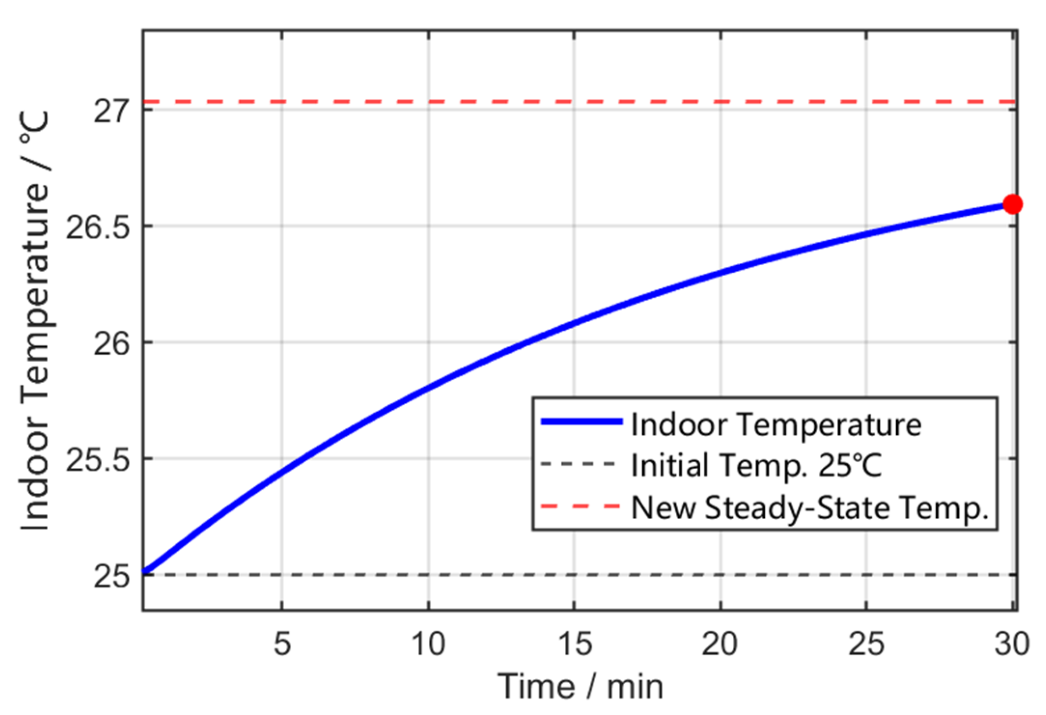
Taking IAC loads as an example, in peak-shaving services of demand response, load aggregators usually need to consider user thermal comfort and provide compensation to users [25]. However, IACs operate under indoor thermal inertia conditions. The relationship between indoor temperature and IAC cooling capacity is given by Equation (50):

$$C_{\mathrm{m}}{R}_{\mathrm{m}}{C}_{\mathrm{a}}{\displaystyle \frac{{\mathrm{d}}^2{\theta }^{\text{in}}}{\mathrm{d}{t}^2}}+\left(C_{\mathrm{m}}+C_{\mathrm{a}}+{\displaystyle \frac{C_{\mathrm{m}}{R}_{\mathrm{m}}}{R_{\mathrm{e}}}}\right){\displaystyle \frac{\mathrm{d}{\theta }^{\mathrm{in}}}{\mathrm{d}t}}=-Q_{IAC}+{\displaystyle \frac{T_{\text{out}}-T_{in}}{R_{\mathrm{e}}}}$$

(50)

where Q_IAC represents the cooling capacity of the IAC; C_a and C_m are the specific heat capacities of air and solid, respectively; R_e is the thermal resistance between indoor and outdoor; R_m is the solid thermal resistance; θ_in and θ_out are the indoor and outdoor temperatures, respectively.

The simulation scenario is set as follows: the initial indoor temperature is 25 °C, the outdoor temperature is 35 °C, and R_e =0.0013 K/W. The cooling capacity and power of the IAC satisfy Equations (28) and (29). Before t = 0, it is assumed that the indoor and outdoor environment is in a heat exchange equilibrium state, i.e.,

$$-Q_{IAC}+{\displaystyle \frac{T_{\mathrm{out}}-T_{in}}{R_{\mathrm{e}}}}=0$$

(51)

At t = 0, the IAC cooling power is reduced by 20%. The changes in compressor frequency f_c, cooling power P_IAC, and cooling capacity Q_IAC before and after the reduction are shown in

Table 6. Parameter changes before and after 20% reduction in IAC power.

Compressor Frequency/Hz		Cooling Power/kW		Cooling Capacity/kW		Indoor Temperature/°C
Before Change	After Change	Initial Value	After Reduction	Initial Value	After Reduction	Original Steady-State Temperature	New Steady-State Temperature
64.5192	51.5154	2.6008	2.0806	7.6923	6.1318	25 °C	27.0286 °C

:

Figure 18 shows the variation of indoor temperature over time. Under this working condition, a 1 °C change corresponds to a time scale on the order of tens of minutes, which means that short-time-scale regulation during primary frequency control has a minimal impact on the comfort of IAC users. Therefore, IAC loads have good frequency regulation economy, and this paper does not consider frequency regulation compensation costs from the perspective of user comfort.

4.3.3. Economic Analysis of Energy-Intensive Industrial Load Frequency Regulation

Unlike distributed constant power loads, energy-intensive industrial loads bear production tasks themselves, and the frequency regulation cost for participating in primary frequency control mainly comes from production losses caused by electricity consumption reduction.

Taking EA loads as an example, EA loads have a huge thermal inertia. Moderately reducing smelting power for a short time generally does not cause significant fluctuations in the temperature of the electrolytic cell. Therefore, appropriate power regulation does not affect the production continuity of the aluminum plant, but the power reduction during the electrolysis process means that the EA production in that period will decrease accordingly. Since EA production is approximately proportional to electricity consumption, the economic cost of its participation in frequency regulation can usually be evaluated by the reduction in EA electricity consumption, i.e., the integral of the active power regulation amount over time.

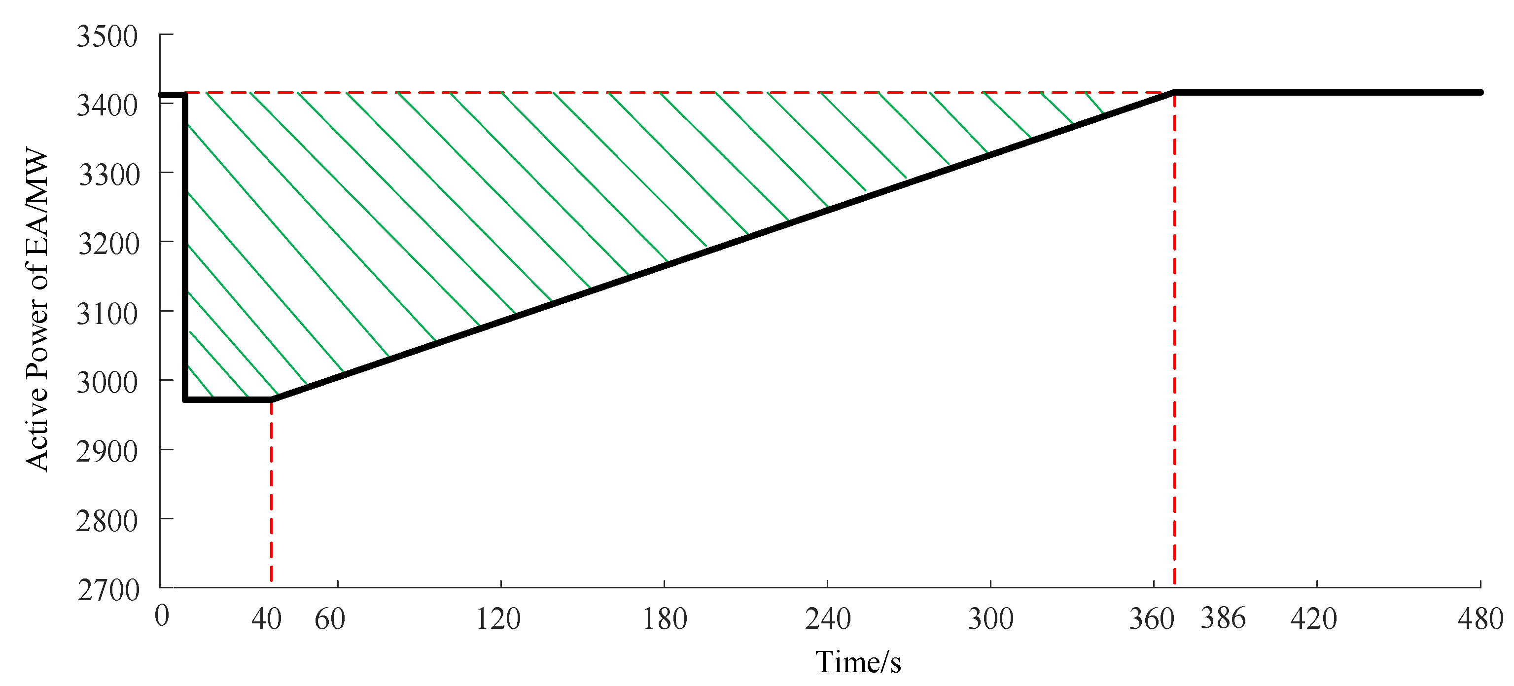
Taking the process shown in Figure 19 as an example, when a large power imbalance occurs in the system, after the EA controlled LDF control is engaged, corresponding to the rapid increase in grid frequency deviation at the initial moment of the disturbance, the EA load first rapidly reduces power to provide frequency support. Subsequently, after the secondary frequency regulation reserve is put into operation, the AGC units detect the area tie-line power deviation and continuously increase their output. As the AGC regulation effect gradually increases, the system frequency deviation continuously converges, and the EA load gradually restores to its original operating level [19].

The area of the shaded region in Figure 19 reflects the reduced electricity consumption of the EA load during the entire frequency regulation process. Multiplying this portion of electricity loss by the unit electricity profit of the aluminum plant allows estimation of the revenue loss caused by its participation in frequency control. Reference [24] mentions that the unit electricity economic profit of an EA plant is about 0.176 yuan/kWh, which is only 52.4% of the Yunnan renewable energy on-grid price of 0.3358 yuan/kWh. Therefore, the cost of EA participating in primary frequency regulation is also far lower than that of renewable energy units.

5. Conclusions

To address the deterioration of frequency response characteristics caused by high renewable energy penetration in new-type power systems, this paper proposes a Multi-Type Load frequency control strategy for high-renewable power systems. System modeling, frequency response analysis, and electromagnetic transient simulations are conducted based on an actual Yunnan power grid. The main conclusions are summarized as follows:

(1)

An improved system frequency response model (ISFRM) considering renewable penetration is established to quantitatively analyze the impacts of renewable penetration on maximum frequency deviation, maximum RoCoF, and quasi-steady-state frequency deviation. The validation results show that the relative errors between ISFRM and electromagnetic transient simulation are below 5% for the tested cases, confirming that the model can effectively support frequency response trend analysis and controllable load damping factor design.

(2)

Frequency control strategies are designed for feeder voltage-sensitive loads, distributed constant-power inverter air-conditioning loads, and energy-intensive industrial loads, respectively. Feeder loads realize power regulation through frequency–voltage feedback control; inverter air-conditioning loads achieve frequency response through compressor frequency regulation; and aluminum electrolysis loads realize rapid frequency regulation through coordinated control of saturated reactors and transformer tap changers. These methods enable coordinated participation of multiple load types in system frequency regulation.

(3)

Simulation results based on the actual Yunnan power grid demonstrate that the proposed multi-type load frequency control strategy can effectively reduce frequency deviation and RoCoF, thereby significantly improving system frequency response characteristics. Under a −0.1 p.u. active power disturbance, the allowable renewable penetration constrained by UFLS is increased from approximately 44% without load-side frequency regulation to 70% with the proposed strategy, corresponding to an improvement of about 26 percentage points.

(4)

Economic analysis results show that the frequency regulation cost of load-side control is significantly lower than the opportunity cost associated with renewable energy curtailment. Feeder loads, distributed loads, and aluminum electrolysis loads all exhibit favorable economic performance and engineering feasibility. Compared with approaches relying solely on renewable energy units or energy storage systems for frequency regulation, the proposed Multi-Type Load frequency control strategy can reduce regulation costs while ensuring frequency security.

In conclusion, the proposed Multi-Type Load frequency control strategy fully exploits the frequency support potential of demand-side resources and can significantly improve the frequency response capability and renewable energy accommodation level of high-renewable power systems. The proposed method provides an engineering-oriented solution for frequency security control in renewable-dominated power systems, especially for regions such as Yunnan Province.

References

1. Bevrani, H.; Golpîra, H.; Messina, A.R.; Hatziargyriou, N.; Milano, F.; Ise, T. Power system frequency control: An updated review of current solutions and new challenges. Electr. Power Syst. Res. 2021, 194, 107114. [Google Scholar] [CrossRef] [Scilit]
2. Li, Z.; Yang, L.; Xu, Y. A dynamics-constrained method for distributed frequency regulation in low-inertia power systems. Appl. Energy 2023, 344, 121256. [Google Scholar] [CrossRef] [Scilit]
3. Zhang, G.; Ren, J.; Zeng, Y.; Liu, F.; Wang, S.; Jia, H. Security assessment method for inertia and frequency stability of high proportional renewable energy system. Int. J. Electr. Power Energy Syst. 2023, 153, 109309. [Google Scholar] [CrossRef] [Scilit]
4. Wang, X.; Huang, W.; Li, R.; Tai, N.; Zong, M. Frequency-based demand side response considering the discontinuity of the ToU tariff. Appl. Energy 2023, 348, 121599. [Google Scholar] [CrossRef] [Scilit]
5. Tsybina, E.; Winstead, C.; Ollis, B.; Olama, M.; Kuruganti, T. Demand response for frequency regulation: Research continuity and knowledge gaps. Renew. Sustain. Energy Rev. 2025, 207, 114958. [Google Scholar] [CrossRef] [Scilit]
6. Sun, Y.; Wang, Y.; Wei, Z.; Sun, G.; Wu, X. Robust H∞ load frequency control of multi-area power system with time delay: A sliding mode control approach. IEEE/CAA J. Autom. Sin. 2018, 5, 610–617. [Google Scholar] [CrossRef] [Scilit]
7. Wang, P.; Chen, X.; Zhang, Y.; Zhang, L.; Huang, Y. Fractional-order load frequency control of an interconnected power system with a hydrogen energy-storage unit. Fractal Fract. 2024, 8, 126. [Google Scholar] [CrossRef] [Scilit]
8. Bano, F.; Ayaz, M.; Baig, D.-e.-Z.; Rizvi, S.M.H. Intelligent control algorithms for enhanced frequency stability in single and interconnected power systems. Electronics 2024, 13, 4219. [Google Scholar] [CrossRef] [Scilit]
9. Granitsas, I.M.; Oyefeso, O.E.; Ledva, G.S.; Mock, S.A.; Hinson, S.R.; Hiskens, I.A.; Mathieu, J.L. Controlling air conditioners for frequency regulation: A real-world example. IEEE Trans. Smart Grid 2025, 16, 1221–1232. [Google Scholar] [CrossRef] [Scilit]
10. Jiang, T.; Ju, P.; Wang, C.; Li, H.; Liu, J. Coordinated control of air-conditioning loads for system frequency regulation. IEEE Trans. Smart Grid 2021, 12, 548–560. [Google Scholar] [CrossRef] [Scilit]
11. Jiang, B.; Yang, Z.; Xiong, W.; Chen, L.; Wang, P.; Liao, S. Decentralized control strategy of air-conditioning loads for primary frequency regulation based on environment information. Front. Energy Res. 2024, 11, 1347789. [Google Scholar] [CrossRef] [Scilit]
12. Pahasa, J.; Potejana, P.; Ngamroo, I. Multi-objective decentralized model predictive control for inverter air conditioner control of indoor temperature and frequency stabilization in microgrid. Energies 2021, 14, 6969. [Google Scholar] [CrossRef] [Scilit]
13. Zeng, F.; Wei, Z.; Sun, G.; Wang, M.; Han, H. Frequency regulation of electric vehicle aggregator considering user requirements with limited data collection. Energies 2023, 16, 848. [Google Scholar] [CrossRef] [Scilit]
14. Seo, M.; Kodaira, D.; Jin, Y.; Son, H.; Han, S. Development of an efficient vehicle-to-grid method for massive electric vehicle aggregation. Energy Rep. 2024, 11, 1659–1674. [Google Scholar] [CrossRef] [Scilit]
15. Yu, Q.; Xu, J.; Liao, S.; Liu, H. Adaptive load control of electrolytic aluminum for power system frequency regulation based on the aluminum production operation state. Energy Rep. 2022, 8, 1259–1269. [Google Scholar] [CrossRef] [Scilit]
16. Varhegyi, G.; Nour, M. Advancing fast frequency response ancillary services in renewable-heavy grids: A global review of energy storage-based solutions and market dynamics. Energies 2024, 17, 3737. [Google Scholar] [CrossRef] [Scilit]
17. Qaisar, M.W.; Fang, J. Grid-forming converters for renewable generation: A comprehensive review. Energies 2025, 18, 4565. [Google Scholar] [CrossRef] [Scilit]
18. Song, C.; Wu, J.; Yang, H.; Zhao, D.; Wan, J.; Bai, J. Coordinated scheduling strategy for source-grid-load-storage integrated system considering frequency dynamic security constraint in a 100% renewable energy scenario. IET Gener. Transm. Distrib. 2025, 19, e70096. [Google Scholar] [CrossRef] [Scilit]
19. Yang, C. Load Frequency Control of Power Systems Based on Dynamic Identification of Frequency Response Characteristics. Master’s Thesis, Wuhan University, Wuhan, China, 2024. (In Chinese) [Google Scholar]
20. Sun, Y.; Xu, J.; Liao, S.; Ke, D.; Zhang, J.; Wang, B.; Hu, Y. Controlled load damping factor controller for improving the frequency regulation capability of new power systems. Proc. CSEE 2023, 43, 868–878. (In Chinese) [Google Scholar] [CrossRef]
21. Zhang, Z. Research on Frequency Control of New Power Systems with Controlled Load Damping Factors. Ph.D. Thesis, Wuhan University, Wuhan, China, 2024. (In Chinese) [Google Scholar]
22. Liu, M. Research on Modeling and Primary Frequency Regulation Strategy of Inverter Air-Conditioning Loads. Master’s Thesis, Dalian Jiaotong University, Dalian, China, 2024. (In Chinese) [Google Scholar]
23. Liao, S. Research on Frequency Control Methods for Isolated Power Grids with High-Penetration Wind Power Involving Energy-Intensive Loads. Master’s Thesis, Wuhan University, Wuhan, China, 2016. (In Chinese) [Google Scholar]
24. Zhang, M. Research on Frequency Control Strategy of Power Grids with the Participation of Energy-Intensive Industrial Parks. Master’s Thesis, Wuhan University, Wuhan, China, 2022. (In Chinese) [Google Scholar]
25. Wang, X.; Ni, J.; Song, H.; Qin, D.; Ji, C.; Wu, H. Two-layer scheduling decision model for air-conditioning loads considering user comfort compensation. Bull. Sci. Technol. 2026, 42, 39–46, 80. (In Chinese) [Google Scholar]
Figure 1. The classical system frequency response model.
Energies 19 03318 g001
Figure 2. Modified 9-bus system wiring diagram.
Energies 19 03318 g002
Figure 3. Frequency transient simulation curves and model frequency response curves under different renewable energy penetration levels.
Energies 19 03318 g003
Figure 4. Variations of frequency response characteristic indicators under different renewable energy penetration levels: (a) Δfmax under different renewable energy penetration levels; (b) RoCoFmax under different renewable energy penetration levels; (c) Δfss under different renewable energy penetration levels.
Energies 19 03318 g004
Figure 5. Synthesis load model.
Energies 19 03318 g005
Figure 6. Structure diagram of DFL frequency controller.
Energies 19 03318 g006
Figure 7. Relationship between cooling capacity, power, and compressor frequency.
Energies 19 03318 g007
Figure 8. Structure diagram of IAC load frequency controller.
Energies 19 03318 g008
Figure 9. Equivalent circuit of EA rectification.
Energies 19 03318 g009
Figure 10. Structure diagram of EA load frequency controller.
Energies 19 03318 g010
Figure 11. Simplified topology of the case study power grid.
Energies 19 03318 g011
Figure 12. System frequency response characteristics under different controlled LDF setting values.
Energies 19 03318 g012
Figure 13. Controlled load active power curves under different controlled LDF setting values.
Energies 19 03318 g013
Figure 14. Δfmax under different n and Ds simulation scenarios.
Energies 19 03318 g014
Figure 15. RoCoFmax under different n and Ds simulation scenarios.
Energies 19 03318 g015
Figure 16. Δfss under different n and Ds simulation scenarios.
Energies 19 03318 g016
Figure 17. Required Ds setting values under different renewable energy penetration n.
Energies 19 03318 g017
Figure 18. Indoor temperature variation after a 20% reduction in IAC power.
Energies 19 03318 g018
Figure 19. Schematic diagram of the active power variation process of EA under load frequency controller.
Energies 19 03318 g019