Scenario-Driven Marginal-Efficiency Graph Search for Supervisory Control of Heterogeneous Multi-Unit Cooling Plants

Abstract

Supervisory control of heterogeneous multi-unit cooling plants should coordinate unit staging, load allocation, switching stability, and supply-water temperature reliability. Conventional rule-based control is easy to implement, but threshold-triggered staging and fixed allocation rules limit coordination under fast load variation. This study proposes a scenario-driven marginal-efficiency graph search method (S-ME-GS) that reformulates supervisory control as a receding-horizon unit-combination path-selection problem. A TCN forecaster generates short-term load trajectories from operating history, residual quantile bands represent forecast uncertainty, and a four-scenario classifier adjusts path-cost preferences. Marginal-efficiency allocation evaluates each candidate active-unit set, while layered dynamic-programming graph search compares feasible paths using energy, reserve, and transition costs. A scenario-dependent activation margin screens the selected path before only the first action is executed. During a 62-day TRNSYS-Python co-simulation, S-ME-GS reduced electricity consumption by 9.61% and 6.59% relative to RBC-A and RBC-B, respectively, while maintaining zero supply-temperature exceedance. Compared with ME-only, it reduced switching from 29.2 to 10.5 events per day with only 0.50% higher energy use. The planner solved each control step in 85.3 ms on average, supporting real-time deployment. These results show that S-ME-GS coordinates energy efficiency, reserve adequacy, and staging stability in an interpretable, computationally tractable framework.

1. Introduction

Buildings remain a major target for energy and carbon reduction because their construction and operation account for a large share of global final energy use and energy-related carbon emissions [1]. In a warming climate, reducing operational energy demand while maintaining acceptable indoor environmental quality has become an important challenge for building energy systems [2]. Cooling is especially important because space cooling is among the fastest-growing end uses and efficient air-conditioning is a major opportunity to limit future electricity demand [3]. For large commercial and public buildings, central cooling plants often operate for long periods under variable load conditions. Improving their supervisory control is therefore an important pathway for reducing energy consumption while maintaining reliable thermal service.

Supervisory control of multi-unit cooling plants is a coupled mixed-discrete problem. The controller must decide which units operate and how the cooling load is distributed among them. These decisions jointly affect plant energy use, part–load ratio (PLR) distribution, reserve adequacy, switching behavior, and supply-water temperature stability. In heterogeneous-capacity plants, several large–small unit combinations may satisfy the same demand but lead to different efficiency and transition consequences. Therefore, supervisory control should be treated as a trajectory-level decision problem rather than only a staging or load-allocation task.

In engineering practice, supervisory control still relies on transparent rule-based sequences. ASHRAE Guideline 36 defines high-performance HVAC control sequences using explicit operating modes, setpoints, enable conditions, and staging logic [4], and the ASHRAE HVAC Applications Handbook reflects the same preference for robust and inspectable control [5]. Such rules are easy to implement, but staging is usually triggered by thresholds, hysteresis, minimum on/off times, and priority orders, while allocation often follows equal-flow, equal-load, or capacity-proportional rules. This separation simplifies implementation but does not explicitly evaluate the combined effect of unit-combination selection and load allocation on efficiency and reliability [6].

Central cooling plant optimization studies have shown that plant performance depends on interacting decisions involving chillers, pumps, cooling towers, and operating constraints [7]. Sequence selection, load sharing, and auxiliary-equipment operation can jointly influence whole-plant efficiency [8,9]. Optimal-control studies of variable-water-volume and load-based speed-control systems also indicate that water-side operation and equipment loading should be evaluated at the plant level rather than as isolated local rules [10,11]. More recent scheduling and sequencing methods incorporate future demand, online adaptation, or uncertainty-aware logic [12,13,14]. These studies move beyond static thresholds, but many practical strategies still rely on predefined transition paths or priority orders, which can be restrictive for heterogeneous plants with multiple feasible large–small unit mixtures.

Optimal chiller loading research addresses continuous allocation after an active set is available. Early work used genetic algorithms, simulated annealing, and evolution strategies for nonlinear loading problems [15,16,17]. Later studies adopted particle swarm optimization and differential evolution to improve the search for minimum-power load distributions across multiple chillers [18,19,20]. Further developments introduced improved invasive weed optimization, exact optimization, and hybrid exchange-market/genetic-algorithm dispatch methods for multiple-chiller systems [21,22,23]. These studies show that equal-load or symmetry-based allocation is rarely optimal because the minimum-power point depends on nonlinear PLR–power relationships. However, loading-oriented formulations usually assume the active unit set is known or treat staging as a separate outer decision, so they do not fully address how a combination should be selected and maintained over a future trajectory.

Model predictive control (MPC) and predictive HVAC control offer a broader framework for forecasts, constraints, and multi-step objectives. Reviews clarify both the potential of HVAC MPC and its modeling burden [24,25]. Building-level and cooling-system applications show that weather forecasts, thermal dynamics, and operational constraints can be used to improve energy performance compared with purely feedback-based control [26,27]. Field-oriented work emphasizes that commissioning effort, robustness, interpretability, and cost–benefit considerations strongly affect deployment [28,29]. Broader reviews identify data quality, comfort constraints, transferability, and practical integration as central barriers [30,31]. Related data-driven predictive-control studies further emphasize modeling quality and deployment feasibility [32,33]. For heterogeneous cooling plants, a fully integrated MPC formulation is attractive but difficult to commission when discrete staging, nonlinear allocation, feasibility constraints, switching penalties, reserve requirements, and supply-water reliability are handled simultaneously.

Data-driven research has strengthened the information layer of building control, but its contribution to plant supervisory decision making remains indirect. Public datasets make benchmarking and reproducible model development possible [34], while probabilistic forecasting converts future load from a single point estimate into an uncertainty range that can support risk-aware decisions [35,36]. Graph-based and knowledge-enhanced models further encode equipment relationships and operating patterns, which is useful for prediction and system-state representation [37,38]. However, these methods mainly improve how future demand or system relations are represented; they do not directly determine which heterogeneous units should be online, how load should be allocated, or whether a staging transition is justified. Reinforcement learning moves closer to decision making by learning HVAC or demand-response policies from data or simulation [39,40], and later studies extend this direction to smart-building energy management across different building types [41,42,43]. Nevertheless, practical deployment remains constrained by safety, exploration, generalization, and coordination issues in real and grid-interactive buildings [44,45]. Offline reinforcement learning reduces the need for online exploration, but its reliability still depends on data coverage, conservative value estimation, and robust policy deployment [46,47,48]. Therefore, for heterogeneous cooling-plant supervision, data-driven methods need to be embedded in an interpretable decision structure that preserves feasibility, reserve adequacy, and operator inspectability.

Taken together, these streams provide important but partial solutions. Rule-based control is transparent but myopic; optimal loading improves load distribution but often assumes a fixed active set; MPC introduces prediction but can become difficult to commission; and data-driven or learning-based methods must still satisfy hard feasibility and operator interpretability requirements. Recent energy-system studies outside HVAC also emphasize uncertainty-aware planning, resource compensation, and hierarchical or decentralized coordination under operational constraints [49,50,51,52]. Although these studies focus on grid- or microgrid-level coordination rather than equipment-level cooling-plant control, they reinforce the need to evaluate supervisory decisions under uncertainty, temporal coupling, and feasibility constraints.

To address this problem, this study proposes a scenario-driven marginal-efficiency graph search method (S-ME-GS) for heterogeneous multi-unit cooling plants. S-ME-GS reformulates supervisory control as a rolling finite-horizon path-selection problem. Short-term load trajectories and operating-scenario labels describe near-future demand; marginal-efficiency allocation evaluates the minimum-power load distribution for each candidate unit combination; and graph search compares feasible staging paths using energy, reserve, and transition costs. Only the first action is executed at each supervisory update, preserving a forward-looking but tractable structure.

The novelty of S-ME-GS lies in linking three decisions that are commonly separated in practice: feasible unit-combination selection, continuous load allocation, and short-horizon transition evaluation. Unlike rule-based sequencing, the proposed method is not restricted to a predefined priority path; unlike optimal chiller loading, it does not assume that the active set has already been determined; and unlike fully integrated MPC or reinforcement-learning formulations, it keeps candidate combinations, feasibility constraints, reserve margins, and switching penalties explicit and inspectable. The main contribution is therefore an engineering-oriented supervisory structure that integrates staging-path selection and marginal-efficiency load allocation within the same finite-horizon decision process while preserving the transparency needed for calibration, feasibility checking, and real-time plant operation.

2. System Description and Problem Analysis

2.1. Heterogeneous Cooling Plant System and Conventional Supervisory Control Structure

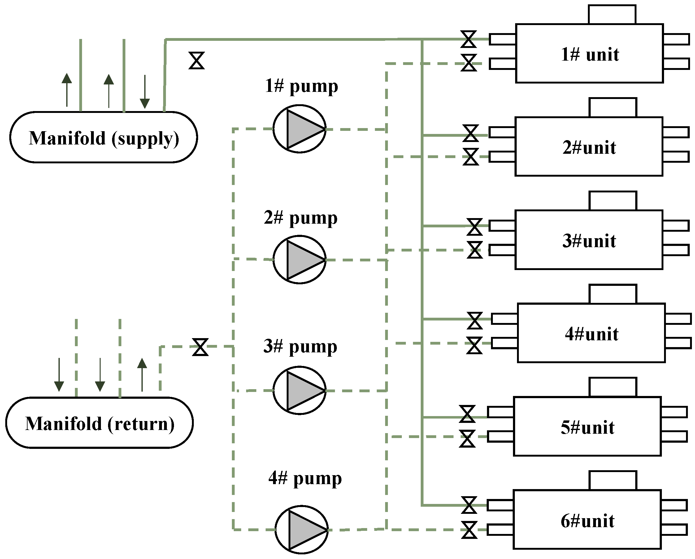
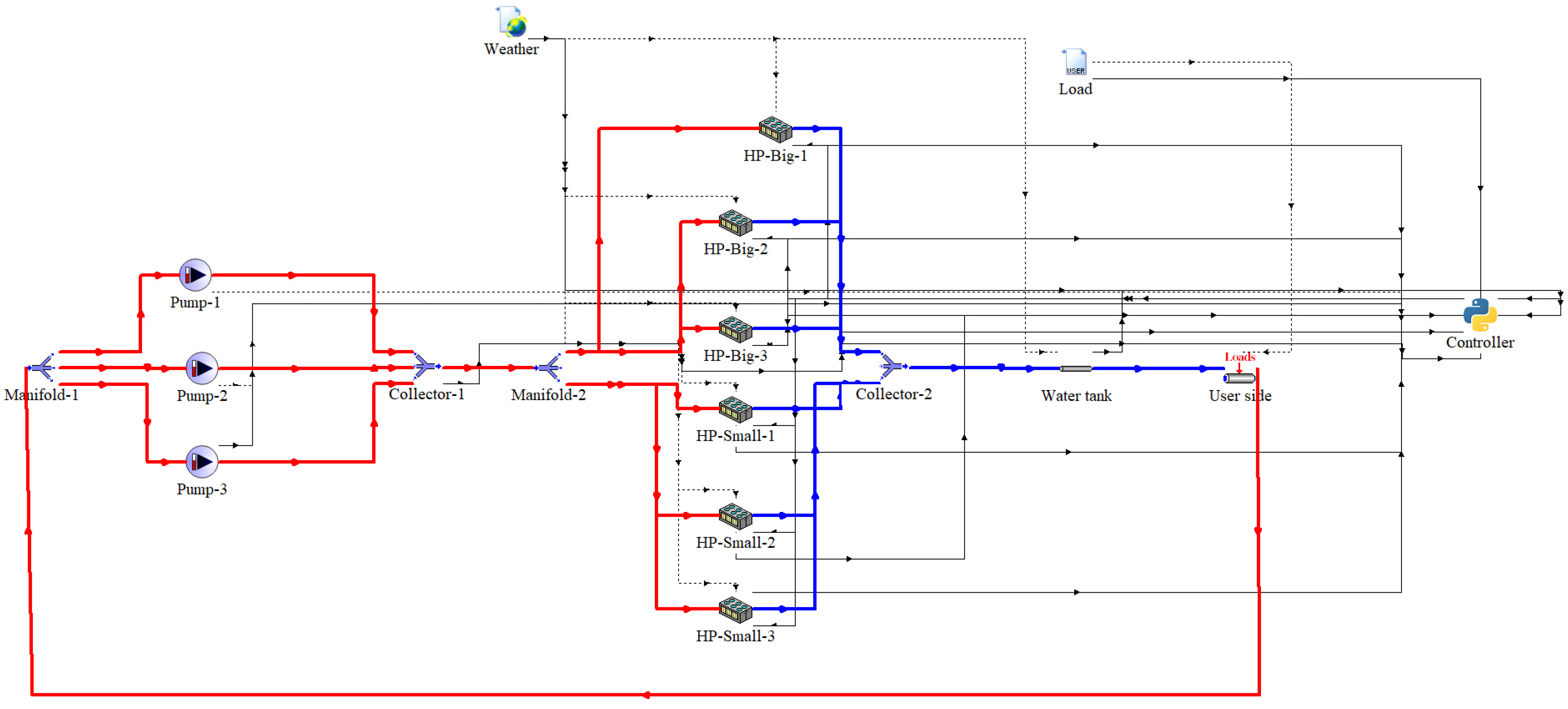
As shown in Figure 1, the system investigated in this study is a heterogeneous parallel air-source heat pump plant consisting of three large-capacity units, three small-capacity units, and a water-side pumping system. The main equipment parameters are summarized in

Table 1. Main parameters of the investigated heterogeneous air-source heat pump plant.

Device Type	Character	Count
Air cooled heat pump (Large)	Rated cooling capacity: 779 kW Rated power: 214 kW	3
Air cooled heat pump (Small)	Rated cooling capacity: 473 kW Rated power: 132 kW	3
Water pump	Rated power: 75 kW Rated flow: 236 m3/h	3 online 1 standby

. Since the units are arranged in parallel, the same cooling load can be satisfied by multiple combinations of large- and small-capacity units. Therefore, the system exhibits typical heterogeneous multi-unit regulation characteristics.

In conventional cooling plant supervisory control, unit staging is usually determined based on real-time operating variables, such as cooling load, supply-water temperature, return-water temperature, system PLR, and the operating status of each unit. To avoid frequent switching, staging thresholds are usually combined with persistence requirements, hysteresis bands, and minimum on/off-time constraints. Once an add-unit or remove-unit condition is satisfied, the controller selects the unit to be started or stopped according to a predefined sequence. After the active units are determined, the cooling load or water flow rate is usually distributed using fixed rules, such as equal-load, equal-flow, or capacity-proportional allocation.

This control structure is transparent, computationally inexpensive, and easy to implement in engineering practice. However, in a heterogeneous multi-unit system, it may restrict the flexible selection of unit combinations and may not sufficiently reflect the part–load efficiency differences among different units. Therefore, the limitations of conventional rule-based control are not only related to threshold parameters, but also to the feedback-triggered staging mechanism, predefined staging sequence, and fixed allocation rules.

2.2. Operational Deficiencies in Conventional Supervisory Control

Five observable operational deficiencies affect supervisory control of heterogeneous multi-unit cooling plants. They are associated with the interaction among active-unit selection, load allocation, and staging timing, and are reflected in energy efficiency, switching stability, and supply-water temperature reliability.

2.2.1. Feedback-Based Delayed Staging Response (D1)

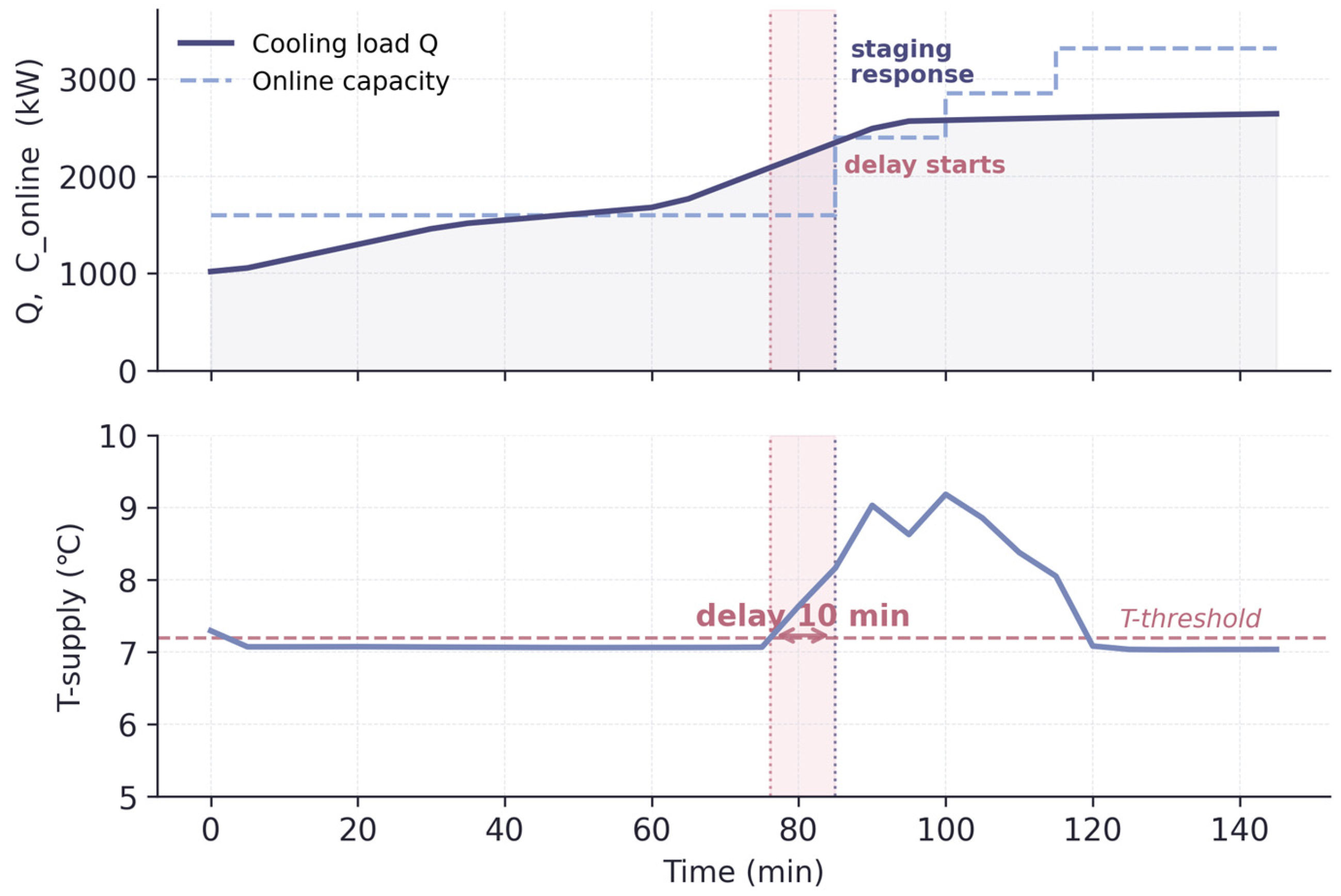
In conventional control, staging actions are triggered by current operating variables, such as unit PLR and supply-water temperature. To suppress chattering, the threshold condition must persist for a preset duration, and the add and remove thresholds form a hysteresis band. While this design improves stability, it inevitably introduces a delay between load variation and staging response.

During a rising load phase as shown in Figure 2, the active units may reach the full-PLR boundary and the supply water temperature gradually exceeds the set value. However, additional units are not started until the persistence requirement is satisfied. The delayed staging by this feedback regulation will lead to unstable water supply temperature and deviation of the equipment units from the optimal operating range.

2.2.2. Rigid Load Distribution Strategy (D2)

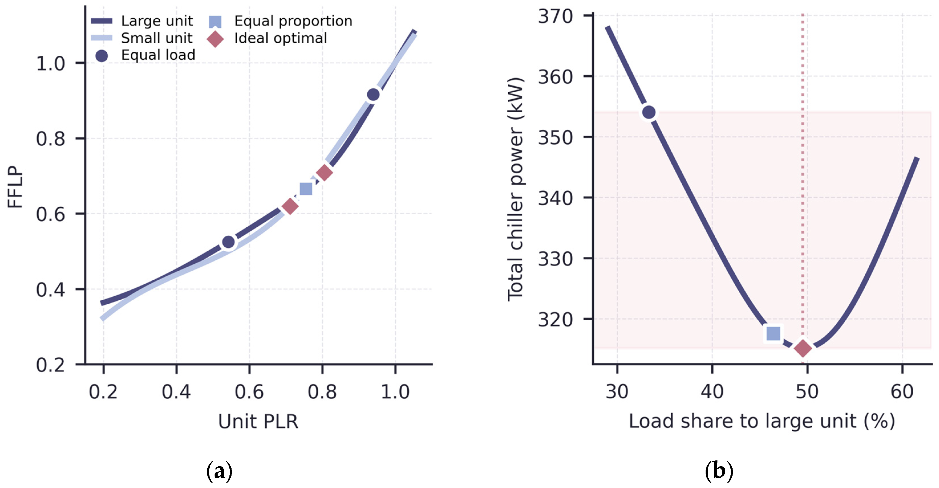
Once the unit combination is determined, the conventional control method distributes the cooling load through static rules, typically equal-load or capacity-proportional (equal-PLR) allocation. However, these rules cannot reflect the part–load efficiency characteristics of heterogeneous units. Under equal-load allocation, two units carrying the same load q satisfy

$$PL{R}_i={\displaystyle \frac{q}{C_i}},\hspace{1em}\hspace{1em}PL{R}_{\mathrm{j}}={\displaystyle \frac{q}{C_{\mathrm{j}}}}$$

(1)

Figure 3 compares three allocation strategies using a representative combination of one large unit and two small units. Under equal-load allocation, the large unit is pushed into a low-PLR, low-FFLP region, while the small units operate at moderate PLR (Figure 3a) and the corresponding point in Figure 3b sits at a large-unit share of only about 33%, which is well above the minimum power. Capacity-proportional allocation forces all units to the same PLR, but this common point does not coincide with the best-efficiency region of either fraction of full-load power (FFLP) curve; it only approaches the minimum-power point in Figure 3b. The ideal optimum, located near a 50% large-unit share, jointly minimizes total power on the two FFLP curves and can only be identified by accounting for the differences in their shapes.

Both rules are therefore static and ignore unit-level marginal efficiency. Relevant indicators include unit-level PLR distributions, branch-flow ratios, the small-to-large PLR ratio, and the relationship between load-share allocation and total chiller power.

2.2.3. Restricted Combination Access Under Fixed Staging Sequence (D3)

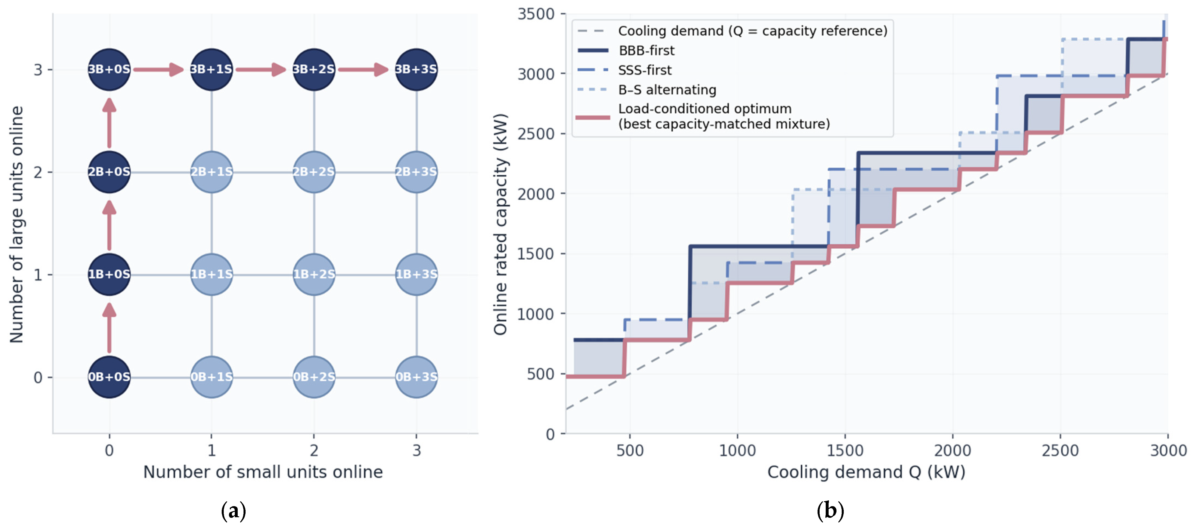
In a heterogeneous multi-unit plant, the same cooling demand can typically be met by several unit combinations. Each combination carries a different total online capacity and a different distribution of unit-level PLR under the same load distribution strategy. A fixed-sequence rule-based controller reduces this load-conditioned selection problem to movement along a predetermined staging path. Figure 4a illustrates this restriction in the combination space. A fixed staging sequence connects only a subset of combinations along a single chain. The remaining combinations are reachable in principle by a single unit transition but are excluded from the trajectory. Figure 4b shows the corresponding load-conditioned view across the operating range. The load-conditioned optimum, defined as the smallest capacity-feasible mixture at each demand, does not follow any single sequence. Different fixed sequences attain it in different load segments and depart from it elsewhere.

The central problem of D3 is that at every load condition rule-based control takes only one fixed staging sequence, and the controller can remain in an unfavorable combination even when better-matched alternatives are feasible.

2.2.4. Low-Efficiency Redundant Operation (D4)

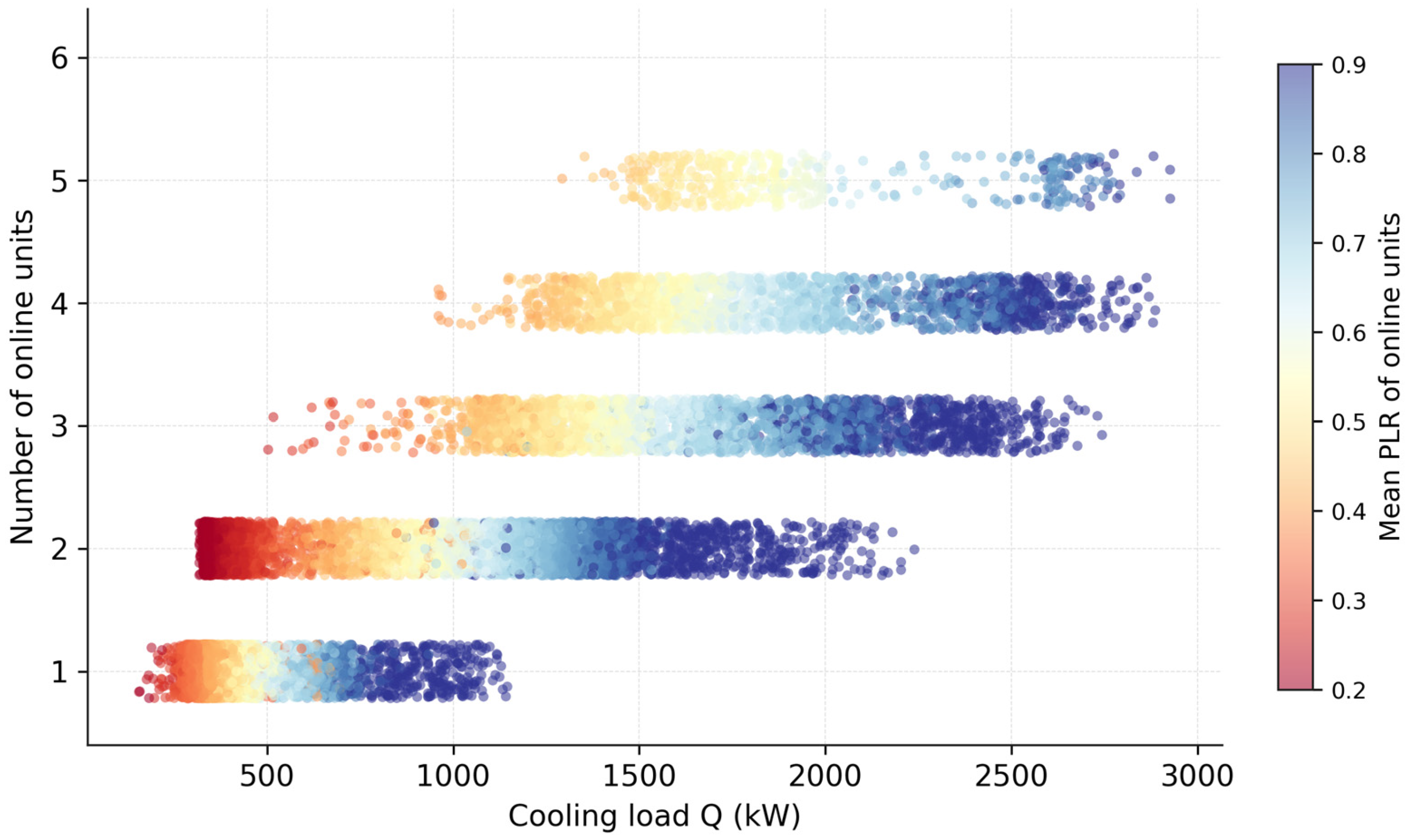
Following a peak-load period, the active unit count may not be reduced promptly, because the removal threshold is set conservatively or its persistence condition has not yet been satisfied. The available capacity then exceeds actual demand by a large margin, and each active unit operates at a low PLR. Figure 5 shows the distribution of the active unit count and corresponding mean PLR under a conventional RBC strategy. At a given cooling load, the mean PLR decreases markedly as the active unit count rises, confirming that conservative removal logic frequently keeps redundant units online. The contrast is most pronounced below 1000 kW: two-unit configurations operate within the efficient PLR range of 0.6–0.9, whereas four- and five-unit configurations covering the same load cluster below 0.4. A similar but weaker gap persists across the mid- and high-load regions. Once the active set fails to contract in step with falling demand, redundant units distribute the load across more devices than necessary, suppressing unit-level PLR and depressing plant-level efficiency.

This deficiency can be evaluated through the online unit count, the reserve margin, the low-PLR ratio, the efficient-PLR ratio, and the plant-level energy efficiency ratio.

2.2.5. Myopic Staging Without Trajectory-Level Action Evaluation (D5)

Some supervisory strategies pursue higher part–load efficiency or greater combination flexibility by making staging decisions from the current operating state alone, without evaluating whether the immediate energy benefit of an action will persist over the following control intervals. This absence of forward-looking information and trajectory-level evaluation produces two characteristic manifestations.

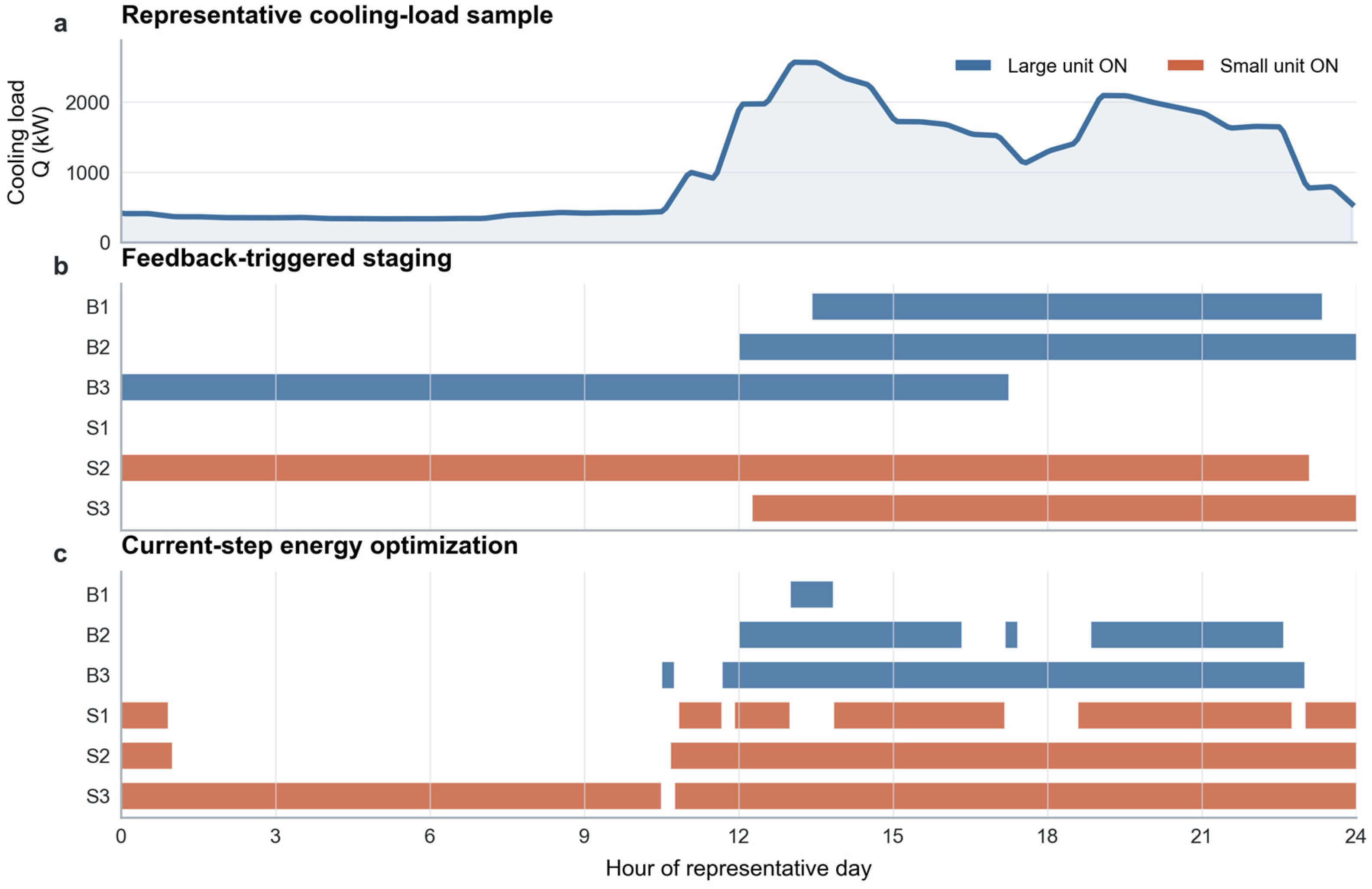
At the daily scale, the limitation appears as frequent movement between neighboring combinations. Figure 6 compares two representative control paradigms under the same 24 h load sample. The feedback-triggered paradigm completes the day with six unit-level switches by holding the active set across long intervals between major load changes. In contrast, the current-step energy-optimizing paradigm repeatedly follows load variations across low-power combination boundaries and accumulates 26 unit-level switches, including 10 switches on one small unit near the active-combination boundary. Thus, instantaneous energy optimization does not eliminate the energy-switching trade-off; it shifts the controller toward lower running power at the expense of switching stability.

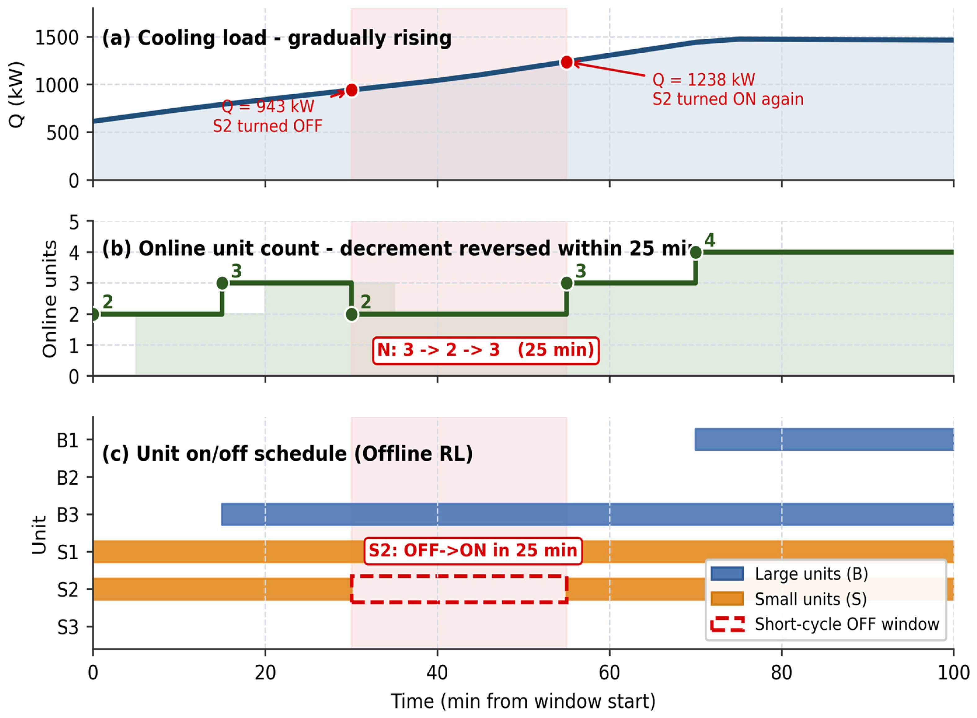
At shorter time scales, the same mechanism can produce rapid repeated on/off reversals, as illustrated in Figure 7. A unit may be stopped when the load briefly drops and restarted shortly after the load rises again, or the reverse may occur. Such short-time reversals indicate that an earlier transition is overturned before its operating benefit has been sustained long enough to justify the switching burden. D5 is therefore not merely a matter of threshold tuning, but a structural limitation of supervisory strategies that do not evaluate staging trajectories and their cumulative consequences.

2.3. Coupling Relationships Among the Operational Deficiencies

The operational deficiencies described above originate from two related sources: the decomposition logic of conventional rule-based control and the absence of trajectory-level evaluation in current-step supervisory strategies. In a heterogeneous multi-unit cooling plant, supervisory control is a mixed-discrete decision problem involving active-unit selection, load allocation, and transition evaluation under load variation. Rule-based control replaces this joint decision with a sequential rule chain: feedback triggering, priority-based unit transition, and static load allocation. This structure explains the delayed response, restricted combination usage, redundant operation, and rigid allocation observed in conventional control. By contrast, myopic staging arises when a supervisory strategy evaluates only the current-step benefit of a transition without considering its persistence or cumulative consequence.

The first structural separation is temporal. In rule-based control, hysteresis bands and persistence constraints make staging actions depend on delayed confirmation of the current state rather than on the expected consequence of near-future load evolution. This mechanism may be insufficient during rising-load periods and overly conservative during falling-load periods. However, removing these constraints or replacing them with current-step energy optimization does not eliminate the temporal problem; it may instead produce frequent reversals when the load fluctuates near a combination boundary.

The second separation is spatial. A heterogeneous plant may provide many feasible large-small unit mixtures under the same cooling load, but a fixed priority sequence reduces this combinatorial space to a narrow-ordered path. The next active set is therefore determined by rule reachability rather than by comparative evaluation among feasible combinations, limiting the use of capacity heterogeneity.

The third separation is objective-related. After the active set is determined, equal-load, equal-flow, or equal-PLR rules distribute load without evaluating the marginal power response of different unit types. Conversely, an improved loading rule can optimize the current active set, but it cannot determine whether another combination would yield lower cumulative cost over subsequent control intervals.

These limitations indicate that supervisory control should be reformulated as a trajectory-level selection problem. A suitable controller should compare feasible unit combinations, evaluate each combination through marginal-efficiency load allocation, and consider both operating cost and transition cost over a short future horizon.

3. The Scenario-Driven Marginal-Efficiency Graph Search Method

3.1. Overall Framework

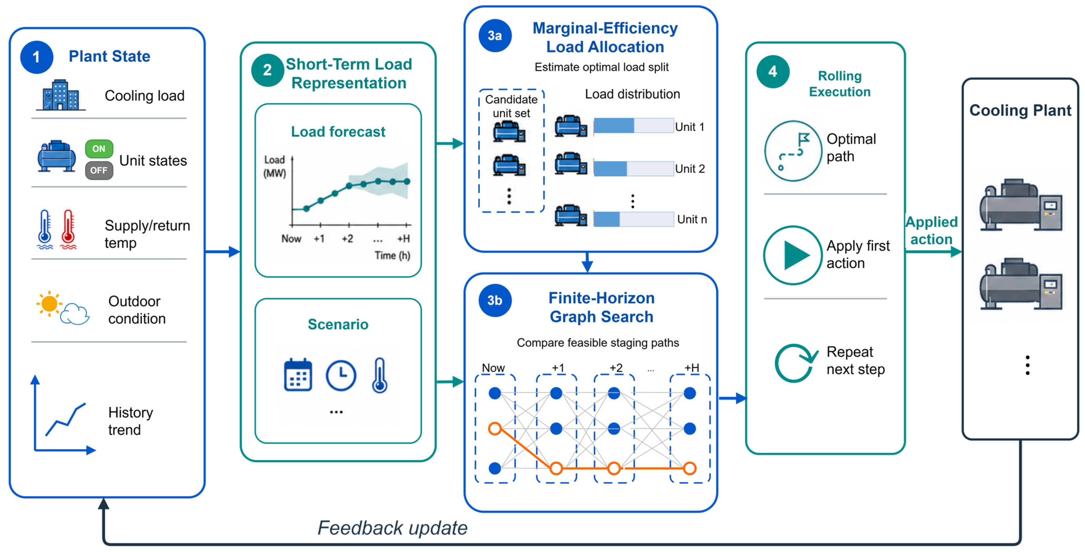
Based on the limitations identified in Section 2, this study proposes a scenario-driven marginal-efficiency graph search method, denoted as S-ME-GS, for supervisory control of heterogeneous multi-unit cooling plants. The method reformulates supervisory control from a one-step threshold-triggered decision into a rolling finite-horizon path-selection problem. As shown in Figure 8, the workflow consists of four stages: plant-state acquisition, short-term load representation, coupled decision evaluation, and rolling execution.

At each control step, the controller first receives the current plant state, including cooling load, unit on/off states, supply and return water temperatures, outdoor condition, and recent load history. These measurements provide the feedback basis for updating the control problem. The second stage constructs short-term load representation and operating-scenario information, which introduces forward-looking demand information into the decision process rather than relying solely on current feedback variables.

The third stage is the core decision layer and contains two coupled components. For each candidate active-unit set, the marginal-efficiency allocation module estimates the load distribution that minimizes operating power under admissible PLR constraints. This produces an efficiency-aware operating cost for each candidate combination. The finite-horizon graph-search planner then represents candidate unit combinations as nodes in a layered action graph and feasible hold, start, stop, or swap actions as edges. The planner compares staging paths using both node costs, such as energy and reserve adequacy, and edge costs, such as switching and transition penalties.

The final stage implements the rolling execution logic. After the minimum-cost future path is obtained, only the first action is applied to the cooling plant. The remaining path is used only to evaluate the current decision and is discarded at the next control step, when updated plant measurements and load information are received. Through this receding-horizon process, S-ME-GS links feedback updates, forward-looking load information, efficiency-aware allocation, and path-level staging evaluation within an interpretable supervisory-control structure.

3.2. Short-Term Load Representation and Operating Scenario Identification

The information module provides the graph-search planner with two inputs: a probabilistic short-term load trajectory and an operating-scenario label. The load trajectory describes future cooling demand over the planning horizon, whereas the scenario label summarizes the recent and near-future load-evolution pattern and adjusts the prediction envelope and path-cost preferences.

At each control step t, the forecaster receives a rolling historical operating sequence with L = 24 control steps, corresponding to 2 h at the 5-min supervisory interval. Each input vector contains five measured variables: cooling load, supply-water temperature, return-water temperature, total chilled-water flow rate, and outdoor air temperature. The historical input sequence is written as

$${\mathrm{X}}_t=\left[{\mathrm{x}}_{t-L+1},{\mathrm{x}}_{t-L+2},\dots ,{\mathrm{x}}_t\right],$$

(2)

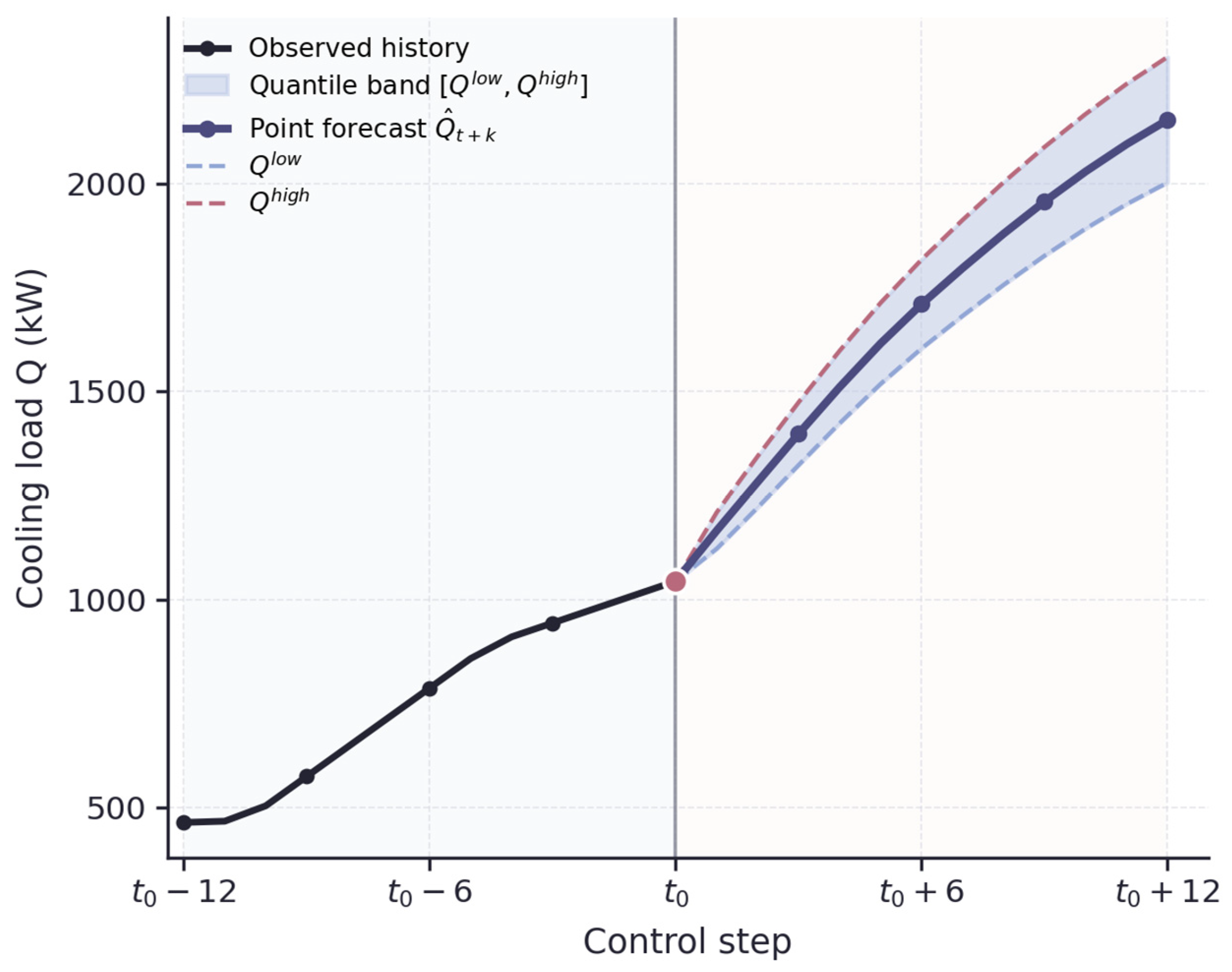
where ${\mathrm{x}}_t=\left[Q_t,T_t^{sup},T_t^{ret},G_t,T_t^{air}\right]$. $Q_t$ denotes the cooling load, $T_t^{sup}$ and $T_t^{ret}$ are the supply- and return-water temperatures, $G_t$ is the total chilled-water flow rate, and $T_t^{air}$ is the outdoor air temperature. A temporal convolutional network (TCN) generates the point load forecast for the next H = 12 control steps, corresponding to a 60-min look-ahead.

The forecaster produces a point load trajectory ${\hat{\mathrm{Q}}}_{t+1:t+H}=\left[{\hat{Q}}_{t+1},\dots ,{\hat{Q}}_{t+H}\right]$. To represent uncertainty, the residual distribution on the held-out set is used to construct lead-time-dependent quantile trajectories.

$$Q_{t+k}^{low}={\hat{Q}}_{t+k}+{\beta }_{s_t}{r}_k^{low}$$

(3)

$$Q_{t+k}^{base}={\hat{Q}}_{t+k}$$

(4)

$$Q_{t+k}^{high}={\hat{Q}}_{t+k}+{\beta }_{s_t}{r}_k^{high},k=1,\dots ,H$$

(5)

where $r_k$ is the empirical p-quantile of the forecast residual at lead time k and ${\beta }_{s_t}$ is the prediction-envelope scaling factor under the current operating scenario. The base trajectory estimates the expected operating cost, the high trajectory evaluates reserve adequacy and shortage risk, and the low trajectory helps identify redundant online capacity. These three trajectories form a synchronized uncertainty envelope of the same future demand process.

In this study, the TCN is used as the load-information module that provides the graph-search planner with a point forecast and an empirical residual-quantile envelope. The main controller therefore depends on the forecast output and uncertainty representation rather than on a specific forecasting architecture.

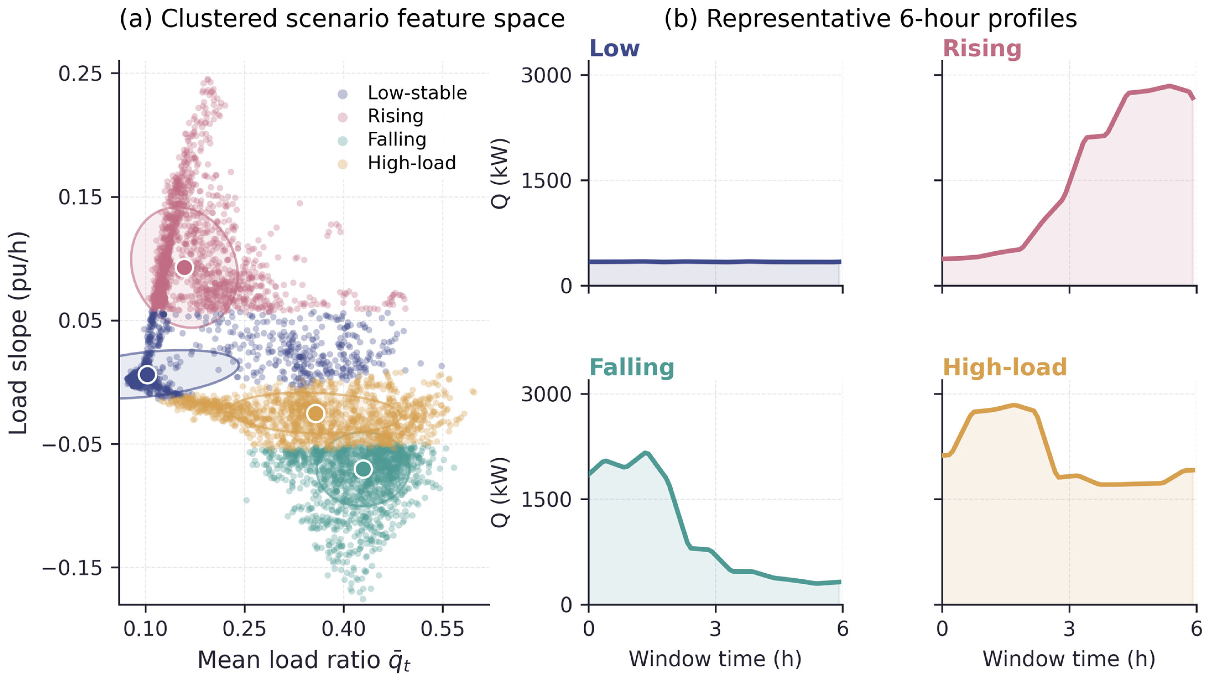
The operating scenario is identified separately from the quantile trajectories. It is derived from the recent load window and the point forecast using three interpretable indicators: mean load ratio, average load slope, and fluctuation intensity. These categories capture the main control-relevant patterns of plant operation. Rising-load and high-load periods require stronger reserve protection, whereas low-load and falling-load periods require greater attention to redundant online capacity and low-PLR operation. Figure 9 illustrates one representative historical input window and the corresponding point and quantile load trajectories used by the planner.

In this study, feature clustering is performed for the investigated chiller plant, and the current operating scenario is identified by combining historical load and predicted load information:

$$s_t=\mathcal{C}\left({\mathrm{Q}}_{t-L:t},{\hat{\mathrm{Q}}}_{t+1:t+H},{\mathrm{z}}_t\right)$$

(6)

where ${\mathbf{z}}_t$ denotes auxiliary variables such as outdoor temperature, time-related features, or other operational descriptors. Four operating scenarios are considered:

$$s_t=\in \left\{S_1^{low},S_2^{rising},S_3^{falling},S_4^{high}\right\}$$

(7)

Here, $S_1^{low}$ denotes a low-load scenario, $S_2^{rising}$ denotes a rising-load scenario, $S_3^{falling}$ denotes a falling-load scenario, and $S_4^{high}$ denotes a high-load scenario. The operating scenario is used to characterize the load-evolution pattern within the current rolling horizon and to provide scenario information for prediction-envelope adjustment and path-cost evaluation. Since the controller updates the forecast and re-identifies the operating scenario at every control step, the scenario label evolves dynamically with the load trajectory. Figure 10 shows the clustered scenario feature space and representative load profiles used to interpret the four operating scenarios.

The deployed load-representation module was documented using the architecture and inference settings in Appendix A,

Table A1. Deployed TCN load-forecasting module configuration.

Item	Setting Used in This Study
Model role	Short-term sequence load forecaster used by the S-ME-GS information module
Model type	TCN sequence model (tcn_seq) exported to ONNX
Input shape	[batch, 24, 5]
Input variables	Q, T-supply, T-return, G, and T-air
Output shape	[batch, 12] point load trajectory
Temporal blocks	Two residual temporal convolution blocks
Hidden channels	64
Convolution setting	Kernel size 3, stride 1, dilation factors 1 and 2
Downsampling	1 × 1 convolution from 5 to 64 channels in the first block
Prediction head	Linear 64-64-ReLU followed by Linear 64-12
Training split and settings	70/15/15 train/validation/test split; 80 epochs; batch size 256; learning rate 1 × 10−3; weight decay 1 × 10−5; early-stopping patience 12
Uncertainty envelope	Lead-time residual quantiles added to the point forecast

and

Table A2. Forecast error summary of the TCN forecaster.

Horizon	N	MAE (kW)	RMSE (kW)	MAPE (%)	NMAE (%)
5 min	26,495	27.137	40.876	5.07	2.89
30 min	26,490	93.637	154.553	12.43	9.97
60 min	26,484	154.275	236.319	19.69	16.42

, documents the architecture, inference settings, and lead-time forecasting errors of the deployed load-representation module.

3.3. Marginal-Efficiency Load Allocation

For a heterogeneous multi-unit cooling plant, the same cooling load can be satisfied by different combinations of large- and small-capacity units. These combinations differ in online capacity, unit-level PLR distribution, and energy consumption. S-ME-GS therefore evaluates each candidate combination using marginal-efficiency load allocation rather than equal-load, equal-flow, or capacity-proportional rules.

$\mathbf{u}$ denotes a candidate unit combination, and $\mathcal{A}\left(\mathbf{u}\right)$ denotes the set of online units. For online unit $i$, let $q_i$ be the assigned cooling load and $C_i$ be the rated cooling capacity. The part–load ratio and the power model are written as

$$P_i\left(q_i\right)=P_i^{rated}{f}_i\left({\mathrm{P}\mathrm{L}\mathrm{R}}_i\right)$$

(8)

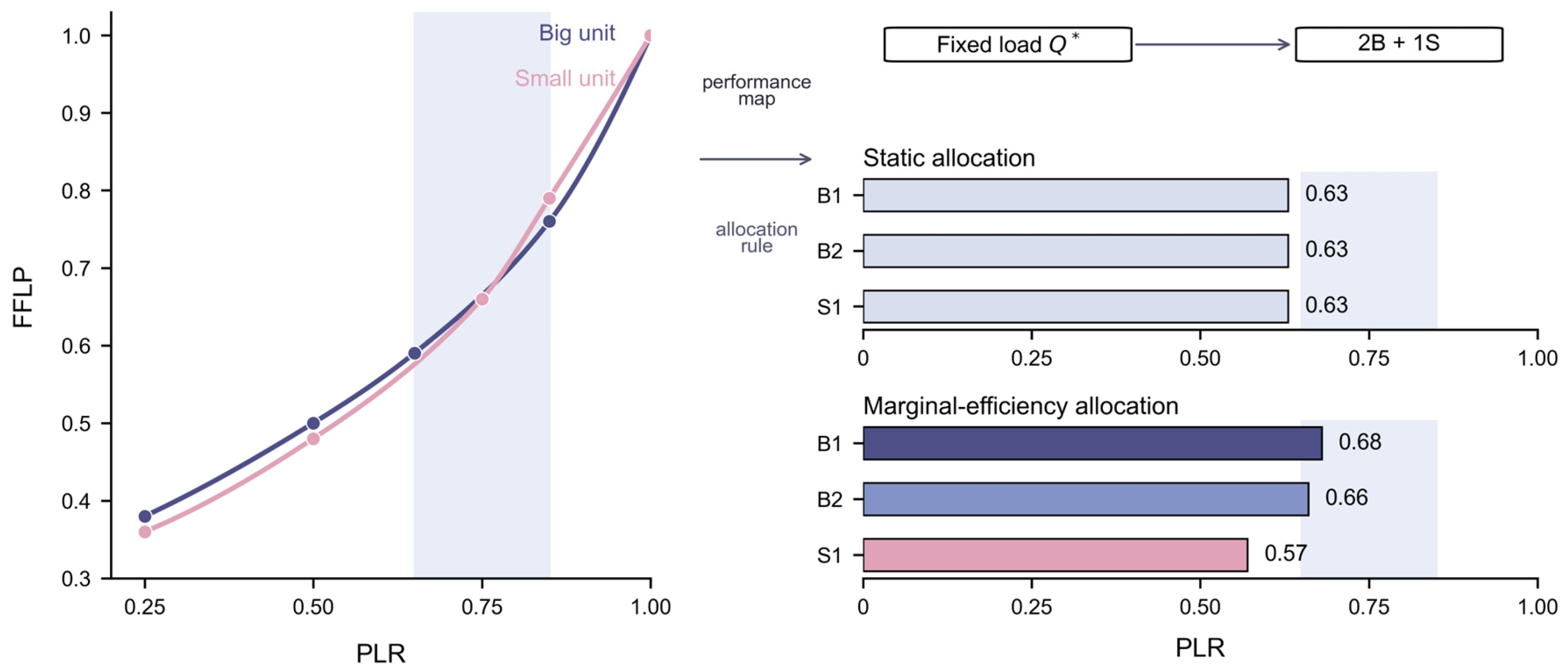
Here, $P_i^{rated}$ denotes the rated power, and $f_i\left(\cdot \right)$denotes the PLR–FFLP performance curve of unit $i$. This curve can be obtained from manufacturer data, experimental fitting, or interpolation of discrete performance points. Since different unit types have different capacities, rated COPs, and part–load performance curves, the marginal electric cost may differ even under the same PLR or the same load fraction. This provides the basis for using marginal-efficiency allocation rather than static allocation rules.

For a given cooling load $Q$ and candidate combination $\mathbf{u}$, the load allocation problem is formulated as

$$\underset{q_i}{\min }\sum _{i\in \mathcal{A}\left(\mathbf{u}\right)}{P}_i\left(q_i\right)$$

(9)

subject to

$$\sum _{i\in \mathcal{A}\left(\mathbf{u}\right)}{q}_i=Q,\hspace{1em} q_i^{min}\le q_i\le q_i^{max},$$

(10)

where $q_i^{min}$ and $q_i^{max}$ are determined by the allowable lower and upper PLR bounds of unit $i$.

Within the operating range considered in this study, the chiller power curves are approximated by convex piecewise functions. Under this approximation, the allocation problem can be solved as a constrained convex optimization problem with one linear equality constraint and box constraints. For online units that do not reach their PLR bounds, the first-order optimality condition is

$${\displaystyle \frac{\partial P_i\left(q_i^{\mathrm{*}}\right)}{\partial q_i}}{=\lambda }^{\mathrm{*}},i\in {\mathcal{A}}^{free}\left(\mathbf{u}\right)$$

(11)

Here, ${\lambda }^{*}$ is the Lagrange multiplier associated with the load–balance constraint, and ${\mathcal{A}}^{free}\left(\mathbf{u}\right)$ denotes the set of online units that do not reach their operating bounds. This condition indicates that the optimal allocation does not require equal load or equal PLR across units. Instead, it equalizes the marginal electric cost of all unconstrained online units. When a unit reaches its upper or lower PLR bound, its load is determined by the corresponding boundary constraint, and the remaining load is allocated among the other feasible units. Figure 11 illustrates this marginal-efficiency allocation process under a fixed load and active-unit combination.

The marginal-efficiency allocation returns the optimal load distribution $q^{*}\left(u,Q\right)$, the corresponding PLR distribution, and the total chiller power:

$$P_{ch}\left(\mathbf{u},Q\right)=\sum _{i\in \mathcal{A}\left(\mathbf{u}\right)}{P}_i\left(q_i^{\mathrm{*}}(u,Q)\right)$$

(12)

In addition to chiller power, the plant-level evaluation also includes the pump power associated with the active combination and the required chilled-water flow. In a general form, the pump power is expressed as

$$P_{\mathrm{p}\mathrm{u}\mathrm{m}\mathrm{p}}\left(\mathbf{u},Q\right)={\Phi }_p\left(G\left(\mathbf{u},Q\right),N_{\mathrm{o}\mathrm{n}}^p\left(\mathbf{u}\right)\right),$$

(13)

where $G\left(\mathbf{u},Q\right)$ is the flow required by the allocated cooling load, $N_{\mathrm{o}\mathrm{n}}^p\left(\mathbf{u}\right)$ is the number of active pumps, and ${\Phi }_p\left(\cdot \right)$ represents the pump-power model. Depending on the available plant information, ${\Phi }_p\left(\cdot \right)$ can be represented by a calibrated empirical model or by a system-curve-based variable-frequency pump model. The total plant power used in the graph-search evaluation is therefore

$$P_{\mathrm{t}\mathrm{o}\mathrm{t}}\left(\mathbf{u},Q\right)=P_{\mathrm{c}\mathrm{h}}\left(\mathbf{u},Q\right)+P_{\mathrm{p}\mathrm{u}\mathrm{m}\mathrm{p}}\left(\mathbf{u},Q\right)$$

(14)

This procedure maps each feasible unit combination to a consistent operating evaluation under a given load, including the optimal load distribution, unit-level PLR, chiller power, pump power, and total plant power. Marginal-efficiency allocation therefore serves as an evaluation module rather than a staging controller; it converts each candidate combination into a comparable node for the predictive graph search.

3.4. Predictive Action Graph and Path-Cost Formulation

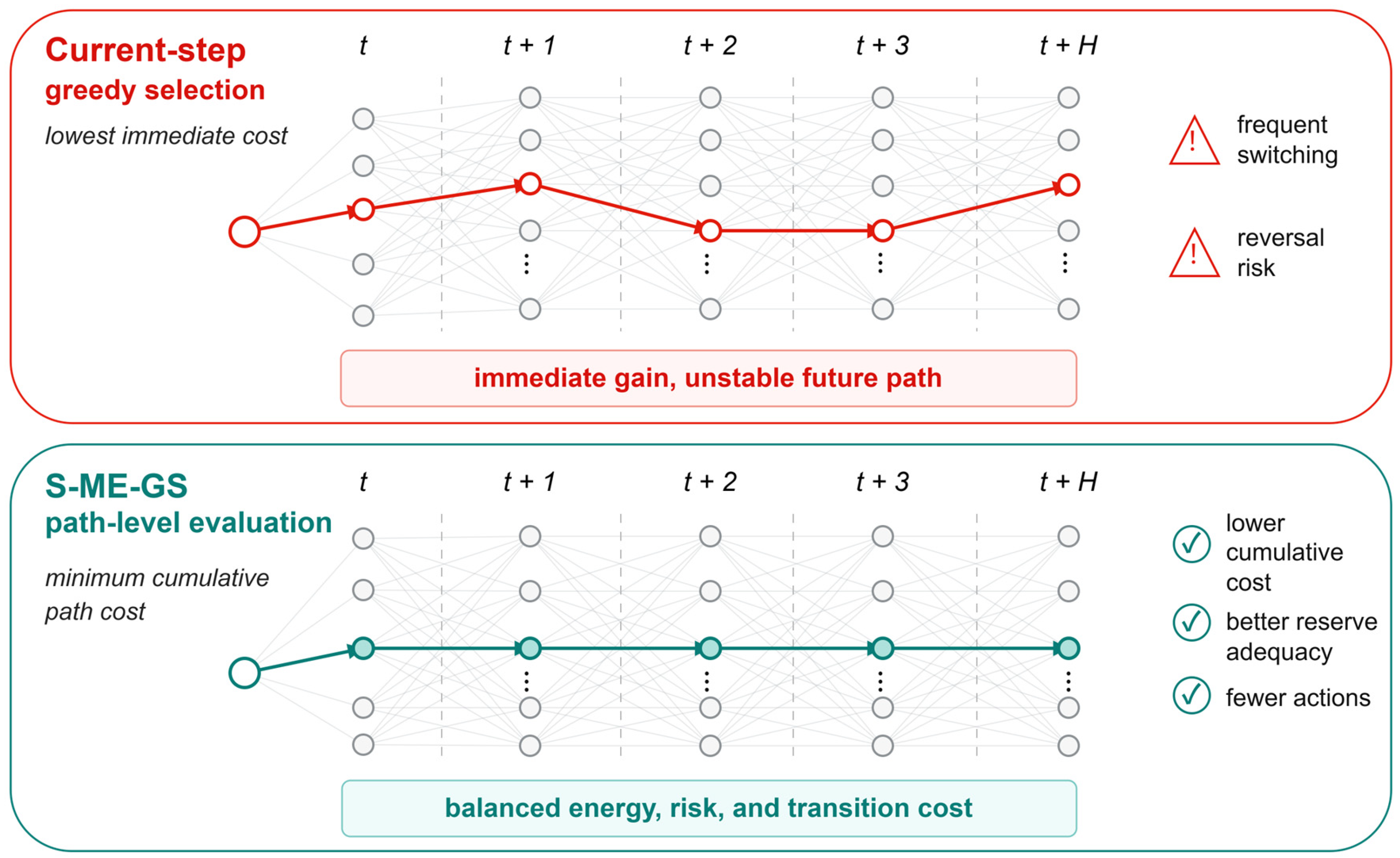
The staging decision of a multi-unit cooling plant exhibits temporal coupling. The current combination affects immediate power consumption, reserve capacity, feasible future transitions, and switching burden. Selecting only the current minimum-power combination can therefore produce unstable trajectories near combination boundaries.

Figure 12 illustrates the difference between current-step greedy selection and path-level evaluation. A greedy strategy follows the immediate minimum-cost combination, but locally optimal decisions may cause repeated switching, insufficient reserve, or higher cumulative transition burden. S-ME-GS instead compares feasible combination paths over the prediction horizon and minimizes cumulative energy, reserve-risk, and transition costs while executing only the first accepted action.

S-ME-GS formulates supervisory staging as a finite-horizon combination-path selection problem, but the candidate set is constructed online from the current operating state instead of enumerating a full Cartesian product. The predictive action graph is layered by future control step. Each node represents a retained active-unit combination, and each edge represents a feasible hold, start, stop, or swap transition between adjacent layers. Algorithm 1 summarizes the layered dynamic-programming implementation of the predictive action graph.

Algorithm 1. Layered dynamic-programming implementation of the predictive action graph.
Step	Operation
1	Read the current active-unit combination, measured load, lockout counters, and low, base, and high load trajectories.
2	Generate the first graph layer from the hold action and feasible one-step neighboring actions, including start, stop, and swap transitions from the current combination.
3	At each later horizon layer, expand only the retained states from the previous layer and discard candidates that violate capacity, PLR, lockout, staging-interval, or single-step action constraints.
4	For each remaining candidate node, run marginal-efficiency allocation under the low, base, and high trajectories, and compute the node-level energy and reserve-risk terms.
5	Propagate cumulative path costs by adding transition costs to the discounted node costs, then retain only the lowest-cost beam and store predecessors.
6	Select the terminal state with the smallest cumulative cost and reconstruct the best path.
7	Compare the best path with the hold-current path, and execute its first future action only when the improvement exceeds the scenario-dependent activation margin.

Although six units imply 64 binary states, the planner does not enumerate all H-step state sequences. Starting from the current combination, each layer expands only feasible hold, start, stop, or swap neighbors from the states retained at the previous layer. Capacity, PLR, minimum on/off time, staging-interval, and single-step action constraints are applied before cost propagation. The resulting retained path over the planning horizon is represented as

$${\mathcal{P}}_t=(u_t,u_{t+1},\dots ,u_{t+H}),$$

(15)

Here, the feasible path set is generated recursively from the current combination. It contains the retained neighbor paths used by the layered planner, rather than every possible combination sequence across the horizon.

At each candidate node, the marginal-efficiency allocator computes the minimum-power load distribution under the low, base, and high load trajectories. The node cost combines expected plant energy and reserve-shortage risk, while hard capacity and PLR constraints are screened before cost propagation. The edge cost represents the operational burden of transitions between adjacent combinations, including starts, stops, swaps, and other transition-related action features.

After each layer, beam pruning retains only the lowest-cost states. The beam width is eight in this study, which preserves a small set of alternative feasible trajectories while limiting online computation. For every retained path, the cumulative path cost is evaluated by adding future node costs and transition burdens over the horizon:

$$J\left({\mathcal{P}}_t\right)={\displaystyle \sum _{k=1}^H}{\gamma }^{k-1}\hspace{0.17em}{C}_{node}\left(u_{t+k}\right)+{\displaystyle \sum _{k=1}^H}{C}_{edge}(u_{t+k-1}, u_{t+k}),$$

(16)

where $\gamma \in (0, 1]$ is the temporal discount factor, $C_{node}$ is the node operating cost, and $C_{edge}$ is the transition cost between adjacent combinations. The discount factor is applied to the node term to reflect the decreasing confidence of the load prediction with lead time, but not to the edge term, since the physical cost of an action does not depend on when it occurs along the horizon.

The node cost is formulated as

$$C_{node}\left(u_{t+k}\right)=E\left(u_{t+k}\right)+{\alpha }_R^{\left(s_t\right)}\hspace{0.17em}R\left(u_{t+k}\right),$$

(17)

where $E\left(\cdot \right)$ is the scenario-weighted operating-energy term, $R\left(\cdot \right)$ is the reserve-risk term, and ${\alpha }_R^{\left(s_t\right)}$ is the scenario-dependent reserve-risk weight under the current operating scenario $s_t$.

The operating-energy term is defined as

$$E\left(u_{t+k}\right)=\sum _{\xi \in \left\{low\hspace{0.17em}base\hspace{0.17em}high\right\}}{w}_{\xi }^{\left(s_t\right)}\left[P_{ch}(u_{t+k},{\widehat{Q}}_{t+k}^{\xi })+P_{pump}(u_{t+k},{\widehat{Q}}_{t+k}^{\xi })\right]\mathsf{\Delta }t,$$

(18)

where ${\widehat{Q}}_{t+k}^{\xi }$ denotes the predicted cooling load at the $k$-th future step under trajectory $\xi$, $w_{\xi }^{\left(s_t\right)}$ is the corresponding scenario-dependent trajectory weight with ${\sum }_{\xi }{w}_{\xi }^{\left(s_t\right)}=1$, and $\mathsf{\Delta }t$ is the control interval. The chiller power $P_{ch}$ is obtained from the marginal-efficiency allocation of Section 3.3, and the pump power $P_{pump}$ follows from the resulting chilled-water flow under the active set. The node-level energy cost therefore reflects both the minimum-power internal load distribution and the hydraulic consequence of the active combination, integrated across the forecast uncertainty envelope.

The capacity-risk term evaluates the reserve adequacy of a candidate combination under the predicted load trajectories. Let the online capacity of a candidate combination be

$$C_{cap}\left(u_{t+k}\right)={\displaystyle \sum _{i=1}^N}{u}_{i,t+k}\hspace{0.17em}{C}_i.$$

(19)

The reserve-risk term is then defined as

$$R\left(u_{t+k}\right)=\sum _{\xi \in \left\{low\hspace{0.17em}base\hspace{0.17em}high\right\}}{w}_{\xi }^{\left(s_t\right)}{\left[\left(1+\rho \right)\hspace{0.17em}{\widehat{Q}}_{t+k}^{\xi }-C_{cap}\left(u_{t+k}\right)\right]}_{+},$$

(20)

where $\rho$ is the minimum reserve ratio and ${\left[x\right]}_{+}=\mathrm{m}\mathrm{a}\mathrm{x}(x,0)$. The risk term is evaluated under the same scenario-weighted trajectories as the operating-energy term, so that candidate combinations whose online capacity becomes insufficient under any plausible load realization are penalized in proportion to that trajectory’s weight. The term is zero when the candidate combination satisfies the reserve requirement under all three trajectories and grows with the weighted capacity deficit otherwise. This forward-looking reserve evaluation distinguishes S-ME-GS from the current-step ME-only reference, which does not evaluate path-level reserve adequacy.

The edge cost characterizes the operational burden of changing the active unit set between two adjacent control steps. It depends jointly on $u_{t+k-1}$ and $u_{t+k}$ and is written as

$$C_{edge}(u_{t+k-1},u_{t+k})=\sum _j{\alpha }_j^{\left(s_t\right)}\hspace{0.17em}{\varphi }_j(u_{t+k-1},u_{t+k}),$$

(21)

where ${\varphi }_j$ denotes the action features used to count the discrete operations that distinguish $u_{t+k-1}$ from $u_{t+k}$, including starts, stops, and one-for-one replacements. The coefficients ${\alpha }_j^{\left(s_t\right)}$ are the corresponding scenario-dependent weights, with units of kWh per action. A one-for-one replacement is treated as a single action feature rather than as a start plus a stop, because it preserves both the total online capacity and the chilled-water hydraulic state and therefore should not incur a double penalty.

The graph-search planner selects the path with the minimum total cost:

$${\mathcal{P}}_t^{*}=\arg \underset{{\mathcal{P}}_t\in {\Omega }_t}{\mathrm{m}\mathrm{i}\mathrm{n}}J\left({\mathcal{P}}_t\right)$$

(22)

Because S-ME-GS follows a rolling-horizon execution strategy, the controller does not execute the entire future path at once. Instead, only the first future action of the selected path is considered. To avoid frequent switching caused by marginal predicted benefits, an action activation margin is further introduced. Let ${\mathcal{P}}_t^{hold}$ denote the reference path that maintains the current combination. The cost improvement of the optimal path over the holding path is

$$\mathsf{\Delta }{J}_t=J\left({\mathcal{P}}_t^{hold}\right)-J\left({\mathcal{P}}_t^{\mathrm{*}}\right).$$

(23)

The final control command is

$$u_{t+1}^{cmd}=\{\begin{array}{cc}\mathrm{first}\left({\mathcal{P}}_t^{\mathrm{*}}\right),& \mathsf{\Delta }{J}_t\ge {ϵ}_{act}^{\left(s\right)},\\ u_t,& \mathsf{\Delta }{J}_t<{ϵ}_{act}^{\left(s\right)}.\end{array}$$

(24)

Here, ${ϵ}_{act}^{\left(s\right)}$ is the action activation margin under the scenario (units: kWh). The controller changes the current combination only when the selected switching path provides a sufficiently clear cumulative benefit over the holding path; otherwise, the current operating state is maintained. At the next control step, the controller re-collects system states, updates the forecast, re-identifies the operating scenario, and performs graph search again.

The resulting online workload is governed by the horizon length, the local neighbor degree, the retained beam width, and the number of marginal-efficiency allocation calls, rather than by exhaustive enumeration of all H-step binary sequences. In this study, the beam width is eight and only feasible one-step neighbors are expanded from retained states, so the candidate set remains small throughout the 12-step horizon. The function-level benchmark reported in Appendix A

Table A3. Function-level runtime benchmark of the layered graph-search planner.

Metric	Value
Sampled control steps	240
Mean runtime (ms)	85.319
Median runtime (ms)	70.893
95th percentile runtime (ms)	166.020
Maximum runtime (ms)	227.497
Maximum share of 5-min control interval (%)	0.075832

shows a mean planner runtime of 85.3 ms and a maximum runtime of 227.5 ms per control step, which is far below the 5-min supervisory interval. This timing result supports the real-time tractability of the tested implementation while remaining an implementation-level result for the studied plant configuration.

3.5. Calibration of Path-Cost Weights

The weights in the path-cost formulation were not tuned against the 62-day closed-loop evaluation results. Instead, they were calibrated offline using a chronologically preceding logged segment that was not included in the evaluation window. In this study, the calibration segment contains the first 2000 logged 5-min control steps, corresponding to approximately 7 days of operation.

The calibrated parameter set includes only supervisory decision weights:

$$\theta =\{w_{\xi }^{\left(s_t\right)},{\alpha }_R^{\left(s_t\right)},\left\{{\alpha }_j^{\left(s_t\right)}\right\},{ϵ}_{act}\}.$$

(25)

Scenario-dependent values are constructed from baseline coefficients and scenario-specific multipliers, so that adaptation across operating scenarios is represented compactly within a single parameter set.

For each candidate $\theta$, the controller performs a complete offline replay over the calibration segment under identical load, weather, and equipment conditions. The replay yields a multi-indicator performance vector, which is scalarized into a single calibration objective:

$$\mathsf{\Phi }\left(\theta \right)={\lambda }_E{\tilde{W}}_E+{\lambda }_S{\tilde{N}}_{sw}+{\lambda }_R{\tilde{\mathsf{\Delta }}}_R+{\lambda }_L{\tilde{L}}_{lp},$$

(26)

where ${\tilde{W}}_E$, ${\tilde{N}}_{sw}$, ${\tilde{\mathsf{\Delta }}}_R$, and ${\tilde{L}}_{lp}$ are the normalized total electricity consumption, switching count, capacity-shortage indicator, and low-PLR exposure, respectively. Bayesian optimization is used to search for

$${\theta }^{*}=\arg \underset{\theta \in \Theta }{\mathrm{m}\mathrm{i}\mathrm{n}}\mathsf{\Phi }\left(\theta \right),$$

(27)

where $\Theta$ is the parameter search space. The optimization was implemented using Optuna with a tree-structured Parzen estimator sampler. The obtained parameters were fixed before the 62-day closed-loop evaluation and were not adjusted according to the evaluation results. Appendix A Table A3 and

Table A4. Class-specific baseline action costs used in the edge-cost formulation.

Class	${\mathit{c}}^{\mathit{s}\mathit{t}\mathit{a}\mathit{r}\mathit{t}}$ (kWh)	${\mathit{c}}^{\mathit{s}\mathit{t}\mathit{o}\mathit{p}}$ (kWh)
Large (B)	40	15
Small (S)	25	8

list the calibrated values.

4. Experiment Evaluation and Discussion

4.1. Experimental Platform and Strategies Design

This study conducts closed-loop evaluations of the proposed S-ME-GS control method using a TRNSYS–Python co-simulation platform. TRNSYS is used to simulate the cooling plant and the dynamic response of the water-side loop, while Python implements the upper-level supervisory control logic. At each control interval, the controller reads the cooling load, supply and return water temperatures, total water flow rate, outdoor air temperature, and the operating state of each unit, and then sends the unit on/off commands and flow allocation ratios back to the simulation platform. The case study is based on the heterogeneous parallel air-source heat pump system introduced in Section 2, with its configuration and simulation mapping shown in Figure 13. The co-simulation was implemented using TRNSYS 18 and Python 3.11.

Five strategies were compared, as summarized in

Table 2. Control strategies used for performance comparison.

Strategy	Main Characteristic	Role in Comparison
RBC-A	Fixed-threshold control with a large-unit-first sequence	Conventional baseline
RBC-B	Fixed-threshold control with an alternative fixed sequence	Tests sensitivity to staging order
ME-only	Current-step marginal-efficiency decision	Tests one-step efficiency optimization
Offline RL	Data-driven state-to-combination policy	Learning-based baseline
S-ME-GS	Forecast-guided marginal-efficiency graph search	Proposed method

. Two fixed-sequence RBC strategies were used to represent conventional rule-based control under different staging orders. The ME-only strategy was included to evaluate the effect of current-step marginal-efficiency optimization. The offline RL strategy was used as a data-driven control baseline. The proposed S-ME-GS method was evaluated as the integrated strategy combining load scenarios, marginal-efficiency allocation, and finite-horizon graph search.

For a cooling plant control system, the objective is not merely to reduce energy consumption, but to coordinate energy efficiency, operational stability, and water-side thermal reliability while maintaining stable cooling supply. Therefore, this study evaluates the closed-loop operating performance of different control strategies from four aspects: cooling plant energy consumption, unit PLR distribution, unit switching stability, and water-side thermal reliability. The main evaluation metrics are summarized in

Table 3. Evaluation metrics for closed-loop operating performance.

Dimension	Main Metrics	Evaluation Purpose
Energy consumption	Total electricity consumption, chiller electricity consumption, pump electricity consumption	Compares overall energy-saving performance
PLR distribution	Low-PLR proportion, high-efficiency PLR proportion	Evaluates part–load operating quality and low-load redundant operation
Switching stability	Unit-level switching count, switching density	Quantifies control action frequency and equipment switching burden
Thermal reliability	Supply-temperature violation ratio, cumulative temperature exceedance	Evaluates the occurrence frequency, magnitude, and duration of supply-temperature violations

.

To ensure consistent comparison across different strategies, several metrics are further specified. The high-efficiency PLR range is determined according to the PLR–FFLP performance curves of the large- and small-capacity units, and is uniformly taken as 0.6 ≤ PLR ≤ 0.9 in this study. The unit-level switching count is accumulated according to changes in the on/off state of each individual unit, rather than merely by whether the overall unit combination changes. Switching density is defined as the unit-level switching count divided by the number of evaluation days. The supply-water temperature violation threshold is determined based on the 7.0 °C setpoint and a 5% engineering tolerance, giving a threshold of 7.35 °C. The cumulative temperature exceedance is used to jointly characterize the magnitude and duration of temperature violations.

4.2. Performance Comparison Among Different Control Strategies

4.2.1. Electricity Consumption and Combination Coverage

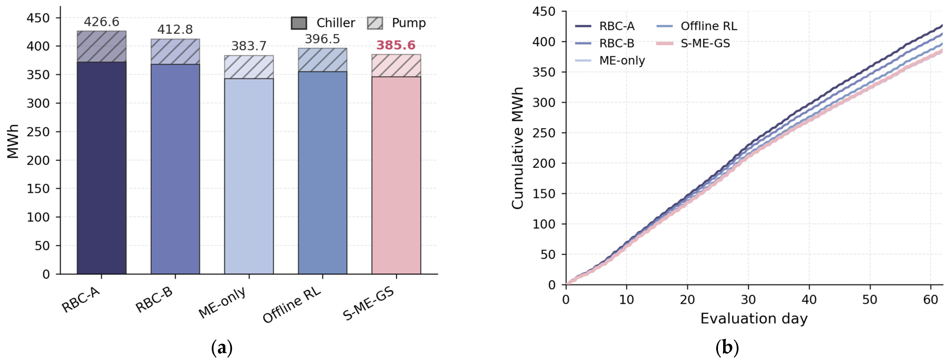
Total electricity consumption over the 62-day evaluation period ranges from 383.7 MWh for ME-only to 426.6 MWh for RBC-A, corresponding to an 11.2% spread across the five control strategies.

RBC-B consumes 412.8 MWh, which is 3.23% lower than RBC-A, although the two RBC strategies use the same threshold logic and execution constraints. This difference is mainly caused by the staging sequence. RBC-A follows a large-unit-first priority, whereas RBC-B alternates the use of large and small units. The predefined staging sequence therefore restricts the accessible operating-state set and can lead to measurable energy differences even when the control thresholds remain unchanged.

ME-only achieves the lowest electricity consumption, at 383.7 MWh, which is 10.06% lower than RBC-A. This result is obtained by selecting the instantaneous marginal-efficiency optimum at each control step. Since transition costs and trajectory-level consequences are not explicitly considered, ME-only is used as an energy-oriented reference case rather than a directly deployable strategy. Offline RL consumes 396.5 MWh, corresponding to a 7.06% reduction relative to RBC-A.

S-ME-GS consumes 385.6 MWh, corresponding to a 9.61% reduction relative to RBC-A and only 0.50% higher than the ME-only reference case. The component breakdown in Figure 14a shows that S-ME-GS also reduces pump-side electricity compared with the RBC strategies, suggesting less redundant online hydraulic capacity. Figure 14b further shows that the energy saving relative to RBC-A accumulates steadily throughout the evaluation period, rather than being concentrated in a few isolated operating episodes.

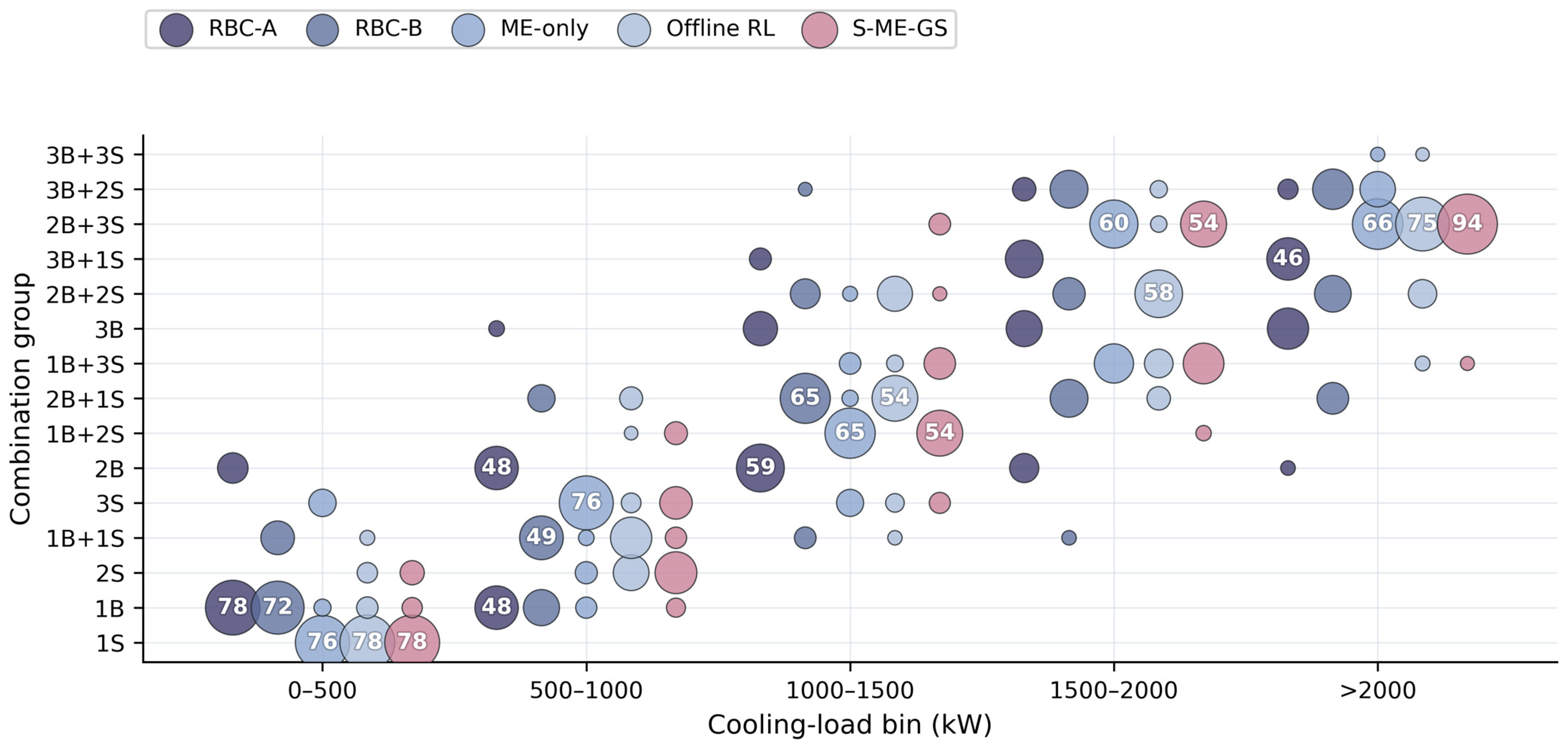
The aggregate electricity totals do not fully reveal how each strategy uses the available combination-group space. Figure 15 therefore projects the operating record onto the combination-group and cooling-load-bin plane. RBC-A and RBC-B show sequence-oriented utilization patterns, with operating time concentrated on a limited set of groups determined by their fixed staging sequences. ME-only and Offline RL visit a wider range of groups, but several load bins are still dominated by a small number of preferred combinations.

S-ME-GS exhibits a more adaptive utilization pattern. In low- and medium-load regions, it distributes operation across neighboring combination groups instead of relying on a single dominant group or a fixed staging path. At higher loads, it naturally shifts toward higher-capacity groups as the capacity constraint becomes more restrictive. These results suggest that the energy savings of S-ME-GS are supported by a more flexible use of heterogeneous unit combinations across the operating range.

4.2.2. Unit PLR Distribution

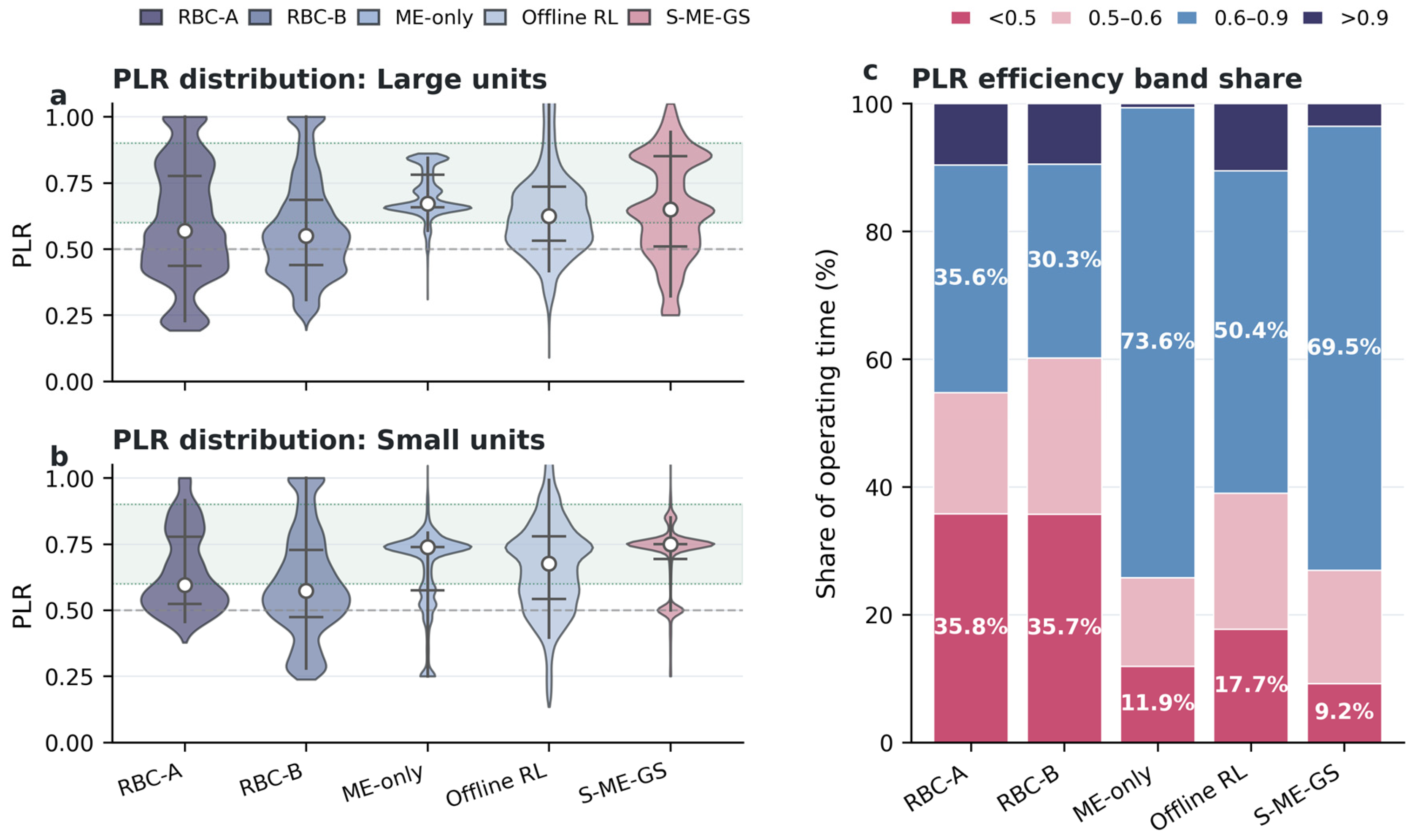
The energy differences are reflected at the unit level by the PLR distributions in Figure 16. For large units, RBC-A and RBC-B show broad distributions ranging from low to high PLR levels, with medians around the middle of the operating range. This indicates that the fixed staging sequences retain redundant online capacity during part–load hours. Offline RL narrows the distribution toward the medium-PLR range, but a low-PLR tail remains. ME-only and S-ME-GS both shift large-unit operation toward higher PLR levels, with S-ME-GS concentrating more operating time near the upper part of the 0.6–0.9 high-efficiency range.

For small units, the differences among strategies are also evident. The RBC strategies operate small units over a wide PLR range, with substantial time spent at both medium and high fractional loads. This reflects the limited flexibility of fixed allocation rules when the active combination has already been determined. ME-only concentrates small-unit operation more strongly within the high-efficiency band, while Offline RL retains a broader spread. S-ME-GS avoids excessive low-PLR operation and keeps most small-unit operation within the medium-to-high PLR range, indicating that the selected combinations and flow allocations better match the part–load operating conditions.

The efficiency-band shares in Figure 16c provide a compact summary of these distributional differences. RBC-A and RBC-B leave 35.8% and 35.7% of operating time below 0.5 PLR, respectively, indicating persistent over-staging. ME-only achieves the highest high-efficiency-band share, at 73.6%, but still has 11.9% of operating time below 0.5 PLR. S-ME-GS achieves the lowest low-PLR share, at 9.2%, while maintaining a high-efficiency-band share of 69.5%. Although this high-efficiency-band share is lower than that of ME-only, S-ME-GS substantially reduces low-PLR operation, showing that its energy performance is supported by both improved loading quality and path-level coordination.

4.2.3. Unit Switching Stability

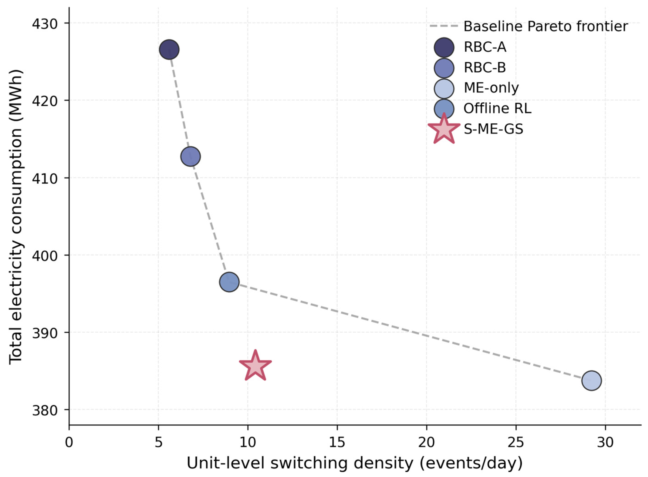
As shown in Figure 17, the four baselines fall along a clear Pareto frontier in which lower electricity consumption is consistently traded against higher switching density. RBC-A and RBC-B occupy the upper-left region with the lowest switching densities, at 5.6 and 6.8 events per day, but also show the highest electricity consumption. ME-only sits at the opposite extreme, with 29.2 events per day and the lowest electricity consumption. This reflects the tendency of current-step marginal-efficiency optimization to repeatedly adjust the active unit set near low-power combination boundaries. Offline RL moves toward the interior of the trade-off space, with a switching density of 9.0 events per day, indicating that action regularization suppresses frequent reversals but does not achieve the same energy level as ME-only.

S-ME-GS is positioned below the baseline frontier. It operates at 10.5 events per day with 654 unit-level switches. Its switching density is comparable to that of Offline RL and modestly above the RBC baselines, while its energy consumption remains within 0.50% of the ME-only reference case. No baseline combination of energy consumption and switching density dominates S-ME-GS along either axis.

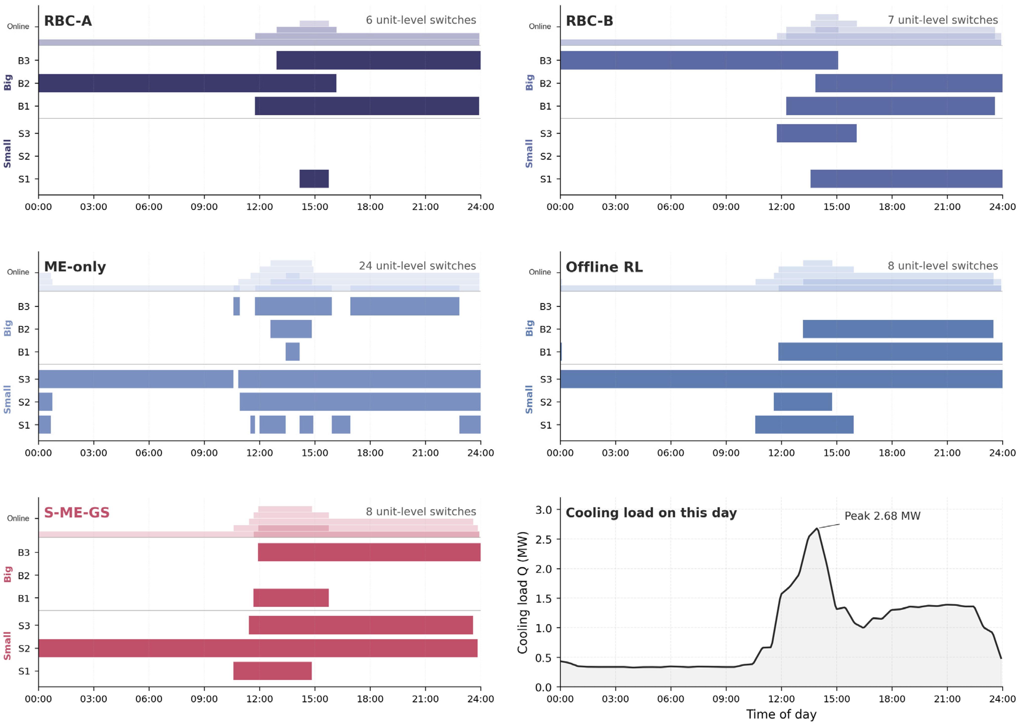
Figure 18 shows the per-unit schedules on a representative day with strong load variations. The four baselines exhibit qualitatively distinct patterns. RBC-A keeps one large unit online overnight, adds additional large-unit capacity during the afternoon ramp-up, and then retains two large units until midnight, resulting in over-commitment during and after the peak. RBC-B rearranges the same logic into a different large-unit sequence but inherits a similar overnight or late-day over-commitment tendency. ME-only generates 24 unit-level transitions concentrated in the 10:30–18:00 window. The active large unit changes three times in the afternoon, and one of the small units is repeatedly switched on and off within four hours. Offline RL produces eight transitions overall but commits two large units and one small unit together from afternoon until midnight, repeating the over-commitment pattern of RBC, with fewer transitions.

S-ME-GS produces the same eight transitions as Offline RL but arranges them differently. It maintains one small unit overnight, adds large-unit and small-unit capacity around the late-morning load transition, releases one large unit and one small unit once the load begins to fall, and keeps a one-large and two-small configuration for the evening period. All transitions are concentrated near the dominant load turning points, leaving the active combination stable throughout both the peak hours and the overnight period. The schedule is responsive at the transitions and stable between them.

4.2.4. Thermal Reliability Under Load Variations

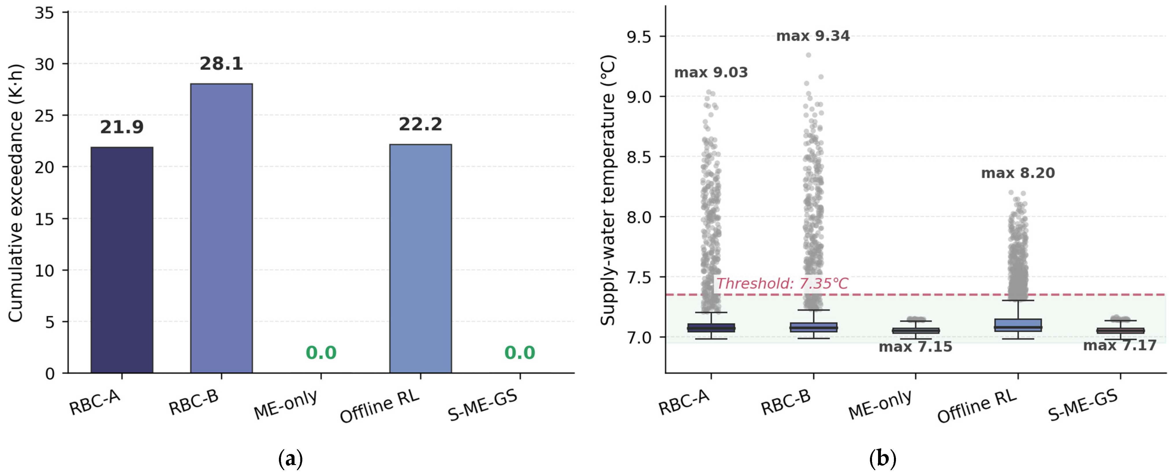
Thermal reliability separates the strategies into three qualitatively distinct violation patterns rather than a single ranking. The cumulative violation measured as K·h above the 7.35 °C threshold is shown in Figure 19a. Both RBC variants accumulate substantial violation totals of 21.9 and 28.1 K·h, comparable to or exceeding that of Offline RL at 22.2 K·h, while ME-only and S-ME-GS register zero. The RBC strategies, despite their conservative switching, do not deliver the best thermal reliability.

The mechanism behind the three patterns becomes clear from the temperature distribution during rapid load-rise periods in Figure 19b, defined as control steps where $dQ/dt$ exceeds 200 kW/h. RBC-A and RBC-B exhibit numerous outlier samples extending to 9.03 °C and 9.34 °C respectively, well above the threshold band. These are short and frequent spikes. The feedback-threshold logic requires the supply-water temperature, PLR, or load to remain above a trigger for a minimum duration before adding capacity, so the system continues with the existing combination during the early control steps of a steep ramp. The deviation is large in magnitude but resolves within a few control steps once the threshold logic responds. Offline RL shows a different pattern with fewer extreme outliers, with a maximum of 8.20 °C, but a wider interquartile range around the threshold line, corresponding to longer-duration excursions. This is consistent with a policy whose training objective emphasizes energy and switching but does not explicitly encode high-percentile capacity risk. The learned policy therefore operates online units close to the upper edge of their PLR range and leaves limited reserve for instantaneous disturbances.

ME-only and S-ME-GS both remain below the threshold, with maxima of 7.15 °C and 7.17 °C. ME-only can avoid thermal violation because its current-step marginal-efficiency search reselects a feasible active-unit combination whenever the measured load approaches the capacity or PLR boundary. This makes the controller highly responsive to rapid load changes, but the same mechanism also causes frequent active-set changes, as reflected by its 29.2 switching events per day. S-ME-GS retains the feasibility screening and marginal-efficiency allocation of this mechanism, but adds finite-horizon reserve evaluation and transition-cost terms. As a result, it preserves zero exceedance while reducing switching to 10.5 events per day, indicating that its main advantage over ME-only is not stronger instantaneous feasibility, but better path-level judgment of whether a staging action is worth executing.

4.3. Mechanism Analysis

The preceding evaluation shows that S-ME-GS achieves the most balanced overall performance among the compared strategies. It reduces plant electricity consumption while maintaining a healthy online-capacity utilization level, suppressing unnecessary switching actions, and avoiding cumulative supply-temperature violations. This result indicates that the proposed method does not improve one objective at the direct expense of another. Instead, it coordinates energy efficiency, operational stability, and thermal reliability through the joint action of graph-based combination search, marginal-efficiency allocation, and scenario-aware activation gating.

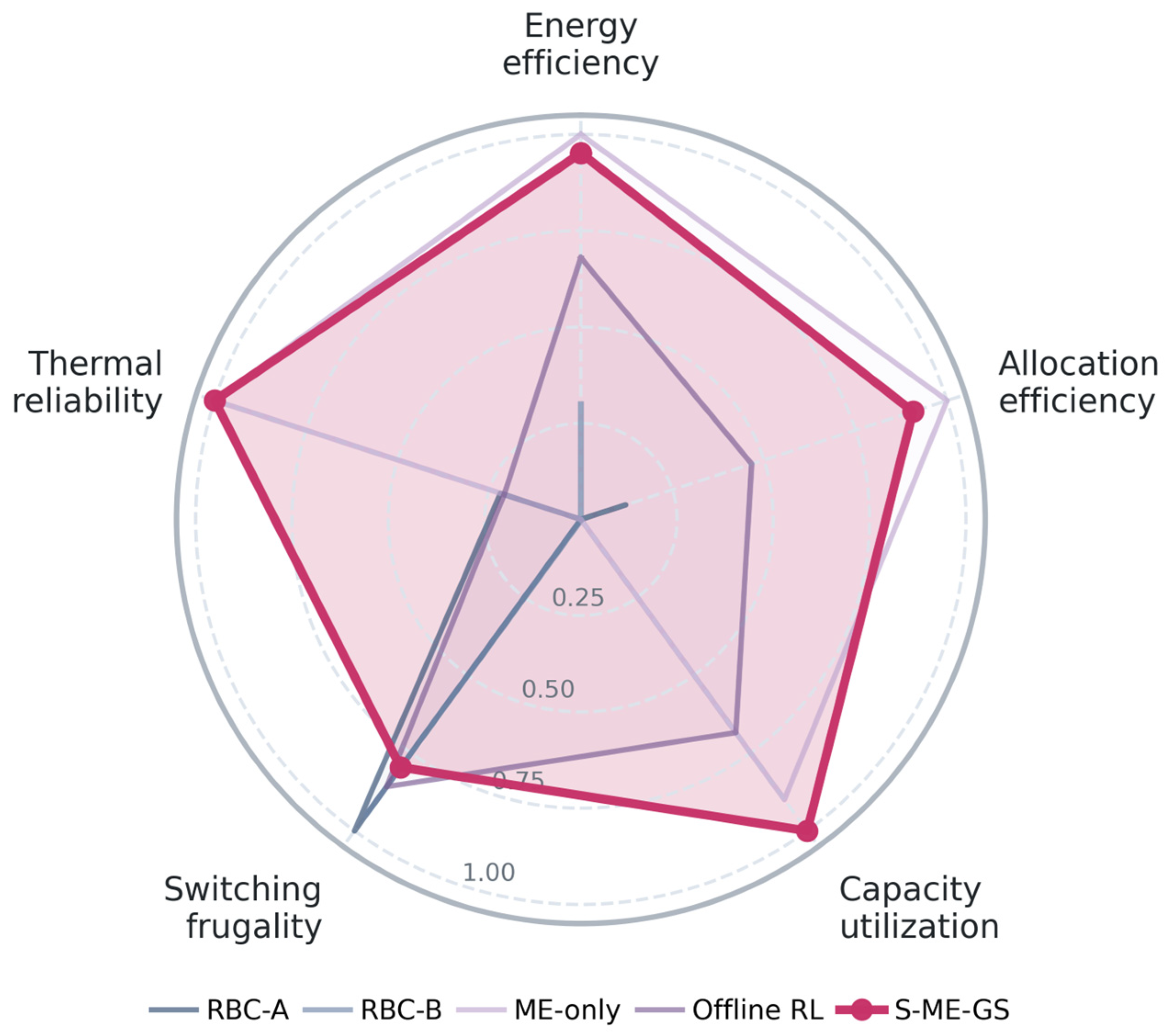
Figure 20 summarizes this overall balance using normalized performance scores. ME-only exhibits strong energy performance, but its action smoothness and switching stability are weakened by frequent responses to local efficiency changes. The rule-based baselines maintain relatively stable switching behavior, but their fixed staging sequences limit both PLR quality and thermal reliability. Offline RL improves some aspects of operation but still shows an uneven profile across the evaluated dimensions. In contrast, S-ME-GS maintains high scores across all five axes, forming a more rounded radar shape. This indicates that its advantage is not a single-metric optimum, but a more balanced operating profile across the main control objectives.

The comparison between ME-only and S-ME-GS also provides a partial ablation of the proposed decision structure. ME-only retains current-step marginal-efficiency allocation and feasibility screening, whereas S-ME-GS adds finite-horizon graph search, reserve-risk evaluation, transition penalties, and the activation-margin gate. The reduction in switching with only a small energy increase therefore reflects the contribution of the path-level decision layer rather than the forecasting module alone.

This balance can be explained by the three structural components of the proposed method. First, the graph search relaxes the sequence-bound limitation of conventional rule-based control. Instead of following a predefined large-first or alternating staging order, S-ME-GS evaluates feasible unit combinations over a finite horizon. The selected trajectory therefore depends on both the current load and the expected near-future load evolution. This allows the controller to move toward load-matched combinations that provide sufficient capacity without retaining excessive online units.

Second, the marginal-efficiency allocator improves the within-combination load distribution. In heterogeneous plants, equal-load or capacity-proportional allocation cannot fully reflect the different part–load characteristics of large and small units. As a result, some units may be pushed away from their efficient PLR regions even when the selected combination appears reasonable at the plant level. The marginal-efficiency allocator addresses this issue by distributing the cooling demand according to the joint efficiency surface of the active units. Therefore, the plant can maintain favorable utilization without relying on a fixed dispatch table.

Third, the scenario-aware activation margin controls whether a candidate transition should actually be executed. This mechanism is essential because opening the combination space and optimizing dispatch alone may still lead to frequent reversals near combination boundaries. A transition is admitted only when its predicted path-cost improvement exceeds the active margin. Since the margin changes with the operating scenario, the controller can be more conservative during rising-load and high-load periods, while allowing safer capacity release during falling-load periods. In this way, the method avoids both excessive switching and delayed response.

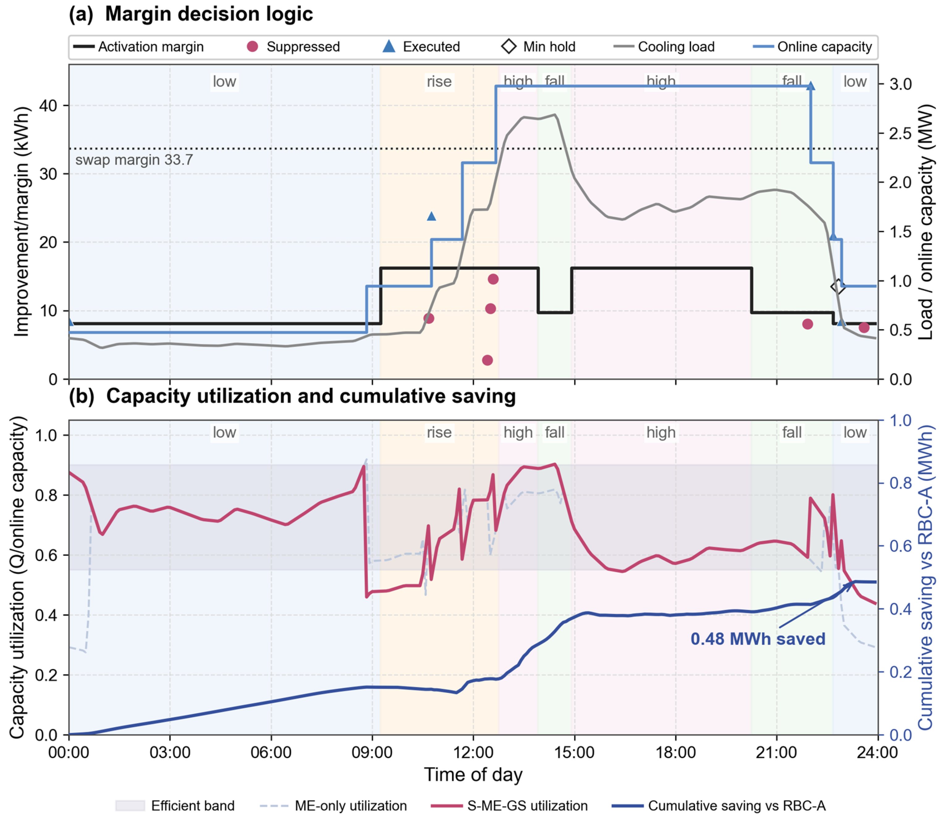
Figure 21 illustrates this mechanism on a representative day. In Figure 21a, the activation margin varies with the identified operating scenario. Suppressed candidates are mostly located below the active margin, whereas executed actions occur only when the expected path-cost improvement is sufficiently large. The higher swap threshold further prevents paired start–stop transitions unless the predicted benefit clearly justifies the action. This behavior shows that S-ME-GS does not simply choose the lowest-power combination at each step. Instead, it filters candidate transitions according to their expected persistence and operational consequence.

The physical effect of this decision logic is shown in Figure 21b. Compared with the ME-only reference, S-ME-GS keeps the online-capacity utilization within the efficient band for a larger portion of the day and avoids sharp utilization fluctuations around scenario boundaries. The cumulative saving curve relative to RBC-A increases steadily, indicating that the retained reserve capacity does not lead to a later energy penalty. Meanwhile, the representative-day statistics show fewer switches, smoother unit schedules, and no extreme utilization events. These results suggest that the activation margin suppresses low-value actions while preserving the energy benefit of graph-based optimization.

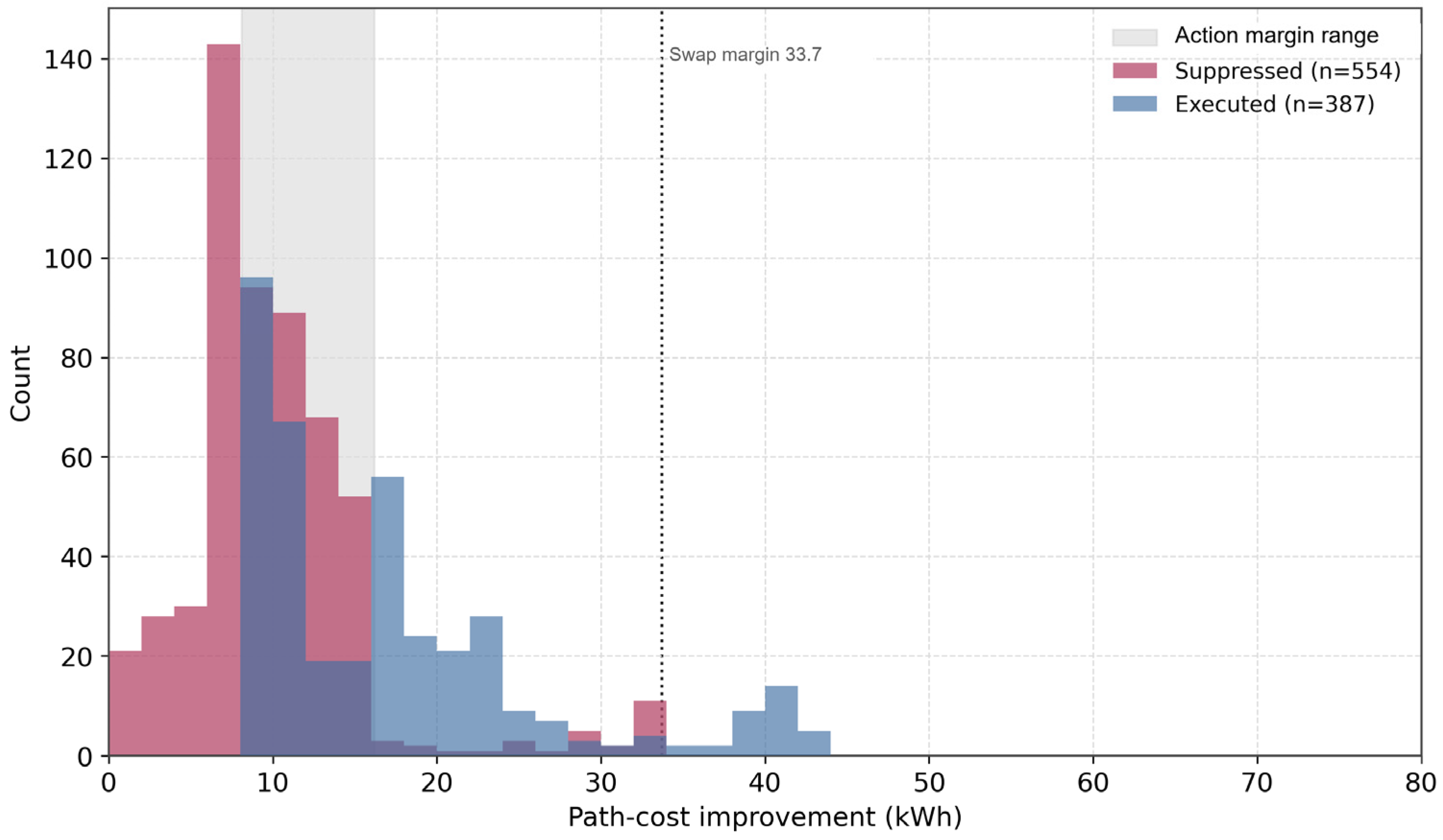
Figure 22 further verifies that this behavior is not limited to the selected representative day. Across the full evaluation period, suppressed candidates are concentrated below the calibrated action-margin range, while executed candidates extend toward higher path-cost improvements. The overlap near the margin is expected because the admissibility threshold is scenario-dependent rather than fixed. This distribution confirms that the activation gate separates marginal, easily reversible actions from transitions with stronger predicted benefits.

Overall, the three components of S-ME-GS play complementary roles. Graph search expands the reachable combination space, marginal-efficiency allocation improves within-combination dispatch, and the scenario-aware margin filters low-value transitions. Their joint effect explains why S-ME-GS achieves a balanced trade-off among electricity consumption, PLR quality, switching stability, and thermal reliability.

4.4. Practical Implications and Limitations

The proposed method provides a plant-level supervisory decision framework for coordinating active-unit selection and load allocation in heterogeneous cooling plants. By formulating the problem in terms of feasible unit combinations, marginal-efficiency allocation, reserve adequacy, and transition costs, S-ME-GS keeps the main decision factors explicit and inspectable. This structure is useful for engineering applications, in which energy efficiency, switching stability, and supply-temperature reliability must be balanced under discrete equipment constraints.

The results indicate that the supervisory decision problem can be evaluated with a lightweight online planner. The layered dynamic-programming implementation constructs candidate paths from the current operating state, expands only feasible neighboring transitions, and retains a limited set of low-cost paths. The benchmark in Appendix A shows that the planner requires less than 0.1% of the 5-min control interval in the tested configuration. This supports the computational tractability of the method and indicates that graph search over unit combinations can be feasible for real-time supervisory control.

The framework is structurally transferable because active-unit combinations, load-allocation efficiency, reserve adequacy, and transition penalties are common elements in heterogeneous multi-unit cooling plants. However, the numerical parameterization is plant-specific. Applying the method to another plant would require re-identification of equipment performance curves, capacity limits, hydraulic constraints, reserve ratios, transition penalties, and scenario-dependent weights according to the target system and operating policy.

Several limitations should also be noted. First, the closed-loop validation is based on one heterogeneous air-source heat-pump plant in a TRNSYS-Python co-simulation environment. Although the method is not tied to this specific plant layout, broader validation is needed before claiming general performance across different cooling-plant configurations. Second, forecast quality affects reserve evaluation and action activation. The residual-quantile envelope partially protects the planner from point-forecast error, but unusual weather, occupancy, or operational events may still require conservative operator-defined limits. Third, the present study reports reproducible implementation evidence, including calibrated supervisory weights, planner runtime, and forecasting error, but does not provide a full cross-plant sensitivity analysis. The residual-quantile envelope is an empirical uncertainty representation and does not constitute a full stochastic optimization over all possible future load paths. The data set also does not include multiple weather years or alternative climate profiles, so the reported improvements should be interpreted as evidence for the tested plant and operating record rather than as a statistical guarantee across climates. Therefore, S-ME-GS should be viewed as a transferable supervisory-control framework that requires plant-specific calibration rather than as a fixed parameter set.

5. Conclusions

This study proposed S-ME-GS, a scenario-driven marginal-efficiency graph-search method for supervisory control of heterogeneous multi-unit cooling plants. By integrating short-term load representation, residual-quantile uncertainty bands, marginal-efficiency load allocation, and layered finite-horizon graph search, the method provides an interpretable decision framework for coordinating active-unit selection, load distribution, reserve adequacy, and transition costs. This formulation addresses key limitations of conventional supervisory control, including fixed staging sequences, redundant low-PLR operation, and myopic switching under load fluctuations.

The 62-day TRNSYS-Python closed-loop co-simulation demonstrates that S-ME-GS improves the main trade-off that conventional supervisory strategies struggle to balance. Compared with the two rule-based controls, S-ME-GS reduced electricity consumption by 9.61% and 6.59%, respectively, while avoiding the restricted combination usage and redundant online capacity caused by fixed staging sequences. Compared with the ME-only current-step energy reference, S-ME-GS kept energy consumption within 0.50% but reduced switching density from 29.2 to 10.5 events per day, showing that path-level evaluation suppresses myopic switching without sacrificing most of the energy benefit. In addition, S-ME-GS maintained zero supply-temperature exceedance, whereas the RBC strategies and Offline RL showed temperature violations under rapid load variations.

The layered graph-search implementation solved each control step in 85.3 ms on average and 227.5 ms at maximum, well below the 5-min supervisory interval. These results indicate that S-ME-GS provides a computationally tractable and interpretable supervisory-control framework for balancing energy efficiency, switching stability, and supply-temperature reliability in heterogeneous cooling plants. Future work will focus on adaptive seasonal recalibration, field-trial validation, and extension to larger cooling plants with more diverse equipment configurations and operating constraints.