Author Contributions
Conceptualization, M.P., J.H., S.M., V.P. and Z.H.; methodology, M.P., J.H., S.M. and Z.H.; software, K.M., L.F., J.H. and S.M.; validation, M.P., S.M., V.P. and Z.H.; formal analysis, F.H., K.M., L.F. and J.H.; investigation, F.H.; resources, F.H. and M.P.; data curation, F.H.; writing—original draft preparation, K.M. and L.F.; writing—review and editing, K.M., M.P., Z.H., S.M., J.H., L.F., F.H. and V.P.; visualization, K.M., J.H., L.F. and S.M.; supervision, M.P.; project administration, M.P.; funding acquisition, M.P. All authors have read and agreed to the published version of the manuscript.
Figure 1.
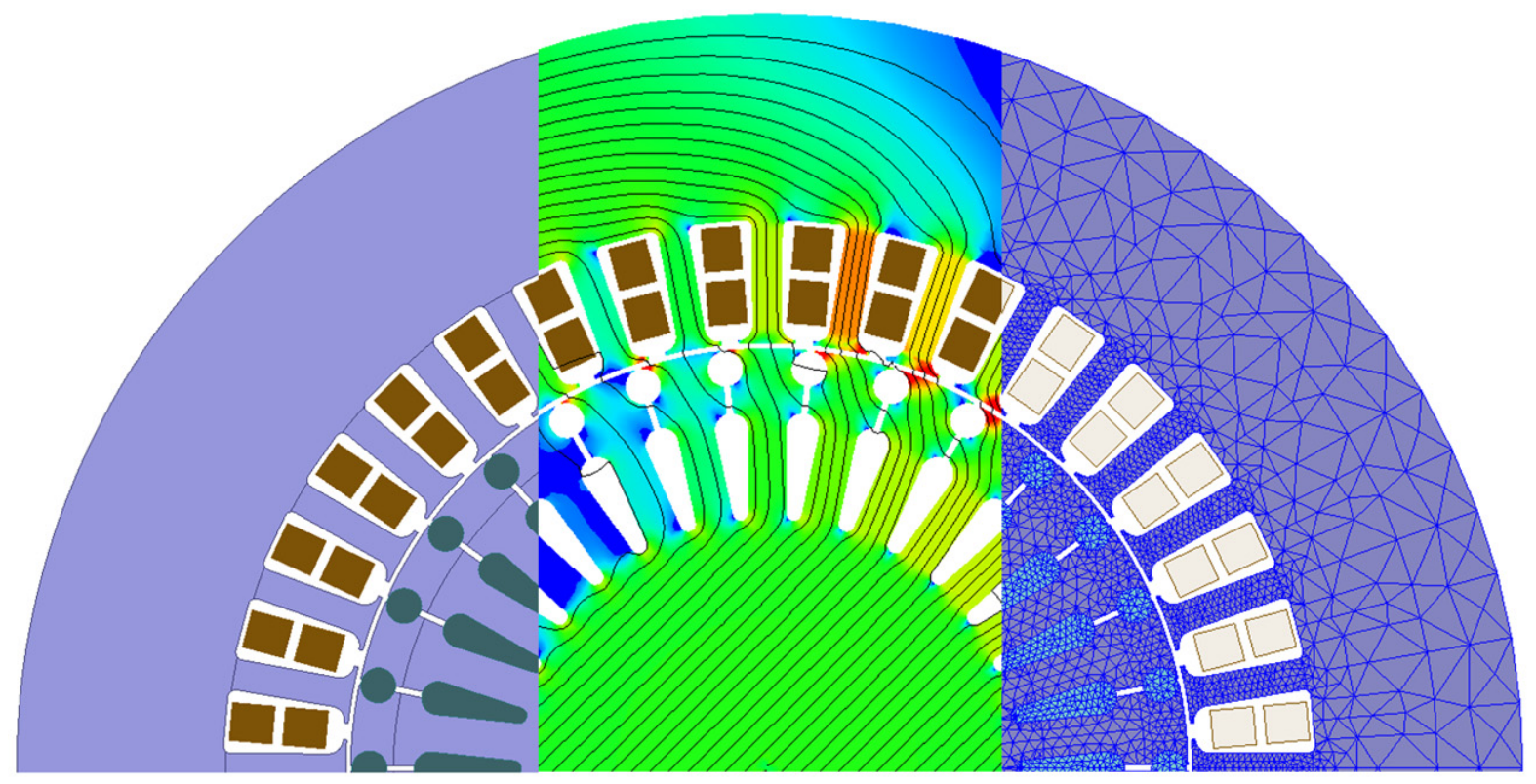
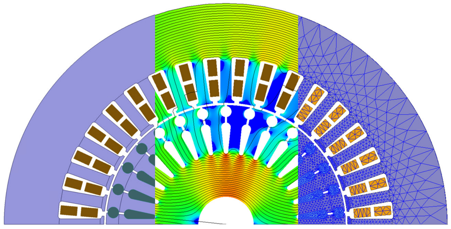
Electromagnetic FEM model of the machine: mesh and magnetic flux density at the nominal load point (100 kW at 13,000 rpm). The left portion of the figure displays the stator and rotor (blue), the armature winding (brown) and the rotor bars (dark green). The middle portion illustrates the flux density distribution, where blue indicates low flux density and red indicates high flux density.
Figure 1.
Electromagnetic FEM model of the machine: mesh and magnetic flux density at the nominal load point (100 kW at 13,000 rpm). The left portion of the figure displays the stator and rotor (blue), the armature winding (brown) and the rotor bars (dark green). The middle portion illustrates the flux density distribution, where blue indicates low flux density and red indicates high flux density.
Figure 2.
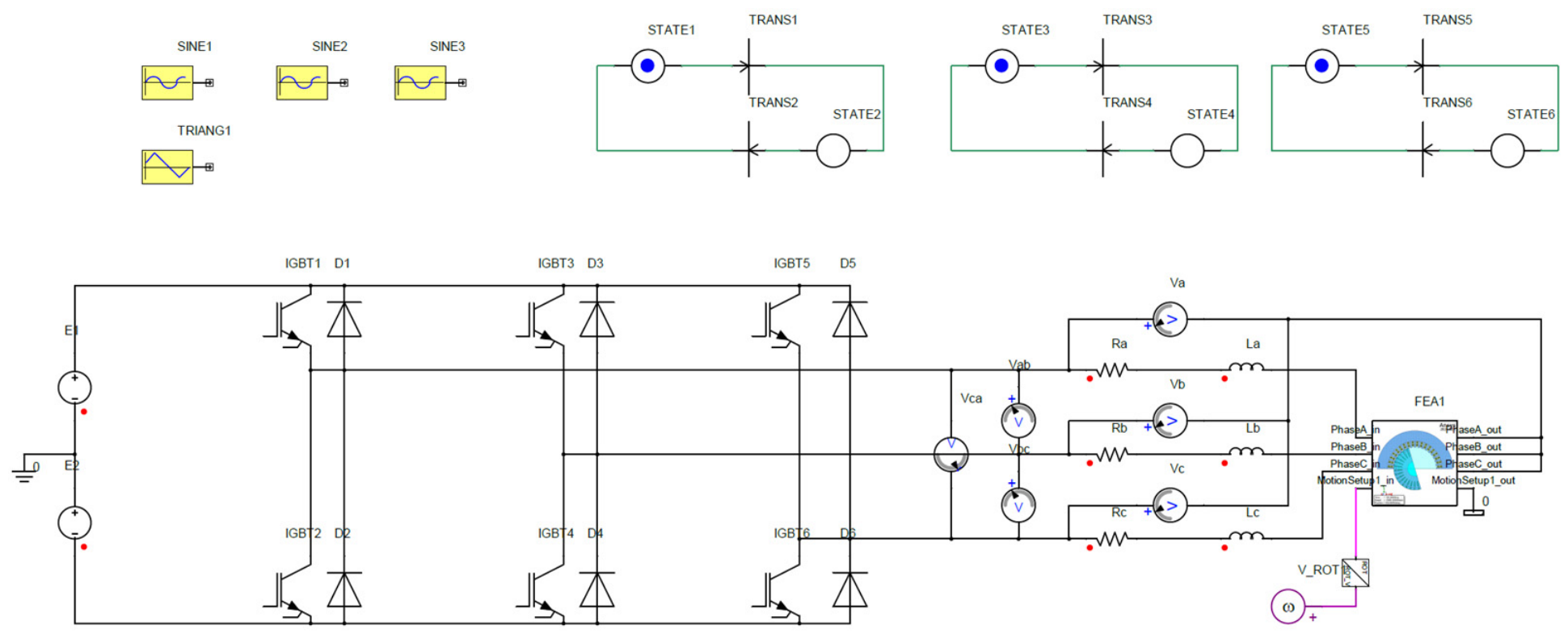
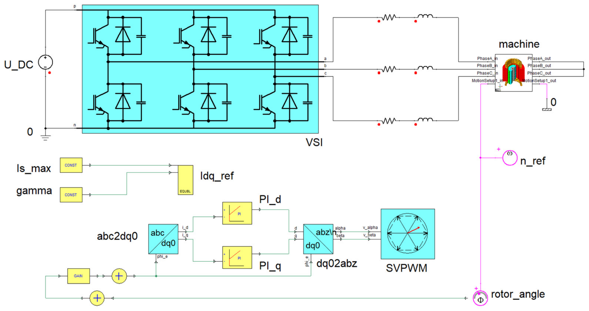
Model of the power converter coupled with an electric machine model.
Figure 2.
Model of the power converter coupled with an electric machine model.
Figure 3.
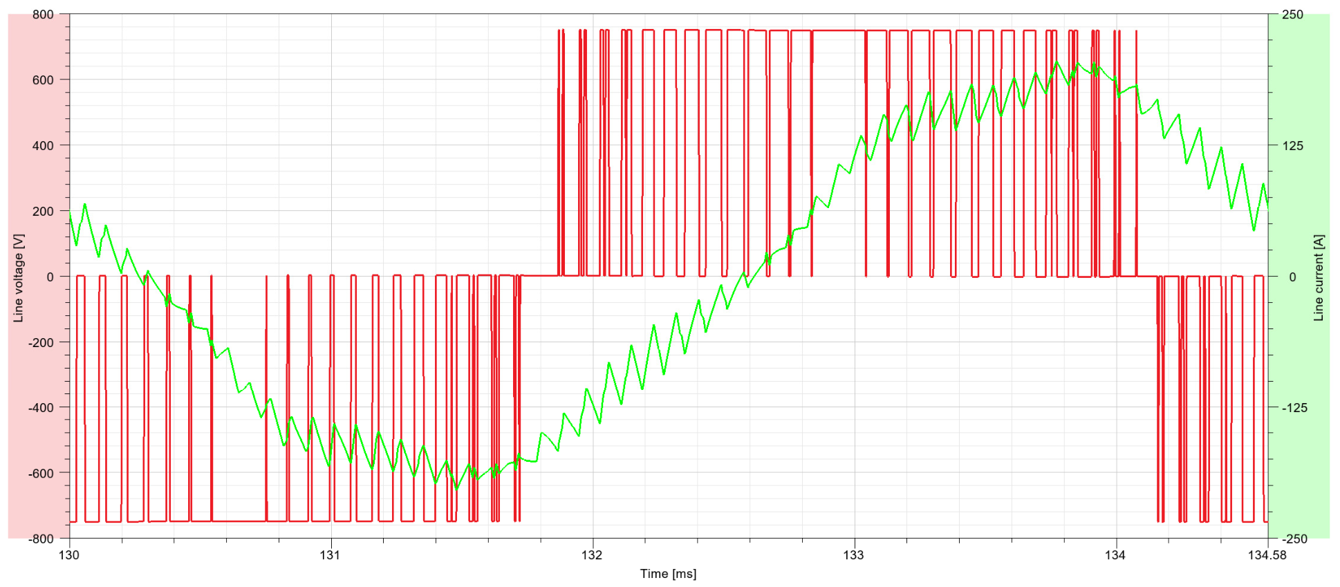
Simulated line voltage and the corresponding armature winding current.
Figure 3.
Simulated line voltage and the corresponding armature winding current.
Figure 4.
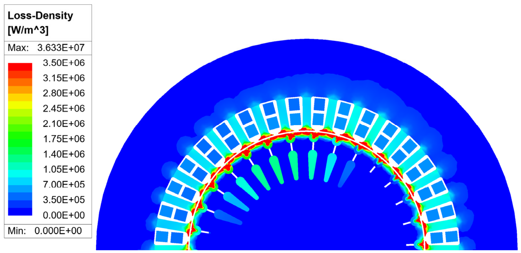
Calculated loss density results at 13,000 rpm under full-load operation.
Figure 4.
Calculated loss density results at 13,000 rpm under full-load operation.
Figure 5.
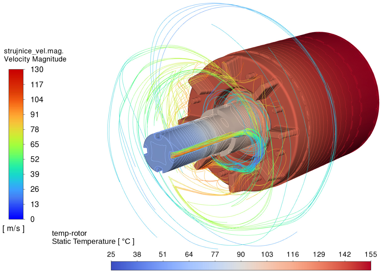
Temperature field of the rotor with streamlines through shaft channels and in the end region.
Figure 5.
Temperature field of the rotor with streamlines through shaft channels and in the end region.
Figure 6.
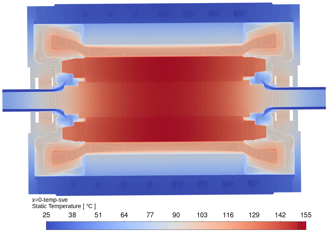
Temperature contours resulting from a steady-state 3D CHT model of the lower-speed prototype.
Figure 6.
Temperature contours resulting from a steady-state 3D CHT model of the lower-speed prototype.
Figure 7.
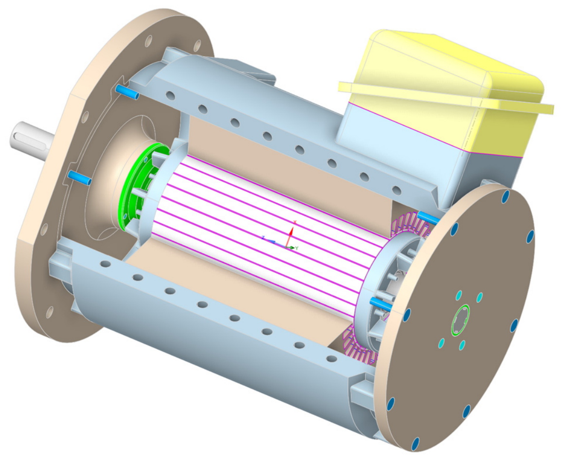
CAD model used for mechanical analyses. The figure shows the following components: housing (light blue), end shields (brown), stator core (brown), laminated rotor (white with magenta outlines), bearing covers (green) and fastening elements (blue).
Figure 7.
CAD model used for mechanical analyses. The figure shows the following components: housing (light blue), end shields (brown), stator core (brown), laminated rotor (white with magenta outlines), bearing covers (green) and fastening elements (blue).
Figure 8.
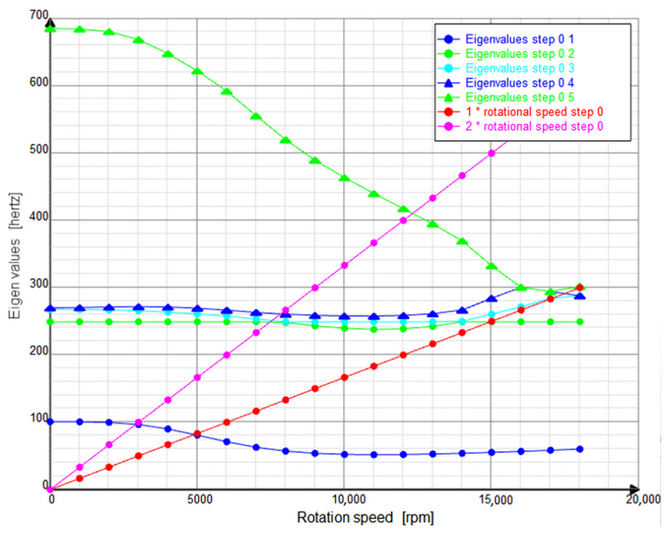
Critical speed map of lower-speed prototype rotor. The colors are as follows: the axial vibration mode at 57 Hz (blue), the first bending vibration mode at 248 Hz (green), the first-order electromagnetic excitation (inclined red), the second-order electromagnetic excitation (inclined pink).
Figure 8.
Critical speed map of lower-speed prototype rotor. The colors are as follows: the axial vibration mode at 57 Hz (blue), the first bending vibration mode at 248 Hz (green), the first-order electromagnetic excitation (inclined red), the second-order electromagnetic excitation (inclined pink).
Figure 9.
Model of the induction machine used in simulations, along with the mesh and the magnetic flux density distribution at the nominal load point (60 kW at 15,000 rpm). The left portion of the figure displays the stator and rotor (blue), the armature winding (brown), and the rotor bars (dark green). The middle portion illustrates the flux density distribution, where blue indicates low flux density and red indicates high flux density.
Figure 9.
Model of the induction machine used in simulations, along with the mesh and the magnetic flux density distribution at the nominal load point (60 kW at 15,000 rpm). The left portion of the figure displays the stator and rotor (blue), the armature winding (brown), and the rotor bars (dark green). The middle portion illustrates the flux density distribution, where blue indicates low flux density and red indicates high flux density.
Figure 10.
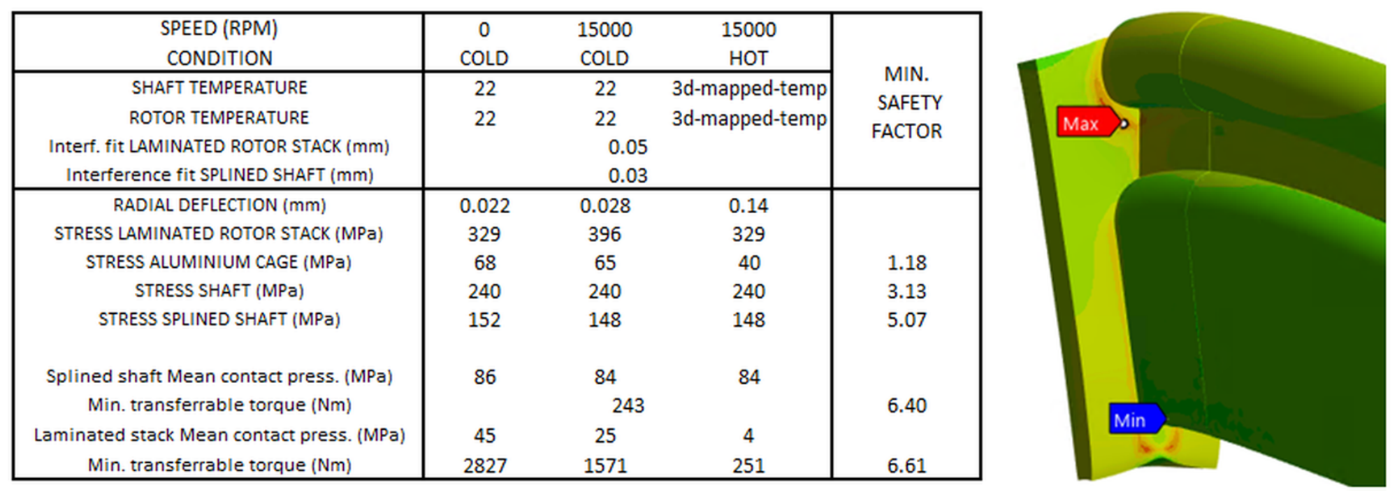
Overview of contact-loss safety and strength safety factors of main structural components.
Figure 10.
Overview of contact-loss safety and strength safety factors of main structural components.
Figure 11.
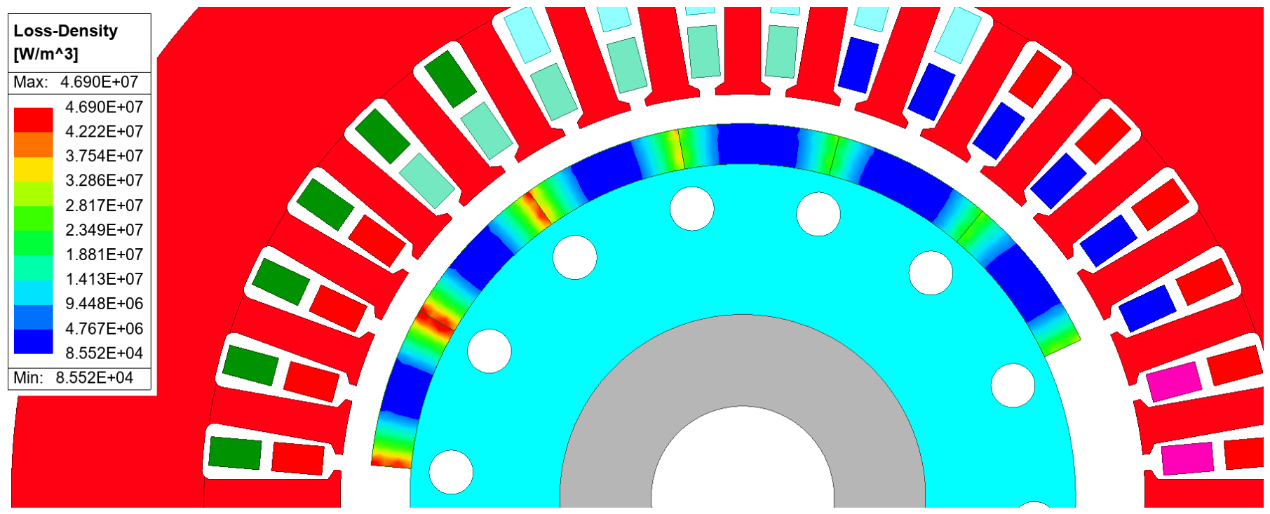
Loss density in permanent magnets at a nominal working point (100 kW at 25,000 rpm).
Figure 11.
Loss density in permanent magnets at a nominal working point (100 kW at 25,000 rpm).
Figure 12.
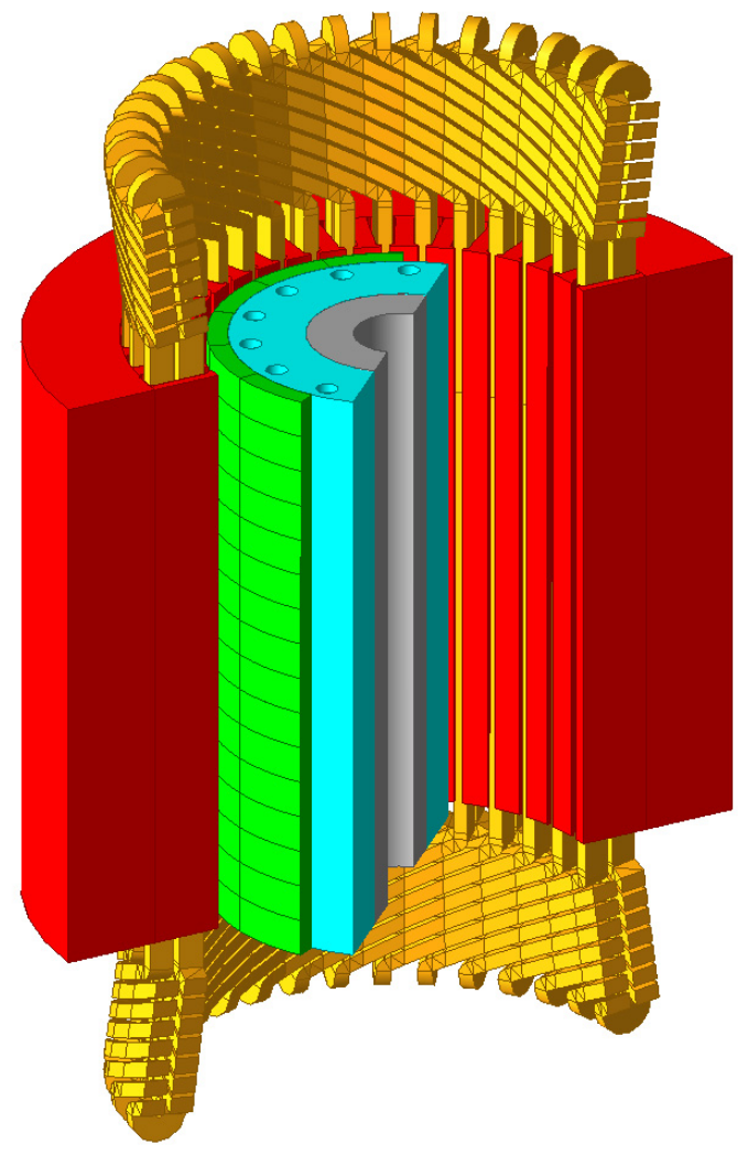
Split 3D machine model used in FEM simulations. The stator is shown in red, rotor in blue, shaft in grey, permanent magnets in green, and armature winding in orange.
Figure 12.
Split 3D machine model used in FEM simulations. The stator is shown in red, rotor in blue, shaft in grey, permanent magnets in green, and armature winding in orange.
Figure 13.
Coupled simulation of the 3D FEM machine model and the power converter.
Figure 13.
Coupled simulation of the 3D FEM machine model and the power converter.
Figure 14.
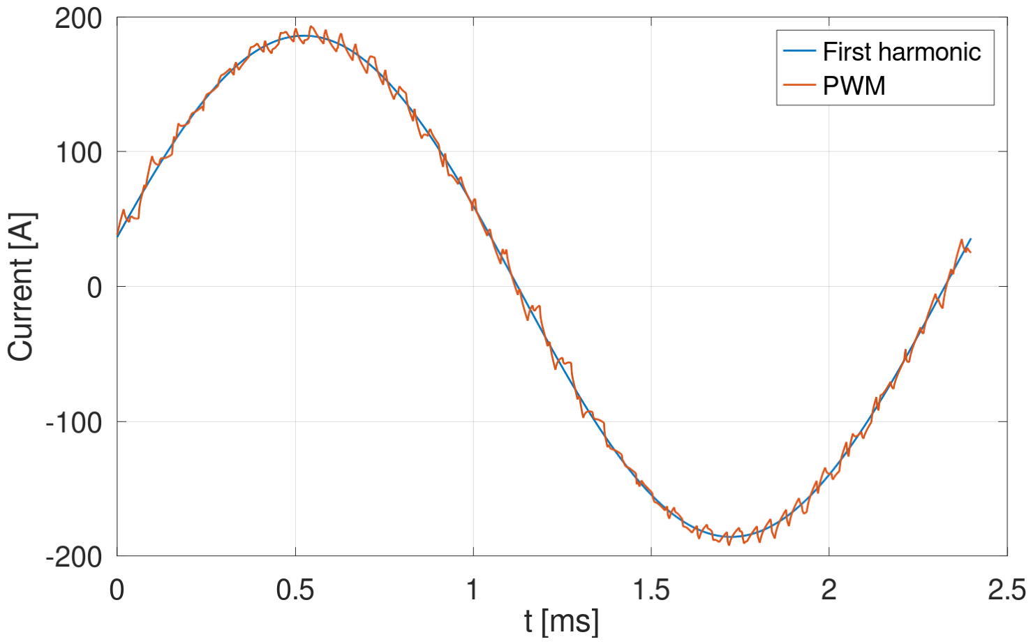
PWM current waveform and the corresponding first harmonic.
Figure 14.
PWM current waveform and the corresponding first harmonic.
Figure 15.
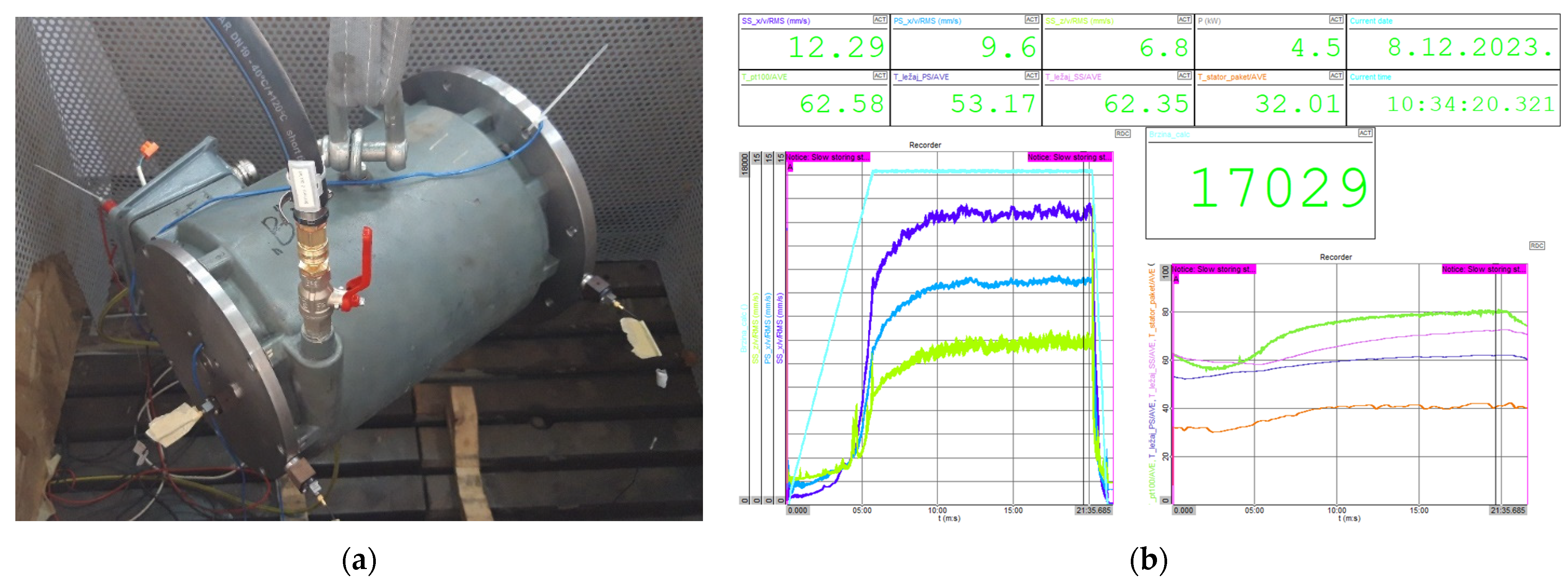
No load testing of the machine: (a) machine; (b) measurements. The left graph displays the operating speed (light blue), the radial component of vibrations at the NDE (violet) and DE (blue), and the axial component of vibrations at the NDE (green). The right graph illustrates the winding temperature (green), the bearing temperatures at the NDE (pink) and DE (dark blue), and the stator outer diameter temperature (orange).
Figure 15.
No load testing of the machine: (a) machine; (b) measurements. The left graph displays the operating speed (light blue), the radial component of vibrations at the NDE (violet) and DE (blue), and the axial component of vibrations at the NDE (green). The right graph illustrates the winding temperature (green), the bearing temperatures at the NDE (pink) and DE (dark blue), and the stator outer diameter temperature (orange).
Figure 16.
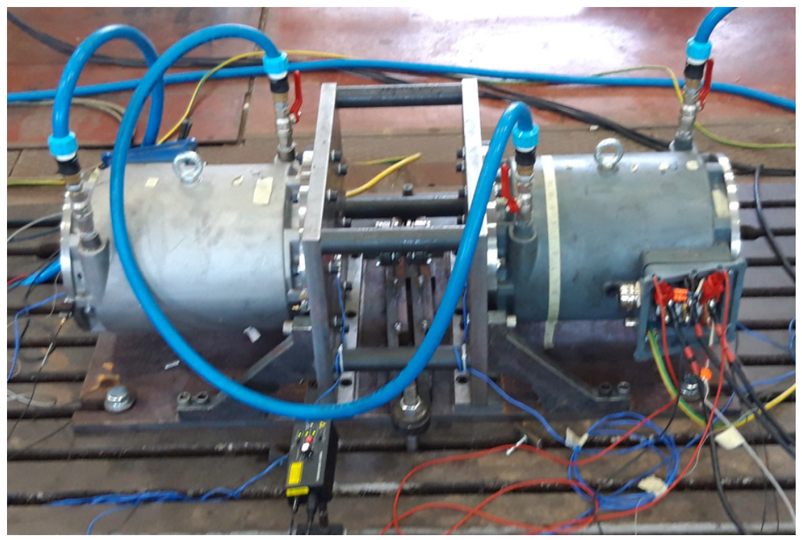
Back-to-back testing setup for machine load tests.
Figure 16.
Back-to-back testing setup for machine load tests.
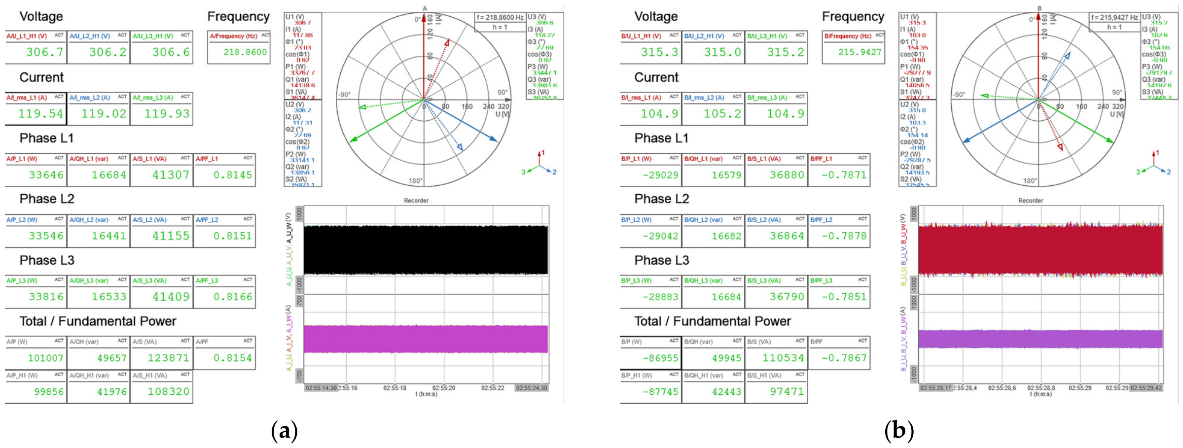
Figure 17.
Measurements for the rated load condition: (a) motor machine; (b) generator machine. Phase-specific and cumulative operational data for motor and generator machines. The phasor diagrams illustrate the voltage (solid arrows) and current (dashed arrows) vectors for phase 1 (red), phase 2 (blue), and phase 3 (green). The time-domain graphs displayed below the phasor diagrams contain the corresponding waveforms (note that individual cycles are not visible due to the large time-window scale).
Figure 17.
Measurements for the rated load condition: (a) motor machine; (b) generator machine. Phase-specific and cumulative operational data for motor and generator machines. The phasor diagrams illustrate the voltage (solid arrows) and current (dashed arrows) vectors for phase 1 (red), phase 2 (blue), and phase 3 (green). The time-domain graphs displayed below the phasor diagrams contain the corresponding waveforms (note that individual cycles are not visible due to the large time-window scale).
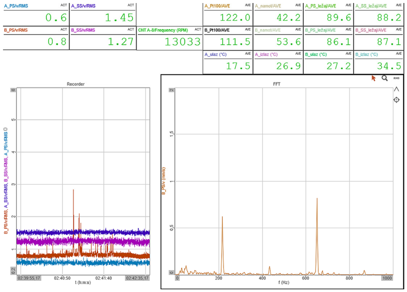
Figure 18.
Measured temperature and vibrations for the rated load condition. The left graph displays the waveforms of the vibrations at the DE and NDE for both the motor (turquoise and violet, respectively) and the generator (orange and magenta, respectively). The right graph shows the FFT analysis of the generator vibrations at the DE.
Figure 18.
Measured temperature and vibrations for the rated load condition. The left graph displays the waveforms of the vibrations at the DE and NDE for both the motor (turquoise and violet, respectively) and the generator (orange and magenta, respectively). The right graph shows the FFT analysis of the generator vibrations at the DE.
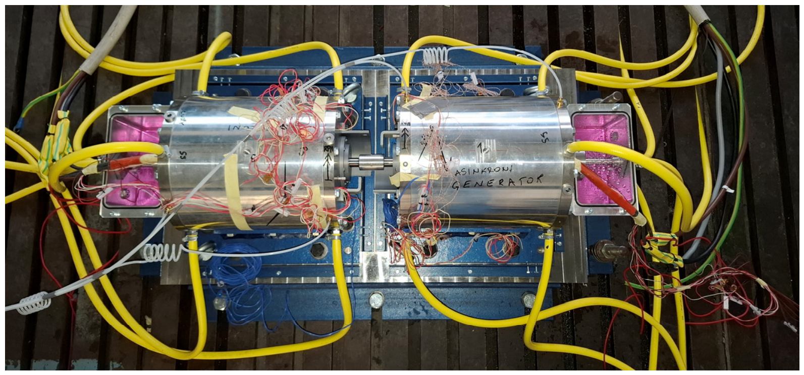
Figure 19.
Back-to-back testing setup for high-speed machine prototypes from above.
Figure 19.
Back-to-back testing setup for high-speed machine prototypes from above.
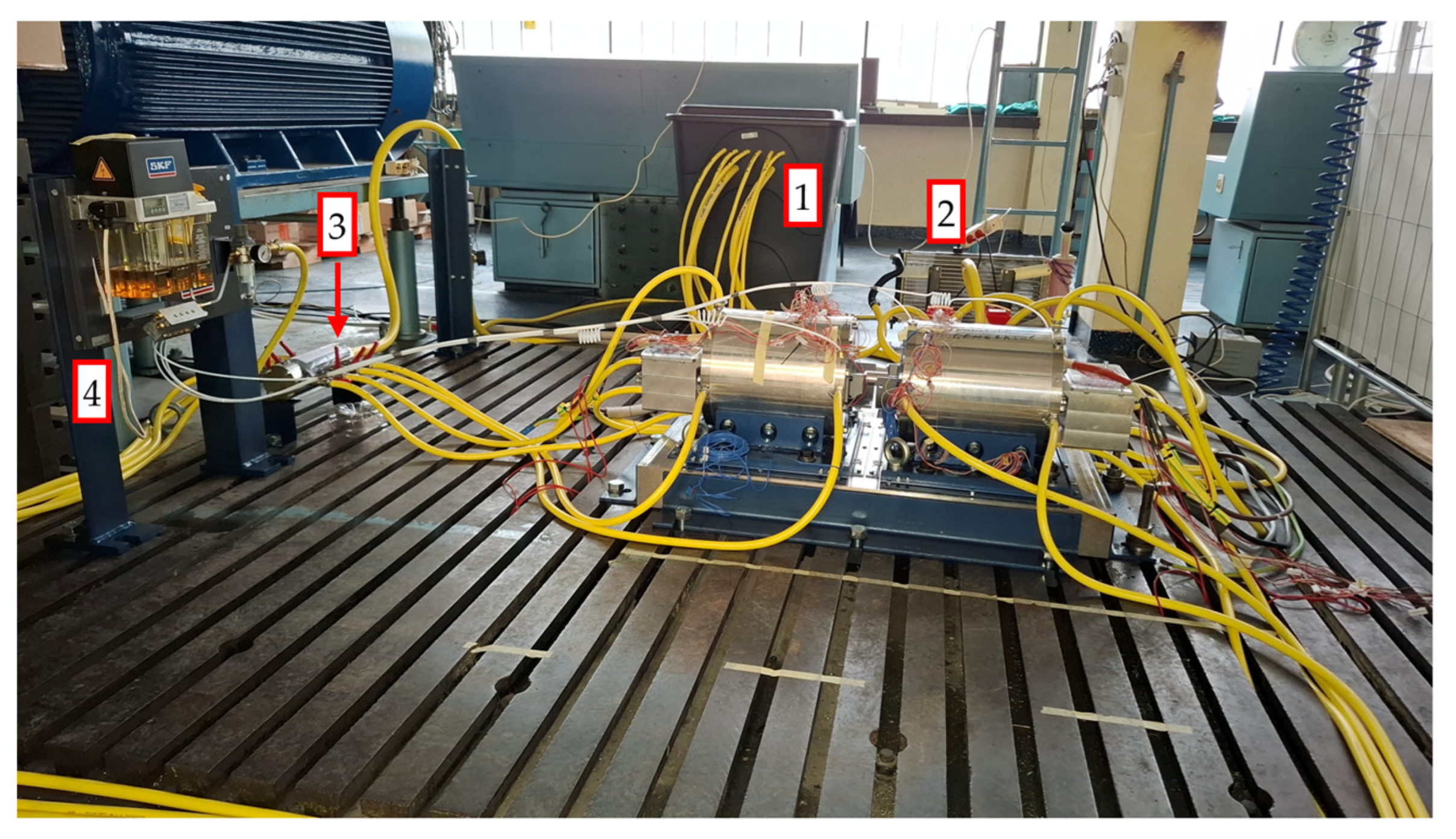
Figure 20.
Back-to-back testing setup for high-speed machine prototypes from the side. (1) Water tank, (2) radiator, (3) coolant splitter, (4) oil–air mist lubrication system.
Figure 20.
Back-to-back testing setup for high-speed machine prototypes from the side. (1) Water tank, (2) radiator, (3) coolant splitter, (4) oil–air mist lubrication system.
Figure 21.
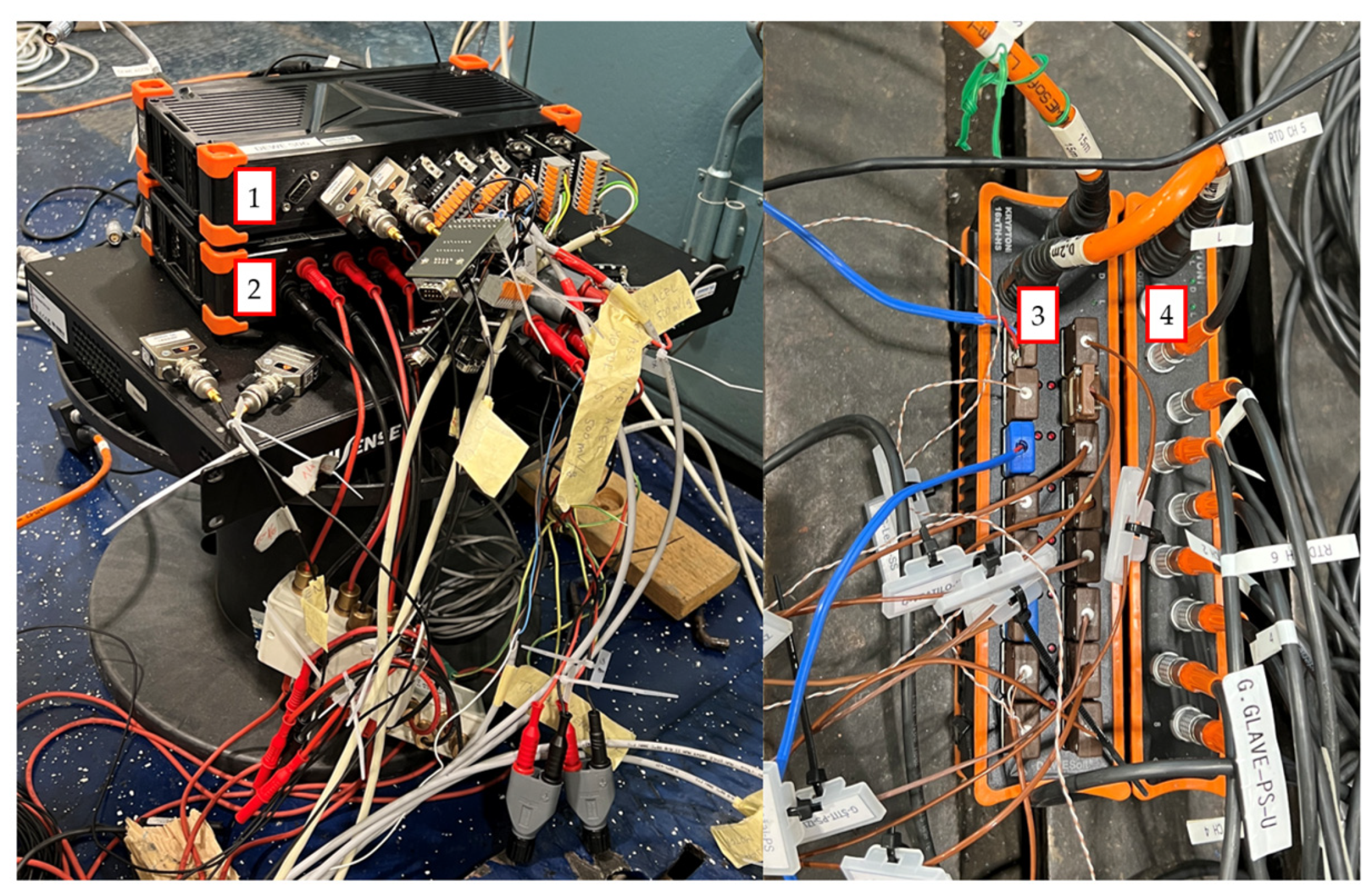
Acquisition system. (1) Dewesoft SIRIUS UNI, (2) Dewesoft SIRIUS XHS, (3) Dewesoft KRYPTON-TH-HS, (4) Dewesoft KRYPTON-RTD-HS.
Figure 21.
Acquisition system. (1) Dewesoft SIRIUS UNI, (2) Dewesoft SIRIUS XHS, (3) Dewesoft KRYPTON-TH-HS, (4) Dewesoft KRYPTON-RTD-HS.
Figure 22.
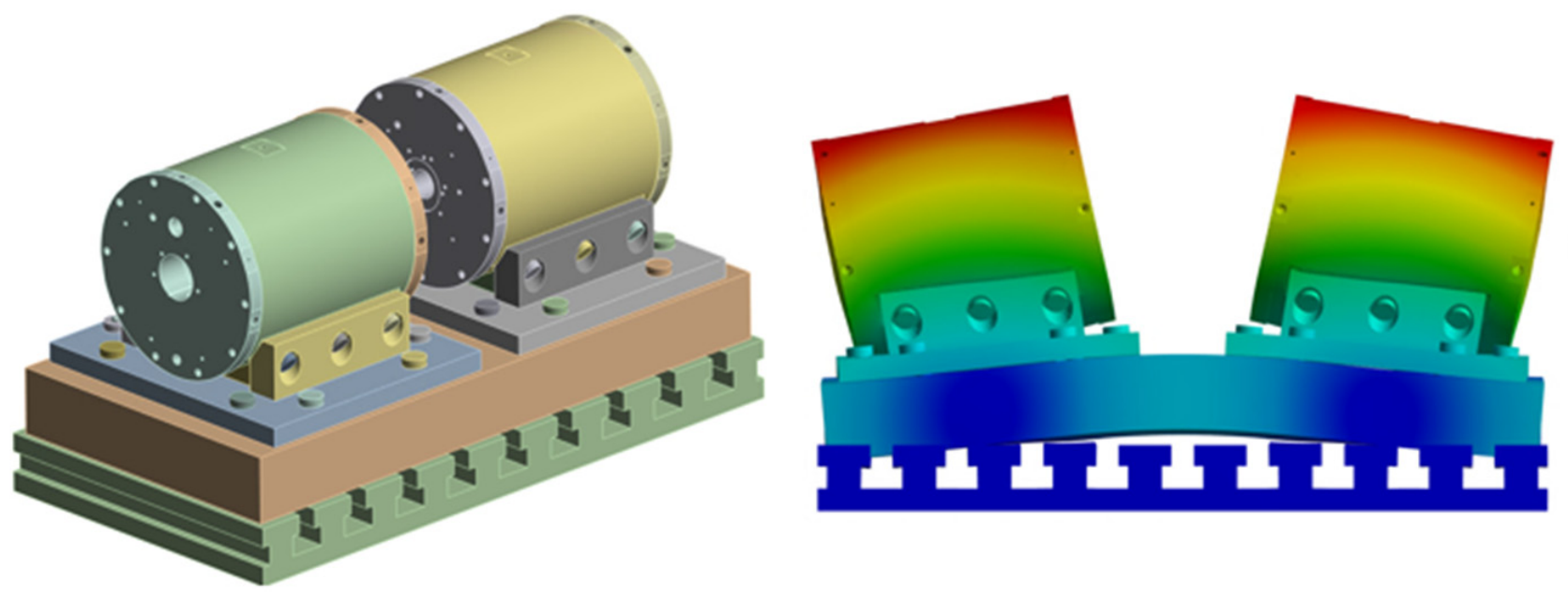
Simulated test bench vibration mode shape excited by second-order excitation at 15,000 rpm. The contour colors indicate the relative vibration displacement amplitude of the mode shape, with red regions representing maximum displacements and blue regions representing minimum displacement.
Figure 22.
Simulated test bench vibration mode shape excited by second-order excitation at 15,000 rpm. The contour colors indicate the relative vibration displacement amplitude of the mode shape, with red regions representing maximum displacements and blue regions representing minimum displacement.
Figure 23.
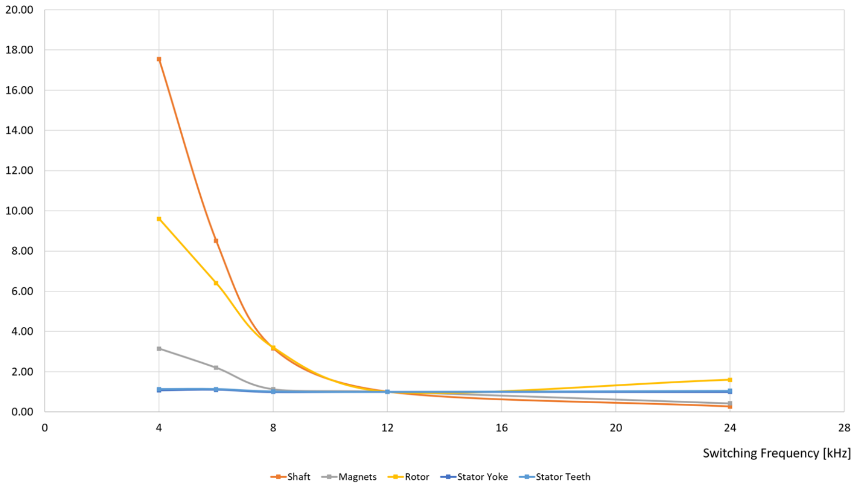
Machine losses versus PWM switching frequency in per-unit values (1 pu at 12 kHz).
Figure 23.
Machine losses versus PWM switching frequency in per-unit values (1 pu at 12 kHz).
Figure 24.
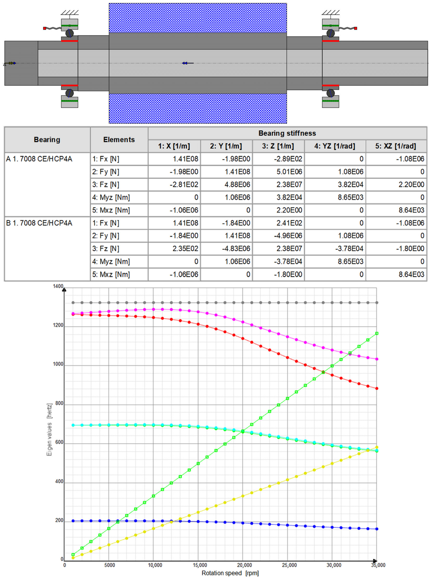
Concept modal analysis and the critical speed map. The left arrow on top figure represents the direction of rotation, the right arrow represents the torque direction. The colors on the bottom diagram are as follows: the axial vibration mode at 205 Hz (dark blue), the first bending mode at 625 Hz at 25,000 rpm (cyan), the first-order electromagnetic excitation (inclined yellow), the second-order electromagnetic excitation (inclined green).
Figure 24.
Concept modal analysis and the critical speed map. The left arrow on top figure represents the direction of rotation, the right arrow represents the torque direction. The colors on the bottom diagram are as follows: the axial vibration mode at 205 Hz (dark blue), the first bending mode at 625 Hz at 25,000 rpm (cyan), the first-order electromagnetic excitation (inclined yellow), the second-order electromagnetic excitation (inclined green).
Figure 25.
Detailed FEM-based machine modal analysis. The contour colors indicate the relative vibration displacement amplitude of the mode shape, with red regions representing maximum displacements on the rotor and blue regions representing minimum displacements on the stator and housing.
Figure 25.
Detailed FEM-based machine modal analysis. The contour colors indicate the relative vibration displacement amplitude of the mode shape, with red regions representing maximum displacements on the rotor and blue regions representing minimum displacements on the stator and housing.
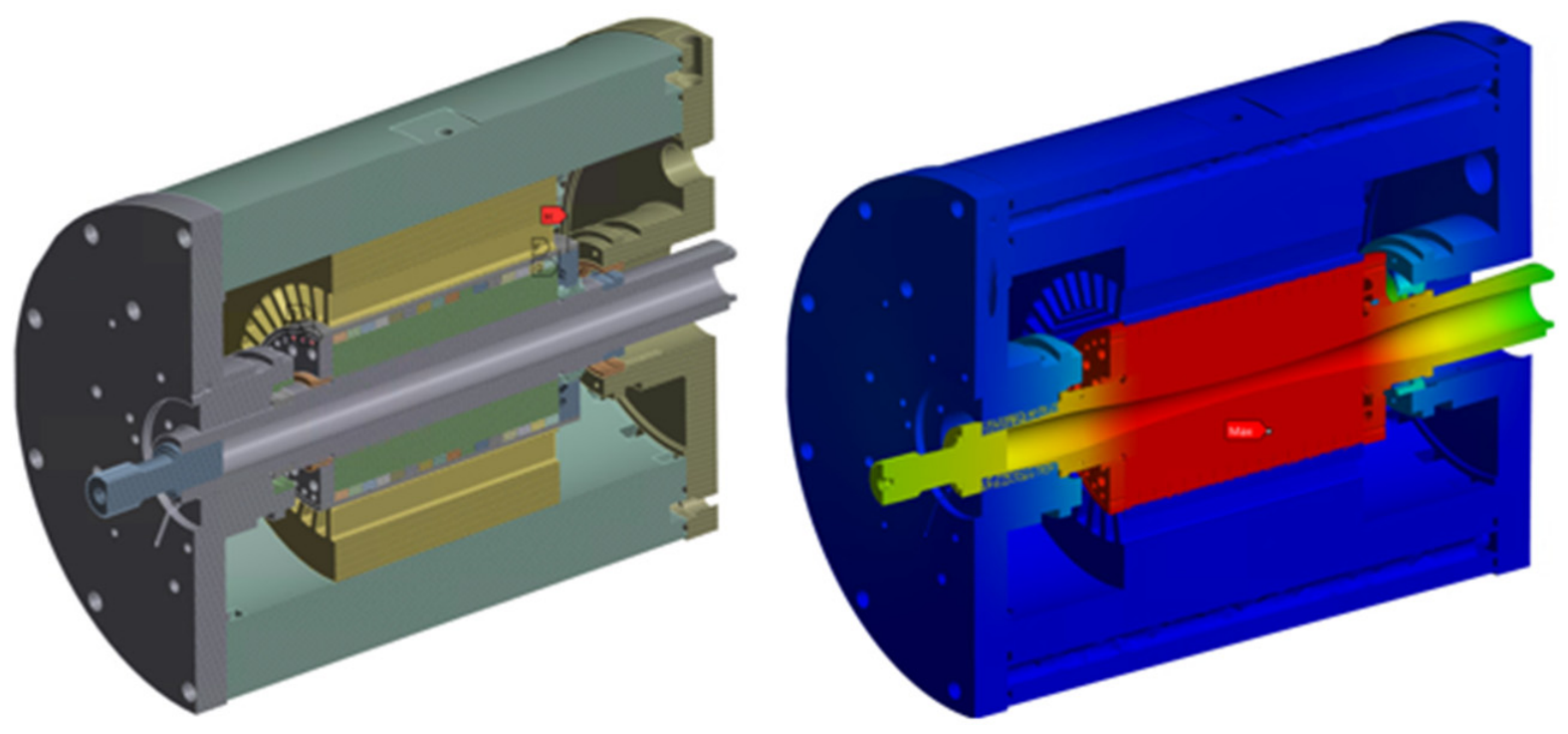
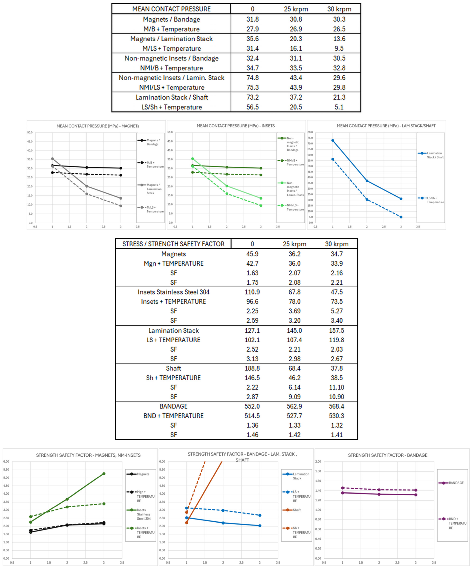
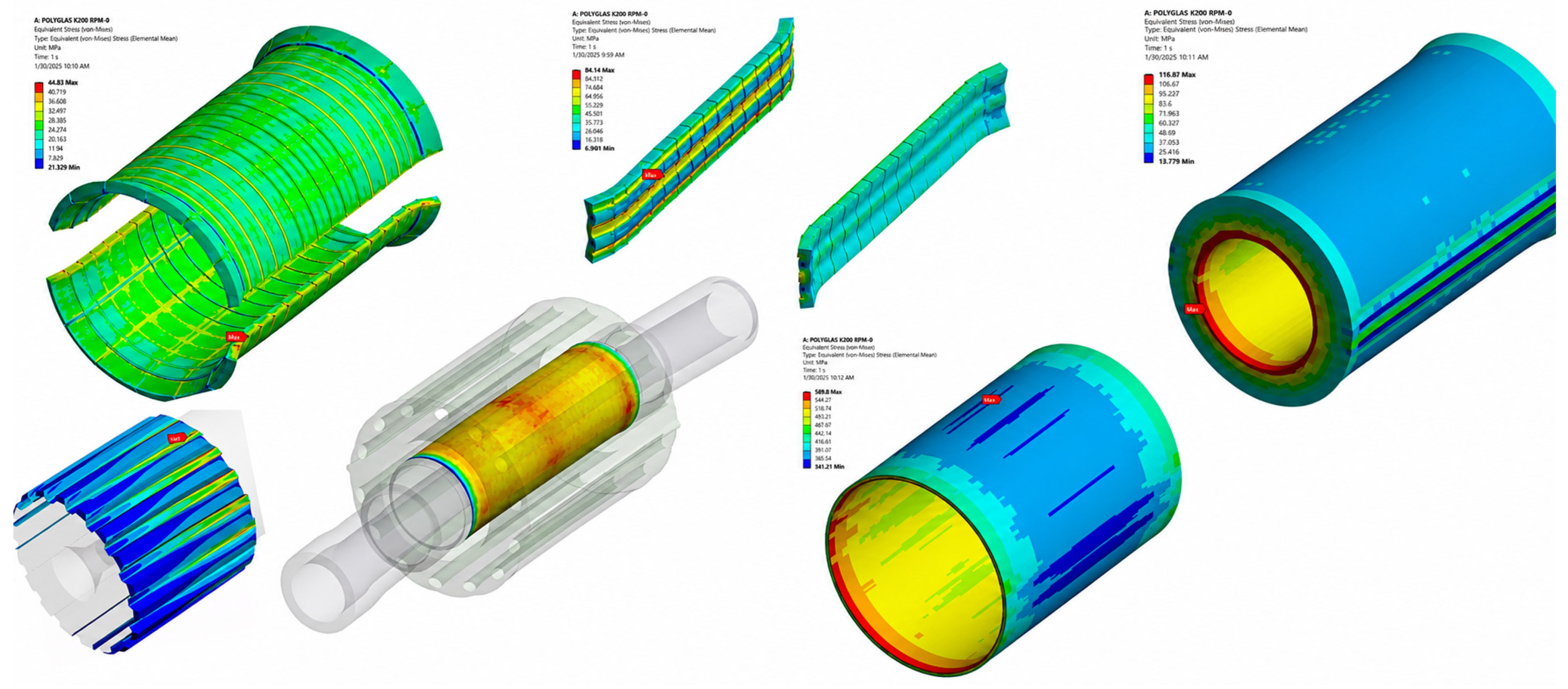
Figure 26.
Operational contact safety, stresses and the strength safety factors.
Figure 26.
Operational contact safety, stresses and the strength safety factors.
Figure 27.
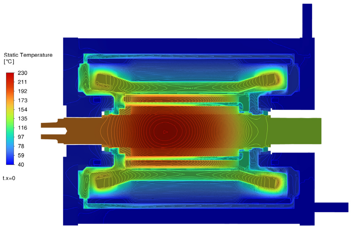
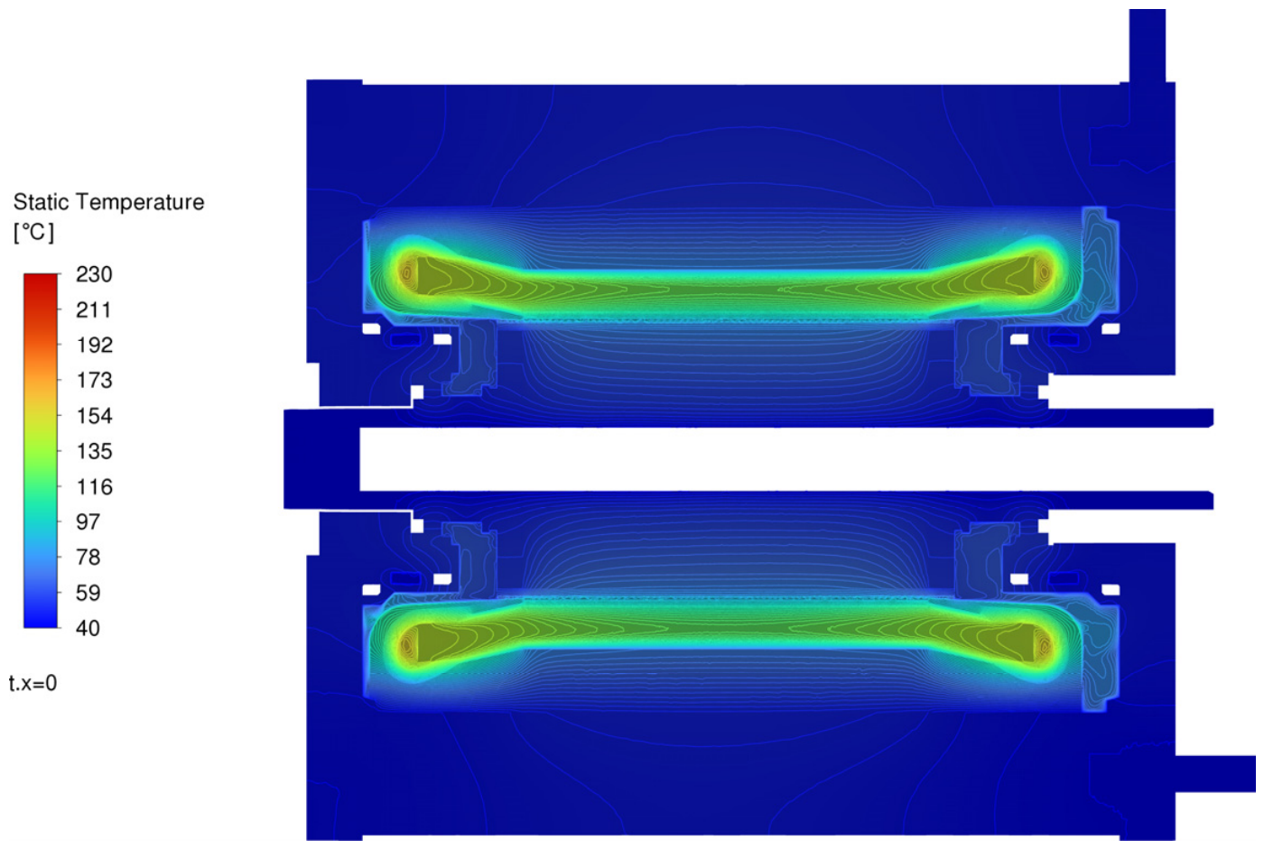
Temperature contours resulting from a steady-state 3D CHT model in sine wave operating conditions.
Figure 27.
Temperature contours resulting from a steady-state 3D CHT model in sine wave operating conditions.
Figure 28.
Temperature contours resulting from a steady-state 3D CHT model in power converter operating conditions.
Figure 28.
Temperature contours resulting from a steady-state 3D CHT model in power converter operating conditions.
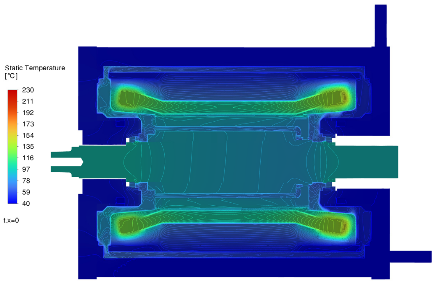
Figure 29.
Temperature contours resulting from a steady-state 3D CHT model in power converter operating conditions with a water-cooled hollow shaft.
Figure 29.
Temperature contours resulting from a steady-state 3D CHT model in power converter operating conditions with a water-cooled hollow shaft.
Figure 30.
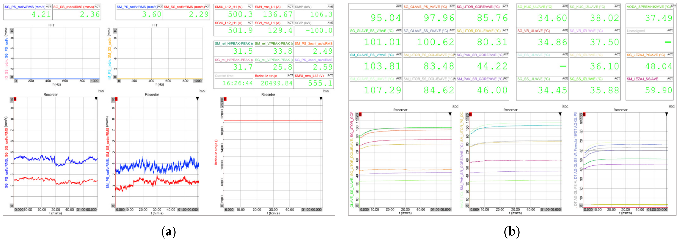
Measurements performed on synchronous machines (100 kW at 20,500 rpm). (a) Vibrations and electrical quantities, (b) temperatures. Figure (a) illustrates the generator radial vibrations at the DE (blue) and NDE (red) on the left, the motor radial vibrations at the DE (blue) and NDE (red) in the middle, and the operating speed on the right. Figure (b) displays the temperatures, where the left graph tracks the generator temperatures [end-windings (dark green, grey, red, white), slots (dark red, yellow), DE bearing (orange), and stator outer diameter (violet)], the middle graph tracks the motor temperatures [end-windings (light green, turquoise), slots (grey, orange), NDE bearing (magenta), and stator outer diameter (violet)], and the right graph displays the calculated temperature rises relative to the absolute values.
Figure 30.
Measurements performed on synchronous machines (100 kW at 20,500 rpm). (a) Vibrations and electrical quantities, (b) temperatures. Figure (a) illustrates the generator radial vibrations at the DE (blue) and NDE (red) on the left, the motor radial vibrations at the DE (blue) and NDE (red) in the middle, and the operating speed on the right. Figure (b) displays the temperatures, where the left graph tracks the generator temperatures [end-windings (dark green, grey, red, white), slots (dark red, yellow), DE bearing (orange), and stator outer diameter (violet)], the middle graph tracks the motor temperatures [end-windings (light green, turquoise), slots (grey, orange), NDE bearing (magenta), and stator outer diameter (violet)], and the right graph displays the calculated temperature rises relative to the absolute values.
Table 1.
Standardized parts used to build the machine.
Table 1.
Standardized parts used to build the machine.
| Component | Type |
|---|
| Casing | IEC 160 for water cooling |
| Lamination cut | IEC 160/2.135 |
| Lamination steel | 0.5 mm M270-50A |
| Squirrel cage | Cast aluminum |
| Wire | Enameled copper round size 0.85 mm |
| Bearing | 6307 M/C4 Ball bearing |
Table 2.
Main geometry data of the simulated induction and permanent magnet machines.
Table 2.
Main geometry data of the simulated induction and permanent magnet machines.
| | Parameter | Value |
|---|
| BOTH | Stator outer diameter | 200 mm |
| Stator inner diameter | 110 mm |
| Stator slots | 36 |
| Air gap | 1 mm |
| Axial length | 160 mm |
| Shaft inner diameter | 25 mm |
| IM | Rotor slots | 30 |
| Shaft outer diameter | 50 mm |
| PM | Rotor banding thickness | 3 mm |
| Magnet thickness | 5.5 mm |
| Magnet arc | 150° |
| Magnet grade | N30EH |
| Shaft outer diameter | 55 mm |
Table 3.
Main data of the coupled simulation.
Table 3.
Main data of the coupled simulation.
| Parameter | Value |
|---|
| DC link voltage | 750 V |
| Switching frequency | 12.5 kHz |
| Peak current (1st harmonic) | 180 A |
| Phase advance angle | 17° |
Table 4.
Comparison between measured and simulated data.
Table 4.
Comparison between measured and simulated data.
| | Measured | Simulated |
|---|
| Phase voltage [V] | 306.5 | 305.7 |
| Phase current [A] | 119.5 | 130.3 |
| Power factor [-] | 0.82 | 0.86 |
| Slip [%] | 0.7509 | 0.6112 |
| Shaft power [kW] | 93.11 | 94.60 |
| Total loss [kW] | 7.89 | 7.75 |
Table 5.
Simulation results for sine wave excitation.
Table 5.
Simulation results for sine wave excitation.
| Simulation Output | 15 krpm | 20 krpm | 25 krpm |
|---|
| RMS current [A] | 121 | 121 | 121 |
| Torque [Nm] | 38.7 | 39.5 | 38.6 |
| Armature copper loss [W] | 1182 | 1182 | 1182 |
| Rotor cage loss [W] | 592 | 605 | 618 |
| Stator yoke loss [W] | 287 | 420 | 568 |
| Stator teeth loss [W] | 164 | 260 | 380 |
| Rotor iron loss [W] | 167 | 290 | 445 |
| Shaft loss [W] | 0.1 | 0.1 | 0.1 |
| Mechanical loss [W] | 210 | 342 | 528 |
| Stray loss [W] | 602 | 801 | 997 |
Table 6.
Measurement and simulation results at 14,000 rpm for an induction machine prototype.
Table 6.
Measurement and simulation results at 14,000 rpm for an induction machine prototype.
| Simulation Output | Simulated | Measurement |
|---|
| Phase voltage (1st harm.) [V] | 169.7 | 169.2 |
| Phase current (1st harm.) [A] | 112.8 | 120.0 |
| Power factor (1st harm.) [-] | 0.92 | 0.88 |
| Slip [%] | 0.8486 | 0.9859 |
| Shaft power [kW] | 53.3 | 52.4 |
| Total loss [kW] | 2.90 | 2.97 |
Table 7.
Simulation results for sine and PWM excitation at 25,000 rpm.
Table 7.
Simulation results for sine and PWM excitation at 25,000 rpm.
| Simulation Output | Sine | PWM |
|---|
| RMS current [A] | 140 | 143 |
| Torque [Nm] | 44.9 | 45.9 |
| Copper loss [W] | 1585 | 1650 |
| Stator yoke loss [W] | 445.9 | 454.3 |
| Stator teeth loss [W] | 143.3 | 182.7 |
| Rotor yoke loss [W] | 0.03 | 3.4 |
| Magnet loss [W] | 26.9 | 146.5 |
| Shaft loss [W] | 0.4 | 671.9 |
Table 8.
Component maximum temperature in case of sine wave and power converter operation.
Table 8.
Component maximum temperature in case of sine wave and power converter operation.
| Component | Tmax, sine [°C] | Tmax, PWM [°C] | Tmax, PWM, WC [°C] |
|---|
| End Windings | 150 | 163 | 149 |
| Slot Windings | 119 | 137 | 131 |
| Stator Yoke | 84 | 98 | 89 |
| Stator Teeth | 99 | 133 | 109 |
| Rotor Yoke | 89 | 211 | 76 |
| Magnets | 93 | 191 | 83 |
| Shaft | 87 | 223 | 59 |
| Bearings | 100 | 182 | 60 |
Table 9.
Measurement and simulation results at 14,000 rpm for a PM machine prototype.
Table 9.
Measurement and simulation results at 14,000 rpm for a PM machine prototype.
| Simulation Output | Sine | PWM | Measurement |
|---|
| Phase voltage (1st harm.) [V] | 203.2 | 213.1 | 202.8 |
| Phase current (1st harm.) [A] | 116.5 | 128.9 | 121.8 |
| Power factor (1st harm.) [-] | 0.90 | 0.80 | 0.86 |
| Shaft power [kW] | 63.3 | 62.9 | 63.2 |
| Total loss [kW] | 2.01 | 2.34 | 2.49 |
Table 10.
Measurement and simulation results at 20,500 rpm for a PM machine prototype.
Table 10.
Measurement and simulation results at 20,500 rpm for a PM machine prototype.
| Simulation Output | Simulated | Measurement |
|---|
| Phase voltage (1st harm.) [V] | 326.6 | 290.6 |
| Phase current (1st harm.) [A] | 133.2 | 129.8 |
| Power factor (1st harm.) [-] | 0.97 | 0.89 |
| Shaft power [kW] | 101.8 | 100.2 |
| Total loss [kW] | 3.31 | 3.05 |
Table 11.
Comparison of machine prototypes.
Table 11.
Comparison of machine prototypes.
| Parameter | P1 | P2-IM | P2-SPM |
|---|
| Total active mass [kg] | 76.1 | 32.7 | 32.1 |
| Stator outer diameter [mm] | 240 | 200 | 200 |
| Rotor outer diameter [mm] | 133.4 | 108 | 102 |
| Axial length [mm] | 250 | 160 | 160 |
| Operating speed [rpm] | 13,000 | 14,000 | 14,000 | 20,500 |
| Operating frequency [Hz] | 216 | 233.33 | 233.33 | 341.67 |
| Mechanical power [kW] | 93.1 | 52.4 | 63.2 | 100.0 |
| Current [A] | 119.5 | 120 | 121.8 | 129.4 |
| Efficiency [%] | 92.19 | 94.64 | 96.21 | 97.04 |
| Water inlet temperature [°C] | 17.5 | 31 | 31.5 | 34.5 |
| End-winding temperature [°C] | 122 | 107 | 87.5 | 101 |
| Stator slot temperature [°C] | - | 79 | 72 | 83 |
| Outer stator area temperature [°C] | 42 | 39 | 39 | 44 |
| Bearing max. temperature [°C] | 90 | 45 | 38 | 48 |
| Radial vibration at DE [mm/s] | 0.60 | 0.38 | 1.65 | 4.21 |
| Radial vibration at NDE [mm/s] | 1.45 | 0.48 | 0.49 | 2.36 |




 ,
,