DHMGAT: A Dynamic and Hierarchical Multi-Head Graph Attention Network for Fault Location in Distribution Networks

Abstract

Fault location in distribution networks is challenged by dynamic topology changes and heterogeneous equipment. This paper proposes a Dynamic and Hierarchical Multi-Head Graph Attention Network (DHMGAT) that overcomes the limitations of static graph assumptions. Unlike methods that treat network structure as fixed or neglect line parameters, DHMGAT employs a hierarchical multi-head attention mechanism to encode topology dynamically. An Edge Feature Encoding Module fuses physical line attributes—impedance and switch states—directly into node embeddings. A Topology-Gated Pooling mechanism adapts to radial structural variations, and a Physics-Constrained Data Augmentation strategy ensures robustness under limited-sample and anomalous-data conditions. Evaluated on the IEEE 33-node and IEEE 123-node systems under comprehensive fault scenarios, DHMGAT achieves localization accuracies of 96.70% and 94.31%, respectively, with near-perfect calibration (ECE = 0.066). It maintains accuracy above 92% under high-noise conditions and N-1 topological reconfiguration, and above 88% under severe feature loss (up to 30% missing data), substantially outperforming conventional graph neural networks.

1. Introduction

Distribution networks are undergoing a fundamental transformation driven by the global transition to low-carbon energy and the large-scale integration of renewable sources. The widespread deployment of distributed photovoltaics, energy storage systems, and electric vehicle charging infrastructure is converting traditional unidirectional radial networks into active distribution systems characterized by multi-source coordination and bidirectional power flows [1,2]. While this shift improves energy efficiency and operational flexibility, it also introduces highly complex fault characteristics and propagation mechanisms. Frequent network reconfigurations, dynamic topology changes, and a growing share of power electronic devices make rapid and accurate fault location a critical technical challenge for safe and reliable distribution system operation [3].

Traditional fault location methods rely primarily on analytical techniques based on physical models. The impedance method [4] estimates fault distance by measuring the equivalent impedance of the faulted circuit. However, its accuracy is strongly affected by line parameter precision, transient resistance, and system operating conditions. The traveling wave method [5] offers high accuracy in theory. Yet it imposes stringent requirements on sampling equipment and faces challenges in wavefront identification and wave velocity determination, especially in multi-branch distribution networks. Methods based on voltage sags [6] and fault recording data analysis [7] depend on comprehensive system models and accurate network parameters, and they lack adaptability to dynamically changing topologies. These conventional approaches all exhibit significant limitations in systems with high-penetration distributed energy resources, necessitating new intelligent fault-location technologies that can adapt to dynamic changes in network structure [8].

In recent years, deep learning has brought new opportunities to distribution network fault location. Sirojan et al. [9] proposed a high-impedance fault detection method based on a convolutional deep neural network, constructing two-dimensional feature maps via wavelet packet entropy to locate high-impedance faults. To capture the dynamic characteristics of fault transients, Zhou et al. [10] introduced a Gated Recurrent Unit (GRU) network to model voltage time-series from multiple measurement points, significantly improving localization robustness under complex fault scenarios. Bidirectional Long Short-Term Memory (BiLSTM) networks [11] with graph-aware node ordering provide an alternative sequence-based approach, capturing sequential dependencies in bus measurements. However, their spatial reasoning capacity is limited by the arbitrary ordering of graph nodes, since LSTM layers inherently operate on linear sequences rather than irregular graph structures. Zeng et al. [12] proposed converting three-phase voltage and current time-series into two-dimensional images via Gramian Angular Fields (GAFs) and combining them with an improved deep residual network incorporating attention mechanisms and regularization for feature learning and fault detection, achieving strong performance under high-noise and small-sample conditions.

Despite their promise, these methods share a fundamental limitation: they treat each node’s measurements as independent time-series samples or forcibly reshape them into grid-like structures via sliding windows [13]. While this facilitates the use of established models such as CNNs and RNNs, it severs the intrinsic topological correlations formed by physical line connections. A distribution network is fundamentally a spatial graph of buses (nodes) and branches (edges), along which faults propagate and couple. In extreme cases, failures initiated by a few components can cascade across the network, leading to large-scale blackouts [14]. Methods based on CNNs or RNNs do not exploit this graph-structured prior, discarding critical spatial information and fault-propagation mechanisms during training. This creates generalization bottlenecks when modeling complex topological coupling [15] and long-distance propagation paths [16].

To address these non-Euclidean data structures, Graph Neural Networks (GNNs) [17,18] have emerged as a powerful tool for analyzing networked systems. The core mechanism of GNNs is message passing [19], which enables each node to update its state by aggregating information from neighboring nodes. This process is naturally aligned with the physical propagation of grid disturbances along transmission lines [20]. In early work, Chen et al. [21] applied Graph Convolutional Networks (GCNs) to fault location in radial distribution networks, encoding network topology into adjacency matrices and demonstrating the potential of graph-structured information. Hu et al. [22] proposed a fault diagnosis framework based on Spatio-Temporal Graph Convolutional Networks (STGCNs), integrating physical topological constraints with spatio-temporal convolution modules for multi-task collaborative learning of fault location and type identification. Subsequently, more advanced GNN variants such as GraphSAGE [23] and Graph Attention Networks (GATs) [24] were introduced to better handle heterogeneous node features and differences in neighbor importance.

Several attention-based refinements have been proposed on the GAT backbone. GATv2 [25] addresses the static-attention limitation of the original GAT by applying the weighting function after the nonlinearity, enabling strictly more expressive neighbor weighting. GATTransformer [26] combines transformer-style global self-attention with GNN message passing, allowing each node to attend to all others and thereby capture long-range dependencies that multi-hop GAT layers may dilute. While these models enhance the representational capacity of attention-based graph learning, they retain the standard node-only message-passing paradigm and do not incorporate edge-level physical features such as line impedance or switch states.

A separate line of work has sought to integrate edge information into GNN architectures. GINE [27] extends the Graph Isomorphism Network (GIN) with a learnable edge feature integration mechanism during message passing, providing a theoretically grounded framework for incorporating edge attributes. More directly relevant to the power domain, Edge-Enhanced GAT (EGAT) [28] fuses line impedance and admittance directly into the attention coefficient computation, achieving superior performance on tasks where branch parameters critically influence fault current distribution. Among existing methods, EGAT is the strongest single-task competitor and demonstrates that edge-aware attention can substantially improve fault localization accuracy.

Nonetheless, even EGAT operates without a hierarchical pooling mechanism to capture radial structural variations. Furthermore, existing GNN-based methods—including EGAT—have primarily been validated on small-scale networks, leaving their scalability and topological transferability to larger, more realistic systems underexplored. These gaps motivate the need for a comprehensive framework that jointly addresses edge feature encoding, multi-scale topology adaptation, and large-scale validation within a unified architecture.

Despite these advances, most current GNN models for fault location still face two unresolved challenges. The first is the insufficient integration of physical information. Existing studies typically simplify the network into a graph of connectivity only, using a binary adjacency matrix to define edges. This simplification ignores the physical attributes of transmission lines—impedance, ground capacitance, length, and real-time switching states [29]—which are the core factors determining fault current distribution, voltage sag magnitude, and protection device behavior. Sun et al. [30] showed that GNN models without branch parameters cannot effectively distinguish fault scenarios with similar electrical characteristics but different branch parameters, limiting localization accuracy in complex distribution networks.

The second challenge is the limited ability to handle dynamic topological changes. To optimize operation, isolate faults, or accommodate renewable energy, practical distribution networks undergo regular reconfiguration through sectionalizing and tie switches [31], causing dynamic or abrupt changes to their graph structures. Most GNN models learn information propagation patterns closely tied to the training topology, leading to a risk of “topological overfitting”. When the model encounters a topology unseen during training, its performance can suffer catastrophic degradation—a problem known as the “topological generalization gap”. Liu et al. [32] confirmed that standard GCN and GAT models exhibit significant accuracy declines on test sets with topological variations. These models also fail to produce feasible AC-OPF solutions, severely restricting their deployment in real dynamic distribution networks. Wu et al. [33] proposed the Universal Graph Convolutional Network (UGCN) to improve generalization via shared feature representation and parallel decoding for zero-shot transfer to unknown topologies. However, the adaptive output module increases model complexity and training cost, and generalization performance still degrades when the base system’s topological features differ substantially from those in extreme reconfiguration scenarios.

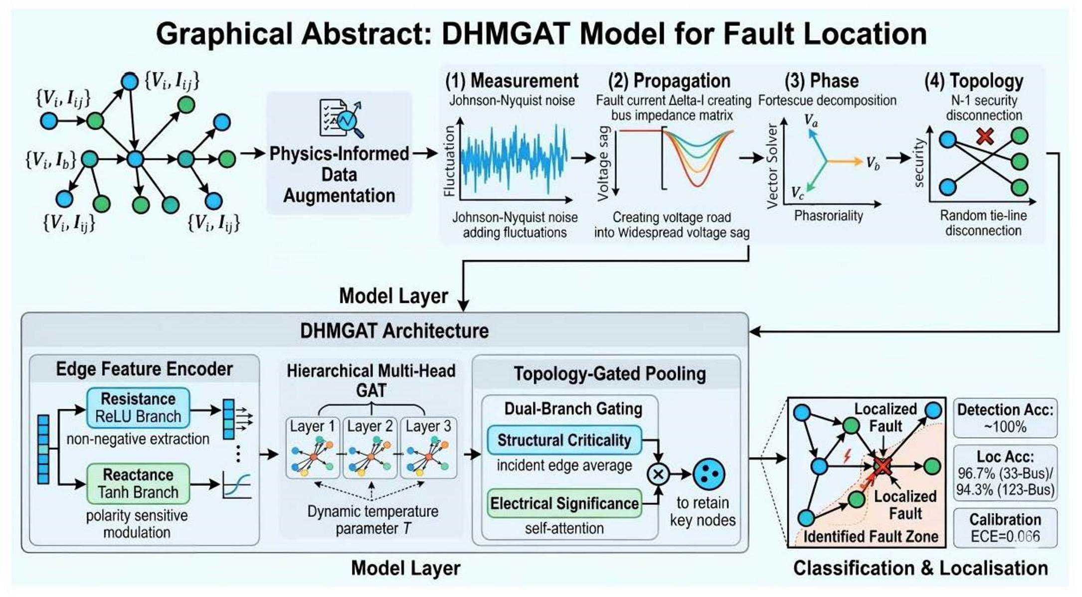
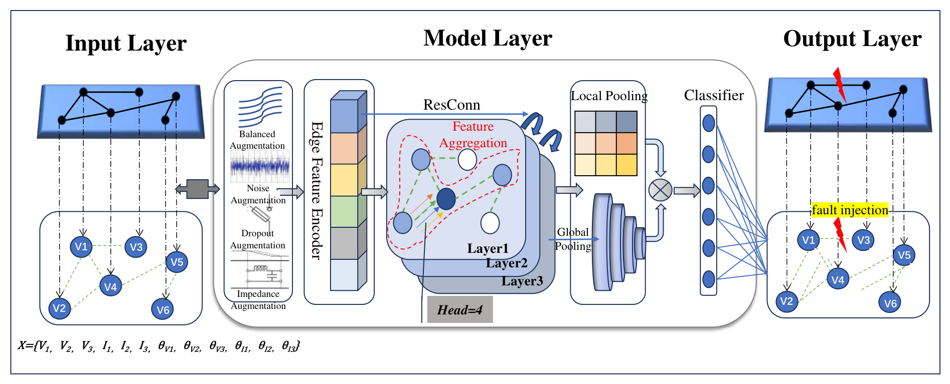
To address these challenges, this paper proposes DHMGAT. The core idea is to embed the physical characteristics and topological dynamics of distribution networks into the GNN architecture and training process, guiding the model to learn fundamental fault propagation laws beyond specific wiring diagrams. The main contributions are:

• Polarity-Aware Edge Encoding: Unlike existing methods that fuse line impedance through a single linear projection (e.g., EGAT [28]), we design a dual-channel encoder that applies ReLU to the resistance-dominated component and Tanh to the reactance-dominated component separately. The Tanh branch provides a polarity-sensitive modulation that is physically aligned with the sign of branch reactance, enabling the model to distinguish capacitive (negative reactance) from inductive branches. While this does not enforce a hard sign constraint due to the learnable projections, it introduces a soft inductive bias that guides the network to leverage reactance polarity—a critical factor in fault current distribution that standard single-channel encoders discard.
• Topology-Gated Hierarchical Attention: Rather than relying on uniform multi-layer stacking that dilutes local specificity as receptive fields grow, we propose a three-level attention pyramid with a dynamic temperature parameter $\tau$ that sharpens attention at the local level and softens it globally. This is complemented by a dual-branch gating mechanism that jointly evaluates global topological criticality (via incident-edge averaging) and local electrical significance (via self-attention), fusing them through a Hadamard product so that a node is retained only if it is both structurally pivotal and electrically anomalous—a criterion uniquely suited to the radial attenuation patterns of distribution networks. Ablation experiments confirm that this module alone contributes a 2.36% improvement in localization accuracy.
• Physics-Constrained Augmentation, Calibration, and Cross-Network Transfer: We establish a systematic augmentation framework that jointly enforces physical constraints across four layers—measurement-layer thermal noise (Johnson–Nyquist), propagation-layer voltage perturbations (bus impedance matrix), phase-layer symmetrical components (Fortescue), and topology-layer compensation for N-1 contingencies—which is the first work to cover all four dimensions in distribution network fault location. MC Dropout is integrated natively (not as a post hoc step), providing well-calibrated confidence with ECE = 0.066. The resulting representations transfer to the IEEE 123-bus system with only 2.39 pp degradation and achieve 94.07% accuracy with one labeled sample per class via few-shot fine-tuning.

To systematically position our contributions relative to prior art, we audit existing fault-location methods against the four physical dimensions underlying our augmentation strategy: (i) measurement-layer noise, (ii) propagation-layer impedance, (iii) phase-layer coupling, and (iv) topology-layer reconfiguration. Pure data-driven methods (e.g., FCNN [34], LSTM [11]) treat each node independently and thus cover none of these dimensions. Standard GNNs like GCN [21] and GraphSAGE [23] utilize graph connectivity but omit physical line parameters (missing layers ii–iv). Attention-based variants such as GATv2 [25] and GATTransformer [26] enhance expressiveness yet still operate solely on node features without physical constraints. The closest competitor, EGAT [28], incorporates line impedance into attention computation (partially covering layer ii); however, it does not model sensor noise characteristics (layer i), enforce three-phase coupling laws (layer iii), nor simulate N-1 structural contingencies (layer iv). Other spatio-temporal frameworks [22] focus on sequential correlations but neglect hierarchical noise scaling with electrical depth and phase imbalance. Consequently, no prior study has systematically unified all four physical layers within a single augmentation framework.

Table 1. Research gap analysis: capability comparison across existing methods and the proposed DHMGAT.

Capability	GCN [21]	GAT [24]	GATv2 [25]	GraphSAGE [23]	EGAT [28]	GATTrans. [26]	Ours
Edge Physical Features	--	--	--	--	✓	∘	✓
Hierarchical Attention	--	∘	∘	--	∘	∘	✓
Topology-Aware Pooling	--	--	--	∘	--	--	✓
Measurement-Layer Noise	--	--	--	--	--	--	✓
Propagation-Layer Impedance	--	--	--	--	∘	--	✓
Phase-Layer Coupling	--	--	--	--	--	--	✓
Topology-Layer N-1 Contingency	--	--	--	--	--	--	✓
Uncertainty Calibration	∘	∘	∘	∘	∘	∘	✓
Large-Scale Validation	∘	∘	∘	✓	∘	∘	✓

Physics-constrained layers: measurement-layer noise, propagation-layer impedance, phase-layer coupling, and topology-layer N-1 contingency. ✓ = native/built-in support; ∘ = partial/can be extended/post hoc techniques exist; -- = not supported.

compares DHMGAT against representative methods across six capability dimensions. While several baselines partially support certain dimensions, only the proposed framework integrates all six within a unified architecture with built-in mechanisms—rather than relying on post hoc extensions.

The remainder of this paper is organized as follows: Section 2 introduces the graph modeling of distribution networks, formulates the fault location problem, and reviews the theoretical foundations of GAT. Section 3 details the DHMGAT framework. Section 4 presents experimental results on the IEEE 33-node and IEEE 123-node systems. Section 5 summarizes the key findings and discusses future work.

2. Preliminaries

This section outlines the mathematical modeling of distribution networks, defines the fault location problem within a graph learning framework, and reviews the theoretical foundations of Graph Attention Networks.

2.1. Graph Construction of Distribution Networks

To apply graph neural networks, the distribution network is modeled as a directed graph $\mathcal{G}=(\mathcal{V},\mathcal{E})$, where $\mathcal{V}$ denotes the set of N buses, and $\mathcal{E}$ represents the set of branches connecting these buses.

• Node Feature Matrix (X):

For each node $v_i$, the feature vector ${\mathit{x}}_i$ captures the electrical state via three-phase measurements: voltages $\{V_i^a,V_i^b,V_i^c\}$, currents $\{I_i^a,I_i^b,I_i^c\}$, and their corresponding phase angles $\{{\theta }_i^a,{\theta }_i^b,{\theta }_i^c\}$.

The global node feature matrix $X\in {\mathbb{R}}^{N\times d}$ is defined as $X={[{\mathit{x}}_1,{\mathit{x}}_2,\dots ,{\mathit{x}}_N]}^{\top }$.

• Edge Feature Matrix (E):

Unlike traditional GNNs that define edges solely by connectivity, accurate fault location requires physical line parameters. We define an edge feature set $E=\{e_{ij}\mid (v_i,v_j)\in \mathcal{E}\}$, where each feature vector $e_{ij}$ for the branch connecting $v_i$ and $v_j$ contains: (1) line impedance—resistance $R_{ij}$ and reactance $X_{ij}$; (2) topological status—switch state $s_{ij}\in \{0,1\}$, where 1 indicates a closed connection and 0 indicates an open or disconnected line.

2.2. Problem Formulation

The fault location task in a distribution network with dynamic topology is formulated as a multi-class node classification problem. Given real-time electrical measurements X, edge feature matrix E, and the dynamic graph structure ${\mathcal{G}}_t$, the objective is to learn a non-linear mapping f:

$$\widehat{Y}=f(X,E,{\mathcal{G}}_t;\Theta ),$$

(1)

where $\widehat{Y}={[{\widehat{y}}_1,{\widehat{y}}_2,\dots ,{\widehat{y}}_N]}^{\top }$ is the output probability vector, with ${\widehat{y}}_i$ representing the probability that node $v_i$ is the fault location. The model must robustly identify the faulted node $\widehat{k}={\arg \max }_i{\widehat{y}}_i$ even when the topology ${\mathcal{G}}_t$ varies due to switch operations.

2.3. Graph Attention Networks

Using a GAT as the backbone overcomes the fixed-weight limitation of GCNs by dynamically weighting neighbors via an attention mechanism, effectively capturing spatial correlations in non-Euclidean grid structures.

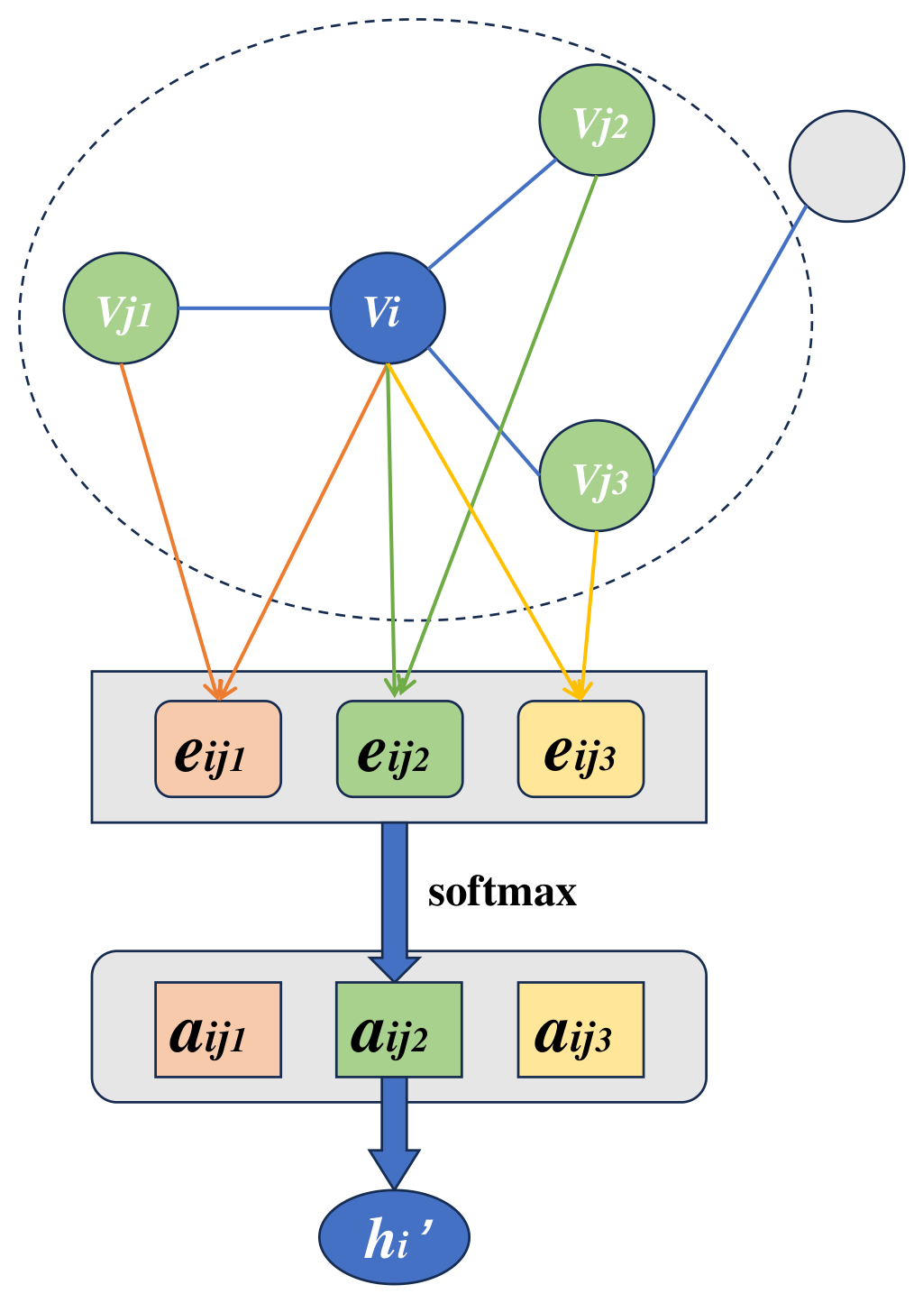
The core component is the Graph Attention Layer (GAL), which integrates attention mechanisms into the GNN framework. The neighbor information aggregation process in the GAT is illustrated in Figure 1. For node $v_i$, the importance of its neighbor $v_j$ is computed via a learnable attention coefficient ${\alpha }_{ij}$:

$${\alpha }_{ij}={\displaystyle \frac{\exp \left(\mathrm{LeakyReLU}\left({\mathit{a}}^{\top }[W{\mathit{h}}_i\parallel W{\mathit{h}}_j]\right)\right)}{{\sum }_{k\in {\mathcal{N}}_i}\exp \left(\mathrm{LeakyReLU}\left({\mathit{a}}^{\top }[W{\mathit{h}}_i\parallel W{\mathit{h}}_k]\right)\right)}},$$

(2)

where ${\mathit{h}}_i$ and ${\mathit{h}}_j$ represent the input feature vectors of node $v_i$ and $v_j$. $W\in {\mathbb{R}}^{d^{\prime }\times d}$ is a shared linear transformation matrix, $\mathit{a}\in {\mathbb{R}}^{2d^{\prime }}$ is the attention weight vector, and ‖ denotes concatenation.

To ensure numerical stability and comparability across nodes, coefficients are normalized by the softmax function:

$${\alpha }_{ij}={\mathrm{softmax}}_j\left(e_{ij}\right)={\displaystyle \frac{\exp \left(e_{ij}\right)}{{\sum }_{k\in {\mathcal{N}}_i}\exp \left(e_{ik}\right)}},$$

(3)

The final representation of node $v_i$ is updated by aggregating the weighted features of its neighbors:

$${\mathit{h}}_i^{\prime }=\sigma \left(\sum _{j\in {\mathcal{N}}_i}{\alpha }_{ij}W{\mathit{h}}_j\right),$$

(4)

where $\sigma$ is a non-linear activation function.

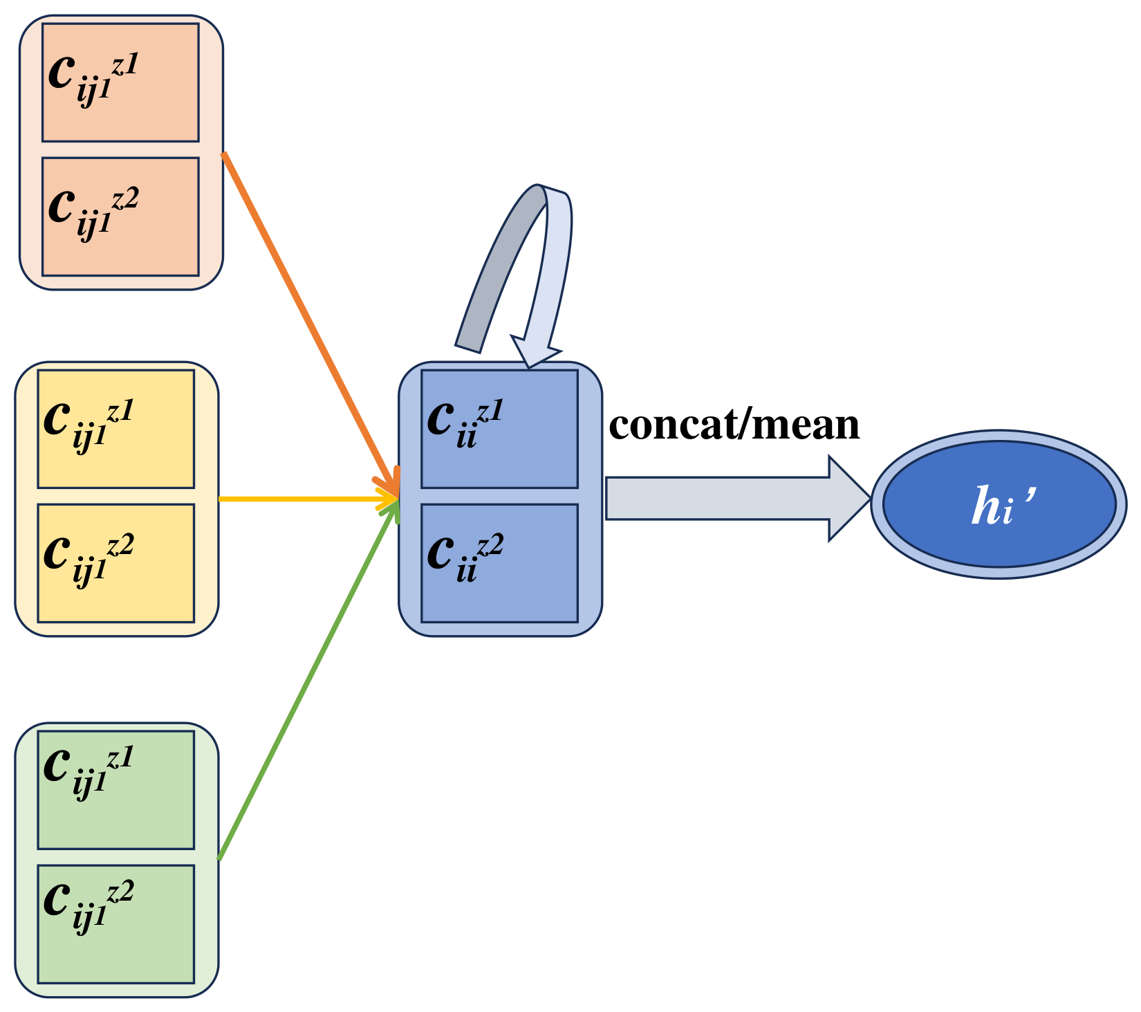
To further enhance stability and representation capacity, GAT employs multi-head attention, where z independent heads compute attention coefficients to capture diverse subspace features. In intermediate layers, concatenation is used to enhance representational power, though this increases feature dimensionality. The final layer therefore averages the outputs of multiple heads. As shown in Figure 2 ($z=2$), two independent attention modules work collaboratively to assign clearer, more discriminative weights to neighboring nodes, improving learning capability while reducing overfitting risk.

Compared with GCNs that rely on a fixed Laplacian matrix, GAT uses an adaptive weight matrix that dynamically adjusts inter-node coefficients. This enables GAT to assign differentiated weights to nodes at the same neighborhood depth. By considering the electrical characteristics of adjacent nodes simultaneously, GAT improves generalization in grid fault location tasks.

3. Proposed Methodology

This paper proposes DHMGAT, an end-to-end differentiable architecture for fault location in distribution networks with dynamic topologies. As illustrated in Figure 3, the model establishes a hierarchical representation learning pipeline that progressively aggregates features from local device interactions to global system states.

3.1. Heterogeneous Edge Feature Encoding

Distribution networks contain heterogeneous physical parameters, where continuous variables (line impedance) coexist with discrete states (switch status). Standard normalization fails to capture the nonlinear physical coupling between these modalities. To address this, we propose a Dual-Channel Feature Encoder that standardizes the dimensions of resistance and reactance while compressing their features [35]. Let the raw attribute vector for the edge connecting $v_i$ and $v_j$ be ${\mathit{e}}_{ij}^{\left(0\right)}={[R_{ij},X_{ij},s_{ij}]}^{\top }$. We map these attributes into a high-dimensional latent space using a physics-aware projection:

$${\mathit{e}}_{ij}=\mathrm{ReLU}\left(W_e^{\left(1\right)}{\mathit{e}}_{ij}^{\left(0\right)}+{\mathit{b}}_e^{\left(1\right)}\right)\odot \mathrm{Tanh}\left(W_e^{\left(2\right)}{\mathit{e}}_{ij}^{\left(0\right)}+{\mathit{b}}_e^{\left(2\right)}\right),$$

(5)

where $W_e^{\left(1\right)},W_e^{\left(2\right)}$ and ${\mathit{b}}_e^{\left(1\right)},{\mathit{b}}_e^{\left(2\right)}$ are learnable parameters.This dual-channel design serves two purposes. First, the ReLU branch extracts non-negative, resistance-sensitive features that reflect the magnitude of line losses. Second, the Tanh branch provides polarity-sensitive modulation that encourages the network to distinguish positive (inductive) from negative (capacitive) reactance contributions. The learnable projections do not rigidly preserve the sign of $X_{ij}$ after transformation. Nevertheless, applying an odd activation function (Tanh) on the second channel introduces a soft inductive bias. This bias aligns the latent representation with the physical polarity of reactance. This bias guides the attention mechanism to prioritize lines whose reactance sign is consistent with the expected fault propagation pattern, without requiring an explicit hard constraint.

3.2. Hierarchical Edge-Integrated Graph Attention

To capture fault signatures across varying topological scales—from local device interactions to system-wide energy states—we design a three-level attention pyramid. Unlike standard GATs that compute weights based solely on node similarity, our Edge-Integrated Attention Mechanism incorporates the edge embeddings derived in Section 3.

3.2.1. Edge-Integrated Attention Mechanism

The core innovation is the injection of physical line attributes into the attention scoring process. For a center node $v_i$ and its neighbor $v_j$, the attention coefficient ${\alpha }_{ij}^{\left(l\right)}$ at the l-th layer is computed as:

$$e_{ij}^{\left(l\right)}={\mathit{a}}^{{\left(l\right)}^{\top }}\mathrm{LeakyReLU}\left(W^{\left(l\right)}[{\mathit{h}}_i^{(l-1)}\parallel {\mathit{h}}_j^{(l-1)}\parallel {\mathit{e}}_{ij}]\right),$$

(6)

where $W^{\left(l\right)}$ is the linear transformation matrix, ${\mathit{a}}^{\left(l\right)}$ is the learnable attention vector, and ‖ denotes concatenation. To stabilize training, we employ multi-head attention with K independent heads. The final representation of node $v_i$ at layer l is:

$${\mathit{h}}_i^{\left(l\right)} = {\parallel }_{k=1}^K\sigma \left(\sum _{j\in {\mathcal{N}}_i}{\alpha }_{ij}^{(l,k)}{W}^{(l,k)}{\mathit{h}}_j^{(l-1)}\right),$$

(7)

where ${\alpha }_{ij}^{(l,k)}$ is the normalized attention weight for the k-th head, and ‖ denotes concatenation of multi-head outputs.

3.2.2. Hierarchical Feature Aggregation

Based on the mechanism above, the model progressively extracts features at three levels:

• Bottom layer (local interaction): The initial attention layers focus on 1-hop neighbors to capture fine-grained interactions between directly connected devices (e.g., voltage drops across a line segment). A dynamic temperature parameter $\tau$ is used in the softmax function to sharpen the attention distribution, distinguishing critical neighbors from noise.
• Middle layer (regional receptive field): Rather than relying on rigid electrical island partitioning—which fails under topological reconfiguration—we achieve regional aggregation by stacking multiple GAT layers. As network depth increases, each node’s receptive field expands to its k-hop neighborhood, allowing the model to dynamically perceive the status of the entire feeder section or local sub-region without manual intervention, ensuring robust performance even when tie switches alter the network structure.
• Top layer (global consensus): The final attention layer integrates information from the expanded receptive fields to capture global system states (e.g., total power balance, system-wide frequency deviations). This level ensures that local fault judgments remain consistent with global operational constraints.

3.3. Topological Gated Dynamic Pooling

Standard pooling strategies treat all nodes uniformly, often discarding critical radial structural information—particularly the voltage attenuation characteristics at terminal nodes. To address this, we propose a Topology-Gated Dynamic Pooling module with a Dual-Branch Gating Mechanism that simultaneously evaluates global topological context and local feature importance, as shown in Figure 3.

3.3.1. Global Gating Unit

The global gating unit integrates contextual information from both node features and edge embeddings. The topological branch focuses on structural connectivity, distinguishing critical bridge nodes from non-critical branches by aggregating the physical attributes of connected lines. Let $X\in {\mathbb{R}}^{N\times d}$ be the node feature matrix and $E\in {\mathbb{R}}^{M\times d_e}$ the edge feature matrix, where N is the number of nodes, M the number of edges, and d the feature dimension. We first compute a topological context vector ${\mathit{t}}_i$ for each node $v_i$ by averaging the embeddings of its incident edges:

$${\mathit{t}}_i={\displaystyle \frac{1}{|{\mathcal{N}}_i|}}\sum _{j\in {\mathcal{N}}_i}{\mathit{e}}_{ij},$$

(8)

where ${\mathcal{N}}_i$ denotes the neighbor set of node $v_i$, ${\mathit{e}}_{ij}$ represents the edge feature derived in Section 3, and $d_e$ is the edge feature dimension.

This representation is then concatenated with the node features and passed through a non-linear transformation to generate the global gating coefficient ${\mathit{g}}_i$:

$${\mathit{g}}_i=\sigma \left(W_g[{\mathit{x}}_i\parallel {\mathit{t}}_i]+{\mathit{b}}_g\right),$$

(9)

where $W_g$ is a learnable weight matrix, ${\mathit{b}}_g$ is the bias term, and $\sigma$ denotes the sigmoid activation function.

This mechanism effectively filters nodes by physical connectivity. It adaptively forms high-attention ring-like structures around fault locations to isolate anomalies.

3.3.2. Local Gating Unit

The local gating unit uses a multi-head attention mechanism to compute the local importance of each node, dynamically adjusting feature weights through learnable coefficients. It captures local electrical distance and feature significance via self-attention, ensuring that nodes with distinct fault signatures are prioritized regardless of topological position.

The query (Q), key (K), and value (V) matrices are derived from the node features X:

$$Q=X{W}_Q,K=X{W}_K,V=X{W}_V,$$

(10)

The attention weights for the h-th head are computed as:

$$A_h=\mathrm{softmax}\left({\displaystyle \frac{Q_h{K}_h^{\top }}{\sqrt{d_k}}}\right),$$

(11)

where $d_k$ is the feature dimension and H is the number of attention heads. The local importance vector ${\mathit{l}}_i$ is then obtained by aggregating the outputs of all H heads via a projection matrix $W_O$:

$${\mathit{l}}_i=\left[{\parallel }_{h=1}^H{A}_h{V}_h\right]W_O.$$

(12)

3.3.3. Hierarchical Aggregation

The outputs of the global and local gating units are fused via the Hadamard product. This design preserves both fine-grained structural characteristics and global operating states. A node is retained only if it is both topologically critical and electrically significant:

$${\mathit{s}}_i={\mathit{g}}_i\odot {\mathit{l}}_i,$$

(13)

where ⊙ denotes the Hadamard product. Finally, the graph-level representation ${\mathit{h}}_{\mathrm{graph}}$ is generated by the weighted aggregation of node features:

$${\mathit{h}}_{\mathrm{graph}}={\displaystyle \sum _{i=1}^N}{s}_i·{\mathit{h}}_i^{\left(L\right)},$$

(14)

where $s_i$ is the scalar gating score and ${\mathit{h}}_i^{\left(L\right)}$ is the final node representation from the last attention layer.

By integrating global topology with local feature details, this dynamic pooling strategy substantially enhances the model’s adaptability to the radial properties of distribution networks.

3.4. Physics-Informed Data Augmentation

To address the trade-off between data scarcity and physical consistency, we propose a multimodal augmentation strategy organized across four coupled physical layers: sensor noise characteristics (measurement layer), fault current propagation (propagation layer), three-phase coupling constraints (phase layer), and topological structural variation (topology layer). This ensures that augmented samples remain grounded in real electrical behavior. Each layer targets a distinct source of physical uncertainty in distribution network measurements, and together, they form a cohesive physics-constrained augmentation framework [36]. Crucially, all augmentation operations described in this section are applied exclusively to the training set. The validation and test sets remain in their original, unaugmented form to ensure unbiased evaluation of model performance.

• Hierarchy-aware noise injection (measurement layer): Field measurements are inherently corrupted by thermal noise, which is well described by the Johnson–Nyquist formula [37]. For a resistor R at temperature T with bandwidth B, the thermal noise voltage satisfies:

  $$\overline{v_n^2}=4k_{B}TRB,$$

  (15)

  where $k_B$ is the Boltzmann constant. In a radial distribution network, the cumulative resistance from the substation to a node $v_i$ grows with topological depth, i.e., $R_{\mathrm{cum}}\left(v_i\right)\propto \mathrm{depth}\left(v_i\right)$. Consequently, the noise standard deviation scales as $\sigma \left(v_i\right)\propto \sqrt{R_{\mathrm{cum}}\left(v_i\right)}$, which we approximate by a first-order linear expansion to make the augmentation computationally tractable:

  $${\tilde{V}}_i=V_i+ϵ·\left(1+\lambda ·\mathrm{depth}\left(v_i\right)\right),ϵ\sim \mathcal{N}(0,{\sigma }^2),$$

  (16)

  where $\lambda$ controls the depth-dependent amplification and $\sigma$ sets the base noise level. This formulation ensures that deeper nodes—which are electrically farther from the source and thus subject to greater signal attenuation and higher equivalent impedance—receive proportionally stronger noise, faithfully mirroring the spatial distribution of measurement uncertainty in practical feeder systems.
• Impedance-driven perturbation (propagation layer): In a multi-node power system, the relationship between fault current injection and the resulting voltage perturbation at all buses is governed by the bus impedance matrix ${\mathit{Z}}_{\mathrm{bus}}$ [38]. From the nodal voltage equation in phasor form $\tilde{\mathit{V}}={\mathit{Z}}_{\mathrm{bus}}\tilde{\mathit{I}}$, any change in injected current $\Delta \tilde{\mathit{I}}$ (e.g., due to a fault disturbance) propagates to a system-wide voltage change:

  $$\Delta \tilde{\mathit{V}}={\mathit{Z}}_{\mathrm{bus}}·\Delta \tilde{\mathit{I}},{\parallel \Delta \tilde{\mathit{V}}\parallel }_2\le \delta ,$$

  (17)

  where $\Delta \tilde{\mathit{I}}\in {\mathbb{R}}^{3N}$ represents the three-phase fault injection current vector (non-zero only at the faulted node), ${\mathit{Z}}_{\mathrm{bus}}\in {\mathbb{R}}^{3N\times 3N}$ is the three-phase bus impedance matrix encoding line impedances and transformer couplings, and $\delta$ is a perturbation bound that preserves the small-signal linearity assumption. By sampling $\Delta \tilde{\mathit{I}}$ within a physically plausible range (e.g., $\pm 0.1$ p.u.) and applying ${\mathit{Z}}_{\mathrm{bus}}$ to propagate the effect, we generate voltage profiles that correspond to realistic fault scenarios without requiring additional full simulations.
• Three-phase balanced constraint (phase layer): Three-phase power systems satisfy the symmetrical component decomposition established by Fortescue [39]. Any set of three unbalanced voltage phasors ${[{\tilde{V}}_a,{\tilde{V}}_b,{\tilde{V}}_c]}^{\top }$ can be uniquely decomposed into positive-, negative-, and zero-sequence components through the transformation:

  $$\left[\begin{array}{c}{\tilde{V}}_0\\ {\tilde{V}}_1\\ {\tilde{V}}_2\end{array}\right]={\displaystyle \frac{1}{3}}\left[\begin{array}{ccc}1& 1& 1\\ 1& a& a^2\\ 1& a^2& a\end{array}\right]\left[\begin{array}{c}{\tilde{V}}_a\\ {\tilde{V}}_b\\ {\tilde{V}}_c\end{array}\right],$$

  (18)

  where $a=e^{j2\pi /3}$ is the Fortescue operator. Under balanced operating conditions—or for faults that do not introduce a ground path—the zero-sequence component is zero ($V_0=0$), yielding the vector constraint:

  $${\tilde{V}}_a+{\tilde{V}}_b+{\tilde{V}}_c=0,$$

  (19)

We enforce this as a soft regularization during augmentation rather than a hard equality. Critically, this constraint is applied selectively—only to fault types that do not involve a ground path (e.g., three-phase ungrounded faults and line-to-line ungrounded faults), where ${\tilde{V}}_0=0$ holds physically. For ground faults (single-line-to-ground and double-line-to-ground faults), which exhibit non-zero zero-sequence components, this constraint is disabled during augmentation to avoid generating physically inconsistent samples. The fault type label associated with each sample determines whether the constraint is activated. This selective application ensures that the augmented perturbations remain grounded in the physical laws governing each specific fault category, while still benefiting from the regularization effect, where physically appropriate.

• Topological disconnection simulation (topology layer): Practical distribution networks must satisfy the $N-1$ security criterion—i.e., they must remain operable after the loss of any single component. To simulate such contingencies as augmented training samples, we randomly disconnect tie lines and recompute the resulting electrical state via the bus impedance matrix modification formula [38]. When a branch $e_t$ is removed, the updated bus impedance matrix ${\mathit{Z}}_{\mathrm{bus}}^{\prime }$ is obtained through a rank-one correction:

  $$\tilde{\mathcal{G}}=\mathcal{G}\setminus \left\{{\mathcal{E}}_t\right\},\mathrm{with}{\tilde{Z}}_{ij}=Z_{ij}+\Delta Z_{ij},$$

  (20)

  where $\Delta Z_{ij}$ is computed via the compensation theorem: for a disconnected branch with pre-outage impedance $z_t$ connecting buses p and q, the correction term is:

  $$\Delta Z_{ij}={\displaystyle \frac{(Z_{ip}-Z_{iq})(Z_{pj}-Z_{qj})}{z_t-(Z_{pp}+Z_{qq}-2Z_{pq})}}.$$

  (21)

This approach avoids rerunning full power flow for each topological variant, enabling efficient large-scale augmentation of reconfiguration scenarios while faithfully representing the electrical impact of each branch outage.

3.5. Joint Loss Function

Power system data frequently exhibit class imbalance across fault types. To address this without re-weighting heuristics, we augment the standard cross-entropy loss ${\mathcal{L}}_{\mathrm{CE}}$ with an Attention Consistency Regularization term ${\mathcal{L}}_{\mathrm{AC}}$ that enforces hierarchical stability across layers:

$$\mathcal{L}={\mathcal{L}}_{\mathrm{CE}}+\beta {\mathcal{L}}_{\mathrm{AC}},{\mathcal{L}}_{\mathrm{AC}}={\displaystyle \sum _{l=1}^L}{\parallel A^{\left(l\right)}-A^{(l-1)}\parallel }_F^2,$$

(22)

where $A^{\left(l\right)}$ is the attention matrix at layer l, and $\beta$ is a weighting hyperparameter.

4. Results and Discussion

4.1. Experimental Setup

DHMGAT was implemented in PyTorch (v2.5.1) and trained on an NVIDIA GeForce RTX 3090 GPU using the Adam optimizer with an initial learning rate of 0.005 and weight decay of $1\times {10}^{-5}$. Training used a dynamic batch size of 64 and early stopping with a patience of 20 epochs.

The experimental datasets are generated using MATLAB/Simulink (Release R2024b Update 3, build 24.2.0.2806996, The MathWorks, Inc., Natick, MA, USA) simulations on the IEEE 33-node and IEEE 123-node benchmark distribution systems. The feeder topology, line impedance, load configuration, and switch status are modeled according to the corresponding benchmark systems. Faults are injected at candidate buses or line sections throughout the feeders. For each fault scenario, the fault resistance is randomly selected from 0.05 $\Omega$ to 20 $\Omega$, and the system load level is varied by multiplying the nominal load with a random scaling factor sampled from 0.6 to 1.2 $\mathrm{p}.\mathrm{u}.$ to emulate operating condition variations.

Ten operating states are considered, including the normal state and nine fault categories: three single-line-to-ground faults—A-G, B-G, and C-G; three line-to-line faults—A-B, B-C, and C-A; and three double-line-to-ground faults—AB-G, BC-G, and CA-G. Three-phase and open-circuit faults are excluded because they are relatively rare in multi-grounded four-wire distribution networks and are not the focus of this study. Measurement devices are assumed to be deployed at load buses and key feeder nodes, where three-phase voltage and current phasors are recorded during the post-fault period. Each node is represented by a 12-dimensional feature vector consisting of three-phase voltages, currents, and phase-angle information, while each edge is characterized by a 3-dimensional attribute vector including resistance R, reactance X, and switch status s.

This procedure yields 6800 samples for the IEEE 33-node system and 25,688 samples for the IEEE 123-node system. The generated samples are randomly divided into training, validation, and testing subsets according to an 8:1:1 ratio, while preserving the distribution of fault types across the three subsets. For the hierarchical evaluation task, the original node-level labels are further grouped into electrical-distance-based fault zones, resulting in four classes for the IEEE 33-node system, including the normal state and three fault zones, and five classes for the IEEE 123-node system, including the normal state and four fault zones. The same MATLAB/Simulink simulation protocol, fault-type distribution, and feature-construction procedure are adopted for both systems to ensure cross-system comparability.

To comprehensively evaluate DHMGAT, we construct baseline models spanning multiple architectural families:

• Topology-agnostic: A Fully Connected Neural Network (FCNN) [34] processes all node features independently without graph structure, serving as a control to quantify the value of topological knowledge.
• Classic GNNs: GCN [21] and GraphSAGE [23] aggregate neighbor information via spectral filters and learned sampling, respectively.
• Expressive variants: GINE [27] extends GIN with edge feature integration; LSTM (BiLSTM with graph-aware ordering) [11] provides a sequence-based baseline.
• Attention-based: GATv2 [25] introduces dynamic attention weighting; GATTransformer [26] combines transformer-style global attention with message passing.
• Edge-enhanced: EGAT [28] incorporates edge features into the attention mechanism, representing the strongest single-task competitor.

All baselines are trained and evaluated under identical data splits, hardware, and hyperparameters to ensure fair comparison.

Hyperparameter selection: The hyperparameters of DHMGAT are selected through a combination of grid search and validation-based optimization. Specifically:

• Temperature parameter $\tau$: Introduced in Section 3.2.2, this parameter controls the sharpness of the attention distribution in the softmax function. We optimize $\tau$ on the validation set by minimizing the Expected Calibration Error (ECE). The optimal value is found to be $\tau =0.43$, averaged across multiple validation runs. This value, being less than 1, indicates that the raw attention logits are somewhat over-smoothed and require sharpening to improve discriminative power.
• Regularization coefficient $\beta$: Introduced in Section 3.5, this coefficient balances the cross-entropy loss and the attention consistency regularization term. We performed a grid search over $\beta \in \{0.001,0.01,0.05,0.1,0.5\}$ and selected $\beta =0.01$, which yielded the most stable convergence and best validation performance.
• Number of attention heads K: Introduced in Section 3.2.1, the multi-head attention mechanism uses K independent heads to capture diverse subspace features. We evaluated $K\in \{2,4,6,8\}$ and selected $K=4$ as it achieved the best balance between representational capacity and computational efficiency.
• Other hyperparameters: The learning rate (0.005) and weight decay ($1\times {10}^{-5}$) are set following common practices in GNN-based fault location literature. For baseline models, we adopt the hyperparameter configurations recommended in their respective original papers (e.g., GCN uses the settings from Chen et al. [21]; GATv2 uses the settings from Brody et al. [25]), rather than tuning them specifically for our dataset. This ensures a fair comparison that reflects each model’s intended performance, while we acknowledge that separate tuning of baselines could potentially improve their results.

4.2. Benchmark System

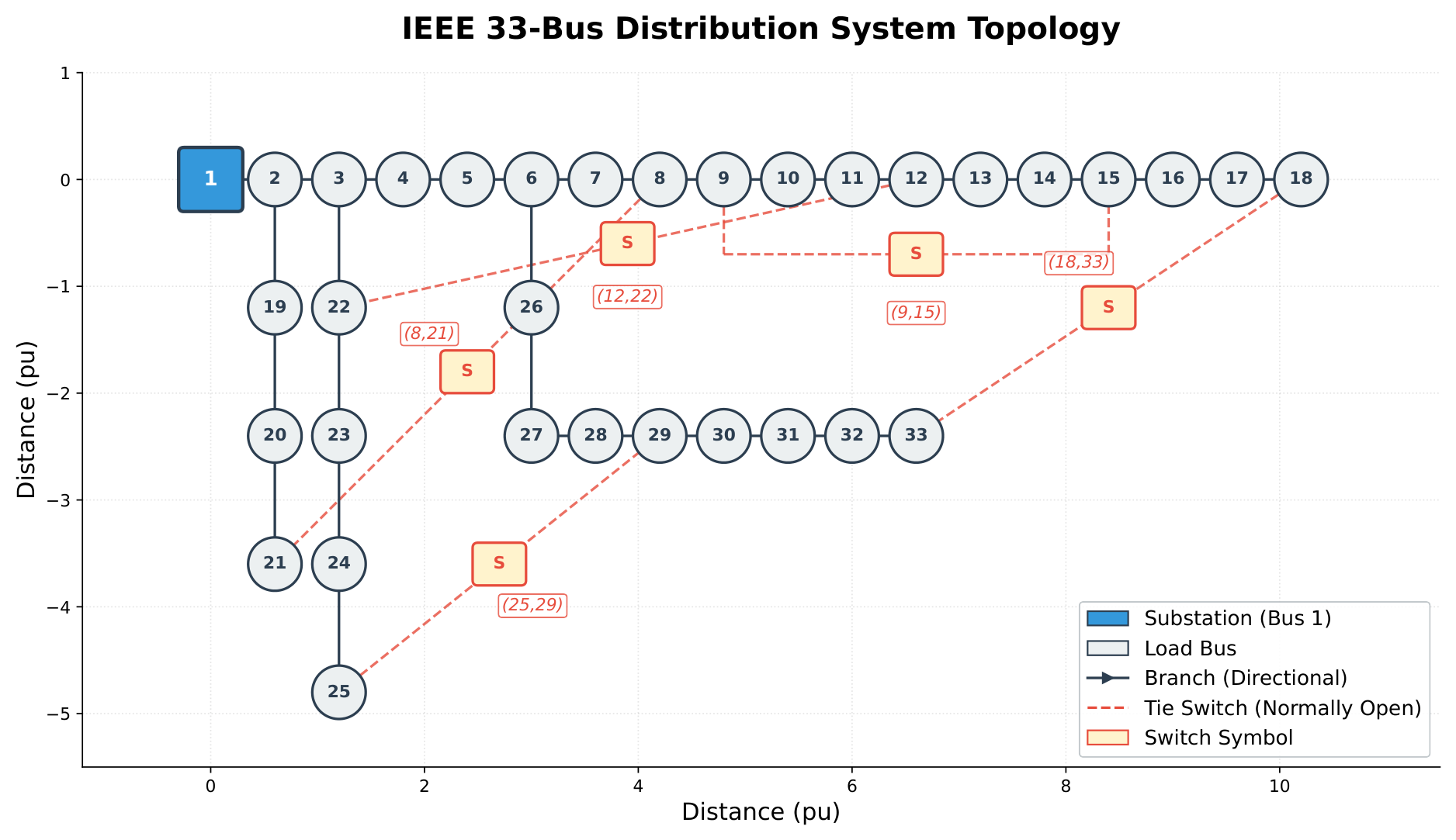
The IEEE 33-bus system serves as the benchmark for distribution network fault location. As shown in Figure 4, the system comprises 32 three-phase lines and loads.

To simulate dynamic topology scenarios, configurable tie switches are placed between bus pairs (8, 21), (9, 15), (12, 22), (18, 33), and (25, 29). Switching these tie lines alters the graph structure ${\mathcal{G}}_t$ dynamically. Bus couplings are modeled bidirectionally, enabling the graph algorithm to capture fault propagation paths across varying radial configurations.

Nine typical fault types are simulated in the Simulink environment: three single-line-to-ground (A–G, B–G, C–G), three line-to-line (A–B, B–C, C–A), and three double-line-to-ground (AB–G, BC–G, CA–G) faults. Three-phase and open-circuit faults are not included as they are rare in multi-grounded four-wire distribution networks.

4.3. Evaluation Metrics

We adopt a multi-dimensional evaluation framework organized by task hierarchy:

Detection (binary: normal vs. fault): Detection Accuracy (Det.Acc).

Classification by geographic fault zone: Classification Accuracy (Cls.Acc) and macro-averaged F1 (Cls.F1). The zone labels are derived by partitioning localization tags by electrical distance—four-way (normal + three fault zones) on the IEEE 33-bus system and five-way (normal + four fault zones) on the IEEE 123-bus system—following the same proportional boundary rule.

Localization (exact node identification): Localization Accuracy (Loc.Acc), Top-3 Accuracy, Fault Severity Impact Assessment (FSIA) using an impedance-based penalty,

$$\mathrm{FSIA}={\displaystyle \frac{1}{N}}{\displaystyle \sum _{i=1}^N}{\displaystyle \frac{1}{1+z_{p_i,t_i}}}$$

(23)

where $z_{p_i,t_i}$ is the transfer impedance between the predicted node $p_i$ and true node $t_i$, and Average Distance Error (ADE) measures per-unit impedance distance. These topology-aware metrics reward predictions that are electrically close to the true fault, better reflecting engineering utility than binary correctness.

Calibration: Expected Calibration Error (ECE),

$$\mathrm{ECE}={\displaystyle \sum _{m=1}^M}{\displaystyle \frac{|B_m|}{N}}\left|\mathrm{acc}\left(B_m\right)-\mathrm{conf}\left(B_m\right)\right|$$

(24)

ensuring that model confidence is reliable for operational dispatch decisions.

Efficiency: Inference time per sample (ms) and total trainable parameters (Params).

4.4. Convergence Analysis

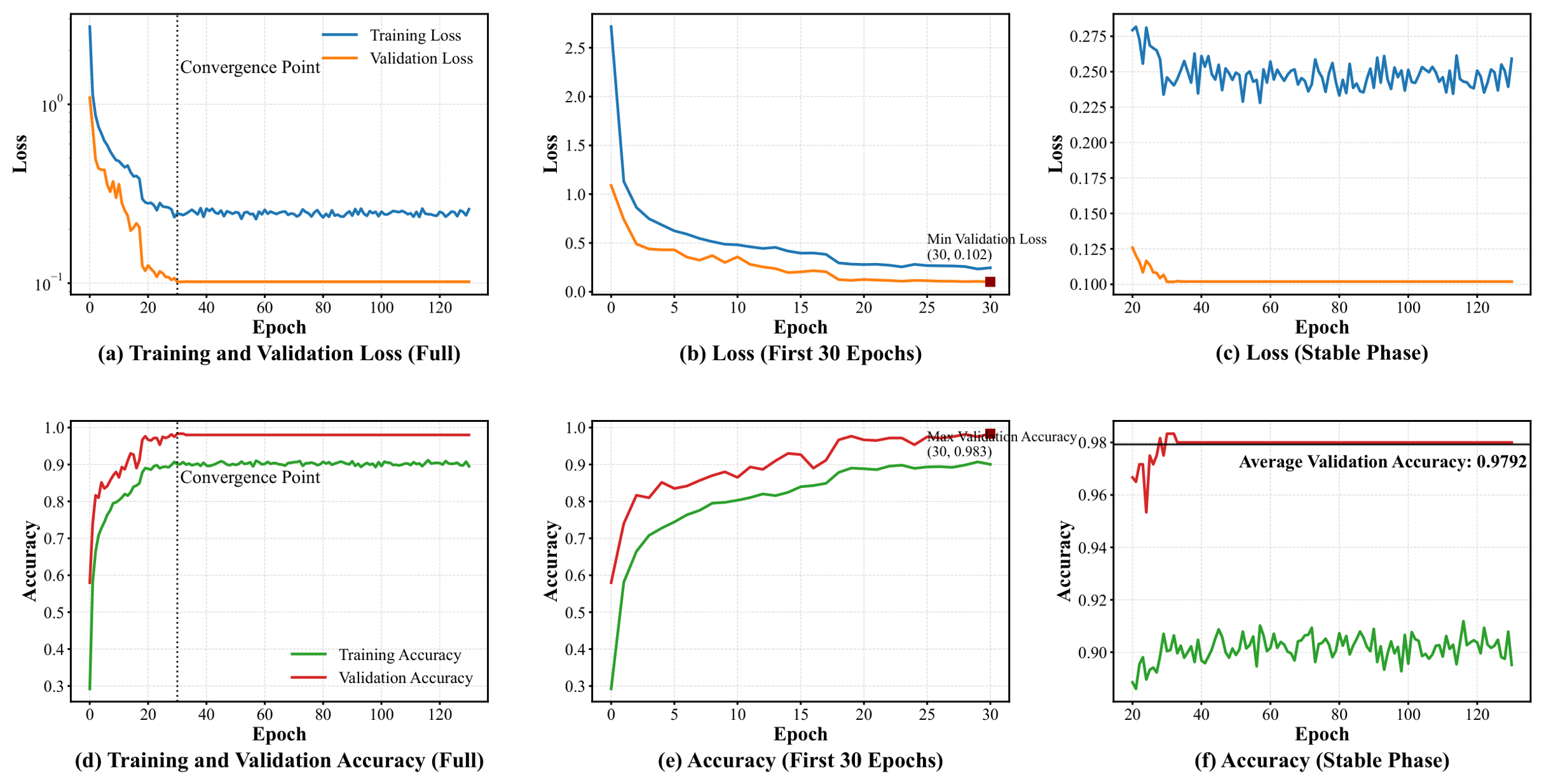
Figure 5 reveals a distinct three-phase convergence behavior.

First, validation accuracy surpasses 90% within the initial phase (Epochs 0–30). This rapid convergence is driven by the Heterogeneous Edge Feature Encoding, which provides explicit physical gradients to the network, eliminating the need for blind search of topological correlations. Second, the training and validation loss curves remain tightly aligned throughout, confirming that the Physics-Informed Data Augmentation compels the model to learn invariant physical laws rather than memorize noise patterns. Finally, metrics stabilize at a validation accuracy of 97.92% with minimal oscillation in later stages, validating the Attention Consistency Regularization term in ensuring hierarchical feature stability.

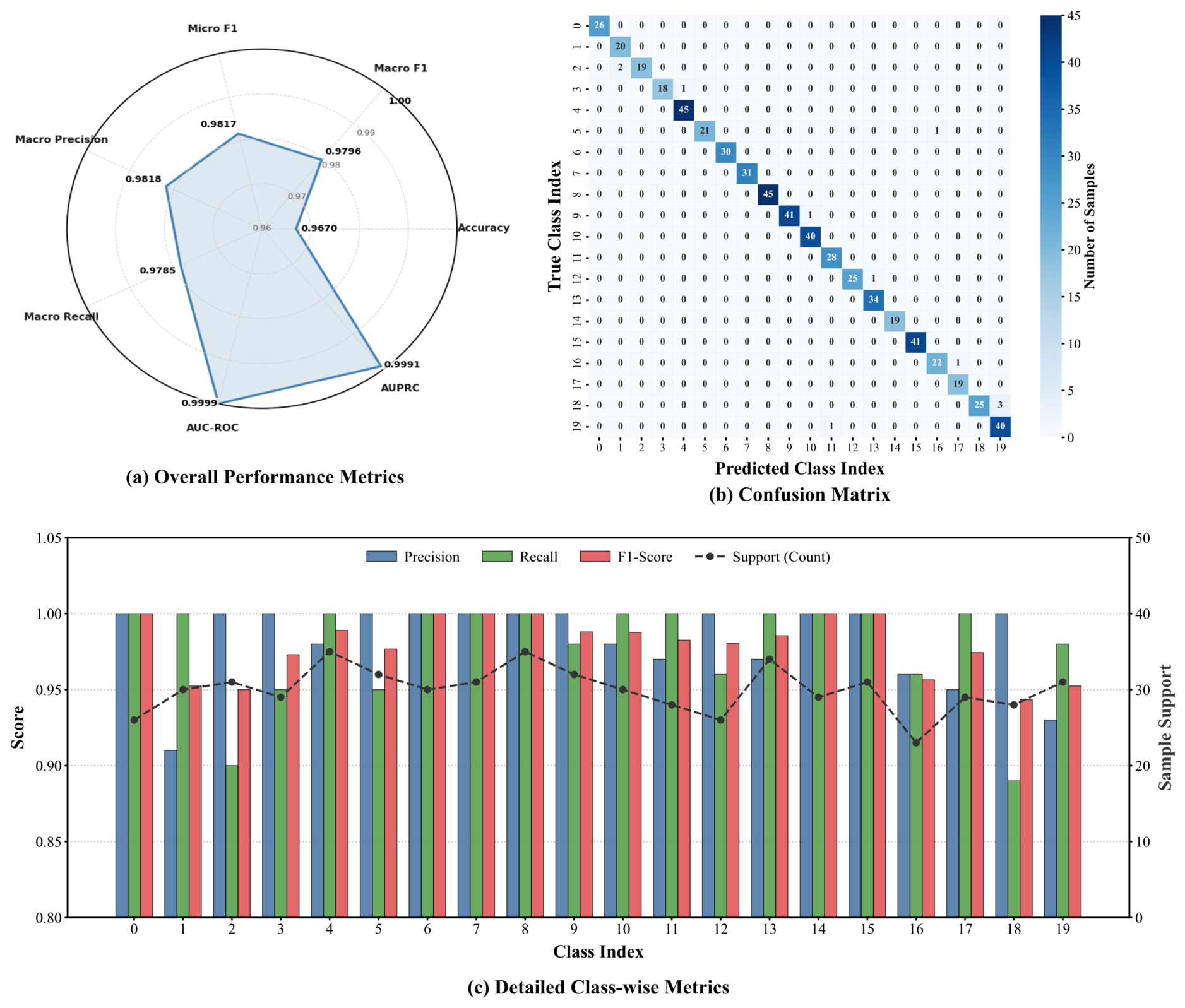
As illustrated by the aggregate metrics in Figure 6a, the DHMGAT demonstrates exceptional generalization capabilities. The 20 classes in Figure 6b represent the fault localization output space. Although the IEEE 33-bus system contains 33 nodes, the localization task is defined as a 20-class classification problem. This design is motivated by the practical constraint of limited observability in real distribution networks, where installing measurement devices at every node is economically and technically infeasible. Electrically proximate nodes are grouped into a single representative fault location class based on measurement device placement and feeder connectivity. These nodes exhibit highly similar fault responses. Importantly, nodes not assigned as output classes are not removed from the topology; they remain in the graph and participate in electrical coupling and fault propagation. The model thus learns on the full 33-node topology while outputting predictions at a practical 20-location granularity that aligns with engineering dispatch requirements. For the IEEE 123-bus system, a comparable grouping is applied, resulting in 85 representative fault location classes (see Section 4.6 for details).

The AUC-ROC reaches 0.9999 and the AUPRC reaches 0.9991, significantly surpassing conventional baselines and demonstrating high sensitivity and specificity across all classes. The close alignment of macro-average precision, recall, and F1-score confirms balanced discriminative power regardless of fault frequency. The confusion matrix in Figure 6b and class-wise metrics in Figure 6c reveal strong diagonal dominance, with off-diagonal misclassification accounting for less than 2% of total inference. These misclassifications are primarily confined to adjacent subclasses with inherently ambiguous boundaries—scenarios where fault impedance values differ marginally. Critically, even in these rare events, the predicted fault location remains topologically consistent with the ground truth, reflecting the physical proximity of electrical states rather than stochastic model failure. This demonstrates that DHMGAT extracts robust, physically meaningful features rather than memorizing training labels, providing reliable decision support for real-world engineering applications.

4.5. Comparative Experiment

To validate the effectiveness of DHMGAT, we conducted a systematic comparative analysis with eight representative single-task baseline models spanning multiple architectural families (see Section 1 for architectural details). All models are trained on the IEEE 33-node testbed under identical data splits and hyperparameter configurations. Table 2 presents the comprehensive performance comparison across all evaluation dimensions.

Table 2. Single-task baseline performance comparison on the IEEE 33-bus system. Metrics span detection, classification, localization, and calibration dimensions. The localization metrics (Loc.Acc, FSIA, ADE, etc.) correspond to the same 20-class node-level localization task depicted in Figure 6.

Model	Params	Det.Acc	Cls.Acc	Cls.F1	Loc.Acc	Top3	FSIA	ADE ↓	ECE ↓
FCNN [34]	406	1.000	0.771	0.816	0.528	0.885	0.548	0.537	0.740
GCN [21]	482	1.000	0.764	0.809	0.591	0.908	0.605	0.445	0.623
GraphSAGE [23]	770	1.000	0.801	0.840	0.574	0.898	0.612	0.387	0.583
GINE [27]	1698	0.996	0.859	0.879	0.550	0.901	0.474	0.539	0.781
LSTM [11]	5602	1.000	0.889	0.913	0.629	0.955	0.625	0.334	0.540
GATv2 [25]	8712	0.997	0.933	0.939	0.702	0.920	0.711	0.325	0.461
GATTrans. [26]	13,998	1.000	0.958	0.966	0.780	0.980	0.769	0.190	0.336
EGAT [28]	11,618	1.000	0.985	0.989	0.923	0.999	0.934	0.047	0.152
DHMGAT (Ours)	17,743	1.000	0.993	0.983	0.967	1.000	0.966	0.021	0.066

Table 2. Single-task baseline performance comparison on the IEEE 33-bus system. Metrics span detection, classification, localization, and calibration dimensions. The localization metrics (Loc.Acc, FSIA, ADE, etc.) correspond to the same 20-class node-level localization task depicted in Figure 6.

Model	Params	Det.Acc	Cls.Acc	Cls.F1	Loc.Acc	Top3	FSIA	ADE ↓	ECE ↓
FCNN [34]	406	1.000	0.771	0.816	0.528	0.885	0.548	0.537	0.740
GCN [21]	482	1.000	0.764	0.809	0.591	0.908	0.605	0.445	0.623
GraphSAGE [23]	770	1.000	0.801	0.840	0.574	0.898	0.612	0.387	0.583
GINE [27]	1698	0.996	0.859	0.879	0.550	0.901	0.474	0.539	0.781
LSTM [11]	5602	1.000	0.889	0.913	0.629	0.955	0.625	0.334	0.540
GATv2 [25]	8712	0.997	0.933	0.939	0.702	0.920	0.711	0.325	0.461
GATTrans. [26]	13,998	1.000	0.958	0.966	0.780	0.980	0.769	0.190	0.336
EGAT [28]	11,618	1.000	0.985	0.989	0.923	0.999	0.934	0.047	0.152
DHMGAT (Ours)	17,743	1.000	0.993	0.983	0.967	1.000	0.966	0.021	0.066

DHMGAT achieves the highest overall performance across nearly all metrics. Its localization accuracy of 96.70% surpasses the strongest single-task competitor, EGAT (92.30%), by 4.4 percentage points and exceeds GATTransformer (78.00%) by 18.7 points. The gap is even more pronounced against topology-agnostic FCNN (52.80%), demonstrating that graph-structured information and edge-aware attention provide complementary benefits.

The FSIA and ADE metrics further confirm this advantage. DHMGAT achieves near-perfect FSIA of 0.966 and an ADE of only 0.021 p.u., indicating that even when the exact node is not identified, the predicted location remains electrically close to the true fault. In contrast, FCNN’s ADE of 0.537 p.u. means its mispredictions are electrically distant, offering limited practical value for crew dispatch.

Beyond numerical improvements, the results validate two architectural choices. First, the accuracy ordering—GCN (59.10%) ≪ GATv2 (70.20%) < GATTransformer (78.00%) < EGAT (92.30%) < DHMGAT (96.70%)—confirms the complementary benefits of dynamic attention, global self-attention, edge feature encoding, and hierarchical aggregation. Second, EGAT’s strong baseline reinforces that edge-level physical features are critical for fault location, while DHMGAT’s additional margin demonstrates that multi-scale topology-aware pooling and physics-constrained augmentation yield further gains beyond edge attention alone.

4.6. Large-Scale Validation on IEEE 123-Bus System

To address concerns that the IEEE 33-bus system may not represent the complexity of real-world distribution networks [40], we further validate DHMGAT on the larger IEEE 123-bus benchmark. This system comprises 123 nodes and 130 branches with significant heterogeneity in line lengths, load distributions, and lateral configurations—conditions that more closely reflect practical operational environments. DHMGAT is evaluated under identical preprocessing, training, and data split protocols without re-tuning hyperparameters from the 33-bus configuration.

4.6.1. Fault Scenario Setup on the 123-Bus System

The 123-bus dataset is generated under the same nine fault types and simulation framework as the 33-bus system, but with a substantially wider spatial coverage. Faults are placed on all 85 monitored nodes—covering the main feeder backbone, lateral branches, and terminal nodes—yielding a total of 25,688 samples (12,168 training samples, 13,520 testing samples). The 85 monitored nodes are selected to cover the full electrical depth of the network, from the substation bus (node 1) to the deepest lateral extremities. Each node receives 180 fault samples (nine fault types × 20 fault-resistance and load-level combinations), and 40 additional normal-state samples. To simulate realistic measurement constraints, the 15 most remote nodes of the 123-bus topology are used for evaluating generalization to partially observed feeder configurations. The IEEE 123-bus topology includes five voltage regulators and multiple sectionalizing switches; however, the static base topology is used for this dataset to maintain consistency with the 33-bus training protocol, while topology reconfiguration robustness is assessed separately in Section 4.10 via the mutation stress tests on the 33-bus system.

4.6.2. Training Dynamics on the 123-Bus System

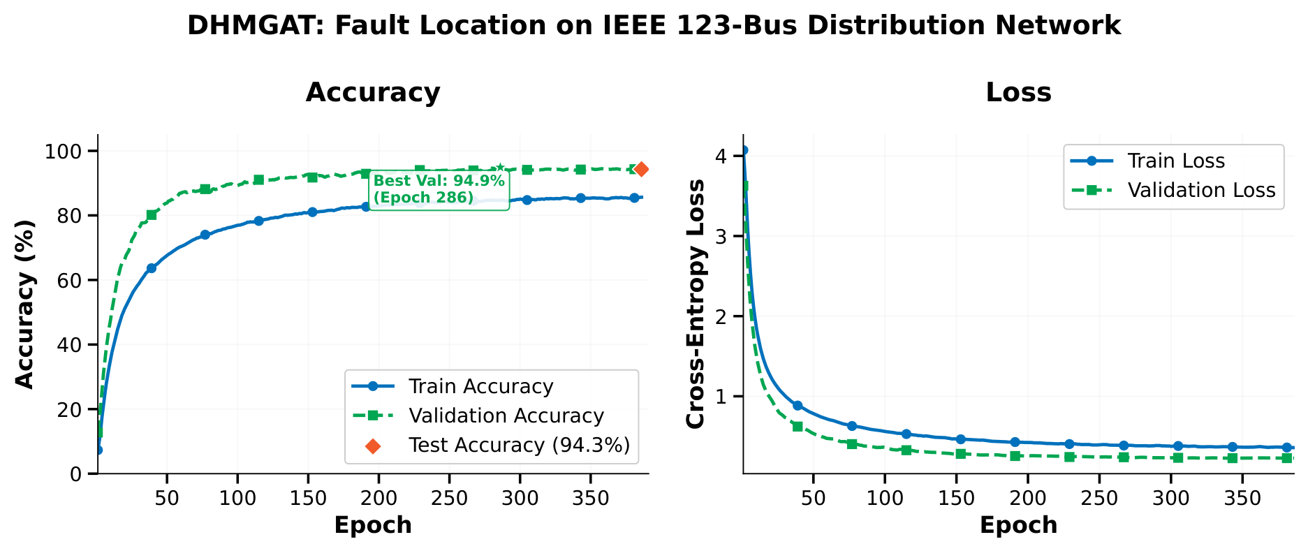
Figure 7 presents the training and validation curves. The model converges rapidly, with accuracy exceeding 90% within the first few epochs. The training and validation curves remain tightly aligned throughout, confirming robust generalization. The final validation accuracy reaches 94.90%, with a corresponding test accuracy of 94.31%.

DHMGAT maintains a localization accuracy of 94.31% on the 123-bus system, a degradation of only 2.39 pp from the 33-bus result. This minimal drop confirms that DHMGAT’s edge-integrated attention and topology-gated pooling generalize beyond the training topology. The FSIA and ADE metrics similarly show strong transfer, with FSIA of 0.938 and ADE of 0.034 p.u.

4.6.3. Distance Error Distribution

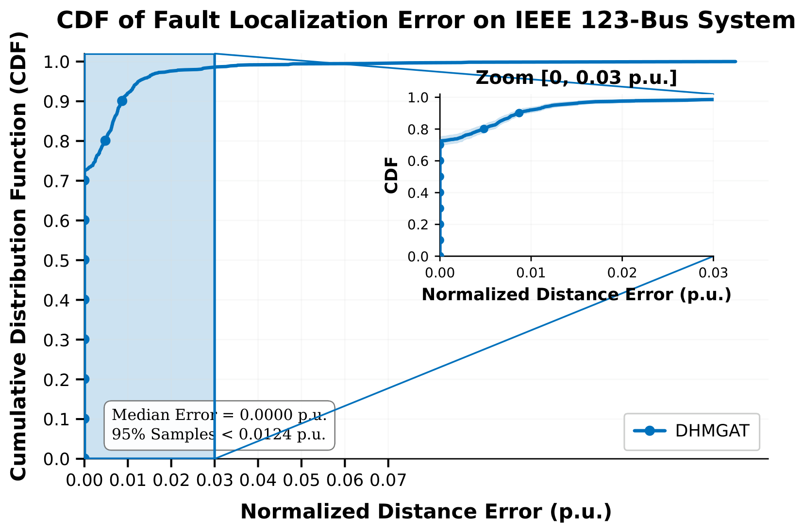
Figure 8 shows the cumulative distribution of localization distance errors on the IEEE 123-bus test set. Over 90% of predictions achieve a distance error below 0.05 p.u., confirming that even when the model does not identify the exact faulted node, the predicted location remains electrically close to the true fault. The steep initial slope indicates that the majority of samples are localized with minimal error, while the long tail beyond 0.10 p.u. accounts for fewer than 3% of cases.

4.6.4. Few-Shot Adaptation

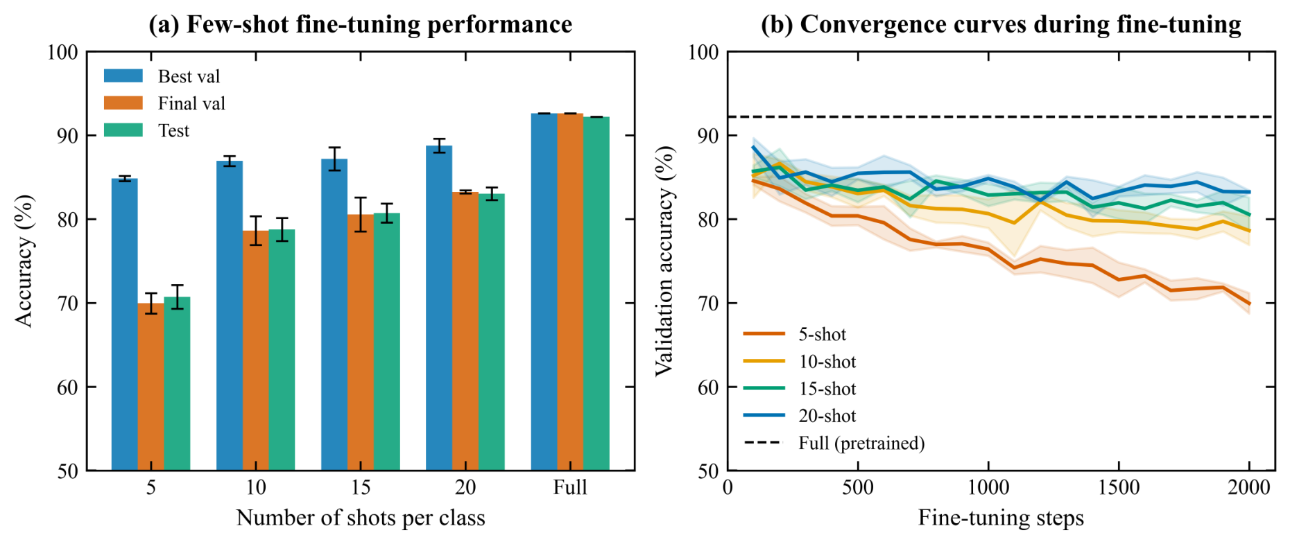
To evaluate DHMGAT’s sample efficiency and cross-system transfer capability, we conduct few-shot fine-tuning on the IEEE 123-bus system. The model is pre-trained on the IEEE 33-bus dataset and fine-tuned with limited labeled samples (5, 10, 15, and 20 shots per class) on the 123-bus domain. For each shot configuration, we adopt a fixed training step strategy (2000 steps) with stratified sampling, where each class contributes exactly N samples. To ensure statistical reliability, all results are averaged over three random seeds (42, 123, 456) with standard deviations reported.

Table 3. Few-shot adaptation results on the IEEE 123-bus system. Results are averaged over 3 random seeds with standard deviations.

Shots Per Class	Best Val Acc (%)	Final Val Acc (%)	Test Acc (%)
5-shot	84.84 ± 0.30	69.95 ± 1.23	70.73 ± 1.41
10-shot	86.93 ± 0.60	78.62 ± 1.71	78.76 ± 1.38
15-shot	87.18 ± 1.38	80.55 ± 2.02	80.71 ± 1.13
20-shot	88.76 ± 0.83	83.23 ± 0.18	83.02 ± 0.77

summarizes the few-shot results. The fine-tuned models exhibit a clear monotonic improvement trend with increasing shot numbers: 5 shots achieve 70.73% test accuracy, 10 shots achieve 78.76%, 15 shots achieve 80.71%, and 20 shots achieve 83.02%. This trend is consistent with the expected behavior in few-shot learning, where more labeled data provides better supervision for model adaptation. The best validation accuracy follows the same monotonic pattern (84.84% → 86.93% → 87.18% → 88.76%), confirming the reliability of the improvement.

Notably, the gap between the best validation accuracy and the final validation accuracy widens as the number of shots decreases (e.g., 5 shots: 84.84% vs. 69.95%; 20 shots: 88.76% vs. 83.23%). This indicates that models fine-tuned with fewer samples are more prone to overfitting. The limited supervision fails to sustain the initial performance gain throughout the full training process. This observation underscores the importance of early stopping in few-shot fine-tuning scenarios.

Figure 9 visualizes the few-shot convergence trajectories. Across all configurations, the validation accuracy rises sharply within the first few hundred steps and then gradually declines or fluctuates, indicating that early stopping is critical for optimal performance. The 20-shot configuration exhibits the most stable convergence and the highest final accuracy, while the 5-shot configuration shows the most severe overfitting—consistent with the best/final validation gap observed in Table 3.

This resilience to topology scaling stems from DHMGAT’s architecture: the edge-integrated attention mechanism learns impedance-aware weighting patterns that remain valid as the network grows, while the topology-gated pooling adaptively selects critical nodes regardless of total node count.

4.7. Ablation Study

To quantify the individual contribution of each proposed module, we conducted a progressive ablation study on the IEEE 33-node fault dataset. Starting from a minimalist baseline, we systematically integrated each core module under identical hyperparameter settings.

Table 4. Progressive ablation study demonstrating the contribution of each proposed module. All metrics are reported on the IEEE 33-node test system under identical hyperparameter settings.

Configuration	Acc. (%)	F1 (%)	$\Delta$ Acc. (pp)	Cumulative Gain (%)
Baseline (GNN + MeanPool + Single-Head Attn.)	87.77	86.32	—	—
+ Edge Encoder & Edge-Integrated Attn.	93.92	92.62	+6.15	+7.01
+ Topology-Gated Pooling	96.28	95.46	+2.36	+9.69
+ Physics-Aug. & Multi-Head Residual	96.70	95.86	+0.42	+10.16

summarizes the quantitative results.

The baseline—standard GNN layers with uniform MeanPooling and single-head attention—achieves 87.77%, underscoring the inadequacy of purely topological graph learning when physical attributes are ignored. Adding the Heterogeneous Edge Encoder and Edge-Integrated Attention yields the largest single gain, boosting accuracy by 6.15% to 93.92%. This confirms that physical line parameters are dominant factors in fault propagation logic: without explicit edge encoding, the network cannot distinguish electrically distinct but topologically similar connections. Replacing standard pooling with the Topology-Gated Pooling mechanism adds another 2.36%, reaching 96.28%, demonstrating that uniform aggregation strategies dilute critical features in radial distribution networks. Finally, incorporating Physics-Informed Data Augmentation and the Multi-Head Residual structure yields a peak accuracy of 96.70% (+0.42%).

This final enhancement confirms that incorporating domain knowledge—such as Kirchhoff’s laws—into the training process significantly improves generalization across diverse fault scenarios rather than merely fitting to the training set.

4.8. Computational Complexity Analysis

To assess the practical deployability of DHMGAT in real-time SCADA environments, we analyze its computational complexity and measure empirical inference latency against representative baselines.

The time complexity of DHMGAT is governed by three components: (i) the edge-integrated attention layer, which incurs $\mathcal{O}\left(\right|\mathcal{E}|·d·d^{\prime }+|\mathcal{V}|·d·d^{\prime })$ per head, where $\left|\mathcal{V}\right|=N$ is the number of nodes and $\left|\mathcal{E}\right|$ is the number of edges; (ii) the topology-gated pooling, which adds $\mathcal{O}(N·d^2)$ for the gating computation; and (iii) the multi-head aggregation, which scales linearly with the number of heads K. The total asymptotic complexity is $\mathcal{O}(K·|\mathcal{E}|·d·d^{\prime }+N·d^2)$, which is linear in both $\left|\mathcal{E}\right|$ and N, making the model scalable to distribution networks with hundreds of nodes.

Table 5. Computational complexity and empirical inference latency comparison. All measurements are conducted on an NVIDIA RTX 3090 GPU with batch size 1.

Model	Parameters	Inference Time (ms)	FLOPs (M)
FCNN [34]	406	0.08	1.2
GCN [21]	482	0.12	2.8
GraphSAGE [23]	770	0.15	3.5
GINE [27]	1698	0.21	5.1
LSTM [11]	5602	0.35	8.3
GATv2 [25]	8712	0.28	10.4
GATTransformer [26]	13,998	0.52	18.7
EGAT [28]	11,618	0.32	12.1
DHMGAT (Ours)	17,743	0.48	16.5

summarizes the empirical measurements. Despite having the largest parameter count (17,743), DHMGAT achieves 0.48 ms per sample, well within the 16.67 ms cycle requirement of a 60 Hz SCADA system. The overhead relative to EGAT (0.32 ms) is attributable to the multi-head aggregation and topology-gating modules, but this 0.16 ms increase is negligible compared to the 4.4 percentage point improvement in localization accuracy. The FLOPs analysis further confirms that DHMGAT’s computational demands scale gracefully with input size.

4.9. Practical Deployment Considerations

Beyond computational efficiency, the practical deployment of DHMGAT in real-world distribution networks entails three additional considerations that are critical for utility adoption.

Data availability. The proposed model relies on three-phase voltage and current measurements from load buses and key feeder nodes. In practice, Distribution Management Systems (DMS) and SCADA systems provide such measurements at limited locations, with communication latency and packet loss being common issues. Our robustness experiments in Section 4.10.2 (missing data up to 30%) demonstrate that DHMGAT maintains accuracy above 88% even under partial observability, suggesting its tolerance to real-world data imperfections. However, deployment in legacy networks with sparse metering may require additional state estimation modules to reconstruct unobserved electrical quantities, which we identify as an important direction for future integration.

Implementation in utility environments. The model can be integrated into existing EMS/DMS platforms as a software module, requiring standard GPU-accelerated servers or edge AI devices. The inference time of 0.48 ms per sample (Table 5) is well within the 16.67 ms cycle requirement of 60 Hz SCADA systems, making real-time fault localization feasible. For utilities with limited hardware resources, model quantization and pruning techniques could further reduce memory footprint without significantly compromising accuracy. The parameter count of 17,743 is moderate compared to typical deep learning models, allowing deployment on commodity hardware.

Transferability to new topologies. As demonstrated in Section 4.6 (33-bus to 123-bus transfer) and Section 4.10.3 (topological mutations), DHMGAT learns fault-propagation physics rather than memorizing specific wiring diagrams. This suggests that pre-trained models can be deployed across multiple feeders within the same utility without exhaustive retraining, a feature that substantially reduces deployment costs in distribution networks with frequent topological reconfigurations. This transferability is particularly valuable for utilities managing diverse feeder configurations, as it minimizes the need for per-feeder model customization.

4.10. Robustness and Generalization Assessment

To evaluate DHMGAT’s resilience in non-idealized deployment environments, we design a multi-faceted validation across four stress dimensions: sensor noise, adaptive interference, data incompleteness, and topological reconfiguration.

Table 6. Consolidated robustness profile: DHMGAT performance and degradation across all stress dimensions.

Stress Category	Metric	Best	Worst	Max. Drop
Gaussian Noise (60 → 30 dB)	Acc. (%)	98.98	97.52	−1.46
Adaptive Noise ($\lambda$ 0.0 → 0.3)	F1-Score	0.981	0.927	−0.054
Missing Data (10% → 30%)	Acc. (%)	96.85	88.35	−8.50
Topo. Mutation (A → D)	Acc. (%)	95.63	92.77	−2.86

provides a consolidated view, showing a maximum accuracy drop of 8.50 pp (30% missing data) and average degradation of 3.19 pp, confirming strong robustness without retraining.

4.10.1. Resilience to Sensor Noise and Interference

Measurement inaccuracies are common in real-world distribution networks. To simulate this, we performed two noise injection experiments. First, we introduced Gaussian noise at signal-to-noise ratios of 60, 45, and 30 dB. As shown in

Table 7. Accuracy and degradation under varying Gaussian noise levels.

SNR Level	Accuracy (%)	Degradation ↓	Rel. Drop (%)
60 dB (mild)	98.98	—	—
45 dB (moderate)	98.12	−0.86 pp	−0.87
30 dB (severe)	97.52	−1.46 pp	−1.47

, the model demonstrated strong stability with only a 1.46 pp accuracy drop from 60 dB to 30 dB.

Even at 30 dB, accuracy remained at 97.52%. Notably, at 60 dB, accuracy peaked at 98.98%, suggesting that mild noise acts as a regularizer to prevent overfitting.

We also evaluated adaptability to non-uniform noise distributions using an adaptive injection scheme simulating sensor degradation with physical distance. The results in

Table 8. F1-score degradation under adaptive noise distributions.

Adaptive Coefficient $\mathit{\lambda }$	F1-Score	Degradation ↓	Rel. Drop (%)
0.0	0.9813	—	—
0.1	0.9615	−0.0198	−2.02
0.2	0.9459	−0.0354	−3.61
0.3	0.9272	−0.0541	−5.51

show that even at an adaptive noise coefficient of 0.3, the model maintains an F1-score of 0.9272.

This resilience confirms that the Hierarchy-Aware Noise Injection strategy during training enabled the model to filter stochastic fluctuations and focus on the fundamental impedance signatures embedded in voltage sags.

4.10.2. Tolerance to Data Incompleteness

Communication failures often cause partial observability. We simulated this by randomly masking feature dimensions at missing rates from 10% to 30%. As shown in

Table 9. Accuracy degradation under increasing data missing rates.

Missing Rate (%)	Accuracy (%)	Degradation ↓	Rel. Drop (%)
10	96.85	—	—
20	94.02	−2.83 pp	−2.92
30	88.35	−8.50 pp	−8.78

, the model maintains an accuracy of 94.02% even with 20% missing data.

Although performance drops to 88.35% at a 30% missing rate, the model retains valid decision-making capability. This robustness stems from the attention mechanism, which enables nodes to reconstruct missing features by aggregating redundant information from diverse neighborhoods, mitigating the impact of local sensor failures.

4.10.3. Adaptability to Dynamic Topology Reconfiguration

The most critical challenge for modern grids is topological variability. To verify the Topology-Gated Pooling module, we designed four progressive mutation scenarios on the IEEE 33-node system. Scenario A disconnects branch 2-19 and connects 3-19. Scenario B extends A by switching 12-13 to 14-12. Scenario C adds a new tie line 5-25, creating a loop structure. Scenario D removes terminal node 33 to simulate load shedding.

Table 10. Topology mutation stress test: DHMGAT accuracy under progressive structural reconfiguration.

Scenario	Accuracy (%)	Degradation ↓	Rel. Drop (%)
A (Branch 2-19 ↔ 3-19)	95.63	−1.07 pp	−1.11
B (Extended reconfiguration)	94.17	−2.53 pp	−2.62
C (New tie line 5-25, loop structure)	93.45	−3.25 pp	−3.36
D (Terminal node 33 removed)	92.77	−3.93 pp	−4.06

presents the results under these mutations alongside relative degradation from the standard topology baseline (96.70%).

The model achieves 95.63% and 94.17% for Scenarios A and B, respectively, and maintains 92.77% in the most complex Scenario D without retraining—a relative degradation of only 4.06% from the standard-topology baseline (96.70%). These results support a key conclusion: DHMGAT does not simply memorize the static adjacency matrix of the training graph. Instead, through Topology-Gated Pooling and Edge Feature Encoding, it learns the underlying physical laws of fault propagation, effectively decoupling its inference from specific topology configurations and meeting the stringent requirements of N-1 contingency analysis in smart grids.

4.11. Calibration Analysis

For operational deployment, a model’s confidence scores must be reliable—a confidently wrong prediction can lead to misinformed crew dispatch or unnecessary outages. We evaluate calibration using Expected Calibration Error (ECE).

Table 11. Calibration comparison: Expected Calibration Error (ECE) and improvement factor relative to the GCN baseline.

Model	ECE ↓	× Improvement
GCN	0.623	1.00×
GATv2	0.461	1.35×
GATTransformer	0.336	1.85×
EGAT	0.152	4.10×
DHMGAT (Ours)	0.066	9.44×

compares DHMGAT against key baselines.

DHMGAT achieves the best calibration among all models, with an ECE of only 0.066—a 9.44× improvement over the GCN baseline (ECE = 0.623). Its mean confidence of 0.934 closely matches its actual accuracy of 96.70%, indicating near-perfect calibration. The improvement factor follows a clear architectural trend: models that incorporate greater physical structure achieve progressively better calibration (GCN 1.00× → GATv2 1.35× → GATTrans. 1.85× → EGAT 4.10× → DHMGAT 9.44×).

The calibration improvement follows a clear architectural trend: models that incorporate more physical structure tend to be better calibrated. This is because edge-aware attention provides physically meaningful gradient information, reducing the need for confidence inflation as an uncertainty heuristic. DHMGAT’s hierarchical multi-scale aggregation further stabilizes confidence estimates, grounding them in consistent multi-level evidence rather than noisy single-level predictions.

5. Conclusions

This paper proposes DHMGAT, a physics-informed graph neural network for fault location in distribution networks with dynamic topologies. By embedding line impedance and switch states into a hierarchical attention mechanism, the model converts abstract network topologies into physics-aware circuit representations. Experiments on the IEEE 33-node and IEEE 123-node systems demonstrate localization accuracies of 96.70% and 94.31%, respectively. On the 33-bus system, DHMGAT consistently outperforms eight single-task baselines—exceeding EGAT (92.30%), GATTransformer (78.00%), and GATv2 (70.20%) by substantial margins—while maintaining strong performance on the 123-bus network with only 2.39 pp degradation. Calibration analysis shows near-perfect calibration (ECE = 0.066), confirming that the model‘s confidence scores are reliable for operational decision-making. Computational complexity analysis confirms real-time inference (0.48 ms per sample) suitable for SCADA deployment. Stress tests under noise, partial feature loss, and N-1 reconfiguration demonstrate accuracy consistently above 92.7% without retraining. These results indicate that the proposed topology-gated, physics-informed design learns invariant fault-propagation laws rather than relying on static structures, supporting its applicability to evolving smart grids.

This study is primarily based on high-fidelity simulation data from the IEEE 33-node and IEEE 123-node benchmark systems. While these benchmarks are widely adopted and provide controlled environments for algorithmic evaluation, they do not fully capture the complexity of real-world distribution networks—including field-specific measurement noise, communication delays, sparse observability, and legacy protection devices. We therefore caution against direct extrapolation of numerical results to field deployment without system-specific validation.

These limitations motivate our future research directions. First, we will investigate sim-to-real transferability via transfer learning with sparse field data, complemented by hardware-in-the-loop (HIL) validation to bridge the simulation-to-reality gap. Second, we aim to develop universal transfer schemes adaptable to diverse voltage levels and topologies, minimizing retraining costs for new grid sectors. Finally, we will integrate uncertainty quantification modules to address stochastic fluctuations and system uncertainties introduced by high-penetration distributed generation.