Study on the Non-Equilibrium Dynamic Phase Transition Model for Oil–Gas Systems

Abstract

In gas-condensate reservoirs, the phase behavior of reservoir fluids is inherently dynamic during pressure depletion. When the rate of external pressure decline exceeds the intrinsic relaxation rate governing phase equilibrium, the system deviates from thermodynamic equilibrium and exhibits pronounced non-equilibrium effects. These transient behaviors significantly influence fluid properties; meanwhile, conventional equilibrium models neglect phase transition lag, resulting in inaccurate phase behavior and biased production predictions. In this study, a non-equilibrium dynamic phase transition model is developed to quantitatively couple the pressure depletion rate with the relaxation kinetics of the system. This model, established based on controlled non-equilibrium phase transition experiments performed on the condensate-gas fluid investigated in this work, provides an analytical framework for describing the temporal evolution of phase behavior under dynamic conditions. Model validation through integrated experimental measurements and numerical simulations shows good agreement between calculated and measured results for the studied condensate-gas system, with average relative errors below 5%. Results reveal that accelerated pressure depletion strengthens non-equilibrium effects. At a rate of 15 MPa/h, the relative volume and retrograde condensate saturation decrease by 9.09% and 5.38%, respectively, while condensate recovery improves by 13.85%. Moreover, the characteristic relaxation time toward equilibrium exhibits a strong dependence on the depletion rate, increasing as the depletion rate rises. This work provides an experimentally constrained analytical framework for describing rate-dependent non-equilibrium phase behavior during pressure depletion and for interpreting its impact on condensate recovery in the specific condensate-gas system studied. Although the governing framework may be transferable to other rate-sensitive hydrocarbon systems after fluid-specific recalibration, the parameterized analytical model and validation presented in this study are limited to the investigated condensate-gas fluid, and its applicability to other hydrocarbon fluid types remains to be evaluated in future studies.

1. Introduction

In oil–gas systems, phase transitions frequently occur under dynamic and non-equilibrium conditions rather than strictly at thermodynamic equilibrium. Equilibrium phase transitions are relative thermodynamic phenomena that assume sufficient time for the system to stabilize, whereas non-equilibrium transitions are absolute kinetic processes constrained by the composition between external perturbations and intrinsic phase transition rates. In condensate gas and volatile oil reservoirs under depletion, when the rate of external pressure change exceeds the intrinsic phase transition rate, the system is unable to reach equilibrium instantaneously, and a pronounced lag in phase behavior emerges. This lag is typically reflected as deviations in fundamental phase parameters—such as saturation (S), volume (V), and condensate recovery factor (η)—from their corresponding equilibrium values, and indicates that the system requires a characteristic relaxation time to reach a new equilibrium state. Such deviations become particularly evident during the depletion of condensate-gas and volatile oil reservoirs, or in gas injection flooding processes, where the emergence of a second fluid phase amplifies non-equilibrium effects [1,2].

Given the substantial influence of non-equilibrium phase transitions on the dynamics of oil and gas production, extensive efforts have been made to investigate these effects in both laboratory and field operations [3,4]. In condensate-gas reservoirs, Mirzazhanzade et al. [5] found through core depletion experiments that the system does not reach thermodynamic equilibrium, and that condensate saturation is strongly governed by the rate of pressure depletion. Saeidi et al. [6] further confirmed, using pressure depletion experiments at varying rates, that faster depletion rates lead to more pronounced non-equilibrium effects. Consistent findings were reported by Guo et al. [7,8], Sui et al. [9], and Xie et al. [10], who performed long-core depletion experiments and showed that condensate recovery is highly sensitive to depletion rate. These studies provide compelling evidence that non-equilibrium effects fundamentally control condensate behavior under dynamic reservoir conditions. In summary, these diverse experimental studies underscore that rate-sensitivity has been widely observed in different fluid systems and depletion conditions.

In volatile oil reservoirs, similar trends have been observed. Xu [11] reported significant discrepancies between field production data and results obtained from conventional equilibrium experiments, indicating that non-equilibrium phase transitions substantially impact production performance. Wu et al. [12] found in differential liberation experiments that rapid pressure depletion reduces the bubble-point pressure and slows gas liberation, leading to a delayed phase separation process. Similarly, Liu et al. [13] utilized Constant Volume Depletion (CVD) experiments to demonstrate that high depletion rates delay the vaporization of intermediate hydrocarbons and reduce residual oil shrinkage, thereby impacting recovery efficiency.

Non-equilibrium phase behavior has been identified in gas injection processes. Zhu [14] revealed, through dry gas injection experiments, the formation of a non-equilibrium gas–gas coexistence phase driven by molecular potential energy differences. Similarly, Jiang et al. [15] performed multiphase PVT experiments to verify interfacial interactions among dry gas, condensate gas, and condensate oil. It is noteworthy that the conventional assumption of instantaneous equilibrium fails to capture such processes, where continuous mass transfer and interfacial phenomena dominate system behavior. Overall, these experimental investigations further confirm that non-equilibrium phase transitions are not isolated laboratory observations but are intrinsic to the physical mechanisms governing oil and gas reservoir development, particularly during rapid depletion and gas injection conditions.

Currently, theoretical research on non-equilibrium phase behavior can be broadly categorized into three approaches [16,17]: empirical correlation modifications, thermodynamic modeling, and mass transfer theory. The approach of empirical correlation modifications relies on experimental data and curve fitting to derive empirical expressions for non-equilibrium characteristic parameters. As early as the 20th century, Mirzazhanzade et al. [5] established a dynamic relationship between the yield of condensate liquid and the rate of pressure depletion based on extensive experimental data on condensate gas. Building on this foundation, Kang et al. [18,19] investigated the effects of capillary number and non-equilibrium phase transitions on the dynamics of condensate-gas production. They derived a liquid-phase formation volume factor equation and developed a non-equilibrium model that incorporates the minimum phase equilibrium time. In the context of volatile oils, Wu et al. [12] introduced a weight function K(t) to represent the relaxation process during phase transitions, fitting experimental results to capture non-equilibrium characteristics. This empirical method is straightforward, practical, and adaptable. However, its lack of rigorous physicochemical foundations limits its ability to reveal underlying mechanisms that connect phase transition dynamics with reservoir flow processes.

To overcome the limitations of purely empirical correlations, researchers have extended classical thermodynamic models. Saha et al. [20], based on the Todd mixing-parameter model [21], developed a non-equilibrium model by modifying the equilibrium constant (K_i) with a non-equilibrium constant (K_i*) that incorporates mass transfer rates and contact times. Xiong et al. [22] introduced the characteristic relaxation time into gas–liquid fugacity equations to quantify dropout of the liquid phase. Similarly, Zubov [23,24] and Bogachev et al. [25] discretized thermodynamic equations over time to derive relaxation-based equations. More recently, Indrupskiy et al. [4] developed a compositional thermodynamic model that accounts for non-equilibrium phase behavior, incorporating a non-equilibrium CVD algorithm to simulate condensate gas reservoir production under pressure depletion. Based on non-equilibrium thermodynamic theory for multiphase flow in porous media, they [26] also derived a simplified entropy-balance equation for the relaxation process. Jia et al. [27] accounted for nano-confinement effects by proposing a mass transfer model based on chemical potential differences. Efforts have also been made to embed non-equilibrium phase modules into reservoir simulators. Nghiem et al. [28] proposed a fluid mixing–diffusion model, while Indrupskiy and Chageeva et al. [26] implemented non-equilibrium relaxation functions into tNavigator to simulate hydrocarbon mixtures under varying characteristic relaxation times. In general, thermodynamic models provide a more theoretically rigorous description than empirical correlations by introducing relaxation-related parameters (e.g., the characteristic relaxation time λ) or modifying equilibrium constants within the fugacity equation.

A third approach explicitly incorporates interphase mass transfer mechanisms, typically derived from Fick’s law. Wilkins et al. [29] developed a model that links diffusion to non-equilibrium effects. While Lobanova [30] and Indrupskiy [31,32] introduced interphase mass transfer rate terms to chemical potential relaxation models, effectively coupling compositional gradients with phase-relaxation dynamics. Nekoeian et al. [33] emphasized the critical role of mass transfer coefficients in characterizing these phenomena. Morin et al. [34] incorporated non-equilibrium source terms—such as interphase heat transfer, temperature gradient, and chemical potential—into a two-fluid model for gas–liquid flow and analyzed its mathematical characteristics. Wu et al. [35] incorporated a non-equilibrium mass transfer model into a compositional simulator to evaluate its influence on condensate gas productivity. Separately, Nghiem et al. [28] introduced interphase diffusion terms into continuity equations to capture phase distribution and effective interfacial area during injection. Santos et al. [36] refined the fugacity equation based on Nghiem’s work by introducing a deviation term (DEN_t) to quantify the extent to which equilibrium constants deviate from instantaneous equilibrium. Furthermore, Furfaro et al. [37] extended this approach to coupled heat and mass transfer, and Tu et al. [38] established a model based on double-film theory that explicitly accounts for diffusion effects in condensate gas systems, enabling a quantitative analysis of interphase mass-transfer resistance.

Currently, theoretical modeling and numerical simulation studies on non-equilibrium phase behavior have predominantly focused on condensate gas reservoirs. In contrast, research on non-equilibrium phase transitions in volatile oil reservoirs and during gas injection displacement remains limited. Existing studies, which are primarily based on empirical correlations and mass transfer theory, have mainly examined the variation in retrograde condensate volumes during pressure depletion, with a limited extension to broader compositional systems. Thermodynamics-based numerical simulation methods can describe phase behavior characteristics under different non-equilibrium parameters, but they are typically constrained to data fitting at a fixed pressure depletion rate. In these cases, the characteristic relaxation time derived for a single rate is applied to represent a specific production scenario, which restricts the model’s applicability to actual field conditions. In practical reservoir production, oil and gas production involves varying pressure depletion rates, and the dynamic development conditions of reservoirs are complex. Therefore, there is an urgent need to establish a non-equilibrium dynamic phase transition model that accommodates different pressure depletion rates, thereby more accurately reflecting actual production scenarios.

The present study develops a non-equilibrium dynamic phase-transition model within a thermodynamic framework. The model integrates observations from controlled non-equilibrium phase-behavior experiments and explicitly accounts for the influence of pressure depletion rate on the relaxation process. By introducing an effective relaxation rate that varies with depletion rate, the model quantitatively characterizes the evolution of non-equilibrium phase properties, including retrograde condensate saturation and relative volume, under different depletion conditions. The resulting characteristic relaxation time provides a quantitative measure of phase-behavior hysteresis relative to the equilibrium state. The calculation and validation of the model are specifically based on experimental data from a single fluid system, enabling the prediction of parameters for the same fluid under varying pressure depletion rates. The calculation and validation for other fluid types require further investigation.

2. Non-Equilibrium Phase Behavior Experiments

During condensate gas production, when the reservoir pressure falls below the dew point, retrograde condensation occurs, leading to the separation of liquid hydrocarbons from the gas phase. Due to the hysteresis effect in phase behavior, rapid pressure depletion results in insufficient oil–gas contact, preventing the system from reaching instantaneous equilibrium and maintaining a non-equilibrium state [29]. To investigate this behavior in condensate gas reservoirs and to provide experimental data for validating theoretical models, a series of PVT experiments were conducted to study non-equilibrium phase transitions under different pressure depletion rates. These experiments provide direct evidence of how the depletion rate influences the degree of condensate dropout and the delay in reaching phase equilibrium. Moreover, the experimental results establish a quantitative foundation for evaluating relaxation effects during phase transitions, which in turn serves as a basis for validating theoretical models, and for guiding the accurate prediction of reservoir performance.

2.1. Experimental Cores and Samples

This study employs condensate gas as the experimental fluid. The fluid samples were collected from the oil and gas streams of a wellhead separator and subsequently recombined under reservoir conditions of 48 MPa and 138.7 °C, in accordance with the GB/T 26981-2020 standard for “Analysis Methods of Oil and Gas Reservoir Fluid Properties.” [39]. The composition of the recombined fluid closely matches the original PVT report of the reservoir (

Table 1. Composition of condensate gas well stream, mol%.

Component	Configured Well Stream	Target PVT Data	Component	Configured Well Stream	Target PVT Data
CO2	5.77	5.83	nC5	0.63	0.62
N2	1.54	1.62	C6	1.34	1.29
C1	77.22	75.84	C7	1.55	1.48
C2	3.76	4.37	C8	1.79	1.87
C3	1.32	1.45	C9	1.53	1.52
iC4	0.42	0.55	C10	1.13	1.34
nC4	0.85	0.82	C11+	0.68	0.88
iC5	0.46	0.51

). The sample is primarily composed of C₁ + N₂ (78.76%), followed by CO₂ + C₂–C₆ (14.55%) and C₇₊ (6.69%), which satisfies the requirements for subsequent experiments.

To verify the accuracy of the recombination, flash vaporization tests were performed. The measured gas–oil ratio (GOR) was 1268 m³/m³, and the flash oil density was 0.792 g/cm³, both of which are in excellent agreement with the original PVT report (GOR = 1267.6 m³/m³, density = 0.801 g/cm³). These results confirm that the recombined fluid accurately represents the reservoir condensate gas and is suitable for phase behavior experiments.

2.2. Experimental Equipment

2.2.1. Experimental Apparatus

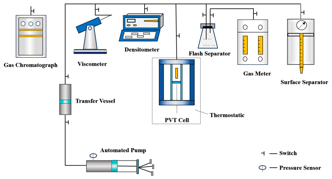
To perform CCE and CVD experiments under both equilibrium and non-equilibrium conditions, a high-temperature and high-pressure PVT experimental setup was designed and constructed. The PVT analysis apparatus and workflow for reservoir fluids are shown in Figure 1. The apparatus consists of an automated pump, a temperature control system, a densitometer, a chromatograph, a viscometer, a flash separator, a gas meter, and a PVT cell. The temperature control system maintains a stable experimental temperature of 138.7 °C (±0.1 °C). The densitometer and viscometer facilitate real-time monitoring of fluid density (±0.5 kg/m³) and viscosity (±0.01 mPa·s). The chromatograph determines the mole fraction of each component with an accuracy of ±0.2%. In addition, the flash separator and gas meter are used to achieve precise phase separation and accurate measurement of the produced gas volume.

2.2.2. Experimental Methods and Procedures

Prior to each experiment, the PVT cell was thoroughly evacuated to eliminate any residual gases and subsequently heated to the reservoir temperature of 138.7 °C. Under isothermal conditions, the recombined condensate gas sample was transferred into the PVT cell and pressurized to the reservoir pressure of 48 MPa. The initial sample volume (V) was recorded as a reference for all subsequent equilibrium and non-equilibrium measurements.

(1)

Equilibrium Phase Behavior Experiments

Equilibrium phase behavior experiments were conducted using the stepwise pressure reduction method in accordance with the aforementioned national standard. At each pressure step, the fluid was mechanically stirred to promote complete mixing, followed by a static period to allow the system to reach thermodynamic equilibrium. During this process, key phase behavior data were obtained. These data included the dew point pressure and volume determined from the CCE test as well as the retrograde condensate saturation measured and recovery factor calculated from the CVD test. The latter was obtained by measuring the volumes of gas and liquid phases at each pressure step.

(2)

Non-Equilibrium Phase Behavior Experiments

Non-equilibrium phase behavior experiments were conducted under the same temperature and pressure conditions as the equilibrium tests but without stirring. This is to avoid artificially enhancing mass transfer and to ensure that the observed effects reflect the intrinsic influence of pressure depletion rate on the phase transition process, in order to capture the effects of rapid pressure depletion on the phase transition process. Five distinct pressure depletion rates were investigated: 3, 5, 7, 10, and 15 MPa/h. In the non-equilibrium CCE experiments, the pressure was continuously reduced from 48 MPa to the abandonment pressure of 10 MPa at the specified depletion rates, while pressure and volume data were rapidly recorded in real time. In the non-equilibrium CVD experiments, depletion began at the dew point pressure, and the PVT volume was maintained constant as pressure was further decreased. At each pressure step, the gas-phase volume and composition were measured rapidly. Based on these data, the condensate recovery factor and retrograde condensate saturation were subsequently calculated.

All experimental runs were across the five depletion rates to comprehensively evaluate the influence of pressure depletion rate on non-equilibrium phase transition behavior and to establish a quantitative basis for model validation.

It should be noted that, although mechanical stirring was intentionally avoided to minimize artificial enhancement of mass transfer, molecular diffusion and weak natural convection may still occur within the PVT cell. Therefore, the present experimental design does not completely isolate depletion-rate effects from all transport mechanisms. However, due to the relatively small characteristic length scale of the PVT cell and the strictly controlled isothermal conditions, these secondary transport effects are significantly constrained. Under such conditions, the pressure depletion rate remains the dominant factor governing phase transition kinetics.

2.3. Uncertainty Analysis and Experimental Limitations

The equilibrium experiments were used as thermodynamic reference measurements, whereas the non-equilibrium experiments were designed to capture rate-dependent phase-transition behavior under continuous pressure depletion. Therefore, the comparison between the two experimental modes focuses on systematic depletion rate-dependent trends rather than small point-wise deviations.

The experimental apparatus was equipped with high-precision sensors to minimize systematic errors. The pressure transducers maintain an accuracy of ±0.01 MPa, while the temperature of the PVT cell was controlled within a stability range of ±0.1 °C using a high-precision thermostatic bath. For the volumetric measurements, the liquid-phase volume was recorded with an optical cathetometer providing a resolution of ±0.005 cm³.

To ensure experimental repeatability, triplicate non-equilibrium CCE and CVD experiments were conducted at each pressure depletion rate of 3, 5, 7, 10, and 15 MPa/h under identical operating conditions. The measured relative volume, retrograde condensate saturation, and condensate recovery factor were averaged and used for subsequent model calibration and validation. The saturation-pressure measurements showed good consistency within the instrumental uncertainty, while the relative deviations of the calculated phase-behavior parameters among the three repeated runs were generally below 5%. This indicates that the observed depletion rate-dependent non-equilibrium behavior was reproducible rather than being caused by random experimental fluctuations.

3. Model Development

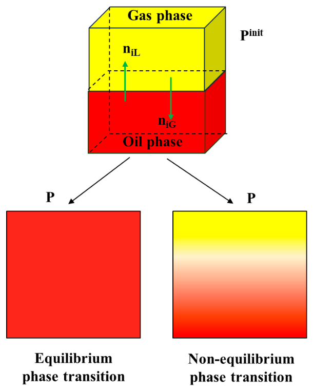
The model conceptually illustrates the distinction between the theoretical equilibrium assumption and the actual phase transition process (Figure 2). At the initial pressure (P^init), a stable gas–oil interface forms as the system attains thermodynamic equilibrium. Classical equilibrium theory assumes that any change in pressure leads to an instantaneous adjustment to a new homogeneous equilibrium state. However, in practice phase transitions are inherently time-dependent, and the system approaches the new equilibrium state gradually as interphase mass transfer progresses. During reservoir production, the characteristic relaxation time is often insufficient for complete equilibration, resulting in persistent non-equilibrium behavior that directly influences fluid phase properties and reservoir performance.

3.1. Physical Basis and Model Assumptions

In condensate-gas reservoirs, pressure depletion induces a non-equilibrium phase behavior characterized by a lag between the evolving system state and the corresponding thermodynamic equilibrium. This deviation arises from the finite-rate nature of interphase mass transfer and compositional redistribution, which prevents instantaneous equilibration when pressure drops below the dew point. As a result, macroscopic properties such as condensate saturation and relative volume exhibit rate-dependent departures from equilibrium under dynamic depletion conditions.

From a thermodynamic perspective, phase evolution is driven by fugacity or chemical potential differences between phases, which act as the fundamental driving force for interphase mass exchange. At the microscopic scale, these processes are governed by diffusion and interfacial mass transfer. However, explicit resolution of multicomponent transport and interface dynamics is computationally intractable for reservoir-scale applications. Therefore, their collective effect is represented in this work through a physics-informed reduced-order formulation.

In this framework, the effective relaxation rate α is introduced as an apparent lumped parameter to describe the macroscopic approach of the system toward equilibrium, rather than as a directly measured molecular diffusion coefficient. A simple transport scaling can be expressed as $({\mathrm{t}}_{\mathrm{D}}~L_C^2/D_{eff})$, where $L_C$ is the characteristic transport length and $D_{eff}$ is the effective multicomponent diffusion coefficient. Since local diffusion coefficients, interfacial area evolution, and condensate-domain length scales were not directly measured in this work, $\alpha$ is interpreted as a reduced-order macroscopic parameter that integrates the combined effects of molecular diffusion, interfacial mass transfer, and compositional redistribution. By coupling this apparent relaxation timescale with the external pressure depletion rate, the model captures the competition between thermodynamic driving forces and kinetic resistance.

The formulation of the model is based on the following assumptions:

• The process occurs under isothermal conditions.
• During rapid pressure depletion, the system remains in a dynamic non-equilibrium state.
• The return to equilibrium is controlled by finite-rate interphase mass transfer and compositional redistribution, whose net effect can be represented by an effective relaxation rate, $\alpha$.
• The relaxation rate is assumed to depend on the pressure depletion rate, reflecting the competition between external forcing and internal relaxation timescales.
• The formulation integrates species-wise diffusion, interfacial area evolution, and detailed local transport processes into the effective relaxation parameter.

Under this formulation, deviations from equilibrium are interpreted as the macroscopic manifestation of incomplete relaxation. A higher relaxation rate corresponds to faster equilibration, whereas rapid depletion reduces the effective time available for mass transfer, leading to enhanced non-equilibrium effects. This provides the physical basis for the dynamic phase transition model developed in the following section.

3.2. Non-Equilibrium Phase Transition Model

Equilibrium and non-equilibrium phase behavior experiments were conducted to measure key phase behavior parameters across a range of pressures ($P$). These parameters were categorized into two distinct sets. The equilibrium parameters, such as the equilibrium retrograde condensate saturation ($S^{eq}$), the relative volume ($V^{eq}$), and the recovery factor (${\eta }^{eq}$), were obtained under static conditions. In contrast, the corresponding non-equilibrium state parameters ($S^{neq}$, $V^{neq}$, ${\eta }^{neq}$) were derived under dynamic pressure-depletion conditions. Rapid pressure depletion during non-equilibrium experiments introduces thermodynamic imbalances, resulting in discrepancies between equilibrium characteristic parameters (${\phi }^{eq}(P)$) and non-equilibrium characteristic parameters (${\phi }^{neq}(P)$). These deviations quantify non-equilibrium effects during pressure depletion. Accordingly, the deviation of non-equilibrium characteristic parameters relative to their equilibrium counterparts can be expressed as follows:

$$∆\phi (P)={\phi }^{eq}(P)-{\phi }^{neq}(P)$$

(1)

This deviation quantifies the degree to which the system lags behind the equilibrium phase state during pressure depletion. Physically, such deviation originates from the fact that pressure reduction below the dew point creates a thermodynamic imbalance between phases, generating a driving force for interphase mass transfer and compositional redistribution.

At the microscopic scale, the interphase molar flux of component ii is driven by fugacity or chemical potential differences:

$$J_i=k_{i}a(f_i^g-f_i^l)$$

(2)

where $J_i$ is the interphase transfer rate of component $i$, $k_i$ is the effective mass-transfer coefficient, $\alpha$ is the effective interfacial area, and $f_i^g$ and $f_i^l$ represent the fugacity of component $i$ in the gas and liquid phases, respectively.

Given the significant computational complexity associated with resolving all individual $J_i$ in a reservoir-scale model, the combined influence of all components on the macroscopic phase-state deviation $∆\phi$ is effectively captured by introducing a lumped thermodynamic driving force:

$${\Phi }_{drive}(P)={\displaystyle \sum _i{\omega }_i}\cdot (f_i^g(P)-f_i^l(P))$$

(3)

where ${\omega }_i$ are weighting coefficients that account for the contribution of each component to the observed phase property (e.g., saturation or relative volume). The rate of change of $∆\phi$ is then linearly related to this lumped driving force (Buleyko [41]):

$${\displaystyle \frac{d(∆\phi )}{dt}}=\beta \cdot {\Phi }_{drive}(P)$$

(4)

Within a small pressure interval and under non-equilibrium conditions, the lumped driving force can be linearly approximated as proportional to the current deviation from equilibrium (consistent with Onsager’s linear phenomenological relations in irreversible thermodynamics):

$${\Phi }_{drive}(P)\approx \gamma \cdot ∆\phi (t)$$

(5)

Substituting Equation (5) into Equation (4) yields a first-order relaxation kinetic equation:

$${\displaystyle \frac{d(∆\phi )}{dt}}=-\alpha \cdot ∆\phi (t)$$

(6)

where $\alpha =-\beta \gamma >0$ is the effective relaxation rate. The negative sign indicates that the system evolves toward equilibrium ($∆\phi \to 0$). This expression indicates that the instantaneous rate of approach toward equilibrium is proportional to the current magnitude of deviation. The above formulation can be interpreted as the reduced-order consequence of interphase mass transfer: the farther the system is from equilibrium, the stronger the restoring tendency; the slower the effective transport process, the smaller the relaxation rate and the longer the persistence of non-equilibrium behavior.

Equation (6) is a separable ordinary differential equation. Integrating from the reference pressure $P_{ref}$ (where deviation first becomes noticeable) to an arbitrary pressure $P$:

$${\displaystyle {\int }_{∆\phi (P_{ref})}^{∆\phi (P)}\frac{d(∆\phi )}{∆\phi }}=-\alpha {\displaystyle {\int }_{t(P_{ref})}^{t(P)}dt}$$

(7)

yields:

$$∆\phi \left(P\right)=∆\phi \left(P_{ref}\right)e^{-\alpha \left(t(P)-t(P_{ref})\right)}$$

(8)

At $P_{ref}$ the initial deviation is defined as:

$$∆\phi (P_{ref})={\phi }^{eq}(P_{ref})-{\phi }^{neq}(P_{ref})$$

(9)

Substituting Equation (9) into Equation (8) and combining it with Equation (1) results in the simplified dynamic model for non-equilibrium phase behavior:

$${\phi }^{neq}(P)={\phi }^{eq}(P)+[{\phi }^{neq}(P_{ref})-{\phi }^{eq}(P_{ref})]\cdot e^{-\alpha \left(t(P)-t(P_{ref})\right)}$$

(10)

In general, the relaxation timescale is governed by diffusion and interphase mass transfer processes and can be expressed in terms of an effective diffusion coefficient and mass-transfer coefficient as:

$$\tau \sim {\displaystyle \frac{L^2}{D_{eff}}}+{\displaystyle \frac{1}{k_{m}a}}$$

(11)

And the characteristic relaxation rate is defined as the inverse of the effective relaxation timescale:

$$\alpha ={\displaystyle \frac{1}{\tau }}$$

(12)

The dependence of the relaxation rate $\alpha$ on the depletion rate is introduced as a closure relation to account for unresolved multicomponent transport processes, rather than being strictly derived from first-principles transport equations. Physically, this formulation reflects the competition between the externally imposed depletion timescale and the intrinsic mass-transfer relaxation timescale.

This timescale analysis provides a physical constraint on the functional form of the relaxation rate. Specifically, the competition between the depletion timescale and the relaxation timescale implies that the effective relaxation process cannot remain constant but must vary with the external forcing intensity. Therefore, the dependence of $\alpha$ on ($dp/dt$) is not arbitrary, but represents a reduced-order manifestation of this timescale imbalance.

Accordingly, the relaxation rate is expressed as:

$$\alpha ={\alpha }_0\cdot \left[1+k_p\cdot {({\displaystyle \frac{∆p}{∆t}})}^n\right]$$

(13)

In Equation (13), the base relaxation rate ${\alpha }_0(h^{-1})$ reflects the intrinsic relaxation capacity of the fluid system to reach equilibrium under slow pressure depletion or near-equilibrium conditions. Its value is primarily determined by fluid composition, pressure, temperature, and physical properties. The coefficient $k_p{(MPa/h)}^{-n}$ quantifies the sensitivity of the relaxation rate to external pressure dynamics, characterizing the degree to which variations in the pressure depletion rate influence the relaxation process. A larger k_p corresponds to a stronger coupling between external pressure changes and internal relaxation kinetics. The nonlinear amplification term ${(∆p/∆t)}^n$ further captures the dependence of relaxation on depletion rate, where the exponent $n$ governs the degree of nonlinearity. As $n$ increases, relaxation effects become more pronounced at higher pressure depletion rates, highlighting the nonlinear nature of non-equilibrium phase transition in reservoir fluids.

These three parameters are not intended to be universal constants. Instead, they represent fluid-dependent kinetic descriptors that summarize the combined effects of composition, phase-envelope characteristics, transport properties, and interphase mass-transfer resistance on the relaxation process. Therefore, when the model is applied to another condensate-gas system or to other rate-sensitive hydrocarbon fluids, the same model structure may be retained, but ${\alpha }_0$, $k_p$, and $n$ should be re-estimated from the corresponding experimental dataset.

By substituting Equation (13) into Equation (10), the final model is obtained:

$${\phi }^{neq}(P)={\phi }^{eq}(P)+[{\phi }^{neq}(P_{ref})-{\phi }^{eq}(P_{ref})]\cdot e^{-{\alpha }_0\times \left[1+k_p\cdot {({\displaystyle \frac{∆p}{∆t}})}^n\right]\times \left[t(P)-t(P_{ref})\right]}$$

(14)

To explicitly determine this model, three key parameters must be identified: the base relaxation rate (${\alpha }_0$), the pressure depletion sensitivity coefficient ($k_p$), and the nonlinearity exponent ($n$). These parameters are estimated by fitting the model to non-equilibrium experimental data through an optimization procedure. The least squares method is employed to minimize the deviation between the experimentally measured non-equilibrium deviation ${\phi }_k^{neq}$ and the corresponding model-predicted value ${\phi }_k^{neq,\mathrm{mod}el}$.

$$minimize{\displaystyle \sum _k{[{\phi }_k^{neq}-{\phi }_k^{neq,model}]}^2}$$

(15)

where ${\phi }_k^{neq}$ represents the values of the experimentally measured non-equilibrium characteristic parameters at the $k-th$ pressure step ($k=1,2,\dots ,m$). This fitting procedure optimizes the parameter set (${\alpha }_0$, $k_p$, and $n$) to ensure that the model accurately reproduces the relaxation kinetics observed in experiments. Consequently, this enables a quantitative prediction of dynamic phase behavior under varying pressure depletion conditions.

Based on the results obtained from Equation (15), the optimized parameters ${\alpha }_0$, $k_p$, and $n$ are substituted into Equation (14). This substitution yields an explicit expression for the characteristics of non-equilibrium phase transitions, which are expressed as functions of pressure depletion rate and fitted kinetic parameters.

3.3. Model Parameter Estimation and Calibration

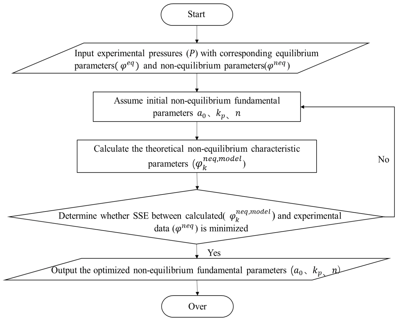
Based on the established non-equilibrium dynamic phase transition model, this study determined the characteristic parameters by fitting experimental data under different pressure conditions using the least squares method. The optimized values of ${\alpha }_0$, $k_p$, and $n$ were obtained through this process. Initially, equilibrium and non-equilibrium characteristic parameters (${\phi }^{eq}$ and ${\phi }^{neq}$) at various pressures ($P$) were derived from the experimental data. Initial estimates for the base relaxation rate (${\alpha }_0$), the pressure depletion sensitivity coefficient ($k_p$) and the exponent ($n$) were assigned. Using these initial values, the theoretical non-equilibrium characteristic parameters (${\phi }_k^{neq,model}$) were calculated at different pressure depletion rates according to Equation (8). The Sum of Squared Errors (SSE) between the model predictions and the experimental values was then evaluated. The parameters ${\alpha }_0$, $k_p$, and $n$ were iteratively adjusted to minimize the SSE, with calculations repeated until convergence was achieved. Once convergence was achieved, the parameter set (${\alpha }_0$, $k_p$, $n$) was substituted into the dynamic phase transition model to calculate the relaxation rate ($\alpha$) under varying pressure depletion rates. This facilitated a quantitative analysis of the characteristic relaxation time and non-equilibrium characteristic parameters at various pressure depletion rates.

The complete computational workflow is illustrated in Figure 3, which outlines the iterative process and ensures the model’s reliability with experimental observations.

4. Results and Discussion

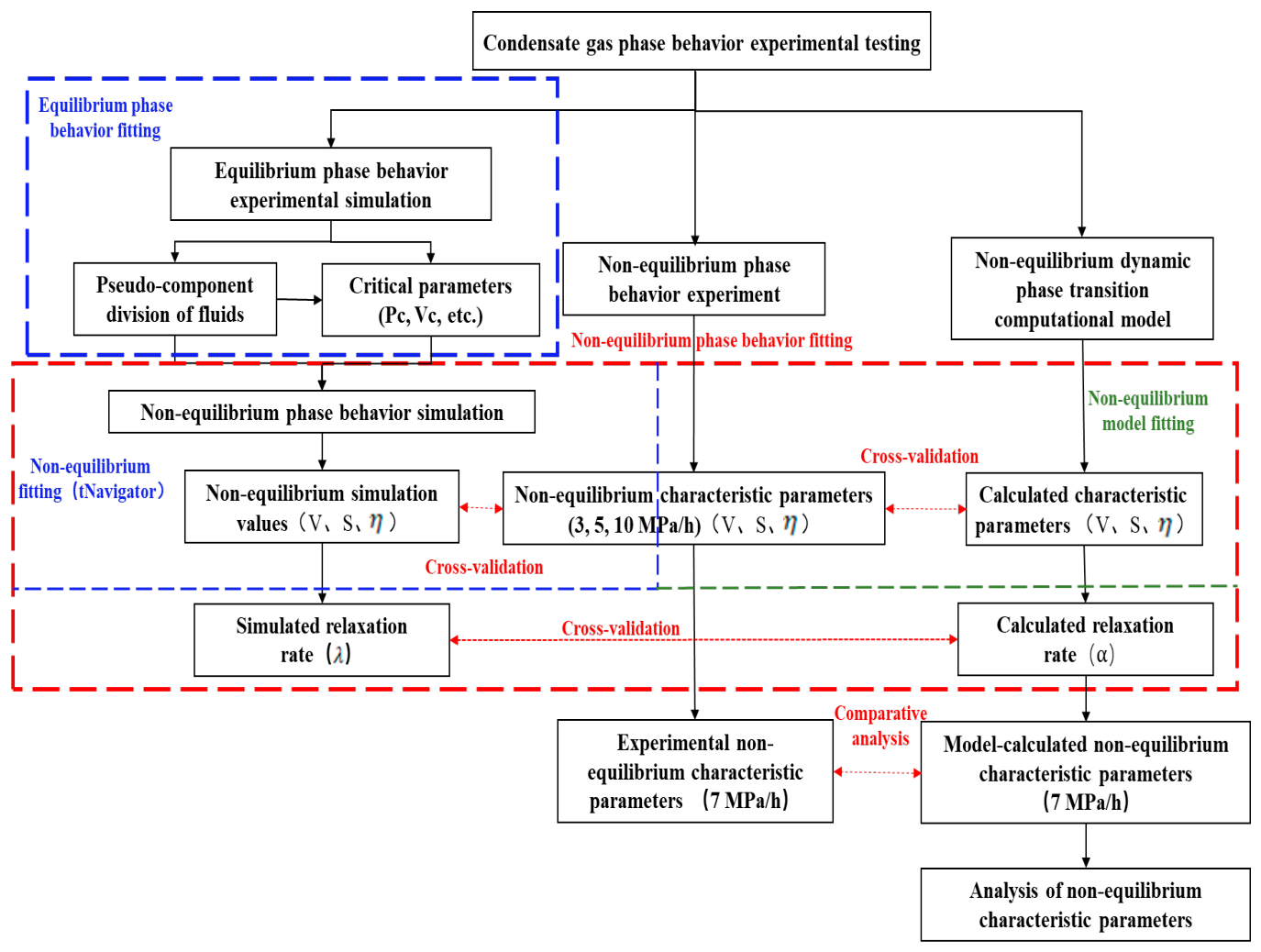
To verify the reliability of the proposed non-equilibrium dynamic phase transition model, a hierarchical validation framework was implemented. The experimental data were partitioned into a calibration set (3, 5, and 10 MPa/h) and an internal hold-out validation dataset (7 and 15 MPa/h). The overall workflow is illustrated in Figure 4.

In the first stage, equilibrium phase behavior data were fitted using the tNavigator (version 21.1, ROCKFLOW Dynamics) simulator to establish pseudo-components and determine critical parameters (e.g., critical temperature (T_c), critical pressure (P_c), etc.). These parameters provided the thermodynamic foundation for subsequent non-equilibrium modeling.

In the second stage, a dual-method consistency check was performed. The non-equilibrium experimental data at depletion rates of 3, 5, and 10 MPa/h were used to calibrate the relaxation parameters within the proposed model. Simultaneously, tNavigator was utilized as a benchmark for comparison. The close agreement between the proposed model and the simulator-based results confirms the internal consistency and physical accuracy of the model in reproducing the non-equilibrium kinetics observed in the experiments.

To further evaluate the predictive capability of the proposed model, hold-out predictions were performed using depletion rates of 7 MPa/h and 15 MPa/h, which were strictly excluded from the parameter-calibration process. The agreement between the hold-out predictions and experimental measurements indicates that the model can reproduce the depletion-rate-dependent non-equilibrium response within the studied condensate-gas system. This result should not be interpreted as evidence of cross-fluid or cross-reservoir extrapolative capability. Rather, it demonstrates that the proposed framework retains predictive capability for depletion conditions that were not included in the calibration dataset, thereby reducing the likelihood that the observed agreement arises solely from regression fitting. Although the present study is limited to a single condensate-gas fluid system, the hold-out validation supports the applicability of the model for describing the dynamic phase-transition response within the investigated fluid system.

4.1. Numerical Simulation

4.1.1. Equilibrium Phase Behavior Fitting

Based on the experimental data of equilibrium phase behavior, phase behavior simulations were carried out to establish a representative fluid model. The reservoir fluid was categorized into six pseudo-components, in which the heavy fraction (C₇₊) was treated as a lumped component and calibrated during EOS tuning. Although simplified, this treatment is commonly adopted in gas-condensate EOS modeling and provides a practical balance between compositional complexity and predictive capability. The C₇₊ fraction was characterized using standard critical property correlations and further tuned during regression to match experimental phase behavior. The equilibrium PVT simulations were performed using the Peng–Robinson equation of state implemented in tNavigator.

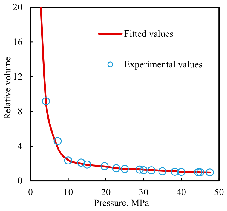
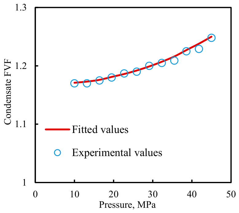
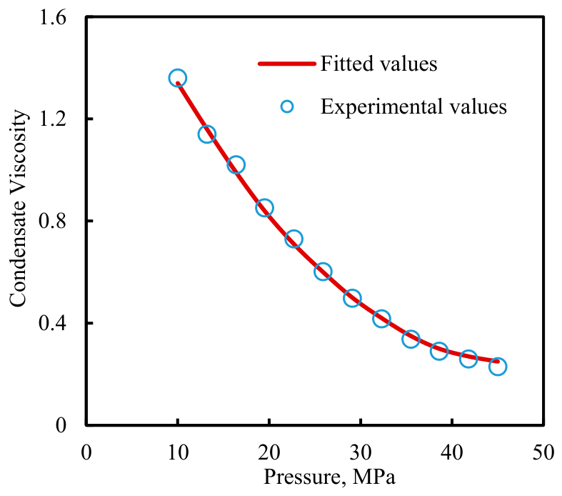
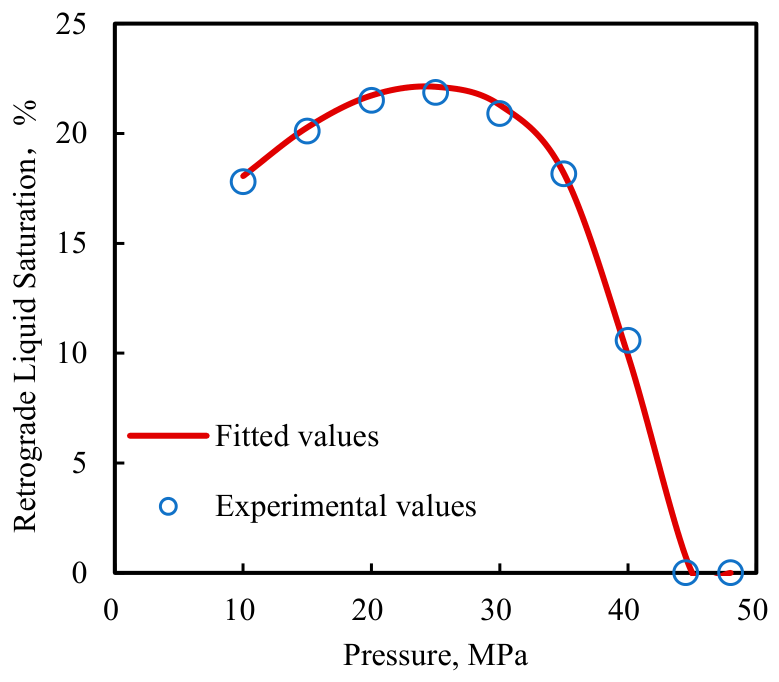
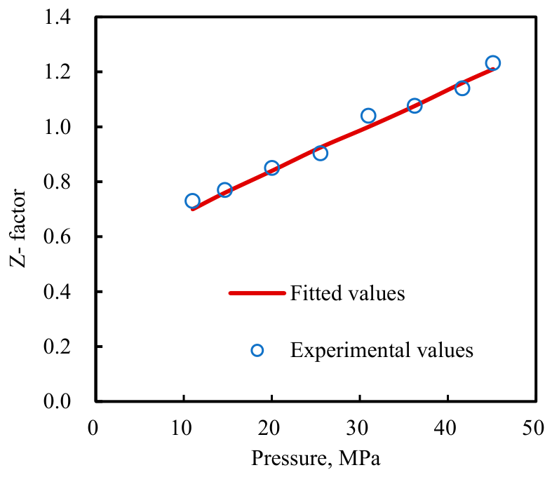
The thermodynamic parameters of the pseudo-components—including critical temperature (Tc), critical pressure (Pc), acentric factor ($\omega$) for heavy fractions, and binary interaction coefficients ($k_{ij}$)—were optimized through regression against experimental measurements. The binary interaction coefficients ($k_{ij}$) were adjusted iteratively to minimize deviations in saturation pressure, phase boundary, and compositional distribution between experimental and simulated results. The tuning procedure was constrained by simultaneously matching dew point pressure, phase envelope, and compositional distribution, ensuring physical consistency of the optimized parameters. This pseudo-component scheme effectively reproduces both the compositional distribution and the phase behavior characteristics of the condensate gas system, as well as key PVT properties such as viscosity and formation volume factor (FVF). The regression outcomes are summarized in

Table 2. Pseudo-components of condensate-gas fluid.

Component	Mole Fraction, mol%	Critical Temperature, K	Critical Pressure, MPa	Acentric Factor	Molecular Weight, g/mol	Molar Volume, ×10−3 m3/mol	Boiling Point, K
CO2	5.77	304.19	7.38	0.23	44.01	0.09	194.69
N2	1.54	126.20	3.46	0.04	28.01	0.09	77.34
C1	77.22	154.06	5.40	0.01	19.05	0.08	111.67
C2–C3	5.08	310.07	5.55	0.10	40.41	0.14	196.64
C4+	3.10	524.07	4.11	0.26	75.05	0.25	304.50
C7+	6.68	647.22	1.89	0.42	85.04	0.31	386.02

and Figure 5, Figure 6, Figure 7, Figure 8 and Figure 9, which demonstrate good agreement between experimental and simulated results.

The EOS tuning provided satisfactory agreement with the measured dew point pressure, flash properties, and major phase-behavior trends for the condensate-gas system investigated in this study (

Table 3. Comparison of key parameter fitting results for condensate gas.

Property	Experimental Value	Simulated Value	Relative Error, %
Gas–Oil Ratio, GOR	1268	1269.8	0.13
Flash Oil Density, g/cm3	0.702	0.804	1.45
Dew Point Pressure, MPa	45	45	0

). Nevertheless, the tuned EOS model should not be regarded as uncertainty-free. Because the full covariance matrix of the EOS regression parameters was not available from the commercial simulator, a rigorous EOS-parameter uncertainty propagation was not performed. Instead, the uncertainty analysis in this work was treated in a sensitivity-based manner by considering the experimental uncertainty and its influence on the fitted relaxation parameters. Therefore, the EOS model is used as a thermodynamic reference for constructing equilibrium phase behavior, while the reported uncertainty intervals of the relaxation parameters should be interpreted as estimated uncertainty ranges rather than strict statistical confidence intervals.

4.1.2. Model Calibration and Benchmark Validation

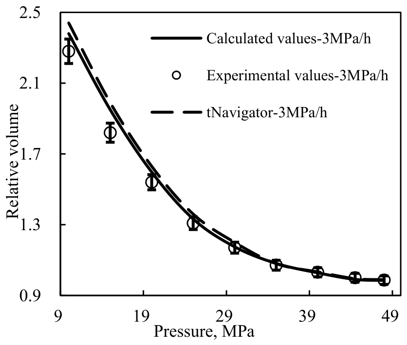
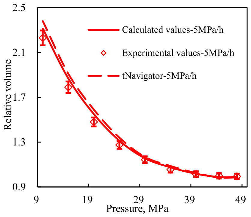
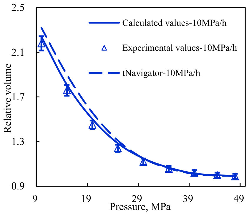
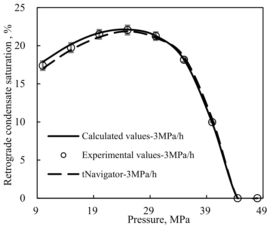
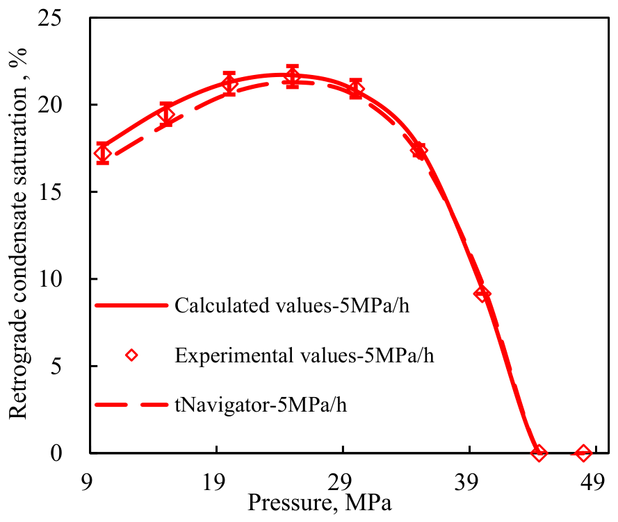
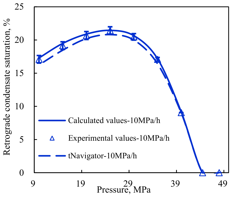
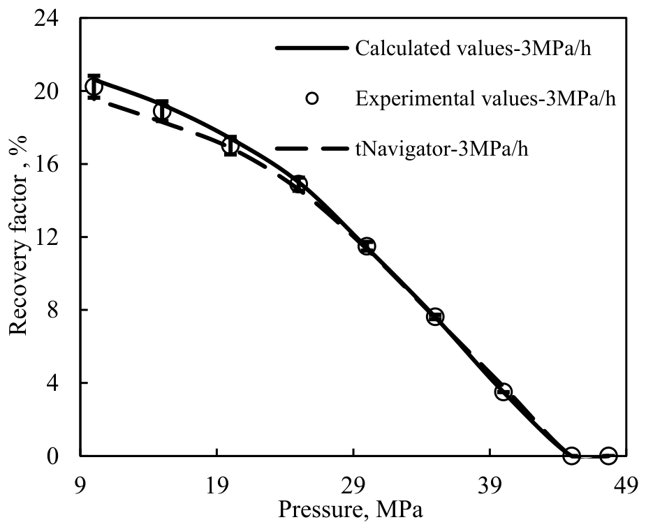
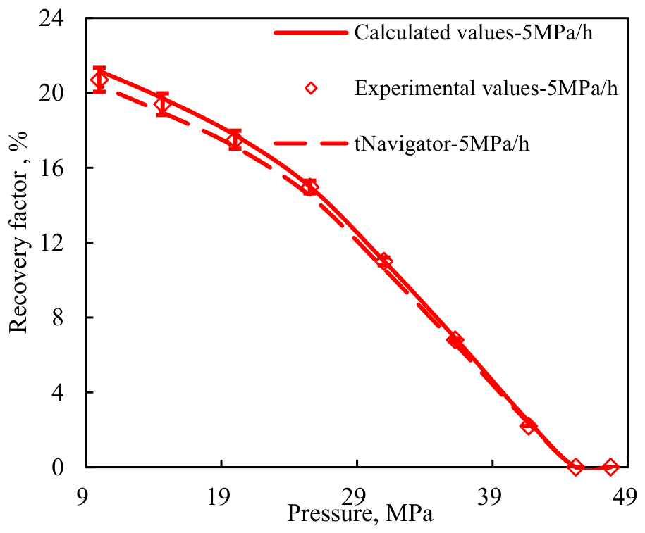
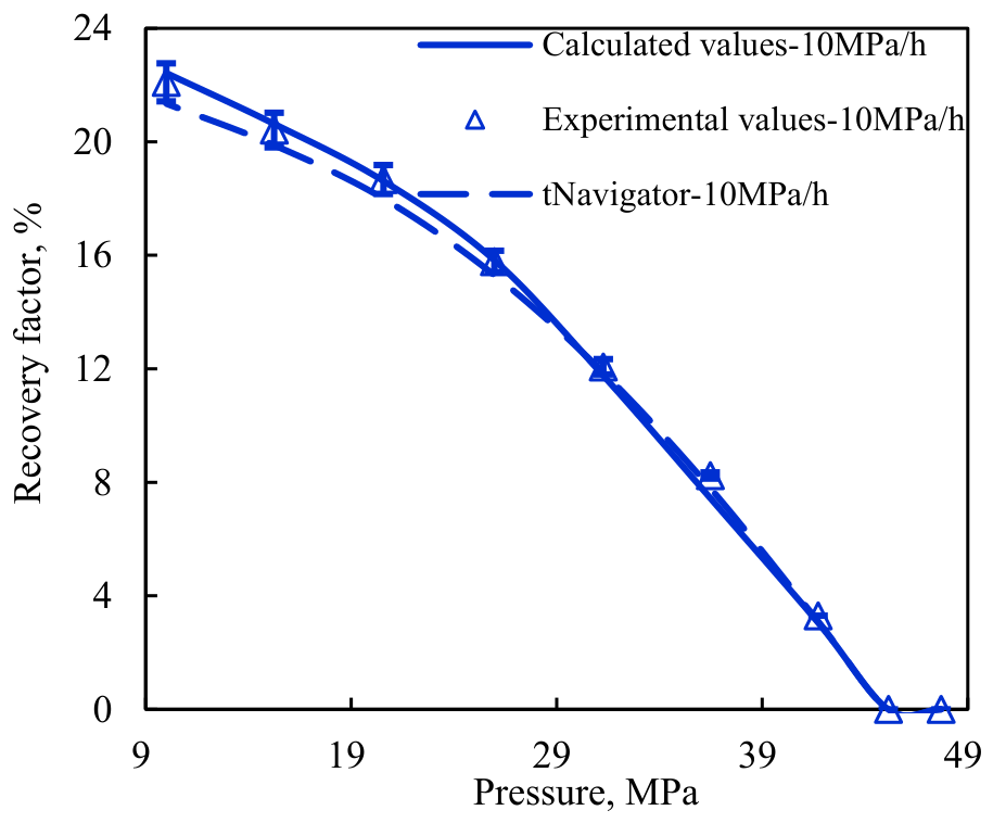
Following the validation of equilibrium phase behavior, the analysis was extended to non-equilibrium conditions, where rapid pressure depletion induces phase lag and deviations from equilibrium predictions. The experimental data from NCCE and NCVD at depletion rates of 3, 5, and 10 MPa/h were used for model calibration. The same datasets were also simulated using the tNavigator compositional simulator under identical conditions, enabling a direct benchmark comparison between the proposed model and a widely used numerical simulator.

To ensure reproducibility of the benchmark comparison, the tNavigator simulations were performed using the tuned compositional fluid model described in Section 4.1.1. The equilibrium flash calculation was based on the Peng–Robinson equation of state with six pseudo-components, and the pseudo-component properties and binary interaction coefficients obtained from the equilibrium PVT regression were kept unchanged during the non-equilibrium calculations. The laboratory NCCE and NCVD processes were reproduced by imposing the same isothermal pressure-depletion schedules as those used in the experiments, with depletion rates of 3, 5, and 10 MPa/h for the benchmark calibration cases. In the tNavigator benchmark, phase-transition delay was represented using a relaxation-controlled non-equilibrium treatment, in which the approach of the fluid state toward the corresponding equilibrium flash state was governed by an effective relaxation rate. The tNavigator-derived relaxation rates were then compared with those predicted by the proposed analytical model.

As shown in

Table 4. Average relative errors at different depletion rates, %.

Pressure Depletion Rate, MPa/h	Relative Volume		Retrograde Condensate Saturation		Condensate Recovery Factor
	Model	tNavigator	Model	tNavigator	Model	tNavigator
3	1.99	1.25	1.06	2.54	1.81	2.82
5	2.03	1.36	1.39	3.01	2.05	3.13
10	2.08	2.17	1.68	3.58	2.85	3.42
Average	2.03	1.59	1.38	3.04	2.23	3.12

Note: The average relative error (ARE) is a statistical metric used to evaluate the overall deviation between model-calculated values and measured data. It reflects the average deviation ratio over a dataset and is calculated as: $Average Relative Error (ARE)={\displaystyle \frac{1}{n}}{\displaystyle {\sum }_{i=1}^n\left|\frac{y_i-{\widehat{y}}_i}{y_i}\right|}\times 100\%$.

and Figure 10, Figure 11, Figure 12, Figure 13, Figure 14, Figure 15, Figure 16, Figure 17 and Figure 18, both methods effectively reproduced the key parameters of non-equilibrium phase behavior. The proposed model consistently achieved average relative errors ranging from 1.38% to 2.23%, whereas the tNavigator results ranged from 1.59% to 3.12%. This comparison indicates that both approaches achieve good prediction accuracy under the same conditions.

The optimized parameters obtained from the proposed model are summarized in

Table 5. Optimized parameters and estimated uncertainty intervals of the dynamic phase transition model.

Basic Parameter	Optimized Value	Estimated Uncertainty	Estimated Uncertainty Interval
$\mathrm{Baseline} \mathrm{Relaxation} \mathrm{Rate} {\alpha }_0$, 1/h	0.5	±0.035	0.465–0.535
$\mathrm{Rate} \mathrm{Sensitivity} \mathrm{Coefficient} k_p$, MPa/h−n	−0.474	±0.028	−0.502–0.446
Index $n$	0.152	±0.012	0.140–0.164

. The estimated uncertainty intervals of the fitted parameters were evaluated based on the experimental uncertainty range obtained from the repeatability analysis and parameter-sensitivity assessment. These parameters quantitatively characterize the nonlinear coupling between depletion dynamics and relaxation behavior, allowing the model to effectively capture the continuous transition from near-equilibrium to strongly non-equilibrium states. As listed in

Table 6. Relaxation parameters at different pressure depletion rates.

Pressure Depletion Rate, MPa/h	Relaxation Rate, 1/h		Non-Equilibrium Relaxation Time, h	Estimated τ Interval, h	Relative Error of Relaxation Rate, %
	tNavigator	Model
3	0.2160	0.2062	4.85	4.62–5.10	4.54
5	0.1736	0.1774	5.64	5.37–5.93	1.28
10	0.1534	0.1484	6.74	6.42–7.09	3.36

, the calculated relaxation rates and times exhibit a clear inverse relationship with the depletion rate. Specifically, when the depletion rate increased from 3 to 10 MPa/h, the relaxation rate decreased from 0.2062 to 0.1484 h⁻¹, while the characteristic relaxation time extended from 4.85 h to 6.74 h. This trend indicates that rapid pressure depletion suppresses interphase mass transfer and delays component redistribution, thereby prolonging the time required to achieve equilibrium.

It should also be emphasized that the optimized parameters ${\alpha }_0$, $k_p$ and $n$ obtained in this study should be regarded as fluid-specific kinetic descriptors rather than universal constants. The baseline relaxation rate ${\alpha }_0$ reflects the intrinsic capacity of the investigated fluid system to approach equilibrium under slow-depletion or near-equilibrium conditions, and is therefore related to fluid composition, phase-envelope characteristics, viscosity, diffusion behavior, and interphase mass-transfer resistance. The parameters $k_p$ and $n$ describe the sensitivity and nonlinear response of the relaxation rate to the imposed pressure depletion rate; consequently, their values may vary among different condensate-gas systems with different heavy-end contents, dew point pressures, liquid-dropout tendencies, and compositional redistribution kinetics. Nevertheless, the governing model framework is transferable in principle, because it is formulated based on the general competition between the external pressure-depletion timescale and the intrinsic phase-relaxation timescale. For another condensate-gas fluid or other rate-sensitive hydrocarbon systems such as volatile oils, the same model structure can be retained, but ${\alpha }_0$, $k_p$ and $n$ should be recalibrated using the corresponding non-equilibrium phase-behavior experimental data before predictive application.

$$\alpha =0.5\times \left[1-0.474\times {({\displaystyle \frac{∆p}{∆t}})}^{0.152}\right]$$

(16)

From a qualitative perspective, these results reveal the intrinsic kinetics of phase transitions in condensate-gas systems. When reservoir pressure declines rapidly, the rate of external pressure reduction surpasses the ability of components to redistribute between gas and liquid phases, leading to enlarged concentration gradients across the phase boundary. This phenomenon intensifies interphase mass-transfer resistance, prolongs the relaxation process, and magnifies the degree of deviation from equilibrium. In contrast, under slower depletion rates, molecular diffusion and phase redistribution have sufficient time to proceed, allowing the system to remain closer to thermodynamic equilibrium, which results in higher relaxation rates and shorter characteristic relaxation times.

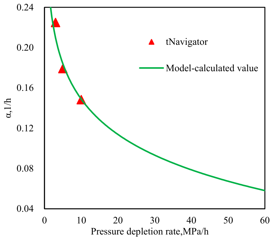
The tNavigator-derived relaxation rates listed in Table 6 were obtained from the relaxation-controlled non-equilibrium matching under the same depletion schedules and were used only as benchmark values for comparison with the proposed analytical model.

This trend is further illustrated in Figure 19, where the relaxation rate ($\alpha$) exhibits an exponential decline with increasing depletion rate. Two distinct kinetic regimes emerge. At low depletion rates (<5 MPa/h), $\alpha$ remains relatively high (>0.177 h⁻¹), suggesting that non-equilibrium effects are weak and phase transitions occur nearly in step with pressure changes. Conversely, at higher depletion rates (>10 MPa/h), $\alpha$ falls below 0.1484 h⁻¹, indicating strong constraints on phase transition dynamics, a noticeable lag in condensate precipitation, and significant deviations in overall fluid composition. This exponential dependence highlights the rate-controlled nature of non-equilibrium phase transitions, as faster pressure depletion increasingly limits the system’s ability to achieve compositional and phase equilibrium.

The calculated relaxation times are consistent with the order-of-magnitude transport scaling discussed in Section 3.1, indicating that the fitted α values are physically reasonable as apparent macroscopic relaxation parameters for the studied condensate-gas system.

These insights indicate that production strategies involving rapid pressure depletion can exacerbate non-equilibrium effects and significantly alter condensate dropout and recovery behavior. Conversely, moderated depletion strategies help preserve system equilibrium, mitigate adverse compositional shifts, and enhance the condensate recovery factor. Therefore, the proposed model provides strong quantitative agreement with measurements and, more importantly, offers mechanistic understanding and practical guidance for reservoir management.

4.2. Internal Hold-Out Validation Within the Studied Condensate-Gas System

To assess the predictive capability of the proposed model within the investigated condensate-gas fluid system, an internal hold-out validation strategy was adopted. The experimental dataset was partitioned into two subsets: (1) a calibration dataset including depletion rates of 3, 5, and 10 MPa/h, which was used for parameter estimation; (2) a hold-out validation dataset including depletion rates of 7 and 15 MPa/h, which was excluded from the regression process and used only for post-calibration prediction.

It should be emphasized that this validation is internal to the studied condensate-gas system. Although the depletion rates of 7 and 15 MPa/h were not used for model calibration, all calibration and validation experiments were conducted using the same recombined condensate-gas fluid under the same reservoir temperature and fluid-composition conditions. Therefore, the validation primarily examines whether the model can interpolate and extrapolate the depletion-rate-dependent response within the same fluid system, rather than demonstrating full transferability across different reservoirs or hydrocarbon fluid types.

4.2.1. Model Calculations at 7 MPa/h and 15 MPa/h

The basic input parameters are summarized in

Table 7. Experimental reference data.

Characteristic Parameter	Equilibrium State	Non-Equilibrium State
		7 MPa/h	15 MPa/h
Relative Volume	1.028	1.019	1.012
Retrograde Condensate Saturation, %	9.884	9.161	9.149
Condensate Recovery Factor, %	3.522	4.014	4.203

, where equilibrium values are compared with non-equilibrium results at 7 and 15 MPa/h. The $P_{ref}$ is defined as the pressure at which characteristic parameters first exhibit notable deviations, typically occurring shortly after the pressure falls below the dew point. The time $t(P_{ref})$ required to reach $P_{ref}$ was determined to be 1.85 h from experimental data.

Using this data, the analytical expression for the non-equilibrium relative volume at 7 MPa/h is provided as follows:

$$V^{neq}(P)=V^{eq}(P)+(1.019-1.028)\times e^{-0.5\times (1-0.474\times 7^{0.152})\times \left(t(P)-1.85\right)}$$

(17)

This expression quantitatively relates equilibrium and non-equilibrium parameters, with corrections that depend on the depletion rate and time.

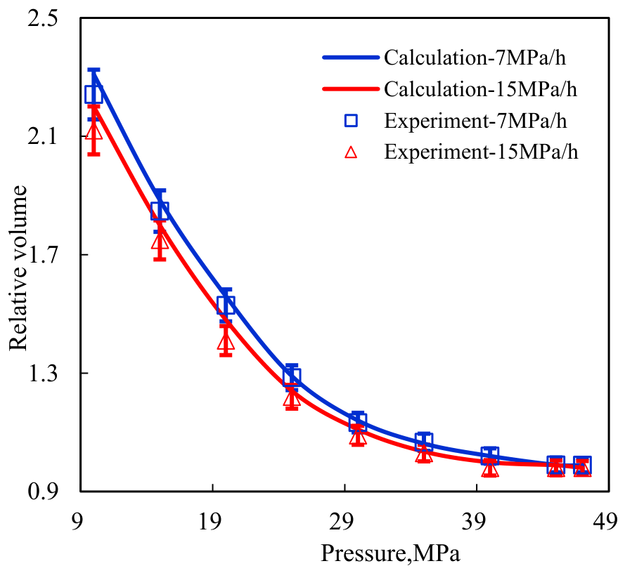
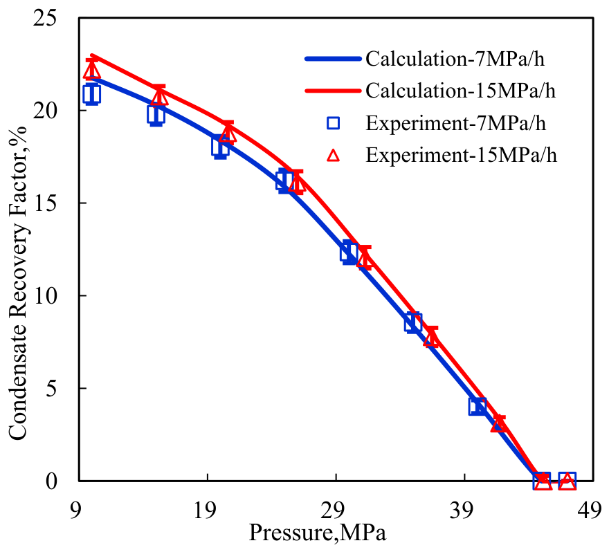
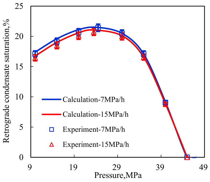
The calculated non-equilibrium parameters closely match the experimental data, with low average relative errors as shown in Figure 20, Figure 21 and Figure 22 and

Table 8. Average relative error of fitting at a pressure depletion rate, %.

Characteristic Parameter	7 MPa/h	15 MPa/h
Relative Volume	1.85	2.18
Retrograde Condensate Saturation	1.66	2.07
Condensate Recovery Factor	2.21	2.56

. As the pressure depletion rate increases from 7 MPa/h to 15 MPa/h, the relative volume error increases from 1.85% to 2.18%, the retrograde condensate saturation error from 1.66% to 2.07%, and the condensate recovery factor error from 2.21% to 2.56%. These comparisons confirm that the model effectively captures the influence of the depletion rate while maintaining a high level of predictive accuracy.

The good agreement between the predicted and measured results at 7 and 15 MPa/h indicates that the proposed model can capture the depletion rate-dependent non-equilibrium response of the studied condensate-gas fluid. However, the present validation does not cover compositional diversity, different reservoir temperatures, different condensate richness levels, or volatile-oil systems. Therefore, the current parameterized analytical model should be regarded as validated for the investigated condensate-gas fluid and for systems with comparable phase-behavior characteristics. Further validation using additional condensate-gas fluids, volatile oils, black oils, gas-injection mixtures, and broader pressure–temperature conditions is required before the model can be generalized to other reservoir fluid systems.

As shown in

Table 9. Statistical goodness-of-fit metrics for model calibration and validation.

Dataset	Characteristic Parameter	R2	RMSE
Calibration dataset, 3, 5, and 10 MPa/h	Relative volume	0.9859	0.0482
	Retrograde condensate saturation, %	0.9994	0.212
	Condensate recovery factor, %	0.9989	0.263
Validation dataset, 7 and 15 MPa/h	Relative volume	0.9923	0.035
	Retrograde condensate saturation, %	0.9982	0.290
	Condensate recovery factor, %	0.9979	0.368

, the high R² values and low RMSE values further demonstrate that the proposed model reproduces the experimental trends well for both the calibration and internal hold-out validation dataset, supporting the robustness of the depletion rate-dependent relaxation formulation for the studied condensate-gas system.

4.2.2. Variation in Characteristic Non-Equilibrium Parameters

Unlike the calibration and internal hold-out validation figures, which directly compare experimental measurements with model calculations, Figure 23, Figure 24 and Figure 25 mainly present model-predicted trends of relative volume, retrograde condensate saturation, and condensate recovery factor under different pressure depletion rates. Therefore, the uncertainty of these predicted curves originates primarily from the fitted relaxation parameters α₀, kp, and n, rather than from point-wise experimental repeatability.

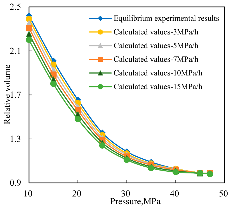
As depicted in Figure 23, the relative volume exhibits a monotonic increase as pressure decreases. When the pressure exceeds the dew point pressure, the system remains in a single-phase state, and changes in relative volume are negligible. However, once the pressure falls below the dew point, the differences among depletion rates become evident and progressively intensify as the pressure approaches the maximum retrograde condensation pressure. At any given pressure, the equilibrium curve consistently lies above all non-equilibrium curves; furthermore, the relative volume of the system is inversely related to the depletion rate. For example, at 10 MPa the relative volume is 2.42 at 3 MPa/h but only 2.20 at 15 MPa/h.

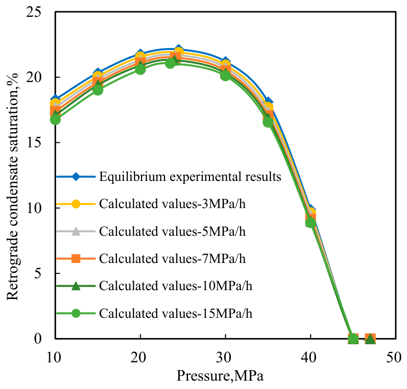
This deviation in relative volume directly translates into differences in retrograde condensate saturation (Figure 24). Across all depletion rates, condensate saturation exhibits similar phase transition trends, characterized by a sharp increase just below the dew point, followed by a deceleration or decline due to kinetic constraints and retrograde evaporation. At any given pressure, equilibrium saturation is consistently higher than non-equilibrium saturation, and the divergence becomes more pronounced at faster depletion rates. For example, at the maximum retrograde condensation pressure, equilibrium saturation reaches 22.12%, whereas at 15 MPa/h, it decreases to 21.05%. These results indicate that, at high depletion rates, the gas phase expands more rapidly than the liquid condensate can form, with a greater portion of the system’s free energy directed toward gas expansion. This behavior confirms that the depletion rate is a dominant factor governing non-equilibrium phase transitions, and it underscores the necessity of accounting for kinetic constraints when evaluating condensate behavior and predicting reservoir performance under varying production strategies.

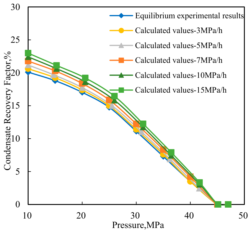
The combined effects of gas expansion and suppressed liquid formation ultimately influence the condensate recovery factor. As pressure depletes, the condensate recovery factor increases under both equilibrium and non-equilibrium conditions, but faster depletion consistently yields a higher recovery factor. At the abandonment pressure, the condensate recovery factor under equilibrium is 20.62%, whereas at 15 MPa/h, it reaches 22.98%, which is 2.36% higher. The underlying mechanism involves incomplete mass transfer and phase transitions at high depletion rates, which prevent the full condensation of heavy components. These heavy components are entrained by the high-velocity gas phase, while lighter components expand rapidly and partially dissolve into the liquid condensate. As a result, the condensate recovery factor is significantly enhanced at faster depletion rates, highlighting the critical role of non-equilibrium phase behavior in reservoir performance evaluation and production optimization (Figure 25).

5. Conclusions

This study develops a non-equilibrium dynamic phase transition model as a rate-dependent relaxation framework for describing kinetic deviations from thermodynamic equilibrium during pressure depletion. The model quantitatively relates the pressure depletion rate to relaxation kinetics during phase evolution and captures transient deviations from equilibrium under rapid depressurization. Although the governing framework is formulated in a general form for rate-sensitive oil–gas phase-transition processes, the analytical expression and optimized parameters reported in this work are calibrated and internally validated using the condensate-gas fluid investigated in this study. Therefore, the present validation should be interpreted as being specific to the studied condensate-gas system rather than as direct proof of universal applicability to all rate-sensitive reservoir fluids.

(1)

Model calibration and comparison with experimental data and tNavigator simulations demonstrate that the proposed approach reliably reproduces non-equilibrium phase behavior for the studied condensate-gas fluid, with average relative errors below 5%. Predictions at the hold-out depletion rates (7 and 15 MPa/h), which were not used for parameter calibration, agree well with experimental measurements. Faster depletion rates were found to prolong relaxation time and enhance non-equilibrium effects, indicating that rapid pressure decline suppresses interphase mass transfer and delays equilibrium attainment within the experimental conditions and fluid system considered in this work.

(2)

The model further reveals that the depletion rate strongly controls phase and production dynamics in the investigated gas-condensate system. With increasing depletion rates, relative volume and condensate saturation decrease, whereas the condensate recovery factor increases due to incomplete condensation and enhanced gas expansion. These findings describe the depletion rate-dependent response of the studied condensate-gas fluid and require further validation before being generalized to fluids with different compositions, condensate richness, or reservoir-temperature conditions.

(3)

Overall, the proposed model provides a theoretical basis for predicting non-equilibrium phase behavior under varying depletion conditions by coupling the external pressure-depletion timescale with the intrinsic phase-relaxation timescale. The governing framework may be transferable to other rate-sensitive hydrocarbon fluid systems; however, the optimized parameters α₀, kp, and n are fluid-specific and must be recalibrated before application to different fluids. In this study, the parameterized analytical expression was developed and internally validated using hold-out depletion-rate data from a single condensate-gas fluid dataset. Therefore, its current predictive applicability is limited to the studied condensate-gas fluid and comparable systems. Broader applicability to fluids with different compositions, temperatures, condensate richness, or to volatile-oil, black-oil, and gas-injection systems requires further validation.