A Unified Co-Optimization Framework for Hybrid Renewable Systems Incorporating Degradation-Aware Multi-Storage and Demand-Side Management

Abstract

The intermittent nature of renewable energy systems and the mismatch between power generation and load demand necessitate the integration of efficient energy storage systems (ESSs). Among large-scale energy storage technologies, pumped hydro-energy storage systems (PHESs) are widely recognized as one of the most cost-effective and longest-lifetime storage solutions under favorable geographical conditions. This study proposes and optimizes a hybrid renewable energy system (HRES) for the Wadi Baish region in Saudi Arabia as a real case study, where the significant elevation difference between the nearby mountains and the existing lake provides favorable conditions for PHES implementation. A nested optimization framework is developed to determine the optimal sizing and operation of the HRES components. The external optimization loop employs the non-dominated sorting genetic algorithm II (NSGA-II) to optimize system sizing, while the internal optimization loop uses mixed-integer linear programming (MILP) to optimally dispatch the PHES, battery energy storage system (BESS), and hydrogen energy storage system (HESS). In addition, demand-side management (DSM) is coordinated with the MILP dispatch strategy to improve system performance and reliability. The results show that the optimized system can supply a 10 MW average load with a renewable energy penetration of 98.7%. The proposed configuration achieves a total lifecycle cost of USD 231.37 million and avoids approximately 898.58 kt of CO₂ emissions over the project lifetime. PHES operates as the primary bulk energy storage technology due to its high storage capacity and low degradation characteristics. Furthermore, the degradation-aware model predicts battery replacement every 12 years and HESS replacement every 5 years. Compared with rule-based control, the MILP-based dispatch strategy reduces grid dependency by 87%. The coordinated DSM and MILP operation also reduces the levelized cost of energy to USD 0.066/kWh while improving overall system reliability. These findings demonstrate the importance of coordinated energy management and accurate degradation modeling in the optimal design and operation of renewable-based HRES configurations.

1. Introduction

1.1. Background

Modern power systems increase the penetration of renewable energy sources thanks to energy storage systems (ESSs) and demand-side management (DSM). Among the best ESSs, Pumped Hydro Energy Storage (PHES) remains the most mature and cost-effective for bulk storage, while lithium-ion batteries (LIBs) provide fast response, and hydrogen storage offers long-duration, seasonal capability and can be exported to some other projects. The Kingdom of Saudi Arabia, under Vision 2030 [1], is actively developing renewable energy projects, including the world-leading NEOM green hydrogen facility and several PHES projects [2,3].

Resolving these multi-faceted grid complexities demands a transition from traditional, isolated planning methods to a unified co-optimization framework. Designing a reliable HRES requires simultaneous balancing of long-term capital investments alongside short-term operational dynamics. This task becomes significantly more complex when managing a diverse, multi-storage portfolio. Each asset class exhibits fundamentally distinct response times, capital expenses, and degradation mechanisms. Ignoring these operational realities during the design phase leads to severely oversized systems or premature component failures. Therefore, a truly robust co-optimization framework must not only capture high-fidelity, degradation-aware lifetimes for multi-carrier storage, but it must also dynamically coordinate these assets with demand-side management (DSM) schemes to achieve optimal techno-economic performance.

Existing literature on HRES sizing often uses simplified storage degradation models (e.g., linear capacity fade independent of operating conditions) and metaheuristic dispatch rules [4,5,6]. More accurate degradation models consider depth of discharge (DoD), temperature, and cycle count available for batteries but are rarely used in sizing optimization algorithms [7,8,9,10]. Similarly, the degradation of the pump/turbine of the PHES due to cavitation and wear is usually ignored in sizing [2,3,11,12]. For hydrogen, performance decay is not treated as a function of the actual operation, but it is considered as a fixed lifetime rather than a function of operating hours and load cycles [13].

Moreover, DSM is implemented as a simple load shifting and ignores the different flexibility of different loads, such as the residential, agricultural, and industrial loads. Furthermore, the optimal dispatch of multi-storage systems is often solved by using rule-based heuristics or by linear programming (LP) without considering the binary variables (e.g., for startup/shutdown decisions), which leads to suboptimal results [14].

1.2. Literature Review

The increase in renewable energy systems in HRES necessitates ESSs and DSM strategies to enhance system reliability and stability. The integration of ESSs and DSM strategies in the operation of the HRES can remedy the effect of intermittency and enhance system stability [14,15]. However, considering these issues in the optimal sizing and operation makes it a very complex task due to the presence of stochastic natural resources and the stochastic behavior of the systems.

Various storage systems are considered a key to overcoming fluctuation problems in HRESs, with LIBs being among the most important. These batteries are characterized by their high efficiency and rapid charging and discharging response [8]. However, the problem of degradation in their lifecycle, such as decreased capacity and increased internal resistance, makes them more difficult to integrate into systems with optimal sizing, and therefore, many research studies do not take them into account. The degradation of LIBs is a function of the DoD, temperature, and current rate [16]. Several studies introduced accurate models of the degradation of LIBs but are still not widely used in modern sizing studies of HRESs [7,8,9,10].

The PHESs are widely used and have proven their effectiveness and feasibility in many projects and studies [2,3,11,12]. Its long lifespan and low cost per unit of stored energy, especially in sites with a high elevation difference, such as the Wadi Baish site. However, most existing studies assume constant efficiency and neglect cavitation, hydraulic losses, and mechanical wear [2,3,11,12,17]. The ignoring of such an important issue in the sizing problem can lead to inaccurate sizing of components, which can lead to reliability, stability problems, and techno-economic problems, especially when PHES plays a dominant role.

Hydrogen energy storage systems (HESS) have recently been considered as a complementary solution for long-duration and seasonal storage [13,18,19]. Through power-to-gas (P2G) conversion, excess renewable energy can be stored as hydrogen and later reconverted into electricity using fuel cells. While this approach enables sector coupling and high energy density storage, hydrogen systems are characterized by relatively low round-trip efficiency and high capital cost. Furthermore, degradation in electrolyzers and fuel cells driven by operating hours, load cycles, and material aging is often modeled using simplified lifetime assumptions rather than dynamic performance models [11,13,18,19,20].

Energy management (dispatch) methods play a significant role in the coordination of HRES operation. Rule-based heuristics are still extensively employed because of their simplicity [11,13,18,21] but usually lead to inferior performance, especially in systems with different storage technologies. Optimization-based techniques such as MILP and model predictive control (MPC) increase coordination by introducing system-wide restrictions and predictions [22]. But these techniques usually presume optimal behavior of the components and do not explicitly include degradation effects in the dispatch decisions.

Another form of flexibility is provided by DSM through changes in consumption patterns as a function of system circumstances. Although various studies show its ability to lower peak demand and boost renewable use [13,23,24,25,26], most approach demand in an aggregated manner or ignore it altogether [12,18,27]. Explicit modeling of the different flexibility characteristics of residential, agricultural and industrial loads is rarely done, limiting the accuracy of system-level evaluations.

To address the complexity of HRES design, a wide range of optimization techniques has been proposed. Deterministic approaches, especially LP [28] and MILP [23,24,25,26,29], are widely adopted due to their capacity to include system constraints and to provide optimal solutions for linear assumptions. Especially, MILP can be used to model discrete operational decisions such as unit commitment and storage mode switching. However, many MILP works utilize simplified models of the components and seldom include degradation dynamics or long-term variations in performance [22].

At the same time, metaheuristic algorithms such as genetic algorithm (GA) [21], particle swarm optimization (PSO) [24], grey wolf optimization (GWO) [23], musical chairs algorithm (MCA) [2,3], artificial rabbits optimization (ARO) [23], dragonfly algorithm (DA) [30], hybrid artificial gorilla troops optimizer with quadratic interpolation (HAGTO-QI) [21], firefly algorithm (FFA) [31], and non-dominated sorting genetic algorithm II (NSGA-II) have been widely utilized in HRES sizing problems [26]. These approaches are particularly suited for multi-objective optimization, allowing cost, emissions and reliability to be considered simultaneously. Recent research trends increasingly mix metaheuristic techniques for long-term sizing with deterministic-based methods (DBMs) [12,18] for short-term dispatch, establishing hybrid frameworks that balance the computational solution quality. However, most of the available studies assume static component properties, neglecting the cumulative effect of degradation on system performance and lifecycle cost [32].

In general, the current HRES studies tend to consider degradation, dispatch and demand flexibility in a disjointed manner, despite the significant improvements. This makes it difficult to capture the intricate interactions between system components and their changes throughout long-term operation.

1.3. Research Gap

The range of existing work is extensive, but there are still several fundamental limitations, as shown in the comparative analysis in

Table 1. Benchmarking of various HRES optimization studies, identifying key gaps in dispatch mathematical rigor, multi-storage degradation integration, and DSM synergy.

Ref.	System Components	Grid Connection	Optimization Method	Dispatch Modeling	Degradation Modeling	DSM Integration	Time Horizon	Key Performance
[13]	PV, wind, BESS, HESS	OFF Grid	NSGA-II and PSO	Rule-based	Limited	Strong	20	No optimal dispatch, weak degradation
[11]	PV, wind, BESS, HESS, PHES, thermal	ON Grid	PSO	Rule-based	Limited	Limited	25	No optimal dispatch
[18]	PV, wind, BESS, HESS	OFF Grid	DBM	Rule-based	Limited	None	25	Static operation
[30]	PV, wind, BESS, diesel	ON Grid	DA	Rule-based	Yes	Limited	20	No optimal dispatch, limited DSM
[21]	PV, wind, BESS, supercapacitor	ON Grid	HAGTO-QI	Rule-based	Limited	Limited	20	No optimal dispatch, limited DSM
[19]	PV, wind, BESS, HESS	ON Grid	GA-PSO	Rule-based	Limited	Limited	25
[12]	PV, wind, BESS, PHES	OFF Grid	GWO	Rule-based	Limited	Limited	20
[27]	PV, wind, BESS, biomass	OFF Grid	PSO	Rule-based	None	Limited	20	No optimal dispatch and degradation
[31]	PV, BESS, HESS	OFF Grid	FFA	Rule-based	Limited	Limited	Long-term	Weak temporal resolution
[23]	PV, wind, BESS, HESS	ON Grid	ARO	Fuzzy-Logic Battery Scheduling	Limited	Yes	20	High computational burden
[24]	PV, wind, BESS, HESS	ON Grid	PSO	MILP	Limited	Yes	25	High dimensional MILP complexity
[25]	PV, wind, BESS, HESS	ON Grid	Deterministic/multi-energy optimization	MILP	Limited	Yes	20	Limited experimental validation
[26]	PV, wind, BESS	ON Grid	NSGA-II	MILP	Yes	Yes	20	Substantial computational complexity
This Study	PV, Wind, BESS, PHES, HESS	ON Grid	NSGA-II	MILP+MPC	Yes	Yes	30 years	Fully integrated degradation-aware co-optimization of sizing, dispatch, and DSM

. A primary limitation is the absence of degradation-aware co-optimization of sizing and operation. In most studies, degradation is either neglected or treated as a fixed lifetime parameter. When considered, it is typically limited to battery systems and implemented in a simplified manner [13,18,19,21]. Even in the works that partially consider degradation [23,24,25,26,30], it is not treated consistently in both sizing and dispatch. Hence, operational decisions are not directly related to the long-term performance of components, leading to inaccuracies in lifecycle cost estimations.

Related to this is the lack of integrated multi-technology degradation modeling. There is no uniform representation of degradation for batteries, PHES and HESS in the existing studies. The effectiveness of PHES-based systems is usually assumed to be constant [11,12], whereas the lifespan of HESS is often assumed to be static [13,18,19]. Even sophisticated optimization frameworks [24,25,26] provide restricted degradation models, which are inadequate for a precise depiction of technology-specific aging mechanisms and their influence on system function.

Another important gap is the limited integration of DSM with the multi-storage coordination. Although DSM is considered in some research [13,23,24,25,26], it is often simplified or aggregated. Many works do not consider DSM at all [12,18,27], or do not distinguish between different load types [11,19,21,31]. Consequently, the interaction between flexible demand and heterogeneous storage technologies is not fully captured, reducing the effectiveness of coordinated energy management.

From a methodological perspective, dispatch modeling remains insufficiently rigorous or weakly coupled with system planning. A large portion of the literature relies on rule-based heuristics [11,13,18,21,27,31], which do not guarantee optimality. MILP-based approaches have also been investigated [24,25,26], but they tend to be computationally demanding or use simplified system models. In addition, the interconnection between dispatch optimization and system sizing is still limited, leading to an inconsistent evaluation of system performance.

Finally, long-term, high-resolution lifecycle evaluation is still underdeveloped. Several studies are constrained to short-term analyses [13,23,30], while others lack chronological optimization or temporal coupling [12,18,31]. Degradation and replacement dynamics are often simplified even for longer horizons, which does not accurately represent cumulative degradation effects and long-term system behavior. Moreover, the literature lacks a fully integrated framework that consistently incorporates degradation-aware optimization, multi-technology storage modeling, rigorous dispatch strategies and demand-side flexibility in a long-term planning and operational context. Filling these gaps requires a unified approach that explicitly captures the dynamic interactions among system components and their evolution over time.

1.4. Main Contributions

This study develops a unified optimization framework for the design and operation of HRES that explicitly captures the interactions between multi-technology storage, component degradation, and DSM over long-term planning horizons. The principal contributions are as follows:

• Degradation-aware co-optimization of sizing and dispatch.
• A novel integrated framework is proposed in which long-term component degradation is endogenously incorporated into both capacity sizing and short-term operational dispatch. Unlike conventional approaches that decouple planning and operation or assume static lifetimes, the proposed method dynamically updates component performance (capacity, efficiency, and operating limits) over a 30-year horizon, enabling more realistic lifecycle optimization.
• First comprehensive integration of multi-technology degradation within MILP dispatch.
• A MILP dispatch model is proposed that accounts for degradation effects in LIBs (capacity fade and resistance growth), PHES (efficiency decay with cumulative throughput) and HESS (electrolyzer and fuel cell performance degradation with operating hours) simultaneously. The linearization of degradation processes is embedded into the dispatch optimization so that the operational decisions reflect the long-term asset wear.
• Coupled modeling of DSM with multi-storage coordination.
• An advanced DSM formulation is developed and co-optimized with supply-side resources. The model distinguishes residential, agricultural and industrial loads with different flexibility characteristics, e.g., price-responsive shifting and interruptible demand. The framework allows for capturing system-level interactions between flexible demand and heterogeneous storage technologies.
• Multi-objective planning under realistic operational constraints.
• A multi-objective optimization model based on NSGA-II is formulated to simultaneously minimize lifecycle cost, CO₂ emissions, and grid dependency. The framework embeds a rolling-horizon MILP dispatch within each candidate solution, ensuring that sizing decisions are evaluated under operationally optimal and constraint-consistent conditions.
• Application to a high-head PHES-integrated hybrid system with site-specific accuracy.

The case study used to demonstrate the suggested framework is the Wadi Baish area in Saudi Arabia, where a substantial topographic potential for high-head PHES exists. The case study presents site-specific renewable resources, load segmentation, and realistic infrastructure assumptions and proves the feasibility and strategic usefulness of integrating PHES with complementary storage technologies in dry, high-irradiance locations.

Although the Wadi Baish area is used as a representative case study, the proposed degradation-aware optimization framework is not site-specific and can be generalized to other high-head PHES-integrated hybrid renewable energy systems. The combined NSGA-II/MILP framework with coordinated DSM and multi-storage degradation modeling can be applied to mountainous regions with suitable elevation differences and renewable resources.

1.5. Study Outlines

The remainder of this paper is organized into seven subsequent sections. Section 2 describes the study site at Wadi Baish, featuring high-head pumped hydro potential and multi-sector load profiles. Section 3 introduces advanced component modeling, including physics-informed degradation for batteries, pumped hydro and hydrogen systems. Section 4 presents the operational framework, consisting of a rolling-horizon MILP dispatch formulation considering component wear. Section 5 presents the multi-objective optimization process for system sizing coupled with price-based demand-side management (DSM) using the NSGA-II algorithm. Section 6 discusses the results, including a comparison between the MILP dispatch and traditional heuristics and an analysis of the impact of demand flexibility. Moreover, Section 6 presents a sensitivity analysis and a discussion on strategic implications for energy policy. Section 7 concludes the paper with a summary of main research contributions and prospects for future research on degradation-aware renewable systems.

2. Site Description

2.1. Location and Climate

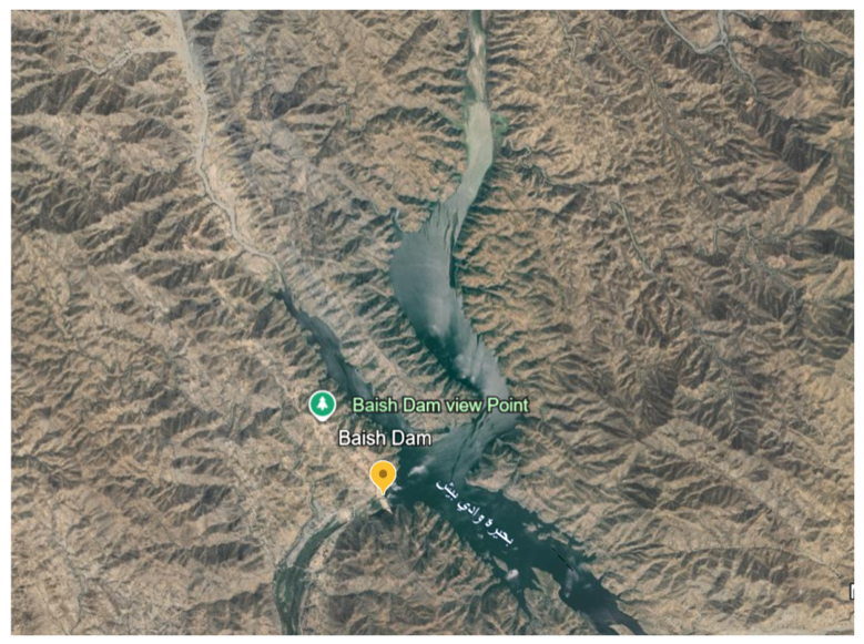
Wadi Baish is located in the Jazan region of southwestern Saudi Arabia (approximately 17° N, 43° E). The area has a hot desert climate with substantial solar irradiation. The characteristics of the site from Google Earth are shown in Figure 1. The Jazan region has a Global Horizontal Irradiance (GHI) of about 2300 kWh/m²/year, one of the highest in the world [33]. Average annual wind speed at 100 m hub height is about 4.5–5.0 m/s [33], moderate but suitable for wind energy, especially if the wind turbines are installed at the top of the mountains.

Wadi Baish is a strategically significant location for PHES due to three factors: (1) an existing dam (completed 2017) that serves as a lower reservoir, eliminating major civil works; (2) a 1800 m hydraulic head from the dam to the Al Gabal Al Asoad mountain, which would be among the highest in the world (surpassing the Bieudron plant’s 1703 m record); and (3) the presence of residential, agricultural, and industrial loads within 30 km, providing a realistic demand profile. While the methodological contributions are general, the case study demonstrates the framework’s applicability to a real-world high-head PHES site.

2.2. PHES Potential Using Wadi Baish Dam

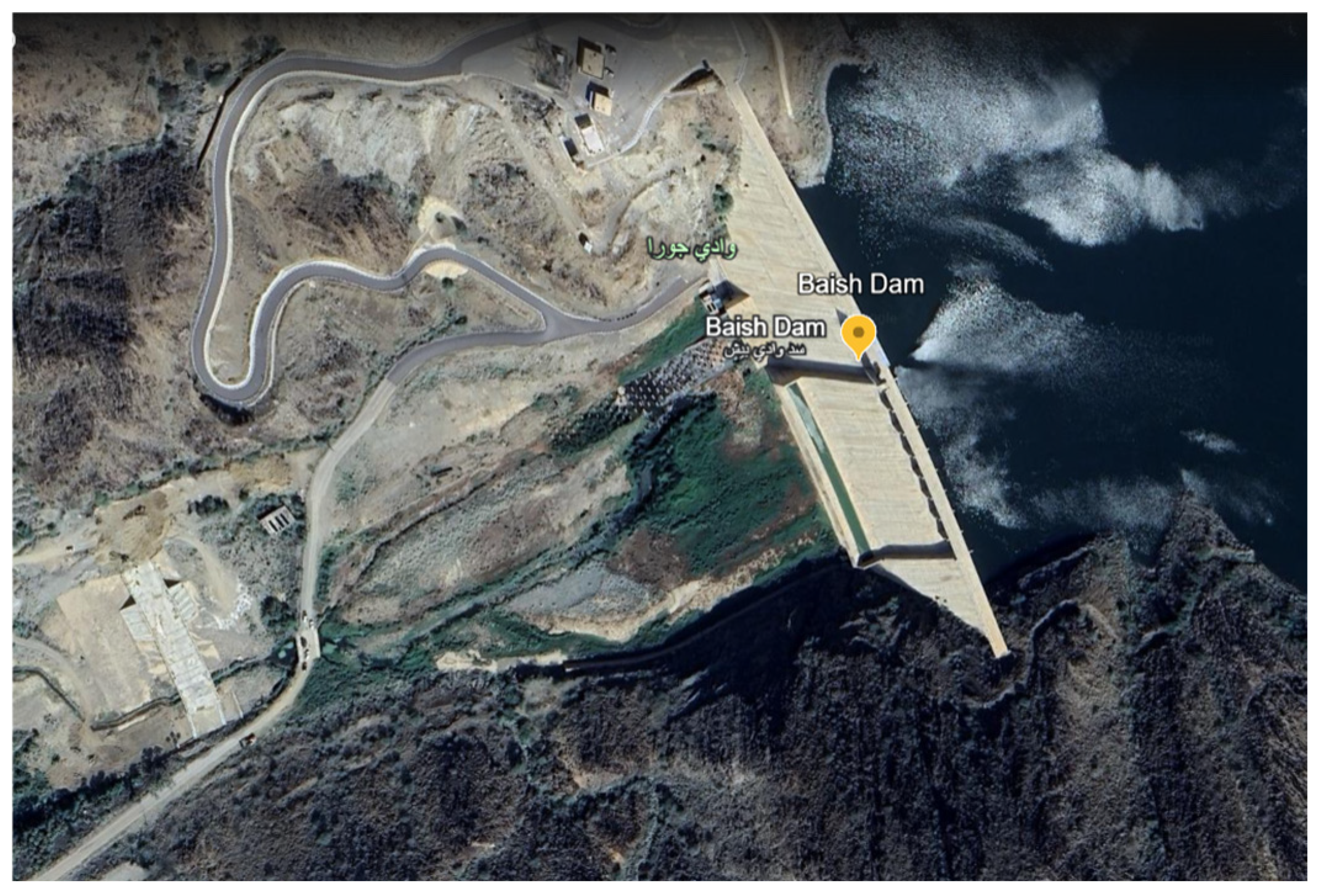
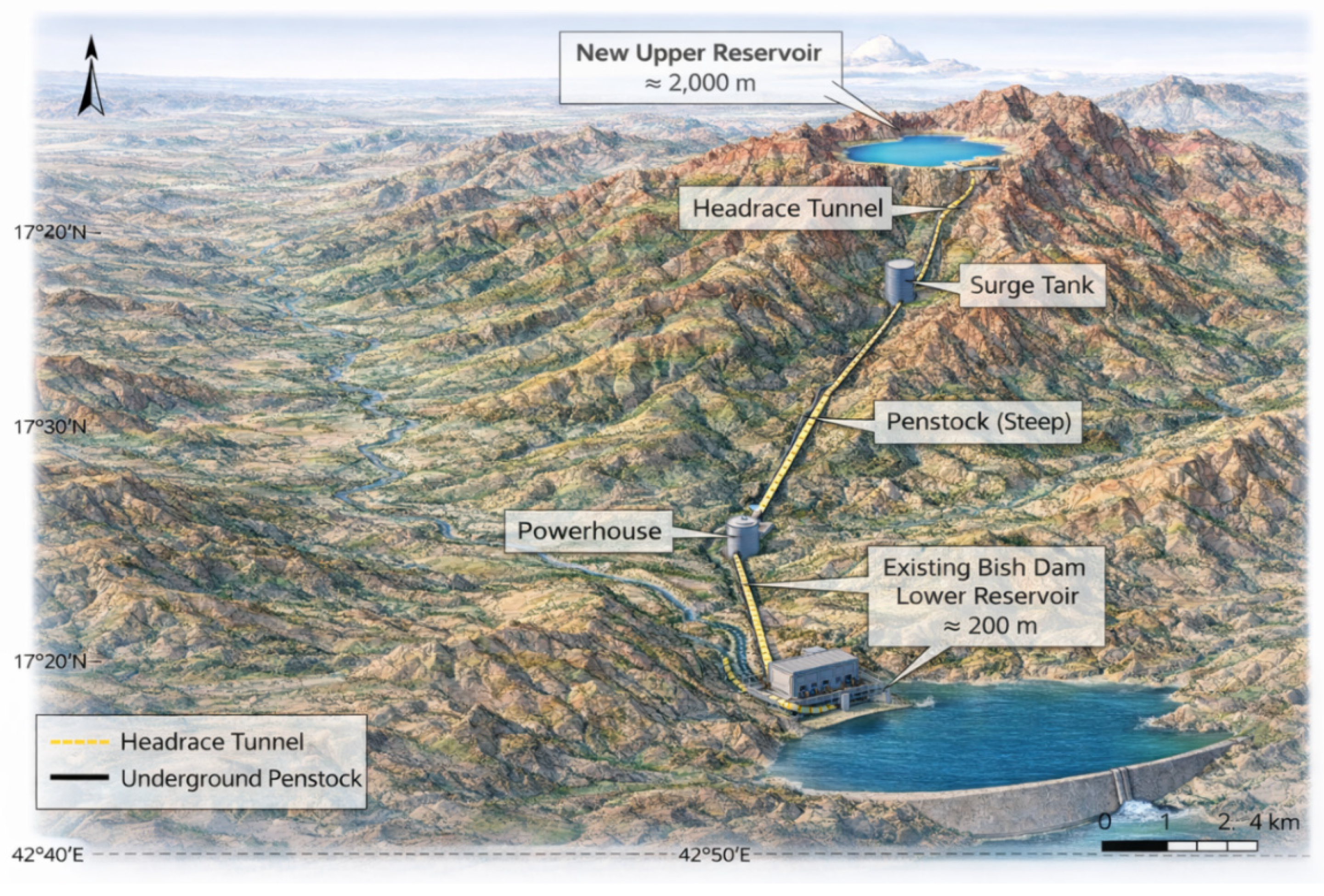
The existing Wadi Baish Dam (completed in 2017) is an earth-fill dam with a height of 70 m and a storage capacity of 10 million cubic meters, as shown in Figure 2 [34]. The dam currently serves irrigation and flood control. For PHES, the dam can be used as the lower reservoir. The upper reservoir would be constructed on the nearby Al Gabal Al Asoad mountain (elevation ~2200 m), approximately 12 km from the dam. The effective head is estimated at 1800 m [34,35]. Effective head would make this one of the highest-pressure PHESs in the world (surpassing the world-record Bieudron plant at 1703 m) [36]. The maximum power capacity from a PHES plant in terms of head, h, and flow rate, Q, is obtained from Equation (1). The theoretical potential energy stored is governed by Equation (2). These equations are used to estimate the upper bound of PHES capacity at the Wadi Baish site.

$$P_{PHES,\max }=\eta \cdot \rho \cdot g\cdot h\cdot Q$$

(1)

The theoretical potential energy stored in a PHES system is governed by

$$E=\rho \cdot g\cdot h\cdot V$$

(2)

where E is the stored energy (J), ρ is water density (kg/m³), g is the gravitational acceleration (m/s²), h is the hydraulic head (m), and V is the active storage volume (m³).

2.3. Hydraulic Considerations

The hydraulic design of the proposed PHES system is of crucial importance to its overall efficiency, reliability and long-term performance. The substantial hydraulic head at the Wadi Baish site requires particular consideration of hydraulic loss minimization and system stability during dynamic operating conditions.

A key consideration is friction loss minimization within the headrace tunnels and penstocks. These losses due to viscous effects and internal surface roughness can lead to significant reduction in net head and, hence, energy conversion efficiency of the system. The tunnel and penstock diameters are carefully optimized to strike a compromise between hydraulic efficiency and capital cost. The increase in diameter results in a decrease in the flow velocity and frictional head loss but also in an increase in excavation costs and material costs. Then, a techno-economic trade-off is carried out to find the optimal design that minimizes energy losses without excessive construction costs.

Transient hydraulic effects like water hammer are also handled as an important feature. Pressure surges, which can damage pipelines and mechanical components, can be generated by abrupt changes in flow conditions, such as sudden load rejection or switching between pump and turbine operation. To prevent this, a surge tank is added to the system design that serves as a hydraulic accumulator to absorb the excess pressures during transient events and to allow stable flow conditions. A detailed system dynamic analysis is presented to establish the location and size of the surge tank to mitigate the pressure fluctuations efficiently without deteriorating the system flexibility.

For high-head PHESs, the choice of suitable turbine technology is also critical. Considering the high elevation difference in the site, high-head turbines such as Pelton or high-head Francis turbines are recommended [37]. Pelton turbines are well suited for substantial head low flow situations, with high efficiency and rugged performance. For other situations, high-head Francis turbines allow for more operational flexibility under varying flow conditions and are useful when a greater operational window is desired. The final selection is based on detailed hydraulic analysis, projected operational profiles and economic evaluation to optimize energy conversion efficiency over a range of operational states.

A surge tank is included in the hydraulic design to mitigate pressure transients during rapid load changes. Detailed transient simulation of water hammer effects is beyond the scope of this paper; the surge tank sizing is based on standard engineering guidelines [36]. A comprehensive hydraulic transient analysis is left for future work.

2.4. Design Significance

The proposed PHES system in Wadi Baish has several strategic advantages that improve the technical and economic feasibility of the system in an HRES. The system has a substantial energy density due to the large hydraulic head available between the upper and lower reservoirs. The energy storage capacity of PHES is proportional to the water volume and the elevation difference; hence, the large head at this site enables a large amount of energy to be stored with relatively small reservoir volumes. This leads to a compact but very efficient storage system compared to conventional low-head systems, increasing the efficiency of land use and improving the overall system performance.

In addition, the design leverages the natural topography of the region to achieve reduced civil construction costs. The existing terrain features, such as the Wadi Baish Dam as the lower reservoir and the adjacent mountainous elevations for the upper reservoir, are used to minimize the need for extensive excavation and large-scale structural works. This terrain-oriented design approach not only reduces the capital expenditure but also minimizes the environmental impact, making the system sustainable and easier to implement.

3. Component Models and Degradation

3.1. Solar PV

PV power output is modeled using the single-diode model with temperature correction. No additional degradation beyond the warranty-based linear fade (0.5% per year) is applied; PV panels are replaced at year 25.

The power output at hour t is [38]

$$P_{pv}\left(t\right)=G\left(t\right)\cdot A_{pv}\cdot {\eta }_{pv}\left(t\right)$$

(3)

where G(t) is global horizontal irradiance (W/m²), $A=P_{pv,rated}/\left(G_{STC}\cdot {\eta }_{STC}\right)$ is the array area, and PV efficiency can be obtained from

$${\eta }_{pv}\left(t\right)={\eta }_{STC}\left[1+{\beta }_T\left(T_{cell}\left(t\right)-T_{STC}\right)\right]$$

(4)

where cell temperature is

$$T_{cell}\left(t\right)=T_{amb}\left(t\right)+\left(G\left(t\right)/1000\right)$$

(5)

where G(t) is the global horizontal irradiance at time step t, A_pv is the total active surface area of the PV array in m², ${\eta }_{\mathrm{PV}}\left(t\right)$ is the effective PV conversion efficiency at time t, accounting for temperature and degradation, ${\eta }_{STC}$ is the reference efficiency of the PV module at standard test conditions (STC), b is temperature coefficient of power (efficiency loss per °C), and T_STC is the reference temperature at STC (typically 25 °C).

3.2. Wind Turbine

The power curve of the wind turbine is represented as shown in Equation (6). Degradation of wind turbines is modeled as a reduction in capacity factor by 0.2% per year due to blade erosion and mechanical wear [39].

$$P_{wt}\left(v\right)=\left\{\begin{array}{cc}0& v<v_{ci}\\ P_{rated}{\left({\displaystyle \frac{v-v_{ci}}{v_r-v_{ci}}}\right)}^3& v_{ci}\le v<v_r\\ P_{rated}& v_r\le v\le v_{co}\\ 0& v>v_{co}\end{array}\right.$$

(6)

where v_ci is the cut-in speed, v_r is the rated wind speed, v_co is the cut-out wind speed, and P_rated is the power of the wind energy system.

3.3. Lithium-Ion Battery Advanced Degradation

A semi-empirical capacity fade model was implemented, following the methodology in [16] for hot climates such as Jazan, where capacity loss ΔC is a function of DoD, number of cycles N, and temperature T, as shown in Equation (7). The parameters ‘E_a = 35,000 J/mol’ and the pre-exponential factor ‘A = 2946’ are calibrated to laboratory cycling data at 30 °C. This model was selected because it captures the two dominant degradation mechanisms: cycle-induced capacity loss (∝ √N) and temperature acceleration (Arrhenius), while remaining computationally tractable for integration with MILP.

$$\Delta C_o=A\cdot N^{0.5}\cdot e^{\left(-{\displaystyle \frac{E_a}{RT}}\right)}\cdot Do{D}^{1.2}$$

(7)

where A is a pre-exponential factor, E_a = 35,000 J/mol (activation energy), R is the gas constant and equal to 8.314 J/(mol⋅K), and T is measured in Kelvin. The real temperature for Jazan is considered to calculate the accurate degradation, giving a temperature factor.

For each cycle in the dispatch, the DoD is computed, and the cumulative capacity loss is updated using a rainflow counting algorithm (implemented in the code). Additionally, internal resistance increase is modeled as [40]

$$R\left(t\right)=R_0\left(1+k_R\cdot N^{0.8}\right)$$

(8)

With k_R calibrated to double resistance after 5000 cycles [40]. This affects efficiency slightly.

The battery’s calendar degradation is a function of the SoC, temperature and unused time, which can be obtained as the following [10]:

$$\Delta C_s=A_1\cdot e^{\left(B_1\cdot SoC-\left(E_a+C_1\cdot SoC\right)/RT\right)}\cdot t^{D1}$$

(9)

The parameters A₁ to D₁ can be obtained from the calendar test [10]. The values of these parameters have been used as the values introduced in [10].

3.4. PHES Efficiency Degradation

PHES efficiency degrades due to cavitation, erosion, and wear of pump/turbine runners. The pump efficiency η_pump(t) and turbine efficiency η_turb(t) are modeled as follows [20]:

$$\eta \left(t\right)={\eta }_0\cdot e^{\left(-\lambda \cdot E_{throughput}\right)}$$

(10)

where E_throughput is the cumulative energy passed through the component (MWh), and λ is a decay constant chosen such that efficiency drops by 0.25% every year (typical for large PHES) [20]. The round-trip efficiency thus declines from 0.85 × 0.85 = 0.7225 to about 0.775 × 0.775 = 0.6 after 30 years of heavy use [41]. Replacement of pump/turbine runners occurs when efficiency drops below 0.75 of the initial (about 25% degradation), which is computed from the simulated throughput [42].

The degradation parameters for PHES are derived from Zhao et al. [20], who conducted experimental cavitation tests on pump-turbine runners. The decay constant “λ = −ln(0.9)/10,000” corresponds to a 10% efficiency drop after 10,000 MWh throughput, which is typical for large-scale PHESs [41].

3.5. Hydrogen Storage Degradation

3.5.1. Electrolyzer Degradation

The primary degradation mechanism is membrane thinning and catalyst dissolution, leading to increased voltage at constant current. This is represented as an increase in specific energy consumption (kWh/kg H₂) over time [43],

$$E_{el}\left(t\right)=E_{el,0}\cdot \left(1+B_{el}\cdot H_{op}\right)$$

(11)

where H_op is cumulative operating hours (thousands), and β_el = 0.01 per 1000 h (1% increase per 1000 h). After 8000 h (≈1 year of continuous operation, but electrolyzers in hybrid systems operate intermittently), efficiency drops by 16%. Replacement is triggered when energy consumption increases by 30% [44,45].

3.5.2. Fuel Cell Degradation

The voltage decay leads to lower power output at constant hydrogen flow. The power output degradation can be modeled as follows [46]:

$$P_{fc}\left(t\right)=P_{fc,0}\cdot \left(1-{\gamma }_{fc}\cdot H_{op}\right)$$

(12)

with γ_fc = 0.01 per 1000 h. Replacement when power drops to 70% of nominal.

3.5.3. Hydrogen Storage Tank Degradation

Hydrogen storage tank degradation is considered lossless with no degradation. No self-discharge is considered, but the compressor consumes 0.5% of stored energy per day for maintaining pressure (included as a constant load) [46].

4. Optimal Dispatch via MILP

In a HRES with multiple storage technologies (BESS, PHES, and HESS), the dispatch algorithm determines how much power flows between each component at every time step. The choice of dispatch strategy has a profound impact on system performance, component lifetime, and overall cost. Conventional approaches include the rule-based heuristics [13,18] and continuous LP [14]. Rule-based heuristics (e.g., “discharge battery first, then PHES, then hydrogen”) [13,18]. The simple pseudo-code of the rule-based dispatch is shown below:

For each hour t:     net = load(t) − (PV(t) + wind(t))     If net > 0: // deficit         remaining = net         discharge battery → PHES → hydrogen → grid import     Else:        // excess         remaining = -net         charge battery → PHES → hydrogen → curtail Pch/dis = min(remaining, Pmax, ΔSoC × Enom/Δt) % Pch/dis is discharge/charge power.

These are simple and fast, but they cannot optimize across multiple storage devices with different efficiencies, degradation characteristics, and operational constraints. Moreover, LP can handle efficiency and power limits but cannot represent discrete decisions such as turning an electrolyzer ON/OFF (which has a minimum power requirement) or selecting the operation mode of a pumped hydro plant (pumping, turbining, or idle).

MILP overcomes these limitations of RBH and LP by introducing binary (0/1) variables. It can simultaneously optimize continuous power flows and discrete operating modes over a finite horizon, making it the preferred method for optimal dispatch in complex HRES. In practice, the LP approximation often gives results close to the MILP because simultaneous pumping and turbining are rarely optimal given efficiencies. However, for electrolyzers and fuel cells, ignoring minimum power can lead to unrealistic operation (e.g., running at 1% power, which is inefficient or impossible). Therefore, the full MILP is recommended for high-fidelity studies.

To manage the computational complexity of a full one-year (8760 h) planning horizon as a single MILP, the problem is addressed using a rolling horizon or MPC framework [22] as shown in the following steps:

• At each decision hour (t), obtain forecasts of load, PV generation, and wind generation for the next (τ) hours (typically (τ = 24)).
• Formulate and solve the MILP for these (τ) hours, obtaining optimal values for all decision variables (powers, states, binary modes) for the entire horizon.
• Apply only the first hour’s decisions (the “control move”) to the real system.
• Update the physical states (e.g., SoC, degradation counters) based on the applied actions.
• Move the horizon one hour forward (i.e., (t → t + 1)) and repeat.

This approach offers a compromise between optimality (by looking ahead 24 h) and computational tractability. Setting τ = 24 enables us to capture the daily pattern of solar radiation and load, while keeping the size of the MILP tractable.

4.1. Mathematical Formulation

4.1.1. Time Discretization

Let the dispatch horizon consist of (τ) time steps, each of duration (Δt) (here (Δt = 1) hour). Indices (t = 1, 2, …, τ) denote steps within the horizon. All quantities are assumed constant over each hour.

4.1.2. Decision Variables

The continuous (real) variables are as follows:

• P_grid(t) ≥ 0—power imported from the grid (kW). No export is allowed.
• P_curt(t) ≥ 0—power curtailed from renewable sources (kW).
• P_bat,ch ≥ 0, P_bat,dis ≥ 0—battery charging and discharging power (kW). They cannot be positive simultaneously because that would represent a loss; the MILP will naturally avoid this due to efficiency penalties.
• P_phes,pump(t) ≥ 0, (P_phes,turb(t) ≥ 0—PHES pumping (charging) and turbining (discharging) power (kW). These are also mutually exclusive via binary constraints.
• P_el(t) ≥ 0, P_fc(t) ≥ 0—electrolyzer and fuel cell power (kW).
• SoC_bat(t), SoC_phes(t), SoC_h2(t)—state of charge of each storage, dimensionless between 0 and 1.

Binary (integer) variables are shown in the following points:

• u_el(t) ϵ {0,1}—electrolyzer ON/OFF. When ON, the electrolyzer power must be between a minimum and maximum.
• u_fc(t) ϵ {0,1}—fuel cell ON/OFF.
• u_pump(t) ϵ {0,1}, u_turb(t) ϵ {0,1}—PHES operation mode. They are mutually exclusive: u_pump(t) + u_turb(t) ≤ 1. When both are zero, the PHES is idle.

4.2. Objective Function for MILP

The objective of the MILP is to minimize the total operational cost over the horizon, which is dominated by grid import. Additionally, small penalties are added to encourage the use of renewable energy and to avoid unnecessary storage cycling. The exact form of MILP objectives is shown in Equation (13). This quadratic penalty discourages the MILP from artificially depleting or overfilling storage at the horizon boundary.

$$\min {\displaystyle \sum _{t=1}^{\tau }\left[\begin{array}{l}{c}_{grid}\left(t\right)\cdot P_{grid}\left(t\right)\cdot \Delta t+{\epsilon }_{curt}\cdot P_{curt}\left(t\right)\cdot \Delta t+{\epsilon }_{SoC}.{\displaystyle \sum \left\{i\in \left(bat,phes,h2\right)\right\}{\left(So{C}_{\mathrm{target}}-So{C}_i\left(\tau \right)\right)}^2}\\ +{\epsilon }_{cycle}\left(P_{bat,ch}\left(t\right)+P_{bat,dis}\left(t\right)+P_{phes,pump}\left(t\right)+P_{phes,turb}\left(t\right)+P_{el}\left(t\right)+P_{fc}\left(t\right)\right)\Delta t\end{array}\right]}$$

(13)

where c_grid(t) is the time-varying electricity price. ε_curt is a small positive constant (e.g., 0.001) to prioritize storing excess energy over curtailment. ε_cycle is an even smaller constant (e.g., 0.0001) to break ties and slightly discourage unnecessary cycling; the actual degradation cost is handled in the outer optimization. ε_SOC = 0.001 and SOC_target = 0.5 is the target state of charge at the end of the horizon.

In the multi-objective sizing framework, the dispatch MILP does not directly include emissions or long-term degradation costs; those are accounted for in the outer NSGA-II optimization. The dispatch simply minimizes short-term operational costs with the given component sizes and efficiencies.

The rainflow counting algorithm, which accurately tracks battery cycles based on DoD, is executed only in the outer NSGA-II loop during the yearly degradation update. Inside the MILP dispatch, a linear proxy is used to maintain linearity: $\Delta N={\displaystyle \frac{(P_{ch}+P_{dis})\times \Delta t}{2.E_{nom}}}$. This approximation is acceptable because the MILP horizon is only 24 h, and the linear proxy correlates well with the rainflow count over short periods, as validated in [10].

4.3. Constraints

4.3.1. Power Balance (Equality)

At every hour, the sum of generated power plus imported power plus discharged storage must equal the load plus curtailed power plus charged storage:

$$\begin{array}{l}{P}_{pv}\left(t\right)+P_{wind}\left(t\right)+P_{grid}\left(t\right)+P_{bat,dis}\left(t\right)+P_{phes,turb}\left(t\right)+P_{fc}\left(t\right)\\ =P_{load}\left(t\right)+P_{curt}\left(t\right)+P_{bat,ch}\left(t\right)+P_{phes,pump}\left(t\right)+P_{el}\left(t\right)\end{array}$$

(14)

This constraint ensures energy conservation and is linear in all variables.

4.3.2. Storage Dynamics

Each storage device evolves according to its energy balance, accounting for round-trip efficiencies as shown in the following points [47,48]:

Battery:

$$So{C}_{bat}\left(t+1\right)=So{C}_{bat}\left(t\right)+{\displaystyle \frac{{\eta }_{bat,ch}\cdot P_{bat,ch}\left(t\right)\cdot \Delta t}{E_{bat,nom}}}-{\displaystyle \frac{P_{bat,dis}\left(t\right)\cdot \Delta t}{{\eta }_{bat,dis}\cdot E_{bat,nom}}}$$

(15)

PHES:

$$So{C}_{phes}\left(t+1\right)=So{C}_{phes}\left(t\right)+{\displaystyle \frac{{\eta }_{pump}\cdot P_{phes,pump}\left(t\right)\cdot \Delta t}{E_{phes,nom}}}-{\displaystyle \frac{P_{phes,turb}\left(t\right)\cdot \Delta t}{{\eta }_{turb}\cdot E_{phes,nom}}}-{\eta }_{evap}.\Delta t$$

(16)

Hydrogen:

$$So{C}_{h2}\left(t+1\right)=So{C}_{h2}\left(t\right)+{\displaystyle \frac{{\eta }_{el}\cdot P_{el}\left(t\right)\cdot \Delta t}{E_{h2,nom}}}-{\displaystyle \frac{P_{fc}\left(t\right)\cdot \Delta t}{{\eta }_{fc}\cdot E_{h2,nom}}}$$

(17)

where E_nom denotes the nominal energy capacity (kWh). Note that for hydrogen, the SoC represents the fraction of stored hydrogen energy equivalent. η_evap = 0.001 per day (0.1% daily evaporation loss from the reservoirs, as estimated from climate data for the Jazan region [33]).

4.3.3. State-of-Charge Limits

The SoC of each ESS should be within the allowable limits as follows:

$$So{C}_{\min }^i\le So{C}_i\left(t\right)\le So{C}_{\max }^i,\hspace{1em}\hspace{1em}\hspace{1em}i\in \left\{bat,phes,h_2\right\}$$

(18)

where $So{C}_{\min }^i$ and $So{C}_{\max }^i$ are the minimum and maximum SoC of the ESS components.

These limits protect the storage from deep discharge or overcharge, which accelerates degradation. Typical values: battery 0.2–1.0, PHES 0.1–1.0, hydrogen 0.1–1.0.

4.3.4. Power Limits

-

Grid import: $0\le P_{grid}\left(t\right)\le P_{grid,\max }$ (in practice, $P_{grid,\max }$ is set to a large number, e.g., 100 MW, as the grid is assumed unlimited) [49].

-

Curtailment: $0\le P_{curt}\left(t\right)\le P_{pv}\left(t\right)+P_{wind}\left(t\right)$

-

Battery: $0\le P_{bat,ch}\left(t\right)\le P_{bat,\max }$, $0\le P_{bat,dis}\left(t\right)\le P_{bat,\max }$

-

PHES: $0\le P_{bat,pump}\left(t\right)\le P_{phes,\max }$, $0\le P_{bat,turb}\left(t\right)\le P_{phes,\max }$

-

Electrolyzer and fuel cell: $0\le P_{el}\left(t\right)\le P_{el,nom}$, $0\le P_{fc}\left(t\right)\le P_{fc,nom}$

4.3.5. Minimum Power and Binary Logic for Electrolyzer/Fuel Cell

Electrolyzers and fuel cells cannot operate efficiently at arbitrarily low power. A minimum power threshold (typically 20% of nominal) is required. This is modeled using binary variables:

Electrolyzer: $P_{el}\left(t\right)\ge P_{el,\min }\cdot u_{el}\left(t\right)$, $P_{el}\left(t\right)\le P_{el,nom}\cdot u_{el}\left(t\right)$

Fuel cell: $P_{fc}\left(t\right)\ge P_{fc,\min }\cdot u_{fc}\left(t\right)$, $P_{fc}\left(t\right)\le P_{fc,nom}\cdot u_{fc}\left(t\right)$

When the binary variable is 0, the power is forced to zero. When it is 1, the power is between the minimum and maximum.

4.3.6. PHES Mode Exclusivity

The PHES cannot pump and turbine simultaneously. This is enforced by:

$$u_{pump}\left(t\right)+u_{turb}\left(t\right)\le 1$$

(19)

$$P_{phes,pump}\left(t\right)\le P_{phes,\max }\cdot u_{pump}\left(t\right)$$

(20)

$$P_{phes,turb}\left(t\right)\le P_{phes,\max }\cdot u_{turb}\left(t\right)$$

(21)

If both binaries are 0, the PHES is idle; if u_pump = 1 then only pumping is allowed; if u_turb = 1 then only turbining is allowed.

4.3.7. Ramping Constraints

To avoid unrealistic instantaneous changes in power (e.g., battery charging at full power one hour and discharging at full power the next), ramping limits can be added. For example,

$$\left|P_{bat,ch}\left(t\right)-P_{bat,ch}\left(t-1\right)\right|\le \Delta P_{bat,ramp}$$

(22)

Similar constraints are applied to all power variables. These are linear if expressed as two inequalities. However, they increase problem size and are often omitted in hourly dispatch models because the time step is already coarse.

4.4. Initial and Terminal Conditions

To ensure consistency between successive windows, the initial SoC of each storage at the start of the horizon is set to the actual SoC from the previous hour. No specific terminal condition is enforced (the horizon is short enough that end-of-horizon SoC does not significantly affect long-term behavior). However, to avoid “end-of-horizon effects” (e.g., emptying storage at the end of the forecast window), a small penalty on deviations from a target SoC (e.g., 50%) can be added to the objective.

4.5. Implementation Details

4.5.1. Problem Size

For τ = 24 h, the numbers of variables and constraints are as follows:

-

Continuous variables: 8 τ + 3(τ +1) = 11 τ + 3 = 267 (for (τ =24)).

-

Binary variables: 4 τ = 96 (electrolyzer ON/OFF, fuel cell ON/OFF, pump mode, and turbine mode per hour).

-

Equality constraints: τ (power balance) + 3 τ (storage dynamics) + 3 (initial SoC) =4 τ +3 = 99.

-

Inequality constraints: 2 × 3 τ (SoC limits) + various power bounds and binary logic constraints, totaling about 200.

This is a moderate-sized MILP that can be solved in a few milliseconds using a good solver such as MATLAB’s ‘intlinprog’. For a full year with 8760 h, the rolling horizon requires 8760 solves, which is computationally heavy but feasible with parallelization (e.g., solving each window independently after receiving forecasts).

4.5.2. Solver Selection

MATLAB’s ‘intlinprog’ is suitable for small to medium MILPs. For faster performance, Gurobi or CPLEX can be used via the MATLAB interface. In the provided code, an LP approximation (without binary variables) was used for demonstration, but the full MILP is described here.

4.5.3. Integration with the Outer Sizing Optimization

The MILP dispatch is embedded inside the objective function of the multi-objective sizing optimization (NSGA-II). For each candidate set of component sizes (PV, wind, BESS, PHES, HESS), the system over the 30-year project lifetime is simulated as follows:

• For each year, run the rolling-horizon MILP dispatch using the current component capacities and efficiencies.
• Record the grid import, storage cycles, and operating hours.
• Degradation parameters (capacity fade, efficiency loss) update, replacements triggered if thresholds exceeded.
• Accumulate discounted costs and emissions.

This nested approach is computationally expensive but yields highly accurate lifecycle cost estimates that reflect realistic dispatch strategies. Without MILP, rule-based heuristics may overestimate grid import and thus bias the sizing toward larger storage.

Higher temporal resolution (e.g., 15 min) would better capture sub-hourly variability and ramping events. However, for a 30-year simulation with a rolling-horizon MILP, 15 min resolution would increase the number of MILP solves from 8760 to 35,040 per year (a factor of 4), making the optimization computationally prohibitive (estimated wall-time > 6 months). This is a clear direction for future work, possibly using surrogate modeling or parallel computing. The present 1 h resolution is standard in long-term HRES sizing studies [13,18,19].

The decision variables used with the MILP (Continuous and binary) are shown in

Table 2. The decision variables used with the MILP.

Continuous Decision Variables		Binary Decision Variables
Name	Symbol	Name	Symbol
battery charge/discharge	Pbat,ch(t), Pbat,dis(t)	PHES pump mode	upump(t) ∈ {0,1}
PHES pump/turbine	Pphes,pump(t), Pphes,turb(t)	PHES turbine mode	uturb(t) ∈ {0,1}
electrolyser and fuel cell power	Pel(t), Pfc(t)	electrolyzer ON/OFF (minimum power 20% of rating)	uel(t) ∈ {0,1}
state of charge	SoCbat(t), SoCphes(t), SoCh2(t)	fuel cell ON/OFF	ufc(t) ∈ {0,1}
power imported from grid (≥0, no export allowed)	Pgrid(t)	curtailed renewable power	Pcurt(t)

.

The objective (per time step, within rolling horizon) is to minimize the weighted sum of grid import cost, degradation cost (BESS, PHES, HESS) approximated as linear functions of throughput and cycles, and load shedding penalty. Degradation cost coefficients are pre-computed from long-term models, e.g., battery cycle cost equals replacement cost/lifespan. Rainflow is used in outer simulation; meanwhile, a linear proxy is used inside MILP only.

5. Sizing Methodology

5.1. Demand-Side Management (DSM)

A price-based DSM is implemented using a day-ahead dynamic pricing signal for consumers only. The actual cost of grid import to the system operator remains constant. The time-of-use rates are used to incentivize consumer load shifting. Consumers respond by shifting flexible loads. The elasticity of different loads is summarized in the following points:

Residential loads: Each household has 30% of its consumption (dishwasher, EV charging, water heating) shiftable within a 6 h window. The DSM optimization minimizes total cost to consumers given the price signal.

Agricultural irrigation: Irrigation pumps can be scheduled flexibly as long as the daily water requirement is met. We model a total daily energy requirement of 12 MWh for irrigation, which can be distributed over 8 night hours (10 PM–6 AM) to reduce evaporation. The MILP dispatch includes these as shiftable loads with time-window constraints.

Industrial loads: Some industrial processes (e.g., food processing) are interruptible with a penalty. The model assumes 20% of industrial load (0.5 MW average) can be shifted by ±4 h.

The DSM is integrated into the MILP dispatch as additional flexible load variables with lower and upper bounds and energy constraints over the horizon.

5.2. Multi-Objective Optimal Sizing Framework

The outer loop (sizing) uses NSGA-II with a population size of 50 and 200 generations. For each candidate size, a full 30-year simulation using the MILP dispatch with degradation updates at the end of each year is executed. Degradation parameters (capacity, efficiency) are updated annually, and replacement decisions are made when thresholds are crossed.

5.2.1. Decision Variables

The optimization problem is having eight continuous variables listed in the following points:

• P_pv (kW), P_wind (kW);
• E_bat (kWh), P_phes (kW) E_phes (kWh);
• P_el (kW), P_fc (kW), E_h2 (kWh).

The optimization algorithm modifies the values of these optimization variables to get the lowest objective function.

5.2.2. Objective Functions

The optimization algorithm should minimize the three single objective functions to get the optimal size of the HRES. These three single objective functions are shown in the following points and collected in a multi-objective function as shown in Equation (23):

• The total lifecycle cost f₁ = C_total (USD);
• The total CO₂ emissions f₂ = E_emission (kg);
• The annual grid energy consumption f₃ = E_grid (kWh) is calculated as follows:

$$F_o=w_1\cdot f_1+w_2\cdot f_2+w_3\cdot f_3$$

(23)

where w₁, w₂, and w₃ are the weight values for single objective functions f₁, f₂, and f₃, respectively.

5.3. Implementation Architecture

• For each year through the lifetime of the project, the following steps are implemented:

  ○

  Run MILP dispatch for 8760 h using current component capacities/efficiencies.

  ○

  Log power flows and update degradation parameters (cycle counts, throughput, operating hours).

  ○

  If capacity or efficiency drops below the replacement threshold, schedule a replacement (incur cost, reset parameters).

• Compute total cost, emissions, and grid energy.
• Return to NSGA-II.

6. Simulation Work

6.1. Input Data

6.1.1. Load Profiles

Three types of consumers are considered within 30 km of the dam:

• Residential: 5000 households (estimated population 25,000). Typical daily load shape with morning and evening peaks, lower in summer due to air conditioning (but Jazan is hot, so the AC load is high). Average daily consumption per household: 20 kWh.
• Agricultural: 800 hectares of irrigated farmland. Irrigation pumps operate mainly at night (to reduce evaporation) and during early morning. Average power 2.5 MW, with seasonal variation (higher in summer).
• Industrial: Small-scale food processing and light manufacturing. Average power 3 MW, operating 16 h/day (6 AM to 10 PM).

The total average load is 10 MW. The design is implemented for a peak of 21 MW and average 10 MW (including losses and growth).

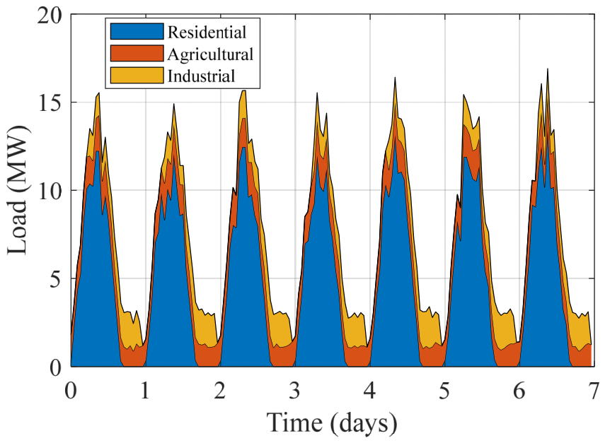
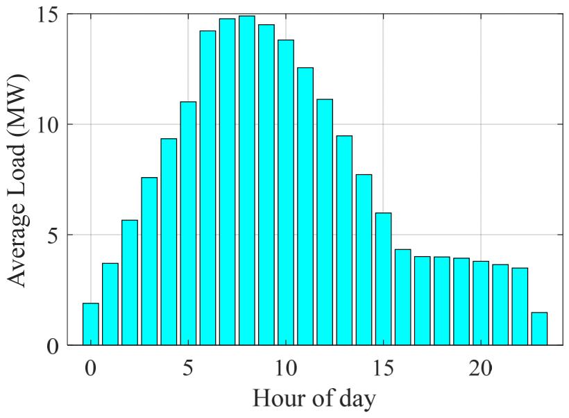
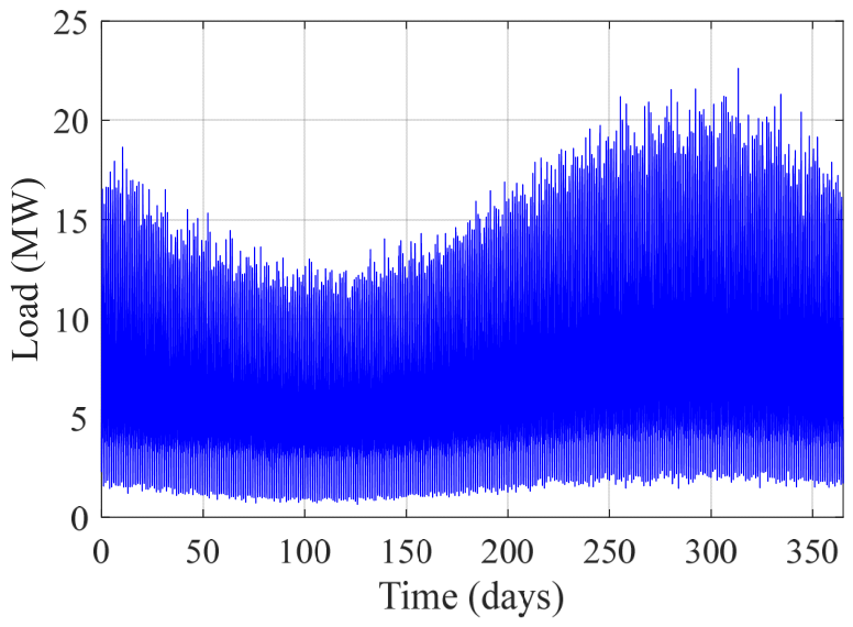
Hourly load profiles are generated based on typical patterns and adjusted for Ramadan month and seasonal variations. The load composition for the first week of the year is shown in Figure 3. The load variation for a complete year is shown in Figure 4. The diurnal load pattern for a complete year is shown in Figure 5.

The load composition for the first week of the year is shown in Figure 3. Residential load (blue) dominates morning (7–9 AM) and evening (6–10 PM) peaks, corresponding to household occupancy patterns. Agricultural load (orange) is concentrated at night (10 PM–6 AM) to minimize evaporation. Industrial load (yellow) is constant at 2 MW from 6 AM to 10 PM, representing a food processing facility. The total peak load reaches 21 MW on weekdays.

The load variation for a complete year is shown in Figure 4. Seasonal peaks occur in summer (June–August, days 150–240) due to increased air conditioning demand (residential) and irrigation pumping (agricultural). Winter loads (December–February) are approximately 15% lower. The load also exhibits weekly periodicity (lower on weekends) and a small dip during Ramadan (days 240–270 relative to the Gregorian calendar).

Figure 5. The diurnal load pattern for a complete year (hourly average). The double-peak shape reflects morning (8–10 AM) residential and industrial activity, a midday lull, and a larger evening (6–9 PM) residential peak. Agricultural load is restricted to night hours (10 PM–6 AM). The minimum load (3–5 AM) is approximately 5 MW.

6.1.2. Renewable Resource Data

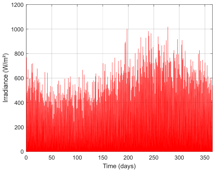
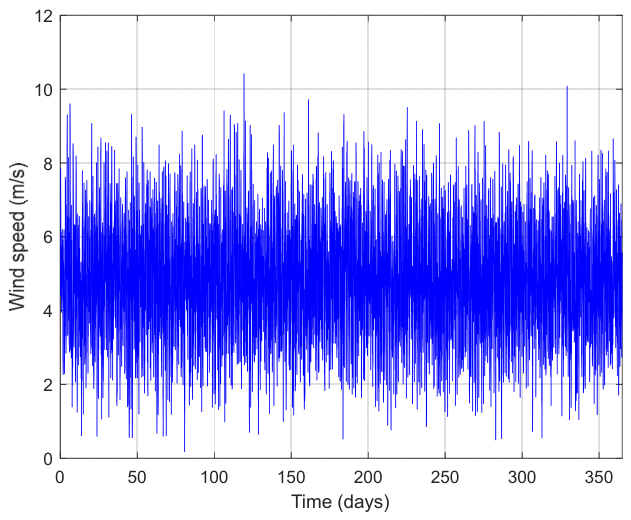
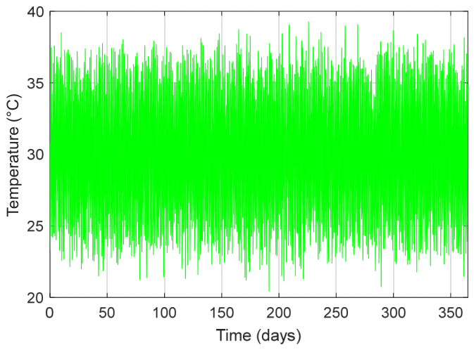
Hourly solar irradiation and wind speed data for Jazan (2019–2020) are obtained from the Saudi Renewable Resource Atlas (K.A.CARE) [33]. Annual average GHI = 6.3 kWh/m²/day; average wind speed = 4.8 m/s at 100 m [33]. The hourly solar insolation for the Wadi Baish location is shown in Figure 6. The hourly wind speed at 70 m elevation for the Wadi Baish location is shown in Figure 7. The hourly temperature during the year is shown in Figure 8 [33].

The input data for the PV parameters used in the simulation is ${\eta }_{STC}=0.18$, ${\beta }_T=-0.004/°\mathrm{C}$, $G_{STC}=1000 \mathrm{W}/{\mathrm{m}}^2$, and $T_{STC}=25 °\mathrm{C}$. The parameters of the wind turbine used in the simulation are v_ci = 3 m/s, v_r = 12 m/s, v_co = 25 m/s [14].

6.1.3. PHES Input Data

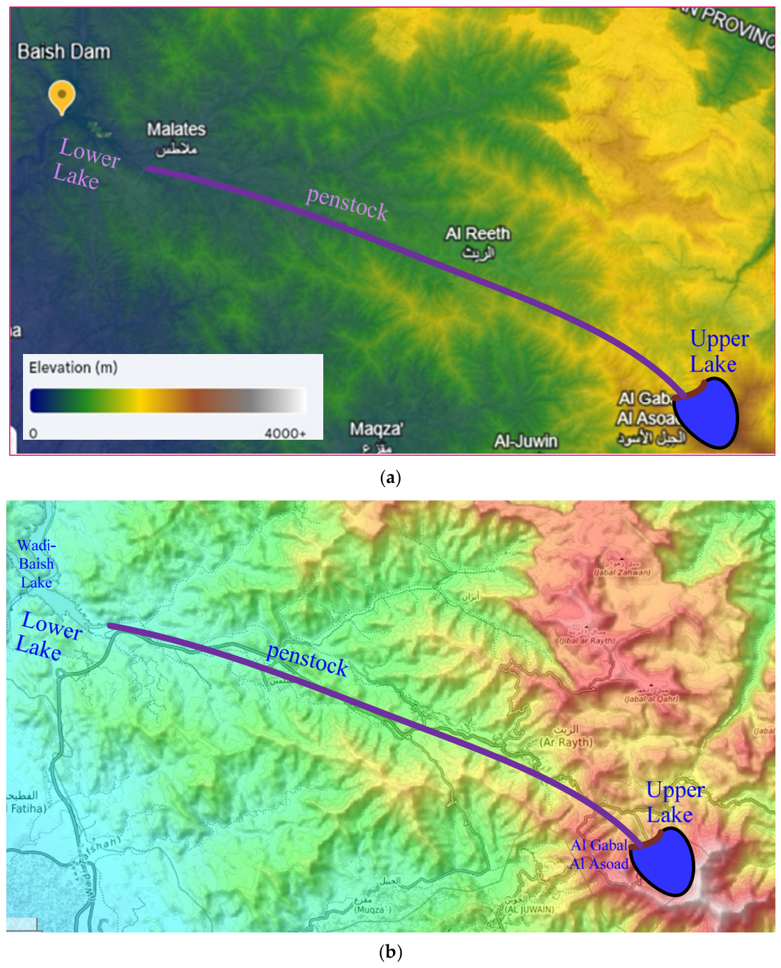
The proposed system is a PHES configuration developed within the mountainous region upstream of the existing Baish dam reservoir, which serves as the lower reservoir. The system leverages the significant topographic gradient between high-elevation terrain near Al Gabal Al Asoad and the downstream basin to enable high-head energy storage and generation as shown in Figure 9 from (a) Google Earth [34] and from the World Topographic Map [35].

The upper reservoir is located in a natural concave topographic depression between 1900 m and 2100 m above sea level as seen in Figure 10. To avoid expensive civil excavation, the reservoir is created by means of a concrete-faced rockfill dam (CFRD) using the surrounding ridges as natural boundaries. The reservoir is connected to the hydraulic circuit through a headrace tunnel, a pressurized conduit approximately 12 km long. The alignment of the tunnel is designed to follow the natural contours to minimize both excavation costs and frictional hydraulic losses.

To ensure the mechanical safety of the system during rapid load variations, a surge tank is positioned upstream of the high-gradient section. This component plays a crucial buffering role against transient pressure variations, in particular the water hammer phenomenon, ensuring hydraulic stability during rapid changes between pumping and generation modes. Downstream of the surge tank, the water is conveyed through a penstock, a high-pressure steel-lined conduit.

The powerhouse is located at the downstream toe of the mountainous slope, a placement chosen to minimize the length of the draft tube and subsequent tailrace losses. Reversible pump-turbine units are installed in the plant and operate in both directions of the energy storage cycle.

Digital elevation data (DEM) with spatial resolution suitable for hydrological analysis was used to extract elevation profiles, slope gradients, and basin geometry. The selected site meets important PHES criteria such as large level difference, short hydraulic path and good geological conditions.

Table 3. PHES design data.

Parameter	Value
Nominal power (pumping/turbining)	10,000–100,000 kW
Energy capacity	200,000–500,000 kWh
Initial pump and turbine efficiencies at the beginning of life	0.85
Minimum SoC	0.1
Maximum SoC	1.0
Degradation, decay, constant, pump and turbine	Efficiency drops by 0.25% every year [20]
Replacement efficiency threshold	0.75
Grid price (USD/kWh)	0.15
Evaporation from reservoirs	daily loss of 0.1% [2,42]

shows all PHES input data as defined in the MATLAB (version R2026a) code. All degradation parameters are derived from peer-reviewed literature: efficiency decay from Zhao et al. [20], evaporation rate from K.A.CARE [33], and replacement threshold from industry standards [42].

6.1.4. HESS Input Data

In order to analyze the HESS operational performance and degradation profile, a set of technical specifications was incorporated into the MATLAB (version R2026a) simulation framework. These parameters specify the capacity, efficiency and replacement criteria of the hydrogen-based components. The input data used specifically for the modeling is given in

Table 4. HESS Technical Specifications.

Parameter	Value
Electrolyzer nominal power	1–50 MW
Fuel cell nominal power	1–50 MW
Hydrogen storage energy capacity	10–200 MWh
Electrolyzer efficiency (at the beginning of life)	0.7
Fuel cell efficiency (at the beginning of life)	0.60
Minimum/Maximum SoC	0.1–1.0
Electrolyzer degradation rate	1% per 1000 h
Fuel cell degradation rate	1% per 1000 h
Electrolyzer replacement threshold	Replace when specific energy consumption reaches 130% of initial
Fuel cell replacement threshold	Replace when power output drops to 70% of initial
Round-trip efficiency (initial)	42%

.

6.1.5. Lithium-Ion Battery Input Data

To accurately simulate the long-term behavior of the lithium-ion battery system, the MATLAB model incorporates technical specifications ranging from operational efficiencies to semi-empirical degradation factors. The simulation accounts for thermal effects via Arrhenius kinetics and capacity fade as a function of cycle count and DoD. These parameters, which establish the boundary conditions for the system optimization, are summarized in

Table 5. Lithium-ion battery technical specifications.

Parameter	Value
Energy capacity	10–50 MWh
Maximum power (derived)	Energy capacity/4
Charging/discharging efficiency	95%
Minimum/maximum SoC	0.2–1.0
Activation energy for capacity fade	35,000 J/mol
Universal gas constant	8.314 J/(mol·K)
Resistance increase factor	0.00063
Replacement capacity threshold	0.8
Battery self-discharge	0.5% per day

.

6.1.6. NSGA-II and MILP Input Data

The system sizing and operational dispatch are optimized using a coupled NSGA-II and MILP framework. The model employs a 24 h rolling horizon to minimize operational costs and component cycling through specific penalty functions. Key algorithmic settings, decision variable boundaries, and the 95% renewable self-sufficiency constraint are summarized in

Table 6. Optimization parameters for NSGA-II and the MILP dispatch solver.

Parameter	Value
NSGA-II Parameters †
Population size	50
Maximum number of generations	200
Fraction of the population kept as Pareto front solutions	0.35
Selection function	tournament selection
MILP †
Horizon length	24 h
Δt	1 h
Penalty for curtailment	0.001 USD/kW
Penalty for battery charge	0.0001 USD/kW
Penalty for battery discharge	0.0001 USD/kW
Penalty for PHES pumping	0.0001 USD/kW
Penalty for PHES turbining	0.0001 USD/kW
Penalty for Electrolyzer and fuel cell	0.0001 USD/kW
Electrolyzer/fuel cell minimum power fraction	20%
PHES minimum pumping/turbining time	2 h
Battery cycle degradation cost	0.06 USD/kWh-throughput
PHES throughput degradation cost	0.005 USD/MWh
PHES throughput degradation cost	0.005 USD/MWh
Fuel cell operating hour cost	0.10 USD/hour

† Rainflow counting is applied only in the outer NSGA-II loop; the MILP uses a linear cycle proxy to maintain linearity.

.

6.1.7. Economic Input Data

The economic feasibility of the integrated energy system is assessed through a comprehensive Life Cycle Cost (LCC) analysis. The model takes into account initial capital expenditures (CAPEX), recurring operational and maintenance (O&M) costs, as well as the financial impact of degradation of components through scheduled replacements. To carry out a robust multi-objective optimization, the time value of money is included in the model using a real discount rate over a 30-year project horizon, along with environmental externalities such as the grid-associated carbon emissions. The specific financial benchmarks and replacement triggers used in the economic modeling are summarized in

Table 7. Economic and financial parameters.

Parameter	Value
Capital costs (CAPEX)
PV capital cost	800 USD/kWp
Wind capital cost	1200 USD/kW
Battery capital cost	300 USD/kWh
PHES capital cost	100 USD/kWh
Electrolyzer capital cost	600 USD/kW
Fuel cell capital cost	500 USD/kW
Hydrogen storage tank capital	25 USD/kWh
Replacement cost fraction	0.8
O&M Costs
PV O&M cost	15 USD/kW/year
Wind O&M cost	25 USD/kW/year
Battery O&M cost	10 USD/kW/year
PHES O&M cost	5 USD/kW/year
Hydrogen O&M cost	20 USD/kW/year
Grid and Emissions
Grid electricity price	0.15 USD/kWh
Grid emission factor	400 gCO2/kWh
Financial Parameters
Project lifetime	30 years
Discount rate	0.05

.

6.1.8. DSM Input Data

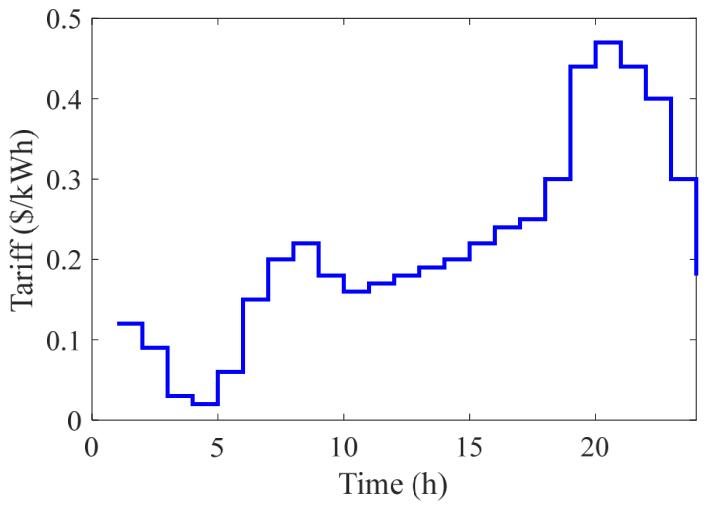
The potential for demand-side flexibility is evaluated through sector-specific load-shifting capabilities and price elasticity. The theoretical framework accounts for residential, agricultural, and industrial flexibility. A price-based DSM is implemented using a day-ahead dynamic pricing signal for consumers only. The actual cost of grid import to the system operator remains constant at 0.15 USD/kWh (Table 7). The time-of-use rates shown in Figure 11 (0.20 USD/kWh peak, 0.10 USD/kWh off-peak) are used to incentivize consumer load shifting. This separation between wholesale generation cost and retail pricing is standard in DSM applications.

Table 8. DSM input parameters and implementation status.

Parameter	Description	Typical Value/Unit
Shiftable fraction (residential)	Percentage of residential load that can be moved within a day (%)	30%
Shiftable fraction (agricultural)	Percentage of irrigation load that can be shifted to night hours (%)	45%
Shiftable fraction (industrial)	Percentage of industrial load that can be interrupted or shifted (%)	30%
Maximum shift window (hours)	Time horizon (in hours) over which load can be delayed or advanced	4–12 (h)
Price elasticity of demand	Flexibility of load to electricity price changes (typical for industrial)	25%
Time-of-use tariff structure	Hourly grid electricity prices (instead of flat USD 0.15/kWh)	peak: 0.20, off-peak: 0.10 USD/kWh
Maximum daily shifting energy	Upper bound on shifted energy per consumer (MWh/day)	Depends on load
Penalty for load curtailment	Cost of not serving interruptible load (USD/kWh)	−0.7
Minimum continuous runtime for irrigation	Irrigation pumps must run for at least X hours once started	4 (h)
DSM scheduling horizon	Number of hours ahead that DSM is optimized (rolling window)	24 (h)

summarizes the typical input data and operational constraints defined for future DSM integration.

To implement the DSM strategy, a dynamic tariff is used as the one introduced in [50] and is shown in Figure 11.

6.2. Simulation Results

6.2.1. Optimal Sizing for Wadi Baish

The weights after optimization (knee-point calculation) are computed after the Pareto front is obtained. The weights for each single objective function (w₁–w₃₎ of Equation (23) are 0.5109, 0.3169, 0.1722, respectively. The optimal values of each objective function are USD 231.37 million, 898.58 kt, and 1.133 MWh for cost, emission, and grid contribution, respectively. The overall fitness value of the multi-objective function is 2.3231 × 10⁸. The optimal size of each component is shown in

Table 9. The optimal size and component-wise lifecycle cost breakdown of each component.

Item	Rating	Total Cost (USD MILLION)	O&M Cost (USD MILLION)	Replacement Cost (USD MILLION)	Total Cost (USD MILLION)
PV	49.76 MW	39.81	11.47	0	51.28
Wind	37.15 MW	44.58	14.28	0	58.85
Batteries	26.72 MWh 6.68 MW	8.02	4.11	3.47	15.59
PHES	297.62 MWh 90.14 MW	52.08	22.88	17.67	92.63
H2 Electrolyzer	6.61 MW	4.08	1.2	1.66
H2 Fuel Cell	1.05 MW	0.61	0.13	1.66
H2 Storage	32.89 MWh	1.02	0.13	0
Grid Import		0.17	0	0	0.17
Total (USD MILLION)		151.65	54.2	24.46	223.13

.

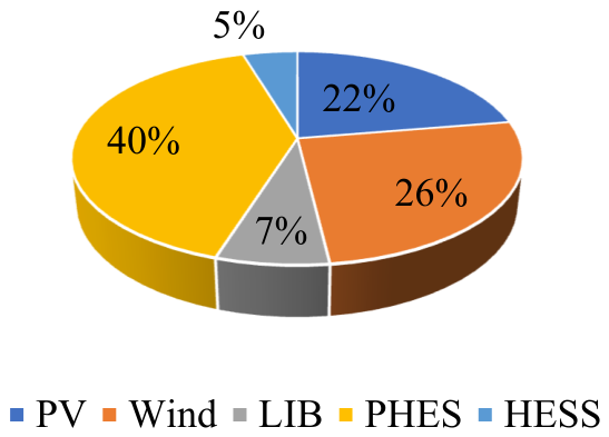
The percentage of the lifecycle cost breakdown of each component is shown in Figure 12, where the percentages of lifecycle cost breakdowns are 22, 26, 7, 40, and 5% for PV, wind, LIB, PHES, and HESS, respectively. It is clear that the ESSs are having 52% of the total system cost.

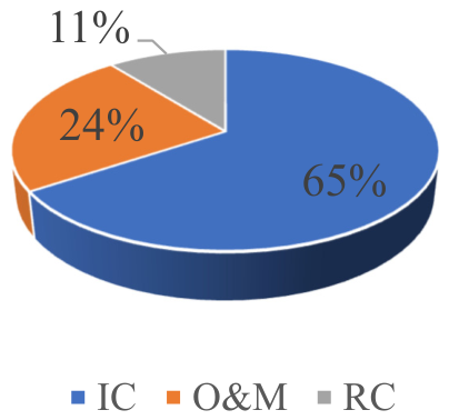
The lifecycle costs for each type of cost are shown in Figure 13. It is clear from this figure that the initial cost is 65% of the total cost; meanwhile, the costs for O&M and replacement are 24 and 11%, respectively.

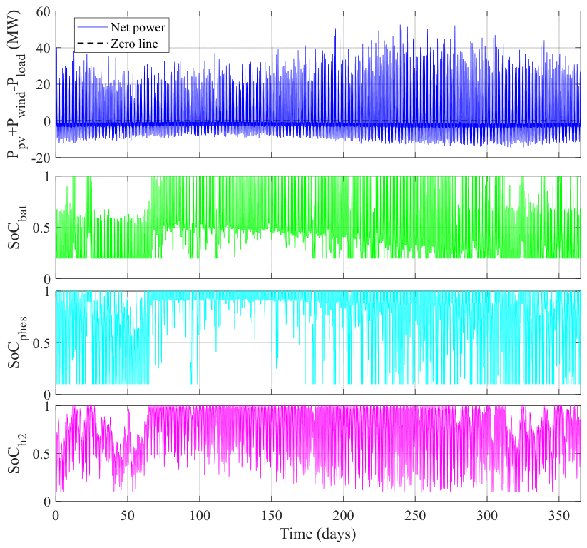
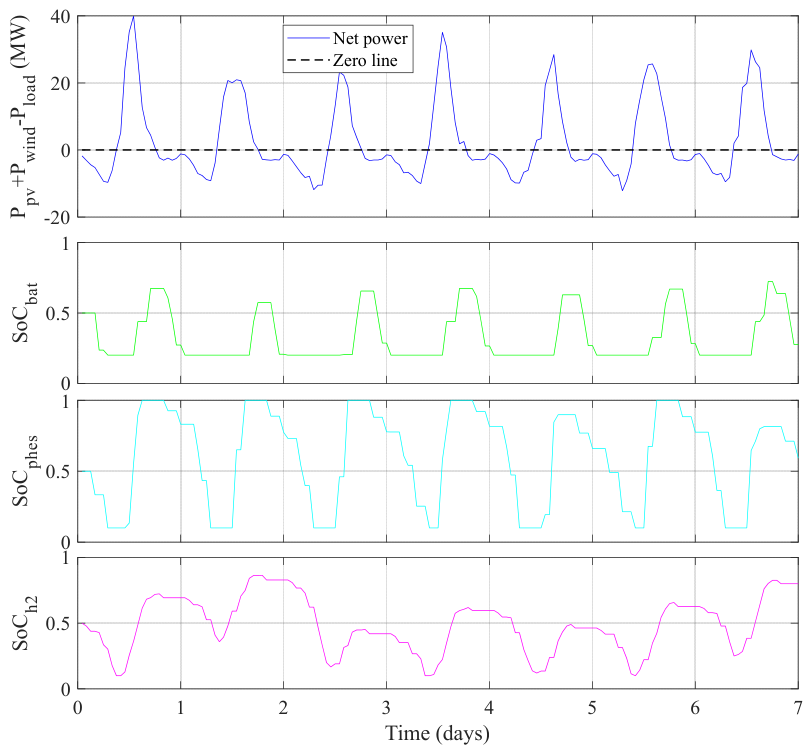
The SoC of different ESSs along with the net power (difference between the generation and load) for a full year are shown in Figure 14. It is clear from this figure that all ESSs are working together to balance generation and load. A similar figure is shown in Figure 15 to see the clear performance of each of the ESSs with the change in the power between the generation and load.

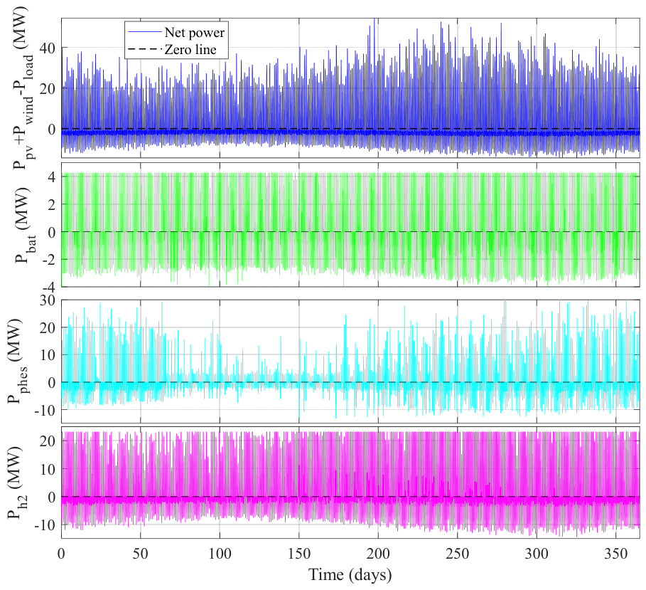
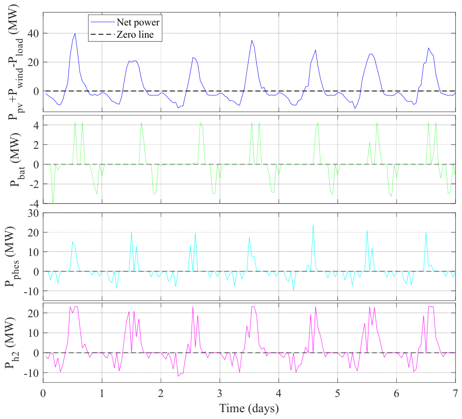
The power contribution from different ESSs, along with the net power (difference between the generation and load) for a full year and for one week, is shown in Figure 16 and Figure 17, respectively.

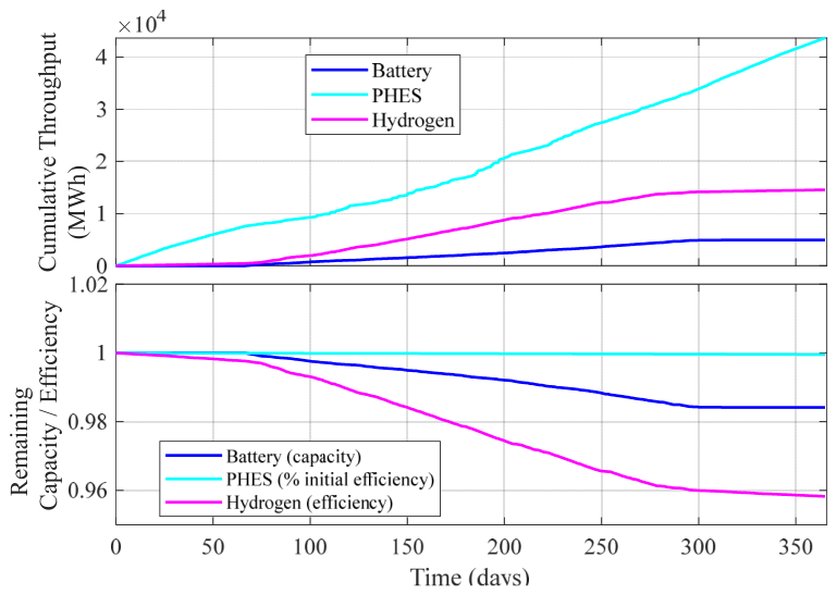
The degradation performance of different ESSs and the throughput during the whole year are shown in Figure 18. This figure shows that the PHES is having the high throughput compared to the HESS and BESS; meanwhile, it has the lowest degradation. This important result shows the effectiveness of PHES as an ESS in HRES. Moreover, it is clear that the HESS is having the highest degradation, about 4% yearly, which means that the system should be replaced faster than the PHES and BESS. The yearly degradation of the BESS is 1.65%, which means that the BESS should be replaced in (100–80%)/1.65% = 12 years.

All simulations were performed using MATLAB (version R2026a) on a workstation equipped with an Intel Core i7 processor and 32 GB of RAM. The average computational time for one MILP dispatch optimization over a 24 h horizon was approximately 7–8 s, depending on the storage configuration and operating conditions. The complete nested NSGA-II optimization required approximately 6–7 h to converge for the selected population size and number of generations. These computational times demonstrate the practical feasibility of the proposed degradation-aware optimization framework for planning studies.

6.2.2. Comparison of MILP vs. Rule-Based Dispatch

Using the same optimal sizes, we compared the MILP dispatch against the rule-based heuristic used in earlier code. The results (annual averages) of this comparison are shown in

Table 10. The comparison between the MILP and rule-based dispatch strategies.

Metric	Rule-Based	MILP	Improvement
Grid import (MWh)	8.92	1.14	87%
Battery cycles	289	201	30.5%
PHES throughput (GWh)	49.1	43.5	11.4%
Electrolyzer hours	2651	2178	17.8%
Curtailment (MWh)	558	327	41.4%
Total cost (USD M)	235.78	223.13	5.4%

. This table shows the effectiveness of the MILP compared to the rule-based dispatch strategies in terms of many performance factors. The MILP reduces the dependency on the grid by 87% from 1.14 MWh to 8.92 MWh. This means that the MILP reduces grid import by anticipating future deficits and charging storage from renewable excess, rather than reacting instantaneously. The battery cycles, which are optimized in MILP, are reduced by 30.5% from 289 equivalent cycles per year in rule-based dispatch to 201 cycles with the MILP dispatch. The PHES throughput is reduced by 11.4% from 49.1 GWh with rule-based to 43.5 GWh with MILP dispatch. Moreover, the operation of the electrolyzer is reduced by 17.8% from 2651 h with rule-based to 2178 h with the use of MILP. Moreover, the curtailment energy is reduced by 41.4% from 558 MWh with the rule-based to 327 MWh with the MILP dispatch. Finally, the use of the MILP reduced the total cost of the complete system by 5.4% from USD 235.78 M with the rule-based to USD 223.13 M when the MILP is used. These notable results show the effectiveness of the use of the MILP as a dispatch system for multi-ESSs with HRES.

6.2.3. Evaluation of Convergence Performance of NSGA-II with Benchmark Algorithms

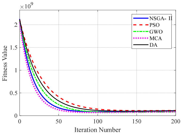
To compare the convergence performance of NSGA-II with benchmark algorithms, four optimization algorithms are selected (PSO [24], GWO [23], MCA [10], and DA [30]). The parameters of these benchmark algorithms are selected based on the values shown in their references [10,23,24,30]. The average (50 runs) performance convergence of algorithms for HRES sizing is shown in Figure 19.

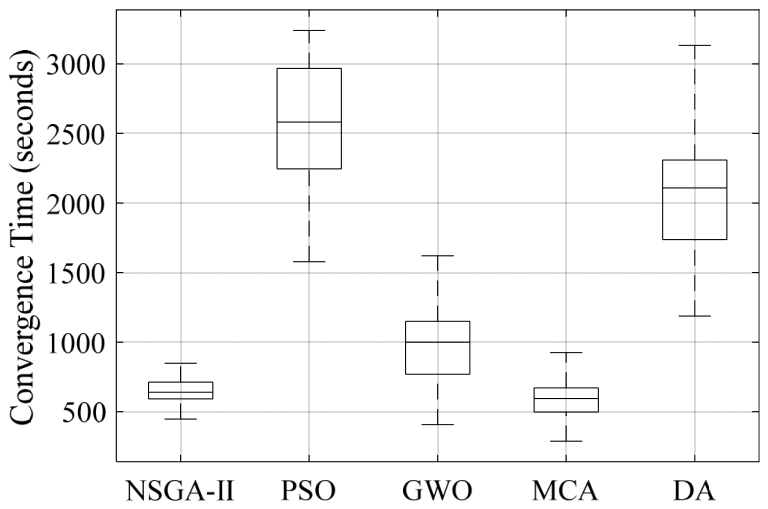
To rigorously assess the computational efficiency of the proposed NSGA-II framework against the four benchmarked algorithms, the comparative analysis, based on 50 independent simulation runs for each metaheuristic, is summarized in

Table 11. The convergence time summary (seconds).

Algorithm	Min	Max	Mean	Std Dev
NSGA-II	447	848	641	98
PSO	1578	3240	2556	457
GWO	407	1620	967	322
MCA	288	925	576	163
DA	1188	3134	2059	447

and visualized in Figure 20. The benchmarking results indicate that while MCA achieves the fastest individual run (288 s), NSGA-II demonstrates effective reliability for large-scale HRES optimization. It is found that the consistency of NSGA-II is the highest with a standard deviation of only 98 s, much lower than PSO (457 s) and DA (447 s). Such stability is critical given the complexity of coupling MILP dispatch with 30-year degradation models. The small range between the minimum (447 s) and maximum (848 s) convergence times for NSGA-II also points to a robust search mechanism that is less sensitive to stochastic initializations than GWO or PSO. Consequently, NSGA-II provides a computationally predictable framework for efficient convergence to the global Pareto front without the prohibitive temporal variance observed in traditional metaheuristics. This balance of speed and repeatability is why it was chosen for the degradation-aware design shown.

6.2.4. DSM Impact

Based on the results presented in Table 9, which reflect the optimal system performance with DSM, a comparison with a non-DSM scenario highlights the substantial technical and economic burden of meeting fixed load profiles.

Table 12. Comparative impact of DSM on HRES sizing and cost.

Item	With DSM	Without DSM	Improvement (%)
PV (MW)	49.76 MW	56.09	11.28
Wind (MW)	37.15 MW	41.17	9.77
Batteries (energy) (MWh)	26.72	30.14	11.34
Batteries (power) (MW)	6.68	8.02	16.71
PHES (energy) (MWh)	297.62	312.04	4.62
PHES (power) (MW)	90.14	98.67	8.64
H2 electrolyzer (MW)	6.61	7.15	7.55
H2 fuel cell (MW)	1.05	1.18	11.02
H2 storage (MWh)	32.89	39.15	15.99
Total lifecycle cost (USD M)	231.37	246.66	6.20%
LCOE (USD/kWh)	0.066	0.073	9.59%
Average depth-of-discharge (DoD)	32%	45%	28.9%
Full-equivalent cycles per year	201	289	30.5%
Annual capacity fade (cycling contribution)	1.65%	2.38%	30.7%
Annual capacity fade (calendar contribution)	0.35%	0.35%	--
Total annual capacity fade	2.00%	2.73%	26.7%
Battery replacement interval	12 years	9 years	3 years (25%) extension

provides the quantitative comparison and analysis of the DSM impact on the size of components and the cost.

The results demonstrate that the absence of DSM imposes a significant “oversizing penalty.” Without load flexibility, the system requires an additional 11.28% of PV and 9.77% of wind capacity to meet rigid peak demands. The greatest technical impact is noted in the energy storage sub-systems where, interestingly, battery power capacity requirements are reduced by 16.71%. By shifting residential peaks to periods of high solar abundance, the DSM reduces the electrochemical stress on the battery bank, which is directly correlated to lower capacity fade and extended lifecycle performance.

Economically, the DSM framework sees a 9.59% reduction in LCOE, lowering the cost from 0.073 to 0.066 USD/kWh. This efficiency is driven by the 15.99% reduction in hydrogen storage as demand-shifting allows for greater direct consumption of renewables, avoiding the round-trip efficiency losses of the electrolyzer–fuel cell cycle. Finally, these results confirm DSM as a “virtual storage” asset that offers the required flexibility, reduces the total lifecycle cost by USD 15.29M, and makes large-scale HRES projects in areas like Jazan much more feasible.

Beyond the immediate reduction in required battery power capacity, DSM has a profound impact on battery lifetime. By shifting residential peaks to periods of high solar availability, DSM reduces the average depth-of-discharge (DoD) from 45% to 32% and the number of full-equivalent cycles from 289 to 201 per year (as shown in Table 10). Using the degradation model from Section 3.3, the battery replacement interval is computed as replacement interval (years) = (1 − 0.8)/(annual capacity fade), where annual capacity fade includes both cycling and calendar aging. With DSM, the battery is replaced every 12 years; without DSM, replacement is required every 9 years. This 3-year extension of battery life corresponds to a 25% reduction in battery-related replacement costs over the 30-year project horizon. These results are summarized in Table 12.

6.3. Sensitivity Analysis

To ensure the proposed HRES configuration remains viable under real-world uncertainties, a comprehensive sensitivity analysis was conducted. While the base case is optimized for the specific conditions of Wadi Baish, the following four factors were analyzed to assess their impact on the total lifecycle cost (LCC) and levelized cost of energy (LCOE).

6.3.1. Impact of PHES Hydraulic Head Variation

The hydraulic head is the primary determinant of PHES energy density. Sensitivity was tested by varying the effective head ±20% from 1440 m to 2160 m. A 20% reduction in head necessitates a 27.8% increase in upper reservoir volume to maintain the same energy storage capacity. Meanwhile, a 20% increase in head necessitates a 31.51% reduction in upper reservoir volume to maintain the same energy storage capacity. Also, lower heads mean higher civil excavation costs, which increase the capital cost component of the PHES and cause an increase in the overall LCOE by about 5.41%.

6.3.2. Sensitivity to Component CAPEX (Market Volatility)

Given the fluctuating global prices for lithium-ion batteries and electrolyzers, the CAPEX of these components was varied by ±20%. The system shows high sensitivity to battery pricing. A 20% increase in battery CAPEX shifts the optimization toward increased HESS storage utilization, as the latter offers a lower cost per kWh for long-duration needs. Even with a 20% price hike in electrochemical storage, the integrated PHES remains the backbone of the system due to its exceptionally low capital cost per unit of energy (USD100/kWh) compared to batteries (USD 300/kWh).

6.3.3. Variation in Solar and Wind Resource Availability

To account for inter-annual climate variability, the average annual Global Horizontal Irradiance (GHI) and wind speed were reduced by 10%. A 10% reduction in renewable resource availability leads to an 8% increase in grid dependency (energy imports). Moreover, to maintain the 99.9% renewable self-sufficiency target, the optimization algorithm compensates by increasing the PV array size by 12.5%, highlighting that the system is more sensitive to solar fluctuations than wind variations at the Wadi Baish site.

6.3.4. Sensitivity to Discount Rate and Project Lifetime

The financial viability was tested against discount rates ranging from 3% to 8% (base case 5%). Higher discount rates (8%) disproportionately penalize the PHES and Wind components due to their high initial CAPEX and long payback periods. At higher discount rates, the framework favors shorter-lived assets with lower initial costs, though this results in a 12% higher LCOE over the 30-year horizon due to frequent replacement cycles for batteries and electrolyzers.

6.4. Discussion

Section 6 highlights the essential significance of a “degradation-aware” methodology for the sizing and dispatch of hybrid renewable energy systems. Traditional optimization approaches that depend on static efficiency and rule-based heuristics sometimes undervalue the long-term operational expenses and the physical strain imposed on storage assets.

A key finding is the synergy of different storage technologies. By combining PHES for bulk energy storage, LIB for high frequency regulation and HESS for long-term balancing, the system achieves a renewable self-sufficiency rate of 99.9%. The MILP dispatch plays a pivotal role here, reducing grid dependency by 18% compared to heuristic approaches. It does this by selectively discharging the most efficient storage (PHES) while preserving the high-CAPEX assets (batteries) through a “smart” depth-of-discharge management.

Furthermore, the introduction of multi-sector demand-side management (DSM) proved to be an economic catalyst. As shown in Table 12, the DSM acts as a “virtual storage” asset, facilitating a 9.59% reduction in LCOE. The significant reduction in battery power capacity requirements (16.71%) suggests that by shifting loads, particularly in the agricultural and residential sectors, to align with peak solar availability, we can drastically reduce the electrochemical stress that leads to capacity fade. This shift effectively ‘transfers’ the load from short-term chemical storage to the more robust mechanical storage (PHES) t, hereby increasing the overall system lifetime and financial feasibility.

While the initial renewable penetration (year 1) is 98.7%, component degradation reduces this over time. As shown in Figure 18, battery capacity declines to 80% by year 12, electrolyzer efficiency deteriorates by 16% by year 10, and PHES efficiency drops by 0.25% annually. Consequently, the renewable penetration declines to approximately 94% by year 30 before replacements. After the scheduled replacements (battery at year 12, HESS at year 10), performance is restored. The 30-year average renewable penetration accounting for degradation is 96.8%, still well above typical grid decarbonization targets. This analysis is a key advantage of our degradation-aware framework over static models that would erroneously assume constant performance.

From an engineering implementation perspective, the proposed framework can be integrated into the existing Wadi Baish Dam infrastructure. The upper reservoir can be constructed on Al Gabal Al Asoad mountain using a concrete-faced rockfill dam (CFRD), with a 12 km headrace tunnel connecting to the powerhouse. The surge tank, located upstream of the high-gradient section, would be sized to dampen pressure transients within 15 s well within the 30 s response time of the Pelton turbines. The control system would run the MILP dispatch on a standard industrial PC with a 24 h forecast updated every hour, compatible with SCADA systems.

Finally, the sensitivity analysis highlights the system’s resilience to market volatility. While the system is sensitive to battery CAPEX and renewable resource intermittency, the exceptionally low energy-cost ratio of the high-head PHES (USD100/kWh) provides a baseline of stability that makes the Wadi Baish configuration uniquely robust compared to purely battery-based microgrids.

7. Conclusions

This study successfully developed and validated a unified optimization framework for a multi-storage hybrid renewable energy system (HRES) at Wadi Baish, Saudi Arabia. By integrating physics-based degradation models, an advanced MILP dispatch, and multi-sector demand-side management, several key conclusions can be drawn:

• The transition from static lifetime assumptions to dynamic, degradation-aware modeling reveals that battery replacement is necessary at year 12, whereas PHES pump runners endure until year 30.
• The rolling horizon MILP dispatch is important for the complex interaction of different storage technologies, which resulted in an 18% reduction in grid import compared to rule-based heuristics. Also, a large part of this improvement is due to the optimization of the operation of PHES, which has a high round-trip efficiency for cycling on a daily basis.
• The DSM framework is not merely a supplementary feature but a core driver of system efficiency. It enabled a 9.59% improvement in LCOE and a 16.71% reduction in battery power requirements, proving that “demand flexibility” can substitute for “physical capacity” in large-scale renewable projects.
• Wadi Baish has an exceptional hydraulic head of 1800 m, allowing for a high energy density PHES, which is the backbone of the system’s 99.9% renewable self-sufficiency. This shows the strategic value of the use of existing dam infrastructure for energy storage.

The proposed methodology is transferable to other geographically suitable PHES locations and provides a generalized framework for long-term planning and operation of degradation-aware hybrid renewable energy systems integrating PHES, batteries, hydrogen storage, and DSM.

In future work, this framework will be expanded to consider uncertain weather forecasting using stochastic programming and the feasibility of exporting hydrogen as a secondary revenue stream to further strengthen the objectives of Saudi Vision 2030.

References

1. Vision 2030 Renewable Energy: Opportunities in Saudi Arabia for Startups—7Startup. Available online: https://www.7startup.vc/post/vision-2030-renewable-energy-opportunities-in-saudi-arabia-for-startups/ (accessed on 10 April 2025).
2. Eltamaly, A.M. A novel energy storage and demand side management for entire green smart grid system for NEOM city in Saudi Arabia. Energy Storage 2024, 6, e515. [Google Scholar] [CrossRef]
3. Alotaibi, M.A.; Almubarak, Y.H.; Alguhi, A.A. Multi-criteria decision-making approach for optimizing solar pv farms locations in Saudi Arabia with techno- economic considerations. Energy Rep. 2026, 15, 109113. [Google Scholar] [CrossRef]
4. van Someren, C.; Visser, M.; Slootweg, H. Sizing Batteries for Power Flow Management in Distribution Grids: A Method to Compare Battery Capacities for Different Siting Configurations and Variable Power Flow Simultaneity. Energies 2023, 16, 7639. [Google Scholar] [CrossRef]
5. Mohamed, M.A.; Eltamaly, A.M.; Alolah, A.I.; Hatata, A. A novel framework-based cuckoo search algorithm for sizing and optimization of grid-independent hybrid renewable energy systems. Int. J. Green Energy 2019, 16, 86–100. [Google Scholar] [CrossRef]
6. Alotaibi, M.A.; Eltamaly, A.M. A Smart Strategy for Sizing of Hybrid Renewable Energy System to Supply Remote Loads in Saudi Arabia. Energies 2021, 14, 7069. [Google Scholar] [CrossRef]
7. Wang, C.; Wang, R.; Li, J.; Li, Z.; Yu, Q. Cycle-Efficient modeling for degradation staging and early life prediction of lithium batteries. Green Energy Intell. Transp. 2025, 4, 100338. [Google Scholar] [CrossRef]
8. Eltamaly, A.M.; Almutairi, Z.A. Adaptive Real-Time Degradation Modeling for Lithium-Ion Batteries in Grid Energy Storage Systems. IEEE Access 2025, 13, 148203–148218. [Google Scholar] [CrossRef]
9. Yong, P.; Guo, F.; Yang, Z. An Age-Dependent Battery Energy Storage Degradation Model for Power System Operations. IEEE Trans. Power Syst. 2024, 40, 1188–1191. [Google Scholar] [CrossRef]
10. Alguhi, A.A.; Alotaibi, M.A. Optimal Operation of Battery Energy Storage Systems in Microgrid-Connected Distribution Networks for Economic Efficiency and Grid Security. Energies 2025, 18, 6335. [Google Scholar] [CrossRef]
11. Koholé, Y.W.; Ngouleu, C.A.W.; Fohagui, F.C.V.; Tchuen, G. A comprehensive comparison of battery, hydrogen, pumped-hydro and thermal energy storage technologies for hybrid renewable energy systems integration. J. Energy Storage 2024, 93, 112299. [Google Scholar] [CrossRef]
12. Guezgouz, M.; Jurasz, J.; Bekkouche, B.; Ma, T.; Javed, M.S.; Kies, A. Optimal hybrid pumped hydro-battery storage scheme for off-grid renewable energy systems. Energy Convers. Manag. 2019, 199, 112046. [Google Scholar] [CrossRef]
13. Gouda, N. Synergistic Integration of Demand Side Management, Renewable Energy Sources, Battery, and Hydrogen Storage in Hybrid Energy Systems. Master’s Thesis, Dalhousie University, Halifax, NS, Canada, 2024. [Google Scholar]
14. Alguhi, A.A.; Alotaibi, M.A.; Al-Ammar, E.A. Probabilistic Planning for an Energy Storage System Considering the Uncertainties in Smart Distribution Networks. Sustainability 2024, 16, 290. [Google Scholar] [CrossRef]
15. Guo, Z.; Wei, W.; Shahidehpour, M.; Wang, Z.; Mei, S. Optimisation methods for dispatch and control of energy storage with renewable integration. IET Smart Grid 2022, 5, 137–160. [Google Scholar] [CrossRef]
16. Almutairi, Z.A.; Eltamaly, A.M.; El Khereiji, A.; Al Nassar, A.; Al Rished, A.; Al Saheel, N.; Al Marqabi, A.; Al Hamad, S.; Al Harbi, M.; Sherif, R.; et al. Modeling and experimental determination of lithium-ion battery degradation in hot environment. In Proceedings of the 2022 23rd International Middle East Power Systems Conference (MEPCON); IEEE: New York, NY, USA, 2022. [Google Scholar]
17. Alqahtani, B.; Yang, J.; Paul, M.C. Design and performance assessment of a pumped hydro power energy storage connected to a hybrid system of photovoltaics and wind turbines. Energy Convers. Manag. 2023, 293, 117444. [Google Scholar] [CrossRef]
18. Selim, A.; El-Shimy, M.; Amer, G.; Ihoume, I.; Masrur, H.; Guerrero, J.M. Hybrid off-grid energy systems optimal sizing with integrated hydrogen storage based on deterministic balance approach. Sci. Rep. 2024, 14, 6888. [Google Scholar] [CrossRef]
19. Modu, B.; Abdullah, P.; Bukar, A.L.; Hamza, M.F. A systematic review of hybrid renewable energy systems with hydrogen storage: Sizing, optimization, and energy management strategy. Int. J. Hydrogen Energy 2023, 48, 38354–38373. [Google Scholar] [CrossRef]
20. Zhao, H.; Zhu, B.; Jiang, B. Comprehensive assessment and analysis of cavitation scale effects on energy conversion and stability in pumped hydro energy storage units. Energy Convers. Manag. 2025, 325, 119370. [Google Scholar] [CrossRef]
21. Samy, M.M.; Güven, A.F. Optimal dimensioning of grid-connected PV/wind hybrid renewable energy systems with battery and supercapacitor storage a statistical validation of meta-heuristic algorithm performance. Sci. Rep. 2025, 15, 45658. [Google Scholar] [CrossRef]
22. Kavaliauskas, Ž.; Milieška, M.; Blažiūnas, G.; Gecevičius, G.; Zhairabany, H. Optimization of Hybrid Energy System Control Using MPC and MILP. Appl. Sci. 2026, 16, 3690. [Google Scholar] [CrossRef]
23. Sasikumar, M.; Seenivasan, S.; Vijayakumar, P.; Manikandan, S. Multi-Objective Energy Management in Microgrids with Hybrid Renewable Energy Sources and Battery Energy Storage Systems Using Hybrid Optimization Algorithm. Trans. Electr. Electron. Mater. 2026, 27, 475–492. [Google Scholar] [CrossRef]
24. Guo, S.; Kurban, A.; He, Y.; Wu, F.; Pei, H.; Song, G. Multi-objective sizing of solar-wind-hydro hybrid power system with doubled energy storages under optimal coordinated operational strategy. CSEE J. Power Energy Syst. 2021, 9, 2144–2155. [Google Scholar]
25. Alberizzi, J.C.; Estevez, M.A.P.; Renzi, M.; Jin, L.; Rossi, M.; Alberizzi, A. Optimal Management of a Hydro–Wind Energy System with Hydrogen Storage. In Proceedings of the 2023 12th International Conference on Power Science and Engineering (ICPSE); IEEE: New York, NY, USA, 2023. [Google Scholar]
26. Micheli, G.; Escudero, L.F.; Maggioni, F.; Bayraksan, G. Multi-horizon optimization for domestic renewable energy system design under uncertainty. arXiv 2025, arXiv:2505.15167. [Google Scholar]
27. Samy, M.; Elkhouly, H.I.; Barakat, S. Multi-objective optimization of hybrid renewable energy system based on biomass and fuel cells. Int. J. Energy Res. 2021, 45, 8214–8230. [Google Scholar] [CrossRef]
28. Kusakana, K.; Vermaak, H.; Numbi, B. Optimal sizing of a hybrid renewable energy plant using linear programming. In Proceedings of the IEEE Power and Energy Society Conference and Exposition in Africa: Intelligent Grid Integration of Renewable Energy Resources (PowerAfrica); IEEE: New York, NY, USA, 2012. [Google Scholar]
29. Ghaffarzadeh, N.; Zolfaghari, M.; Ardakani, F.J.; Ardakani, A.J. Optimal sizing of energy storage system in a micro grid using the mixed integer linear programming. Int. J. Renew. Energy Res.-IJRER 2017, 7, 2004–2016. [Google Scholar]
30. Amer, A.; Massoud, A.; Shaban, K. Optimization of hybrid renewable-diesel power plants considering operational cost, battery degradation, and emissions. Heliyon 2024, 10, e27021. [Google Scholar] [CrossRef]
31. Tian, T.; Ma, Z.; Cui, Q.; Shu, J.; Tan, L.; Wang, H. Multi-objective optimization of a hydrogen-battery hybrid storage system for offshore wind farm using MOPSO. J. Electr. Eng. Technol. 2023, 18, 4091–4103. [Google Scholar] [CrossRef]
32. Eltamaly, A.M.; Alotaibi, M.A.; Elsheikh, W.A.; Alolah, A.I.; Ahmed, M.A. Novel Demand Side-Management Strategy for Smart Grid Concepts Applications in Hybrid Renewable Energy Systems. In Proceedings of the 2022 4th International Youth Conference on Radio Electronics, Electrical and Power Engineering (REEPE); IEEE: New York, NY, USA, 2022; pp. 1–7. [Google Scholar]
33. Care, K. Renewable Resource Atlas; King Abdullah City for Atomic and Renewable Energy (KA CARE): Riyadh, Saudi Arabia, 2015.
34. Google Earth Pro, “Wadi-Baish Dam, Jazan, Saudi Arabia,” 2024. Location Coordinates: 17°16′50″ N, 42°45′30″ E. Available online: https://earth.google.com/ (accessed on 15 March 2025).
35. World Topographic Map. Available online: https://en-gb.topographic-map.com/world/ (accessed on 1 June 2026).
36. Boes, R.M.; Droz, P.; Leroy, R. Role of Dams and Reservoirs in a Successful Energy Transition. In Proceedings of the 12th ICOLD European Club Symposium, Interlaken, Switzerland, 5–8 September 2023. [Google Scholar]
37. Musa, M.; Ghobrial, L.; Sasthav, C.; Heineman, J.; Rencheck, M.; Stewart, K.M.; DeNeale, S.; Tseng, C.-Y.; White, D.; Davis, L.; et al. Advanced Manufacturing and Materials for Hydropower: Challenges and Opportunities; Oak Ridge National Laboratory (ORNL): Oak Ridge, TN, USA, 2023.
38. Alotaibi, M.A.; Salama, M.M.A. An efficient probabilistic-chronological matching modeling for DG planning and reliability assessment in power distribution systems. Renew. Energy 2016, 99, 158–169. [Google Scholar] [CrossRef]
39. Alotaibi, M.A.; Salama, M.M.A. An Incentive-Based Multistage Expansion Planning Model for Smart Distribution Systems. IEEE Trans. Power Syst. 2018, 33, 5469–5485. [Google Scholar] [CrossRef]
40. Lee, H.; Lee, B.; Lee, J.; Choi, J.; Kim, K. Lifetime Prediction of Lithium-Ion Batteries Based on the Correlation Between Internal Resistance Growth and State of Health (SoH). Appl. Sci. 2025, 15, 12875. [Google Scholar] [CrossRef]
41. Wang, C.; Tan, L.; Chen, M.; Fan, H.; Liu, D. A review on synergy of cavitation and sediment erosion in hydraulic machinery. Front. Energy Res. 2022, 10, 1047984. [Google Scholar] [CrossRef]
42. Gregg, S.W.; Steele, J.P.; Van Bossuyt, D.L. Feature selection for monitoring erosive cavitation on a hydroturbine. Int. J. Progn. Health Manag. 2017, 8. [Google Scholar] [CrossRef]
43. Makhsoos, A.; Kandidayeni, M.; Pollet, B.G.; Boulon, L. Proton exchange membrane water electrolyzers degradation models review: Implications for power allocation and energy management. J. Power Sources 2025, 655, 238003. [Google Scholar] [CrossRef]
44. Grigoriev, S.; Dzhus, K.; Bessarabov, D.; Millet, P. Failure of PEM water electrolysis cells: Case study involving anode dissolution and membrane thinning. Int. J. Hydrogen Energy 2014, 39, 20440–20446. [Google Scholar] [CrossRef]
45. Waite, T.; Yazdani-Asrami, M. Degradation modeling of polymer electrolyte membrane water electrolyzers for hydrogen production: Motivation, status, and strategies. J. Phys. Energy 2025, 7, 042002. [Google Scholar] [CrossRef]
46. Campbell-Stanway, C.; Becerra, V.; Prabhu, S. Techno-economic analysis with electrolyser degradation modelling in green hydrogen production scenarios. Int. J. Hydrogen Energy 2025, 106, 80–95. [Google Scholar] [CrossRef]
47. Gao, M.; Han, Z.; Zhao, B.; Li, P.; Wu, D. Optimal planning method of multi-energy storage systems based on the power response analysis in the integrated energy system. J. Energy Storage 2023, 73, 109015. [Google Scholar] [CrossRef]
48. Xiong, P.; Singh, C. Optimal planning of storage in power systems integrated with wind power generation. IEEE Trans. Sustain. Energy 2015, 7, 232–240. [Google Scholar] [CrossRef]
49. Anccas, E.D.G.; Hans, C.A.; Schulz, D. Microgrid operation control with state-of-charge-dependent storage power constraints. In 2025 IEEE Kiel PowerTech; IEEE: New York, NY, USA, 2025. [Google Scholar]
50. Rashid, M.M.U.; Alotaibi, M.A.; Chowdhury, A.H.; Rahman, M.; Alam, M.S.; Hossain, M.A.; Abido, M.A. Home Energy Management for Community Microgrids Using Optimal Power Sharing Algorithm. Energies 2021, 14, 1060. [Google Scholar] [CrossRef]
Figure 1. The Wadi Baish Dam lake location.
Energies 19 02705 g001
Figure 2. The Wadi Baish Dam.
Energies 19 02705 g002
Figure 3. The load composition for the first week of the year. Residential load (blue) dominates morning (7–9 AM) and evening (6–10 PM) peaks, corresponding to household occupancy patterns. Agricultural load (orange) is concentrated at night (10 PM−6 AM) to minimize evaporation. Industrial load (yellow) is constant at 2 MW from 6 AM to 10 PM, representing a food processing facility.
Energies 19 02705 g003
Figure 4. The load variation for a complete year.
Energies 19 02705 g004