Article

The Future Afloat: Potential of Floating Photovoltaics in Arkansas Irrigation Reservoirs

1
Public Policy PhD Program, University of Arkansas, Fayetteville, AR 72701, USA
2
Department of Agricultural Economics and Agribusiness, Division of Agriculture, University of Arkansas System, Fayetteville, AR 72701, USA
3
Department of Biological and Agricultural Engineering, Division of Agriculture, University of Arkansas System, Fayetteville, AR 72701, USA
*
Author to whom correspondence should be addressed.
Energies 2026, 19(11), 2646; https://doi.org/10.3390/en19112646 (registering DOI)
Submission received: 17 April 2026 / Revised: 27 May 2026 / Accepted: 28 May 2026 / Published: 30 May 2026
(This article belongs to the Section A2: Solar Energy and Photovoltaic Systems)

Abstract

Scrutiny over land-based photovoltaic systems (LPV) infringing on agricultural land is increasing with heightened demand for electricity. As a solution, we investigated the electricity generation potential of installing photovoltaic panels on embankments of, and floating in, ~800 irrigation reservoirs covering ~11,300 ha in Arkansas. We compared floating photovoltaic systems (FPV) to LPV using a techno-economic feasibility study that quantified (1) the difference in surface area requirements and installation cost per MW, (2) reduced wave action on embankment erosion with FPV compared to uncovered reservoirs, and (3) evaporation water savings from photovoltaic panel shading. Sensitivity analyses on water area coverage and investor adoption were also performed. Assuming a 5-MW FPV, covering 25% of surface water, and comparing it to a 100-MW LPV, the annual added electricity cost was estimated at 8.99 USD (7.80–10.54) per household (max. +0.7%). With economies of size, larger than 5-MW FPV systems installed on all reservoirs could quadruple photovoltaic capacity compared to 2025 without agricultural land use diversion. Policy options analyzed included (1) subsidizing FPV using a fee on electric bills, (2) continuing federal photovoltaic investment tax credits to lessen installation cost differences between FPV and LPV, (3) encouraging renewable energy portfolio standards, or (4) using funding sources targeted at water savings.

1. Introduction

Investment in photovoltaic (PV) energy generation around the world has increased rapidly over recent years, with 2021 and 2022 representing a 22% increase in global PV energy installations [1]. In 2023, U.S. utility-scale PV energy facilities produced 165 billion kilowatt hours (kWh), or 3.9% of total energy produced in the U.S. [2], which is expected to nearly double by the end of 2025, suggesting continued heavy investment [3].
Arkansas PV capacity ranks 19th in the U.S., with approximately 3.2 gigawatts (GW) in operation as of 2025 [4], with 1.1 GW added in 2024, and an additional 0.4 GW scheduled to become active by the end of 2025 [5]. To provide perspective, 1 MW of PV power during the year has the potential to power up to 180 homes annually (1-MW · 8760 h/yr · 25% capacity factor/12 MWh/per house = 182 homes per year). Approximately 4.4% of energy produced in Arkansas came from PV in 2025 [5]. Countries with a similar share of electricity production from PV include France (5.6%), Thailand (5.3%), Columbia (5.1%), Eswatini (4.9%), and Ireland (4.75%) [6].
While energy capacity relates to the maximum amount of energy that a system can produce under perfect conditions, it does not reflect actual energy output. As such, capacity factors can translate capacity to output over a specified amount of time [7]. A 25% capacity factor is common in the U.S. [8], with more Southern locations with longer daylight hours and sunny climates favored from an efficiency perspective.
The state of Arkansas has passed several laws related to PV energy generation. One of the larger changes came with the passing of Act 278 in 2023, which transitioned the state away from the 1:1 net metering policy that had been in effect. Whereas distributed PV system electricity generators used to get reimbursed for net energy contribution to the grid at rates they paid for electricity they consumed, they are now reimbursed for excess energy at an avoided cost rate which varies by utility but is much lower than the electricity price charged [9]. This is disadvantageous to distributed, smaller-scale energy generators but may not affect larger-scale utility and commercial facilities that typically exceed production capacity limits for net metering eligibility.
Aside from this regulation, PV systems require land. Bolinger and Bolinger (2022) [10] estimated that the most efficient PV systems had 445 kilowatts (kWDC) of capacity per ha of land or 2.25 ha/MW [11] for land-based photovoltaics (LPV). A National Renewable Energy Lab (NREL) study portrayed an average of 3.6 ha/MW [12]. Using these land use efficiencies as a benchmark, the 1.5 GW capacity expansion for 2024–25 in Arkansas required somewhere between 3375 to 5400 ha of land. In contrast, floating PV (FPV) is much less area intensive. Lopes et al.’s (2020) [13] study of FPV installations in Brazil suggested 1.05 ha/MW. Our calculations, detailed in Section 2.1, suggest that available surface areas (water and embankments) on irrigation reservoirs would require approximately 0.75 ha/MW.
With preference for LPV given to cleared, level, and well-drained land, such parcels commonly displace cropland near transmission switching stations but can also occur on marginal land. A solar land lease, typically ranging from 1100 USD to as much as 6200 USD/ha, is more attractive in comparison to cash rent for non-irrigated and irrigated cropland, as well as pasture, which were reported to be 126 USD, 371 USD, and 52 USD/ha, respectively in Arkansas in 2024 [14]. The potential diversion of agricultural land for LPV projects has thus raised concern among Arkansas citizens, as agriculture contributed 14.5% of Arkansas’s value added in 2023 or roughly 24.3 billion USD [15]. With an estimated 15% of PV sites that diverted agricultural land for installation never transitioning back to agriculture [16], fears of sidelining productive agricultural land, currently estimated as high as 1.7% of crop land in select counties of Arkansas [17], has partially prompted this work on FPV.
The concerns of agricultural land being sidelined stem from the cost effectiveness of LPV. According to an NREL report, large utility-scale LPV installations (100 MW+) have the best cost recovery rate over a 30-year period when utilizing investment tax credits, and thereby outperform natural gas, onshore wind, and hydropower installations [18]. With Arkansas estimated to add an additional 1.5 GW of generation capacity between 2024–2025, and with a projected energy crisis beginning as early as 2026 [19], agricultural land may begin to transition due to a sense of urgency and ease of reconfiguration to LPV. The utilization of FPV, however, allows for the continued investment into PV with minimal to no loss in agricultural land use, while potentially still providing supplemental income to producers.
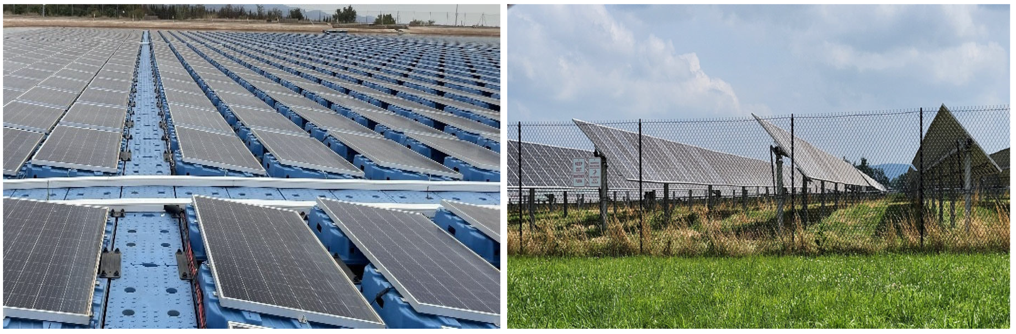
FPV systems can take on a variety of forms, but many consist of PV panels floating on buoys. These panels and buoys are in rows that have walkways dispersed throughout the system to allow for ease of access to panels for maintenance and cleaning. Some of these systems have open rack designs, allowing for space between the back of panels and the buoys (Figure 1), while others are closed. These design differences have implications on airflow below panels, which impacts PV panel generation potential given temperature differences, water evaporation, algae production, and wind resistance.
FPV systems have been deployed in over 30 different countries and are particularly favorable in areas with high population densities and high competition for land, such as Japan, Korea, and Singapore [20,21]. With the variety of deployment areas, FPV systems have been deployed in various climates and conditions, such as in arid, semi-arid, Marine West Coast, Mediterranean, and tundra like climates [22]. FPV studies from Germany, Brazil, Morocco, and Pakistan, have focused on either water evaporation effects or the capacity potential of bodies of water in the country or area of interest, and have noted benefits from FPV utilization [21,23,24,25]. While FPV has been deployed in the U.S., research on FPV systems in the U.S. context is limited. Specifically, studies in the U.S. have primarily focused on the potential of FPV systems based on either federally controlled reservoirs or “viable” human-made water bodies [26,27].
The potential benefits of FPV systems include reducing water evaporation by 25 to 50%, depending on the amount of coverage over the water body [22,24,28,29], and essentially no loss of productive farmland, as they occupy space over water bodies. This coverage also allows for better water quality, by blocking sunlight, hence reducing the occurrence of algal growth [28] that fouls irrigation equipment. FPV systems are also not visually intrusive, when compared to traditional land-based PV systems, as the embankments of the reservoir serve as a barrier to block sight of the systems in flat terrain common for the region analyzed.
As of 2015, the Grand Prairie and Cache River regions in Arkansas had 632 and 143 irrigation reservoirs, respectively, to combat declining aquifer ground water levels [30]. The reservoirs occupied 9300 and 2000 ha in those regions, respectively, with additional reservoirs likely having been constructed after the study and outside these areas. As such, the potential for FPV exists with a joint goal of (i) reducing water evaporation to increase irrigated land and thereby agricultural production; (ii) mitigating agricultural land diversion to LPV, (iii) water quality improvement with shading; and (iv) potentially reducing waterside embankment erosion from wave action.
This paper thus quantifies FPV energy generation potential, benefits of water savings, and erosion mitigation of FPV systems on irrigation reservoirs, as well as on their embankments, in the Grand Prairie and Cache River regions of Arkansas. As such, this paper focuses on quantifying FPV benefits within a U.S. subregion where irrigation reservoirs serve a critical need to supplement water needs for irrigation-intensive rice production, where Arkansas is the leading contributor for U.S. rice exports [15]. The following sections describe the methodology used and sensitivity analyses of adoption rates and water area coverage. We conclude with policy options that would make FPV a breakeven proposition relative to LPV systems given their minimal land-use cost, and lessened threat to agricultural land.

2. Materials and Methods

To calculate the potential energy generated in irrigation reservoirs from (i) FPV systems on water; and (ii) PV on their embankments, a calculator, potentially becoming available online in the future, was developed to quantify water and embankment area implications based on reservoir size, shape, and direction. Details of calculations are provided in the technical Appendix A. With surface area estimates available, the annual cost difference between LPV and FPV installations per MW of installed capacity was calculated to assess how expected benefits of lesser land leasing cost, reduced water evaporation, and embankment erosion could lessen FPV’s higher cost of installation in comparison to LPV.

2.1. FPV Area Potential Based on Reservoir Size, Shape, and Embankment Maintenance

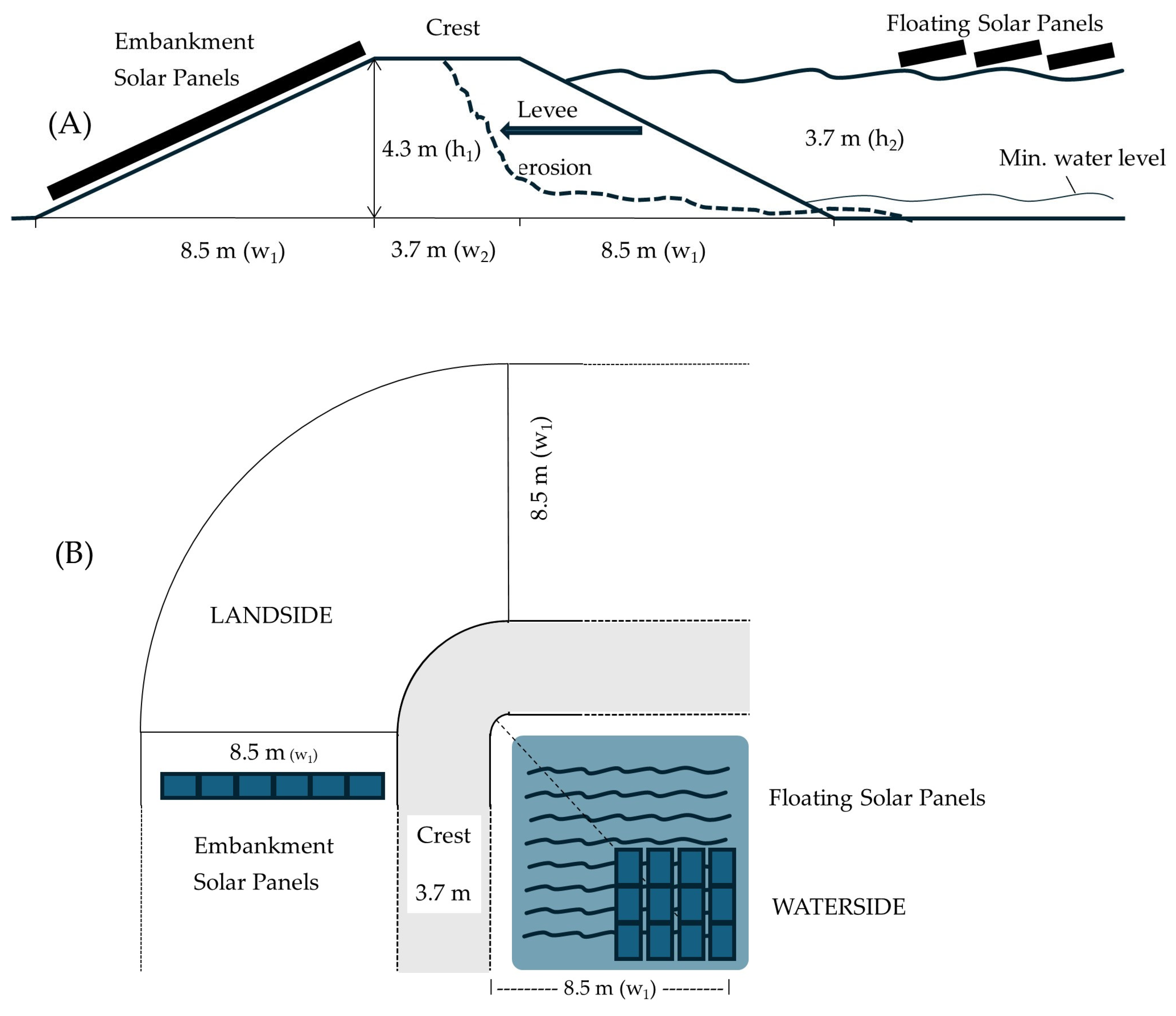
To visualize these surface area calculations on irrigation reservoirs and their embankments, Figure 2A highlights the typical cross section of an embankment constructed from soil moved from the center to the perimeter of the land area occupied by the reservoir. Wave action erodes waterside embankments over time, requiring their eventual reconstruction using tractor-drawn scrapers.
Research by Wren, Ozeren, and Reba (2016) [31] has shown that wind-induced wave erosion can lead to annual embankment maintenance costs ranging from 5.58 USD to 33.79 USD per linear m of embankment, where the range in estimates is a function of embankment slope and larger reservoirs generating larger waves. To avoid anchor interference with equipment for such reconstruction, FPV installations are expected to be anchored to the bottom of the reservoir, reducing potential surface water use to a smaller subregion available at minimum water height (Figure 2A,B).
Using 590-WDC capacity PV panels (2.28-m long by 1.14-m wide), a panel on a buoy occupies approximately 4.4 m2 assuming an additional 30 cm is added to length and width for the buoy and 20 cm for walkways and wiring (Figure 1). Using this surface use parameter of 4.4 m2 per 590-WDC panel, 1695 panels are required to reach 1 MW of production capacity, which equates to an approximate water surface area footprint of 0.75 ha/MW for FPV with stochastic modifications to that parameter explained in Section 2.6.

2.2. PV on Reservoir Embankments

Photovoltaic panels could cover south-, east- and west-facing landside slopes of embankments. North-facing panels produce considerably less energy per W of capacity in the northern hemisphere as shown in Section 4.2. Ideally these PV panels would be arranged tightly to avoid costs associated with the management of vegetation (mowing and/or trimming/removal of trees where the latter’s root systems are detrimental to the structural integrity of the embankment). Therefore, compact placement of panels to manage vegetation on embankments would lead to approximately 2.6 m2 per panel or 0.44 ha/MW. However, the possibility of wind or water erosion problems under the panels exists and is subject to further investigation. Herein, calculations account for incomplete coverage of embankment space given PV panel dimensions may not allow for full coverage of the embankment and to allot space for irrigation equipment. Hence, the area footprint per MW on embankments rests on an assumption of a minimum of 0.44 ha/MW to an ad hoc maximum of 0.56 ha/MW with an average of 0.5 ha/MW.

2.3. Aspect and Tilt of PV Panels

Breaking sections of embankment construction and embankment areas into pieces (see technical Appendix A) allowed for estimation of the water surface area that is available for FPV as well as land area for embankment PV installation. Note that aspect (compass direction) and shape of the reservoir and embankments impact exposure, intensity, and length of solar radiation and, thereby, the amount of kWh of electricity generated per kWDC of installed PV capacity. For example, a rectangular reservoir with short sides facing east and west will have more south-facing landside embankment for greater electricity generation potential than a square reservoir of the same size because south-facing panels generate more kWh/kWDC annually than east- or west-facing panels in the northern hemisphere [32,33].
To calculate annual kWh production, the NREL PVwatts calculator [34] was used to estimate output based on location-dependent solar radiation, historical weather patterns, panel aspect (cardinal direction), panel tilt angle, inverter losses, and tracking technology. For more information, please visit https://pvwatts.nrel.gov/ (accessed 12 May 2026). Effects of shading from embankments when the reservoirs are at low water levels were thought to be minor. Note that east- and west-facing panels are comparable in generation potential to south-facing ones at low tilt angles used in FPV systems (Section 3.2 and Section 4.2). A representative zip code was chosen from the Grand Prairie (72072) and the Cache River (72432) regions to calculate average annual production.

2.4. Photovoltaic Panel Specification

Annual kWh production per kW of capacity assumed a “standard” PV module type with a 19% approximate nominal efficiency and a temperate coefficient of power of −0.37%/°C. For FPV systems, a fixed rack-array type is chosen, along with a system loss percentage of 14.08%. The tilt degree chosen for the FPV systems was 6 degrees, as optimal tilt angles lower than 10 degrees for maximum light interception and minimal maintenance costs from potential wind damage are common [35]. The embankment PV systems were assumed to be mounted to the embankment surface at a typical embankment slope (27 degrees). Different aspects (south, east, and west) for both FPV, LPV, and embankments were investigated and are discussed in Section 4.2.

2.5. Number, Location, and Shape of Reservoirs

The average reservoir size in the Grand Prairie and Cache River regions is approximately 14.6 and 20.2 ha, respectively, and ranges from 1 to 265 ha [30]. To simplify, we assume an average reservoir size of 16.2 ha. An embankment height of 4.3 m with a typical 2:1 ratio embankment slope and 3.7-m crest (Figure 2). With rectangular reservoirs, a length-to-width ratio of 3:2 was used with the longer sides facing south and north. Finally, a minimum water level of 0.3 m, along with a maximum water level of 3.7 m, allowed calculation of surface area for FPV and embankment PV systems.
The reservoirs that are present in the Grand Prairie and Cache River region come in all shapes and sizes, with some being square, rectangular, or even irregularly shaped. While simple shapes, square and rectangular, are cheaper to construct than irregular-shaped reservoirs, the latter exist as previous bodies of water may have been incorporated into a new system or used as is with minimal embankment construction. Notably, the shape of a reservoir will not impact the sizes of FPV systems significantly, as their design is modular, but likely impacts anchoring costs and embankment PV installation. Such details are considered site- rather than region-specific and thus are only mentioned rather than accounted for specifically in this study.

2.6. Cost Differences Between LPV and FPV

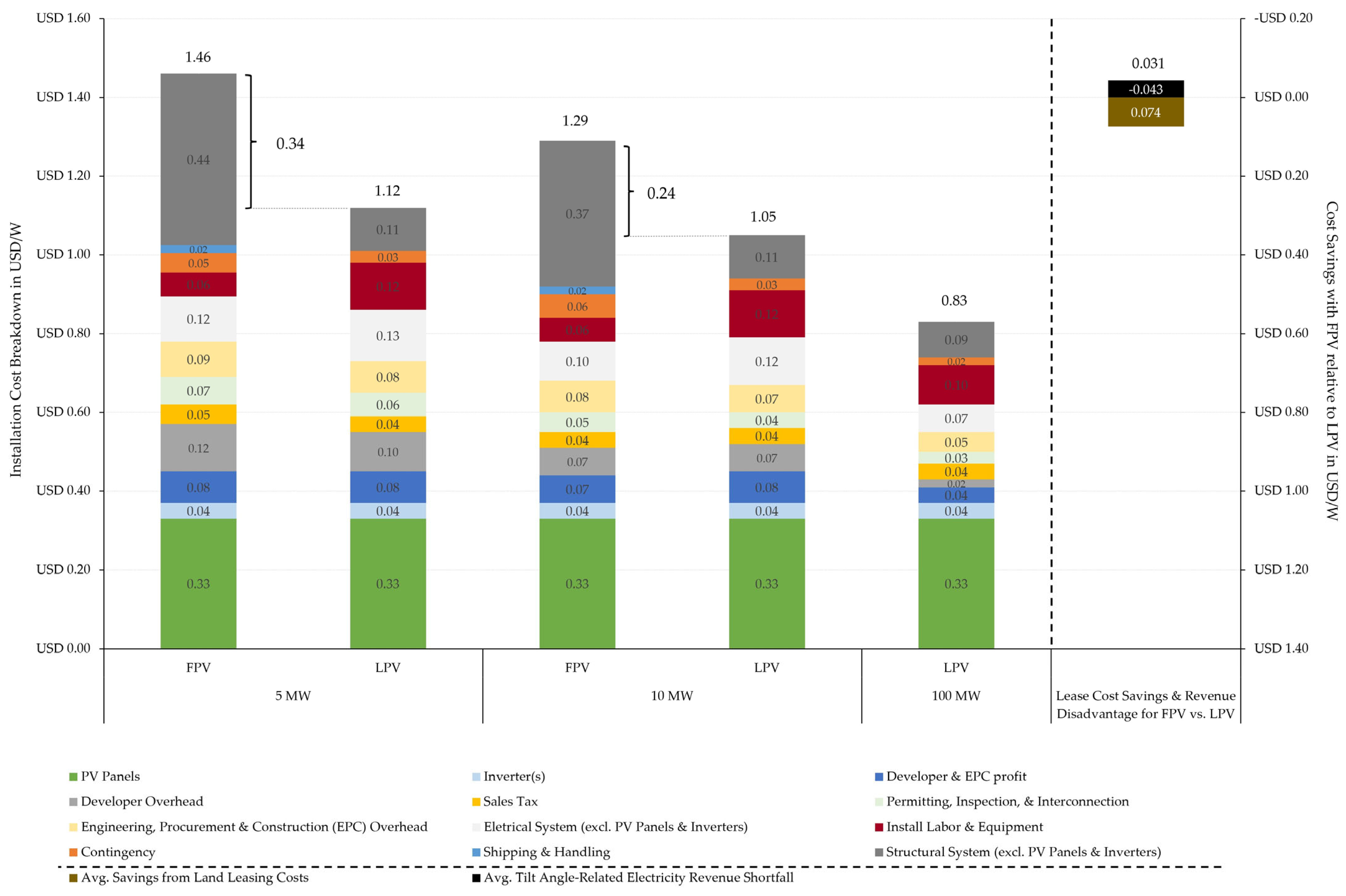
LPV systems are documented to cost approximately 0.24 USD/W less than FPV systems at the 10-MW system size, and 0.34 USD/W less at the 5-MW system size, (Figure 3) according to an NREL report by Ramasamy and Margolis (2021) [36]. Since large utility-scale LPV systems (100-MW+) are the most cost effective, they were also considered for comparison against FPV installations, with a cost that is approximately 0.63 USD/W and 0.46 USD/W less than 5-MW and 10-MW FPV installations, respectively (Figure 3).
At 0.9 ha/MW, the average of our calculations from Section 2.1 and Lopes et al. (2020) [13] for an FPV system, both the 10-MW and 5-MW size options are feasible for a typical 16.2-ha reservoir but lead to different water surface use.
Figure 3. Difference in cost per Watt (W) at the time of installation for land-based (LPV) and floating PV arrays (FPV) at the 5-MW and 10-MW system sizes (left scale) as reported by Ramasamy and Margolis (2021) [36] and Ramasamy et al. (2021) [37]. Present value of annual lease cost savings and revenue difference associated with FPV vs. LPV installation over 30 (± 4)-year useful life (right scale). Water savings and reduced reservoir maintenance benefits are reflected in the lease cost differential between LPV and FPV as shown in Figure 4. Dashed line differentiates use of right-hand axis in the graph and legend.
Energies 19 02646 g003
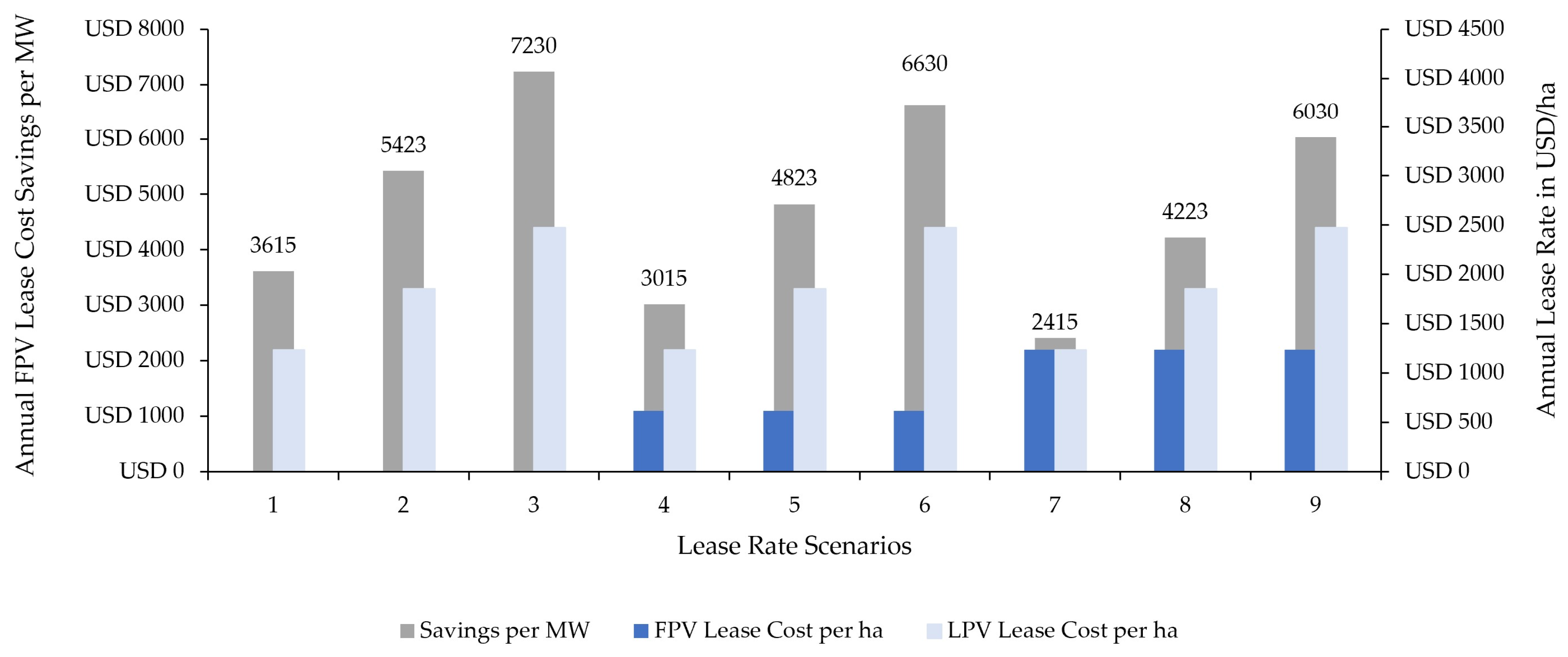
Figure 4. Annual savings on land leasing cost per MW for floating PV panels (FPV) compared to land-based PV panels (LPV) for the three lease rate scenarios for each of FPV and LPV using 0.98 ha/MW for FPV and 2.93 ha/MW for LPV.
Energies 19 02646 g004
Regardless of technology, we estimate project lives to vary between 24 and 36 years with a mode of 30 years using a triangular distribution, as inverter replacement in 12-year intervals is common. Longer project lives are possible. With PV technology, a relatively mature industry, we utilize discount rates ranging from 3% to 7% with 5% as the modal interest rate, again with a triangular distribution. Monte-Carlo simulation surrounding these parameters allowed estimation of 90% confidence intervals (reported in parentheses throughout) following our point estimates using @Risk v 7.6.1, Palisade Corp.: Ithaca, NY, USA [38], assuming no correlation between uncertain parameter estimates using 10,000 iterations.

2.7. Lease Cost, Water Evaporation, and Embankment Erosion Mitigation Savings

While installation costs between FPV and LPV systems differ, FPV can provide several cost savings. These savings include avoided water evaporation due to shading, leading to greater irrigation capacity per reservoir, and embankment erosion mitigation. FPV also occupies less area compared to LPV systems, leading to lower land lease costs for developers. Reduced water evaporation and erosion mitigation can be considered private benefits to the producer, or owner of the reservoir, while the lease cost savings are captured by the developer. The savings generated for the producer may lead to lower lease rates for water bodies compared to agricultural land. We quantify water evaporation cost and erosion mitigation savings below to provide information to both developers and reservoir owners; however, we reflect only leasing cost changes to avoid double counting. Because leasing rates depend on many factors (e.g., proximity to load demand, electric grid infrastructure, and alternative uses for irrigation reservoirs), we employ nine scenarios for land lease cost savings (LCS):
L C S ¯ = j = 1 k (   A R L P V · L R L j A R F P V · L R W j ) / k
where A R L P V and A R F P V are previously mentioned average land use efficiencies of 2.93 and 0.9 ha/MW, respectively, and L R L j and L R W j are annual lease rates for agricultural land vs. water bodies/embankments for j = 1 … k scenarios (k = 9). Conservatively, we varied L R L between 1236 USD, 1853 USD and 2471 USD/ha, with the lower end of lease rates in comparison to the 1100 USD–6200 USD/ha range mentioned above, in anticipation of future competition from FPV installations. Research to ascertain greater precision surrounding these estimates were in early stages at the time of this analysis. At the same time L R W at zero, 618 USD and 1236 USD/ha, were considered potential lease rates considering a producer would factor in anticipated water evaporation savings and potential for less embankment maintenance detailed below. Despite this ad hoc estimation of LCS, a normal distribution was fitted to these nine scenarios to allow calculation of a confidence interval for this range of estimates. We aggregate these savings over the modal useful life of the systems, n = 30, using a modal discount rate, i = 5%, and an ordinary annuity factor, [1 − (1 + i)n]/i, to arrive at the present value of L C S ¯ per MW such that the accumulated value of annual L C S ¯ could be compared to installation cost differences between LPV and FPV.
Second, evaporation reduction, due to lower free water surface evaporation from shading from the floating PV panels, provides a producer benefit that adds to the value of FPV. If a 50% reduction in evaporation occurs, as much as 23.6 ha-cm of water can be saved with floating panels on irrigation reservoirs, as water bodies in Arkansas lose approximately 47.3 ha-cm of water from evaporation [39]. On the one hand, such evaporation losses translate to cost savings from avoided relift charges, as water lost to evaporation does not need to be pumped into the reservoir. On the other hand, the added available water, assuming producers minimally refill the reservoir during the growing season, will lead to more pumping costs to irrigate additional land. This leads to a zero-sum game in terms of relift charges but does lead to more land that can be irrigated from water savings.
Using a range of 25 to 50% reduction in evaporation (or a modal 37.5% of 47.3 ha-cm with a triangular distribution) due to FPV coverage mentioned above [28,29], approximately 17.7 ha-cm (±4.0) per ha of PV panel water coverage are saved during the crop production season. At 0.9 (±0.1) ha/MW, approximately 16.0 (±4.2) ha-cm of water evaporation loss avoidance is expected per MW. With the average water use of common crops grown in the region for flood-irrigated rice using either contour, straight, or zero-grade levees reported at 26.7 ha-cm, and furrow-irrigated corn and soybeans requiring from 13.4 to 13.9 ha-cm per season, respectively, the additional available water translates to 0.60 (±0.16) or 1.17 (±0.31) ha of additional irrigated rice or soybean per MW capacity, respectively [40,41,42]. With a 2-yr rice/soybean crop rotation, common in the production region analyzed [43], the aforementioned 245 USD/ha cash rent difference between irrigated and non-irrigated agricultural land thus translates to 50% of 0.60 (±0.16) ha added irrigated rice and 50% of 1.17 (±0.31) ha added irrigated soybean or an annual average value of 217 USD (±56)/MW for water evaporation savings that helps offset the installation cost difference between LPV and FPV:
{ 217   USD MW   ·   [ 1 ( 1   +   i ) n ] i } 1,000,000   =   0.0033   USD   ( ± 0.0011 )   per   W   of   generation   capacity
Alternatively, if producers do refill the reservoir during the irrigation season, or have wells to draw groundwater, additional irrigated land is not a realistic scenario. Even if this is so, FPV still offers savings in the form of cheaper pumping costs. Using information from McDougall (2015) [44], the energy cost of pumping water from ground water sources (assuming 45.7 m depth to water) and drawing it out of the reservoir (assuming 5.5 m relift over the embankment) is 2.99 USD and 0.54 USD per ha-cm, respectively. We ignore repair and maintenance, labor, and equipment ownership charges, as they are assumed the same for both groundwater and reservoir sources. Therefore, an average water evaporation reduction of 16.0 (±4.2) ha-cm/MW valued at the pumping cost differential of 2.99 USD vs. 0.54 USD per ha-cm translates to cost savings of 39 USD (±10)/MW. Replacing the 217 USD estimate with 39 USD in Equation (2) thus leads to fewer producer cost savings. This translates to a scenario where the producer would require a higher lease rate for FPV on their reservoir.
Lastly, when considering embankment erosion mitigation from wave action, a range of annual embankment maintenance costs of 5.58 USD to 33.79 USD per linear m of embankment (modal and average 19.69 USD/m using a triangular distribution) and an average inner circumference of a 16.2-ha reservoir of 1528 m were used (With a 50/50 split of square/rectangular reservoirs, the average outside perimeter (L1 and L2 per Appendix A), subtracting 24.4 m for outer embankment and crest, leads to an average inner embankment circumference at max water height of 1519 (±15 m) using a uniform distribution with max. and min. inner circumference for rectangular and square shapes, respectively). Wren, Ozeren, and Reba’s (2016) study [31] showed approximately 1350 m3 of soil erosion from wind and wave action on waterside embankments over seven months and 1530-m length of embankment in Arkansas. Prorated to 12 months, approximately 2313 m3 of soil needs to be rebuilt on levees without wave abatement. While wind erosion cannot be mitigated by the presence of FPV systems, wave-induced erosion can be, as wave abatement with the FPV’s flotation system has been studied. Gomis et al. (2026) [45] noted that for wavelengths shorter than 9 m, FPV systems can dissipate up to 96 percent of their energy, leading to less soil erosion on waterside embankments. With this in mind, we assume a 15% reduction in maintenance costs (with an ad hoc range of 5–25% using a triangular distribution) from wave energy dissipation. Using the 0.9 (±0.1) ha/MW of FPV and 13.08 (±0.03) ha of available surface water area pending shape, we prorate embankment erosion benefits of different-sized installations (or water surface coverage) on a per MW basis such that annual maintenance savings amount to:
6.9 ( ± 0.8 ) % / reservoir / MW   ·   ( 15   ( ± 7 ) % · 19.69   USD   ( ± 9.64 ) m · 1519 ( ± 15 )   m reservoir )   =   310   USD   ( ± 234 ) / MW
or a present value of 0.48 ( ± 0.37 )   cents per W of capacity over the 30 (±4)-year useful life, using Equation (2). With the reservoir maintenance cost calculation based on a 2016 study, these calculations are likely conservative given inflationary pressure since then.
At the same time, optimal configuration of modular FPV within a reservoir to both minimize embankment erosion and maximize system performance is considered beyond this study’s scope. For example, anchoring panels around the perimeter of the water surface area may cover only a small percentage of the reservoir but provide large erosion benefits, likely using inefficient anchoring with large amounts of wiring in comparison to a block of panels (covering the same amount of water) but arranged as a square in one corner or side of the reservoir with less anchoring and wiring expenses but also less expected wave reduction.

2.8. Sensitivity Analyses

To account for varying levels of adoption of FPV, since maximum PV panel coverage over all reservoirs in the two regions is not expected, we investigated 20 different adoption rate scenarios. We present five different percentages of FPV water area coverage by PV panels per reservoir, as well as four different adoption rates of producers allowing installation of FPV on their reservoirs (i.e., number of reservoirs) by investors or on their own in the Grand Prairie and Cache River regions. The percentages of available water surface covered by PV panels per reservoir ranged from 5, 15, 25, 50, and 80% (top to bottom of Table 1) of the water surface in a reservoir at its minimum water level (Figure 2). We further employed 4 different investor adoption rates or percentages of reservoirs investing in FPV to range from 10, 25, 50 and 100% of reservoirs in each respective region (left to right in Table 1).

3. Results

3.1. Overcoming Cost Differential Between LPV and FPV

As presented above, FPV installations are more expensive per MW capacity than LPV (Figure 3). The right-hand column in Table 1 indicates the size of system (in MW) per reservoir under different water surface utilization scenarios. As noted in Nobre et al. (2024) [46], FPV installations are highly variable in water coverage rates (<1–~90% on freshwater bodies with an approximate average and standard deviation of 34.2 and 22%, respectively. Together with embankment electricity generation capacity, system sizes between 5- and 10-MW (approximately 25% and 50% water coverage, respectively) are thus likely candidates. For those size installations, the installation cost disadvantage of FPV vs. LPV ranges from 0.34 USD to 0.24 USD/W (Figure 3).
Using the L C S ¯ from Equation (1), or the average of the nine LCS scenarios depicted in Figure 4 as the numbers above the gray bars, an average annual savings of 4822.50 USD (±1649.33 USD Std. Dev.) per MW was determined (Section 2.7).
These annual lease cost savings translate to an equivalent, one-time present value of 0.074 USD (±0.014)/W (Figure 3) over the modal 30 (±4)-year useful life using:
{ 4822.5   USD MW   ·   [ 1 ( 1   +   i ) n ] i } 1,000,000   =   0.074   USD   ( ± 0.014 )   per   W   of   generation   capacity
Recall that these LCS for solar developers are in part a result of cost savings to producers in the form of reservoir maintenance and the higher of water savings estimates that are 16 to 22 times smaller in comparison to L C S ¯ (see Equations (2)–(4)). This is to say, a producer expecting more/less water savings or maintenance cost reductions than what was calculated above may be willing to lease their reservoir for less/more, respectively. As such, we stipulate that negotiated lease rates for reservoirs capture or monetize water savings and maintenance cost reductions.
With the above cost savings of 0.074 USD (±0.014)/W for developers employing FPV in comparison to LPV, installation cost differences for 5- and 10-MW systems thus drop from 0.34 USD and 0.24 USD/W to 0.26 USD and 0.16 USD/W on average, respectively (Figure 3). The same can be said in comparison to large-scale utility LPV installations (100-MW+) and 5-MW and 10-MW FPV systems, where the difference drops from 0.63 USD/W to 0.55USD/W and 0.46 USD/W to 0.38 USD/W on average, respectively (Figure 3).

3.2. Valuing Tilt Differential Between LPV vs. FPV

As discussed in Section 2.4, tilt angle differs between LPV, FPV, and embankment PV. As such a kWDC of installed annual capacity will not yield the same amount of annual kWh. Using the PV Watts tool [34] and their point and range estimates as the mode, minimum and maximum to employ skewed triangular distributions of annual kWh/kW by Zip-code and tilt angle, we could estimate annual revenue differences by system. To inform the reader about electricity generation efficiency differences by tilt angle and panel orientation, we present this information for S, E, W, and N facing panels in Table 2. Using this information, we calculate the PV of system lifetime annual revenue stream differences across system technologies using a skewed triangular distribution for electricity value generated with an avoided cost rate as the minimum (0.02 USD/kWh [47]), 0.03 USD/kWh for the mode, and industrial electricity rates as the maximum (0.05 USD/kWh [48]). We expect FPV investment by utilities and as such hypothesize that they value electricity at avoided cost or the price they would need to pay from alternative sources.
Using south-facing FPV and LPV kWh/MW valued at an average of 3.33 (2.38–4.45) cents per kWh, the PV revenue advantage with LPV vs. FPV amounts to a one-time cost disadvantage for FPV of 0.043 USD (0.021–0.070)/W over a 30 (±4)-yr useful life on average across both regions. This, accordingly, lowers the cost savings of FPV (from LCS) or 0.074 USD (±0.014)/W by the revenue disadvantage of 0.043 USD (0.021–0.070)/W to 0.031 USD (0.004–0.055)/W.

3.3. Implications at the Household Level

Given that one W of capacity can produce an estimated average of 1.331 (1.304–1.357) kWh/W per year (Table 2, average of south-facing FPV in the Grand Prairie and Cache River regions) and the 30 (±4)-yr useful life of these systems, the one-time 0.31 USD (0.005–0.055)/W cost disadvantage of FPV over LPV translates to an upcharge of approximately 0.77 (0.66–0.92) cents/kWh once spread over 30 years for 5-MW sized systems. Dividing the 0.031 USD (0.004–0.055)/W cost difference by 1.331 (1.303–1.357) kWh/W leads to the installation cost difference that can be further divided by the 30 (±4)-yr useful life of the systems to arrive at the annual 0.77 (0.66–0.92) cents/kWh for FPV over LPV. Similarly, the cost advantage amounts to 0.52 (0.43–0.64) cents/kWh for 10-MW systems. For the average household, which currently sources less than 5% of their electricity from PV, annual cost implications of FPV vs. LPV thus amount to:
5 %   · 12,000   kWh household · 0.0077   ( 0.0066 0.0092 )   USD kWh   =   4.64   USD   ( 3.93 5.51 ) / household
more with FPV than LPV at the 5-MW system size or 3.13 USD (2.58–3.82) with 10-MW systems. If comparing the 100-MW LPV system to a 5-MW FPV system, the 0.60 USD (0.58–0.62)/W cost disadvantage translates to 1.50 (1.30–1.75) cents/kWh, or an upcharge of approximately 8.99 USD (7.81–10.52) per household annually.
While Table 1 provided insight into PV electricity capacity expansion possibilities with FPV, Table 3 translates these findings to annual electricity production in GWh per 16.2-ha reservoir to get a sense of expansion in availability of annual electricity. Further detail on region-specific differences in PV generation potential is discussed in Section 4.2. At 25% of water coverage, or 4.45 (±0.48)-MW capacity, approximately 6 GWh are available when south-facing embankments are covered. That would provide sufficient electricity for 500 households per 16.2 ha reservoir with a 5-MW FPV system.

3.4. Water Savings

Water evaporation savings are highlighted in Table 4. While these savings are relatively small per reservoir, they do add up when aggregating across the many reservoirs in use. Recall that ~800 reservoirs were in use in the regions analyzed in Arkansas as of 2015 [30].

4. Discussion

4.1. Rationale for Encouragement of Embankment PV and FPV

The reasoning for policy intervention stems from citizen concern over loss of agricultural land from LPV systems and the potential effect it may have on food security and the state economy. The Arkansas Advanced Energy Association predicts that an energy crisis can begin in Arkansas as early as 2026 and the shortage could grow to 3891 MW by 2035 if nothing is done to address it [19]. With utility-scale LPV a cost-effective, technologically mature, and sustainable energy production solution that generates electricity during high-demand periods of the day, using the 2.93-ha average per MW of capacity, employing LPV would lead to a need for approximately 11,400 ha of land. Assuming 5% of the electricity shortage is met with LPV, 570 ha of agricultural land is at risk of being converted. Based on average yields in Arkansas, ~4900 mt of rice, ~6700 mt of corn, or ~2100 mt of soybeans would be lost [49,50,51].
Focusing on rice as a food staple, as Arkansas is the top rice producing state in the U.S., losing this amount of crop would generate a producer revenue loss of approximately 1.5 million dollars annually when valued at 0.31 USD/kg [49]. With a milled rice yield of 60%, an ~3000 mt loss in milled rice production translates to a loss of 30.8 million meals annually, if the average portion of dry rice in a meal is 95 g (1/2 cup).
If FPV was utilized instead to cover this potential energy gap, it would only require approximately 3500 ha at the 0.9 ha/MW average without crop loss. In fact, it could increase food production due to an increase in irrigated acreage from water evaporation savings. Other benefits that come from FPV use are intangible. Citizens may like the idea that FPV systems are less visible than LPV ones, as they would be in rural areas hidden within reservoirs. Producers may prefer FPV because they can still receive lease payments for PV, while not giving up any land, and they can potentially receive more time to plan and save for the repair of irrigation embankments from mitigated wave erosion. Another justification for subsidizing FPV installations in Arkansas is that it could have positive impacts on communities in terms of job creation. In 2023, jobs in the renewable energy sector grew more than twice the rate of the U.S. labor market as a whole [52].

4.2. Policy Options for Incentivizing FPV over LPV

The first policy option presented herein is the use of renewable portfolio standards (RPS). Many countries as well as states within the U.S. have enacted RPSs in response to the demand for a transition to renewable energy sources from fossil fuels. RPSs are requirements, or in some cases simply goals, for the amount of energy that comes from low- or zero carbon-emitting sources [53]. Many RPS programs utilize a credit trading system to measure how much renewable energy is generated or purchased from distributed generators to track compliance [53]. Some of the funds that are generated from RPS compliance go to investment in renewable energy sources, producing an opportunity for FPV installation funding.
Research has shown that RPSs are effective in reducing carbon emissions but can lead to higher energy costs for consumers if compliance costs are high [38]. However, if compliance costs are too low, then there may not be enough funds to properly subsidize renewable energy development [54]. These programs can lead to higher electricity prices because of the issue of inconsistent energy generation posed by renewable energy sources, meaning that investments into batteries for excess energy produced during peak hours need to be made [55]. Increased electricity prices are also contingent upon whether the cost of renewable energy sources falls faster than electricity produced from fossil fuels [55]. It is important to note that a recent report by the EIA shows that solar PV installations can have a lower levelized cost of energy (LCOE is the cost of generating energy for a particular system [56]) (LCOE) in comparison to sources such as natural gas-fired combined-cycle, advanced nuclear, hydroelectric, and offshore wind, even without a tax credit (With and without a tax credit, onshore wind has a lower potential LCOE than solar PV [41]) [57]. This suggests that a rise in electricity prices is not a given when utilizing an RPS.
It is also important to note that when utilizing an RPS, policy design is essential in capturing preferred outcomes. Bhattacharya, Giannakas, and Schoengold’s (2017) [58] research suggests that changes in consumer and producer welfare from an RPS are case-specific. Variables, such as consumer preference for renewable energy power, the impact of RPS subsidies on renewable energy generation, and the degree of competition among power suppliers, play a role in determining how much both parties gain or lose and differ from case to case.
Arkansas does not currently utilize an RPS, and its enactment could potentially lead to the rise of FPV use in irrigation reservoirs, as utility companies would be expected to expand renewable energy sources. If citizens do not want to see more agricultural land transition to PV panel fields, they could pay a premium, ranging on average from 3.13 USD to 8.99 USD per household annually (Equation (5)), or the difference in cost associated with FPV and LPV installations pending system size comparison, to support the development of FPV to reach RPS requirements or goals.
An EIA report from 2023 shows that the average monthly electricity bill for Arkansans was 128.51 USD [59], meaning consumers’ bills would increase as much as 0.7% if the maximum estimated cost difference between FPV and LPV was passed on to them. It is important to note that the percentage of PV energy consumed may increase as more energy is produced with the utilization of FPV, but as mentioned previously, the cost of solar PV is decreasing faster than most sources.
Alternatively, or in conjunction with an RPS, Arkansas can look to directly subsidize FPV installations and the energy they produce. To make the cost of FPV and LPV installations similar in cost, the aforementioned average 3.13 USD to 8.99 USD per household per year could be charged as a fee and redistributed to FPV developers to discourage LPV investment. Further, this fee could be charged to consumers only where FPV installations create energy.
Subsidizing the adoption of new technology has been shown to spur investment in new technology [60,61,62]. Even if the subsidy is a one-time cash contribution to increase technology awareness, it may be effective, as it allows investors to try the technology at a lower risk [62].
The federal government already has several different tax credit programs that incentivize the construction of PV energy projects. These programs include the investment tax credit (ITC) and production tax credit (PTC) [63]. The ITC reduces the tax liability for a percentage of the cost of a PV system, while the PTC is a per kWh tax credit awarded for the first 10 years of a system’s operation [63]. If an FPV installation was to utilize the ITC, the cost gap between FPV and LPV declines, as FPV has a higher upfront installation cost leading to a greater investment tax credit. There is also an opportunity to limit the ITC and PTC programs to just FPV installations, which would serve to not only preserve federal government resources, as more restrictions are placed and therefore fewer projects can be funded, but also make FPV installations more appealing than LPV.
Other opportunities for federal funding for FPVs can come from the Environmental Quality Incentive Program (EQIP) and/or the Natural Resources Conservation Service (NRCS). These grants could be utilized due to expected water-saving and water-quality improvements available from FPV utilization, and if combined with the ITC or PTC could make these systems palatable to developers and/or producers.
Providing subsidies for FPV does come at a cost, usually in the form of raised taxes, or a reallocation of funds from other programs. Similar to RPSs, case-specific attention to total welfare implications for a community would be better informed via surveys or community meetings to determine the value of preserving agricultural land while increasing renewable energy production. Therefore, these mechanisms for encouraging FPV installations should be viewed as exploratory rather than prescriptive. It should also be noted that, while FPV installations can mitigate carbon emissions, they can contribute to non-carbon greenhouse gas emissions. This is due to the non-carbon greenhouse gas emissions related to PV production. This means that non-carbon greenhouse gas emissions can be outsourced to PV production areas for PV technology purchasers [64]. Such program leakage can thus lead to unintended emissions that should be considered prior to investment, especially if carbon mitigation is considered when making decisions on FPV utilization.
When thinking about how to maximize the benefit of FPV incentives, placing a priority on one of the locations may be necessary. As the results from the PVwatts calculator [34] in Table 5 suggest, the Grand Prairie region has slightly higher productivity compared to the Cache River region. Also, FPV has less kWh/m2 of surface area given panel spacing (Figure 2) needs for walkways and wiring in comparison to compact placement of embankment panels. However, FPV fairs well against LPV given greater spatial density.
While the efficiency difference across regions within a system technology is minimal, such differences increase as the installation size increases. Also, larger reservoirs could be targeted first, as they allow for economies of size to lower the cost difference for FPV when compared to LPV systems (Figure 3). For smaller reservoirs, larger coverage of the water surface area could also be a target but may meet with resistance as more habitat for wildlife would be affected.
Another consideration is the orientation of the panels within the reservoir, as well as the embankments. The results from Table 5 support the consensus that panels in the northern hemisphere benefit from facing south, as it can increase energy output. However, that does not mean that subsidies should only target south-facing installations. As seen in Table 5, since the tilt angle of the FPV installations is low, the difference in generation potential between south-, east-, and west-facing panels is minimal. East- and west-facing panels capture morning and evening sunlight more effectively than south-facing panels [32]. This means that the decision on panel aspect can be dependent on when energy is most needed.
When thinking about embankment installations exclusively, the south- vs. east-, and west-facing choice is clearer. As the tilt angle of panels increased, so did the disparity in energy generation potential between south-, east- and west-facing panels. What is interesting is the choice between the shape of the reservoir. When considering rectangular reservoirs where the long sides are facing north and south, as seen in Table 1, south-facing panels on rectangular reservoirs are preferred over south-facing panels on square-shaped reservoirs. When considering the timing of energy generation, the opposite is true, as the focus may shift to include east- and west-facing panels. Irregular-shaped reservoirs are hard to account for when determining embankment PV systems because their sides may include south-east or south-west aspects, for example. Also, reservoir embankment installations may be considered exclusively by producers, as they can use the energy produced to offset operating costs for irrigation equipment such as pumps. They are also cheaper to install and therefore may be preferred for producer use, while leaving FPV systems on reservoirs to developers and solar PV leasing arrangements. Greater detail on this aspect should be part of site-specific feasibility studies but is considered beyond the scope of this study.

4.3. Industry Focus for FPV Installation Costs

As noted in the report by Ramasamy and Margolis (2021) [36], the largest cost for FPV systems is buoys for the PV panels and their anchoring and mooring systems. They add a 300% increase in structural costs compared to LPV systems, at the 10-MW size. If FPV developers want to increase the viability of FPV in comparison to LPV systems, this cost may well be the one to target for efficiency gains. Even decreasing the difference by 0.05 USD per W for installations at the 10-MW size would decrease the annual cost disparity between FPV and LPV substantially.

4.4. Limitations

There are limitations to the calculations made in this paper. One of these limitations is related to locations used within the PVwatts calculator [34]. Only one zip code was chosen and used for each region, which may not be a good representation, especially considering that the Grand Prairie and Cache River regions span multiple counties. This means that there is a chance for more variance than the average presented. It should also be noted that not every reservoir within the Grand Prairie and Cache River region may be appropriate for FPV systems. This could be due to geological constraints, or lack of utility infrastructure. Reservoirs that are in more remote areas of the Grand Prairie or Cache River region may not have the grid infrastructure to handle a large influx of electricity.
Reservoir length and area calculations (Appendix A) that were used also present limitations, as they only account for rectangular and square-shaped reservoirs. While FPV installations are modular and can be made to fit many shapes, the embankment PV systems would face different challenges when being installed on an irregularly shaped reservoir. Further, the calculations used only consider mono-crystalline or polycrystalline cell technology instead of others such as perovskite or thin-film because of lack of a consistent data availability on cost estimates for system installations and current dominance of market share of mono-crystalline or polycrystalline cell technology. Further study of perovskite technology is thus considered subject to further research. Another limitation that may well be subject to further research is the impact of FPV installations on waterfowl. This research did not account for the impact of how lesser water surface area may affect waterfowl, especially considering the two areas of interest are within the path of migratory birds.
Finally, lesser or higher-capacity PV panels of varying dimensions impact space use efficiency, electricity generation, and cost and could have been used for this analysis. Such stipulations are left for further site-specific analyses.

5. Conclusions

FPV systems on irrigation reservoirs with PV on the embankments in the Grand Prairie and Cache River regions of Arkansas present an opportunity to generate mass PV energy with minimal to no cost of agricultural land use. The mass energy generation potential is highlighted by the fact that several adoption scenarios presented matched or exceeded current electricity generation within Arkansas as of 2025. It is important to note that FPV installations do come at a higher cost than traditional LPV installations, but the gap closes as both systems grow in size. Considering lease cost savings were insufficient to offset this cost differential, policy intervention using an RPS, state level subsidies, and continued federal investment tax credits can be tools to mitigate further agricultural land use diversion to PV. Nonetheless, benefit estimates of FPV are preliminary and require on-farm validation through pilot FPV installations. As such, a phased approach starting with demonstration projects is likely warranted before large-scale deployment. Research into lowering the cost of floatation and anchoring systems may also help make FPV more cost-competitive with LPV. All options discussed present their own unique benefits and challenges. A mixture of them may well be optimal from a consumer, solar developer, farmer, and water conservation perspective. Finally, the 8.99 USD (7.80–10.54) per household (max. +0.7% of annual electricity bills) estimate compared a 5-MW FPV to 100-MW LPV which could be considerably smaller with the deployment of larger FPV installations.

Author Contributions

Conceptualization, M.P., T.W., Y.L., and C.H.; methodology, T.W. and M.P.; validation, T.W., M.P., C.H., Y.L., and A.D.-M.; formal analysis, T.W. and M.P.; investigation, T.W. and M.P.; resources, M.P.; data curation, T.W. and M.P.; writing—original draft preparation, T.W.; writing—review and editing, M.P., Y.L., A.D.-M., and C.H.; visualization, M.P. and T.W.; project administration, M.P. All authors have read and agreed to the published version of the manuscript.

Funding

Popp received funding from the Arkansas Agricultural Experiment Station, Hatch Project number 2925.

Data Availability Statement

Data used in this study will be available upon request.

Acknowledgments

The authors would like to thank Miguel Redón Santafé, Rural and Agro-food engineering at Polytechnic University of Valencia, and Douglas Hutchings of Delta Solar, for their thoughtful feedback and comments during the editing process.

Conflicts of Interest

The authors declare no conflict of interest.

Abbreviations

The following abbreviations are used in this manuscript:
PVPhotovoltaic
LPVLand-based utility-scale photovoltaic systems
FPVFloating photovoltaic systems
EQIPEnvironmental Quality Incentive Program
NRCSNatural Resources Conservation Service
RPSRenewable Portfolio Standard

Appendix A

Reservoir area calculations for water surface area at minimum water level and embankment surface area.
With a square reservoir, the lengths of the sides (L1 = L2) in m are:
L 1   =   L 2   = R A × 100
where RA is the land footprint of the reservoir in ha (including the embankment). For a rectangular reservoir, the length of sides depends on the length-to-width ratio (WR) as follows:
L 1 = R A W R m i n W R m a x × 100   and   L 2 = R A W R m a x W R m i n × 100
where WRmin and WRmax are the smaller and larger values, respectively of the length-to-width ratio of the rectangle and L1 and L2 are the long and short sides of the rectangular perimeter of the reservoir (water body and embankment).
The length and width of the water body are determined using the following equations (Figure 2):
Length of water body at maximum water level:
L m a x   = L 1 2 ( w 1 + w 2 + s ( h 1 h 3 h 2 ) )
Width of water body at maximum water level:
W m a x   = L 2 2 ( w 1 + w 2 + s ( h 1 h 3 h 2 ) )
where w1 is the base of the landside or waterside embankment, w2 is the width of the crest, h1 is the height of the embankment, h2 is the water level at maximum and minimum fill, h3 is the minimum water level fill and s is the embankment width-to-height ratio or the inverse of the slope.
As such, the length and width of the water body at the minimum level are:
L m i n   = L m a x s × 2 h 2   and   W m i n   = W m a x s × 2 h 2
These calculations are used to determine the water surface area at both the maximum and minimum water level.
Embankment area (A) takes the length of the reservoir facing south, east, or west pending aspect of the reservoir using the outside perimeter length (L) as well as embankment width (W) into consideration:
A   =   [ L     2 ( w 1 + w 2 ) ] × w 1 2 + h 1 2

References

  1. Pourasl, H.H.; Barenji, R.V.; Khojastehnezhad, V.M. Solar Energy Status in the World: A Comprehensive Review. Energy Rep. 2023, 10, 3474–3493. [Google Scholar] [CrossRef]
  2. EIA. What is U.S. electricity generation by energy source? U.S. Energy Information Administration. February 2024. Available online: https://www.eia.gov/tools/faqs/faq.php?id=427&t=3 (accessed on 17 June 2025).
  3. Antonio, K. Solar and Wind to Lead Growth of U.S. Power Generation for the Next Two Years—U.S. Energy Information Administration (EIA). EIA. 16 January 2024. Available online: https://www.eia.gov/todayinenergy/detail.php?id=61242 (accessed on 27 May 2026).
  4. SEIA. State Solar Spotlight: Arkansas. Report. SEIA/Wood Mackenzie Power & Renewables Solar Market Insight. Solar Energy Industries Association. 2025. Available online: https://seia.org/solar-state-by-state/ (accessed on 22 October 2025).
  5. EIA. Arkansas State Profile and Energy Analysis. U.S. Energy Information Administration. July 2024. Available online: https://www.eia.gov/state/analysis.php?sid=AR (accessed on 17 June 2025).
  6. Ember. Share of Electricity Generated by Solar Power. Data compiled from Energy Institute, Statistical Review of World Energy (2025), with major processing by Our World in Data. 2026. Available online: https://ember-energy.org/data/electricity-data-explorer/ (accessed on 15 May 2026).
  7. Bolson, N.; Prieto, P.; Patzek, T. Capacity factors for electrical power generation from renewable and nonrenewable sources. Proc. Natl. Acad. Sci. USA 2022, 119, e2205429119. [Google Scholar] [CrossRef]
  8. EIA. Southwest states have better solar resources and higher solar PV capacity factors. EIA. U.S. Energy Information Administration. 12 June 2019. Available online: https://www.eia.gov/todayinenergy/detail.php?id=39832 (accessed on 5 September 2025).
  9. Liang, Y.; Popp, M. Economic Impact of Energy Accounting Schemes for Commercial Systems on a Broiler Farm with Power Demand and Generation. Energies 2025, 18, 979. [Google Scholar] [CrossRef]
  10. Bolinger, M.; Bolinger, G. Land Requirements for Utility-Scale PV: An Empirical Update on Power and Energy Density. IEEE J. Mag. IEEE Xplore 2022, 10, 2022. Available online: https://ieeexplore.ieee.org/document/9676427 (accessed on 27 May 2026). [CrossRef]
  11. DeLong, K.L.; Murphy, O.G.; Hughes, D.W.; Clark, C.D.; Crissy, H. Evaluating potential land use of utility-scale photovoltaics (solar panels) on farmland in Tennessee. 2023. Available online: https://tenneseiasolar.com/wp-content/uploads/2023/07/Solar-Industry-Report.2023_FINAL.pdf (accessed on 27 May 2026).
  12. Ong, S.; Campbell, C.M.; Denholm, P.; Margolis, R.M.; Heath, G.; National Renewable Energy Laboratory. Land-Use Requirements for Solar Power Plants in the United States. 2013. Available online: https://www.nrel.gov/docs/fy13osti/56290.pdf (accessed on 27 May 2026).
  13. Lopes, M.P.C.; Neto, S.d.A.; Branco, D.A.C.; de Freitas, M.A.V.; Fidelis, N.d.S. Water-energy Nexus: Floating Photovoltaic Systems Promoting Water Security and Energy Generation in the Semiarid Region of Brazil. J. Clean. Prod. 2020, 273, 122010. [Google Scholar] [CrossRef]
  14. USDA NASS. Arkansas Cash Rents County Estimates. United States Department of Agriculture National Agricultural Statistics Service. USDA. 2024. Available online: https://www.nass.usda.gov/Statistics_by_State/Arkansas/Publications/County_Estimates/2023-2024/24_AR_cash.pdf (accessed on 27 June 2025).
  15. English, L.; Popp, J. Arkansas Agriculture Profile: Pocket Facts 2024. MP573-08–2024. Arkansas Agricultural Experiment Station, University of Arkansas System, Division of Agriculture, Fayetteville. 2024. Available online: https://www.uaex.uada.edu/about-extension/2024-Ark-Ag-Profile.pdf (accessed on 27 May 2026).
  16. Maguire, K.; Tanner, S.J.; Winikoff, J.B.; Williams, R. Utility-Scale Solar and Wind Development in Rural Areas: Land Cover Change (2009–20) ; Economic Research Service; U.S. Department of Agriculture: Washington, DC, USA, 2024. [CrossRef]
  17. Wagher, T.; Popp, M.; Goodman, H.P.; Rider, S.; Liang, L.; University of Arkansas, United States Department of Agriculture; County Governments Cooperating. Agricultural Land Footprint of Solar Photovoltaic Installations in Arkansas. Report. Agriculture and Natural Resources. 2025. Available online: https://www.uaex.uada.edu/publications/pdf/FSA1105.pdf (accessed on 27 May 2026).
  18. NLR (National Laboratory of the Rockies). 2024 Annual Technology Baseline; National Laboratory of the Rockies: Golden, CO, USA, 2024. Available online: https://atb.nrel.gov/ (accessed on 27 May 2026).
  19. AAEA. Avoiding Arkansas’s Energy Crisis. Arkansas Advanced Energy Association. n.d. Available online: https://www.arkansasadvancedenergy.com/avoiding-arkansas-energy-crisis#:~:text=Arkansas%20is%20on%20the%20brink,economic%20foundation%20of%20our%20state (accessed on 8 February 2026).
  20. Oeishee, M.H.; Rahman, M. A Review of Floating Photovoltaic Systems: Prospects, Challenges, and Sustainability Considerations. Glob. Chall. 2026, 10, e00581. [Google Scholar] [CrossRef] [PubMed]
  21. Koondhar, M.A.; Albasha, L.; Mahariq, I.; Graba, B.B.; Touti, E. Reviewing floating photovoltaic (FPV) technology for solar energy generation. Energy Strategy Rev. 2024, 54, 101449. [Google Scholar] [CrossRef]
  22. González, R.C.; Sarmiento-Laurel, C.; Alcayaga, H.; Díaz, A.J.; Pizarro, A.; Fuentes, J.C.; Caro, A.M.; Páez, C.V.; Olavarría, F.B.; Boscolo, R.; et al. Exploring climate-driven performance of floating photovoltaic systems: Energy production enhancement and evaporation reduction. Appl. Energy 2025, 386, 125556. [Google Scholar] [CrossRef]
  23. Ilgen, K.; Schindler, D.; Wieland, S.; Lange, J. The Impact of Floating Photovoltaic Power Plants on Lake Water Temperature and Stratification. Sci. Rep. 2023, 13, 7932. [Google Scholar] [CrossRef]
  24. Scavo, F.B.; Tina, G.M.; Gagliano, A.; Nižetić, S. An assessment study of evaporation rate models on a water basin with floating photovoltaic plants. Int. J. Energy Res. 2020, 45, 167–188. [Google Scholar] [CrossRef]
  25. Mouhaya, A.; El Hammoumi, A.; El Ghzizal, A.; Motahhir, S. Evaluation of the Impact of Floating Photovoltaic Systems on Reducing Water Evaporation and Enhancing Energy Production at Al Wahda Dam in Morocco. Discov. Sustain. 2025, 7. [Google Scholar] [CrossRef]
  26. Spencer, R.S.; Macknick, J.; Aznar, A.; Warren, A.; Reese, M.O. Floating Photovoltaic Systems: Assessing the Technical Potential of Photovoltaic Systems on Man-Made Water Bodies in the Continental United States. Environ. Sci. Technol. 2018, 53, 1680–1689. [Google Scholar] [CrossRef]
  27. Rosenlieb, E.; Rivers, M.; Levine, A. Floating Photovoltaic Technical Potential: A Novel Geospatial Approach on Federally Controlled Reservoirs in the United States. Sol. Energy 2024, 287, 113177. [Google Scholar] [CrossRef]
  28. Farrar, L.W.; Bahaj, A.S.; James, P.; Anwar, A.; Amdar, N. Floating Solar PV to Reduce Water Evaporation in Water Stressed Regions and Powering Water Pumping: Case Study Jordan. Energy Convers. Manag. 2022, 260, 115598. [Google Scholar] [CrossRef]
  29. Ali, M.; Osman, A.; El-Shaib, M.; Shehata, A.S. Floating Solar Panels on Lake Nasser: Clean Energy, Reduce Evaporation & Emissions. AIP Conf. Proc. 2023, 3018, 020013. [Google Scholar] [CrossRef]
  30. Yaeger, M.A.; Reba, M.L.; Massey, J.H.; Adviento-Borbe, M.A.A. On-Farm Irrigation Reservoirs in Two Arkansas Critical Groundwater Regions: A Comparative Inventory. Appl. Eng. Agric. 2017, 33, 869–878. [Google Scholar] [CrossRef]
  31. Wren, D.G.; Ozeren, Y.; Reba, M.L. Measuring the Erosion of an Irrigation Reservoir Levee. Trans. ASABE 2016, 59, 41–48. [Google Scholar] [CrossRef]
  32. Mahmud, Z.; Kurtz, S. Effect of Solar Panel Orientation and EV Charging Profile on Grid Design. Renew. Energy 2024, 231, 120923. [Google Scholar] [CrossRef]
  33. Minuto, F.; Crosato, M.; Schiera, D.; Borchiellini, R.; Lanzini, A. Shared Energy in Renewable Energy Communities: The Benefits of East- and West-facing Rooftop Photovoltaic Installations. Energy Rep. 2024, 11, 5593–5601. [Google Scholar] [CrossRef]
  34. NREL. PVWatts. National Renewable Energy Laboratory. n.d. Available online: https://pvwatts.nrel.gov/ (accessed on 12 May 2026).
  35. Santafé, M.R.; Soler, J.B.T.; Romero, F.J.S.; Gisbert, P.S.F.; Gozálvez, J.J.F.; Gisbert, C.M.F. Theoretical and Experimental Analysis of a Floating Photovoltaic Cover for Water Irrigation Reservoirs. Energy 2014, 67, 246–255. [Google Scholar] [CrossRef]
  36. Ramasamy, V.; Margolis, R. Floating Photovoltaic System Cost Benchmark: Q1 2021 Installations on Artificial Water Bodies. NREL/TP-7A40-80695. National Renewable Energy Laboratory. 2021. Available online: https://docs.nrel.gov/docs/fy22osti/80695.pdf (accessed on 27 May 2026).
  37. Ramasamy, V.; Feldman, D.; Desai, J.; Margolis, R. National Renewable Energy Laboratory. U.S. Solar Photovoltaic System and Energy Storage Cost Benchmarks: Q1 2021. Technical Report NREL/TP-7A40-80694. National Renewable Energy Laboratory. 2021. Available online: https://www.nrel.gov/docs/fy22osti/80694.pdf (accessed on 27 May 2026).
  38. Palisade Corp. @Risk Add-in for Microsoft Excel; Version 76.1; Industrial Edition Build 18; Palisade Corp: Ithaca, NY, USA, 2018. [Google Scholar]
  39. Randy, Z. Late Summer Water Levels Call for Increased Boating Caution. Arkansas Game & Fish Commission. 18 October 2024. Available online: https://www.agfc.com/news/late-summer-water-levels-call-for-increased-boating-caution/ (accessed on 27 May 2026).
  40. MSU Department of Agricultural Economics. Corn, Grain, Sorghum & Wheat 2025 Planning Budgets. Mississippi State University. 2024. Available online: https://www.agecon.msstate.edu/whatwedo/budgets/docs/25/MSUCORN_GSOR_WHT25.pdf (accessed on 8 October 2025).
  41. MSU Department of Agricultural Economics. Rice 2025 Planning Budgets. Report. Mississippi State University. 2024. Available online: https://www.agecon.msstate.edu/whatwedo/budgets/docs/25/MSURICE25.pdf (accessed on 8 October 2025).
  42. MSU Department of Agricultural Economics. Soybeans 2025 Planning Budgets. Mississippi State University. 2024. Available online: https://www.agecon.msstate.edu/whatwedo/budgets/docs/25/MSUSOY25.pdf (accessed on 8 October 2025).
  43. Ahmed, Z.; Connor, L.; Brye, K.; Green, V.S.; Popp, M.; Shew, A.; Nalley, L.L. Satellite Remote-Sensing Reveals Voluntary Cover-Crop Adoption and Crop-Rotation Hotspots in the Mississippi Alluvial Plain. PLoS ONE 2025, 20, e0331797. [Google Scholar] [CrossRef]
  44. McDougall, W.M. A Pump Monitoring Approach to Irrigation Pumping Plant Performance Testing. 2025. Available online: https://scholarworks.uark.edu/etd/1146 (accessed on 8 October 2025).
  45. Gomis, M.; Fernández-Ruano, S.; Viadero, J.; Guanche, R.; Redon, M.; Sirera, M.; Pons-Puig, E. Floating solar PV response to wave action. Mar. Struct. 2025, 107, 103994. [Google Scholar] [CrossRef]
  46. Nobre, R.; Rocha, S.M.; Healing, S.; Ji, Q.; Boulêtreau, S.; Armstrong, A.; Cucherousset, J. A Global Study of Freshwater Coverage by Floating Photovoltaics. Sol. Energy 2023, 267, 112244. [Google Scholar] [CrossRef]
  47. Entergy Arkansas, LLC. Avoided Capacity and Energy Costs Applicable to Rider SCR-Arkansas. Entergy Arkansas. 2026. Available online: https://www.entergyarkansas.com/wp-content/uploads/Avoided_Costs_Bulletin.pdf (accessed on 15 May 2026).
  48. EIA. United States—U.S. Energy Information Administration (EIA). Arkansas Price Data. 2026. Available online: https://www.eia.gov/states/ar/data/dashboard/prices-rates-revenues-costs-expenditures (accessed on 15 May 2026).
  49. Arkansas Farm Bureau. Market Briefs|22 January 2025. Available online: https://www.arfb.com/news/2025/jan/22/market-breifs-january-22-2025/ (accessed on 8 February 2026).
  50. Arkansas Farm Bureau. Corn & Grain Sorghum. n.d. Available online: https://www.arfb.com/pages/arkansas-agriculture/commodity-corner/corn-grain/ (accessed on 8 February 2026).
  51. John, L.; UADA. YEAREND: Soybean producers broke another record and hopefully won’t break the bank. University of Arkansas Division of Agriculture Research & Extension. 16 December 2024. Available online: https://www.uaex.uada.edu/media-resources/news/2024/december/12-16-2024-yearender-ross-soybeans.aspx (accessed on 8 February 2026).
  52. U.S. Department of Energy. 2025 United States Energy & Employment Report. 2025. Available online: https://www.energy.gov/documents/2025-useer-national-report (accessed on 27 May 2026).
  53. EIA. Renewable Energy Explained—Renewable Portfolio and Clean Energy Standards. U.S. Energy Information Administration. 30 July 2024. Available online: https://www.eia.gov/energyexplained/renewable-sources/portfolio-standards.php (accessed on 17 June 2025).
  54. Xin-Gang, Z.; Yi, Z.; Hui, W.; Zhen, W. How Can the Cost and Effectiveness of Renewable Portfolio Standards Be Coordinated? Incentive Mechanism Design From the Coevolution Perspective. Renew. Sustain. Energy Rev. 2022, 158, 112096. [Google Scholar] [CrossRef]
  55. Lee, K. Renewable Portfolio Standards and Electricity Prices. Energy Econ. 2023, 126, 106959. [Google Scholar] [CrossRef]
  56. NREL. Simple Levelized Cost of Energy (LCOE) Calculator Documentation | Energy Analysis|NREL. 21 April 2025. Available online: https://www.nrel.gov/analysis/tech-lcoe-documentation (accessed on 3 July 2025).
  57. EIA. Levelized Costs of New Generation Resources in the Annual Energy Outlook 2025. Report. U.S. EIA. 2025. Available online: https://www.eia.gov/outlooks/aeo/electricity_generation/pdf/AEO2025_LCOE_report.pdf (accessed on 3 July 2025).
  58. Bhattacharya, S.; Giannakas, K.; Schoengold, K. Market and Welfare Effects of Renewable Portfolio Standards in United States Electricity Markets. Energy Econ. 2017, 64, 384–401. [Google Scholar] [CrossRef]
  59. EIA. 2023 Average Monthly Bill-Residential. EIA. U.S. Energy Information Administration. n.d. Available online: https://www.eia.gov/electricity/sales_revenue_price/pdf/table_5A.pdf (accessed on 28 July 2025).
  60. Chen, R.; Meng, Q.; Yu, J.J. Optimal Government Incentives to Improve the New Technology Adoption: Subsidizing Infrastructure Investment or Usage? Omega 2022, 114, 102740. [Google Scholar] [CrossRef]
  61. Ma, C.; Peng, D. Government Subsidies, Environmental Costs, and Green Innovation. Int. Rev. Econ. Financ. 2025, 101, 104237. [Google Scholar] [CrossRef]
  62. Omotilewa, O.J.; Ricker-Gilbert, J.; Ainembabazi, J.H. Subsidies for Agricultural Technology Adoption: Evidence from a Randomized Experiment with Improved Grain Storage Bags in Uganda. Am. J. Agric. Econ. 2018, 101, 753–772. [Google Scholar] [CrossRef]
  63. U.S. Department of Energy, Office of Energy Efficiency & Renewable Energy. Federal Solar Tax Credits for Businesses. U.S. Department of Energy. U.S. Department of Energy. 2024. Available online: https://solsmart.org/wp-content/uploads/2025/03/Federal-Solar-Tax-Credits-for-Businesses.pdf (accessed on 27 May 2026).
  64. Zheng, S.; Ye, Z.; Lu, K.; He, T.; Liu, Y.; Zhang, L.; Hao, Y. Accounting for non-CO2 Greenhouse Gases in Global PV Trade: Implications for Climate Responsibility and Policy. Sustain. Prod. Consum. 2025, 62, 55–69. [Google Scholar] [CrossRef]
Figure 1. Walkways and floating buoy PV panels on an irrigation reservoir in southern Spain (left) vs. land-based utility-scale PV (right). Sources: Author pictures.
Energies 19 02646 g001
Figure 2. Cross-section (A) of ground-level embankments used for irrigation reservoirs. Wave action erodes the waterside embankment over time. Aerial view of a corner of an irrigation reservoir (B). Embankment installation on outside corners and incomplete use of area is expected.
Energies 19 02646 g002
Table 1. Total energy production capacity (in MW) across reservoirs in the Grand Prairie and Cache River regions for select adoption rates and FPV surface water coverage per 16.2-ha reservoir assuming 50/50 rectangular and square shapes.
DescriptionFPV Adoption in Regional Reservoirsper 16.2-ha
Reservoir
10%25%50%100%
# of reservoirs in Grand Prairie:57143287574
# of reservoirs in Cache River:123061123
Total # of reservoirs with FPV:69173348697
% WaterShape------------------------------- MW -----------------------------
Rectangular25.06 (±3.28)62.82 (±8.22)126.4 (±16.5)253.1 (±33.1)0.73 (±0.09)
5Square25.18 (±3.30)63.13 (±8.27)127.0 (±16.6)254.3 (±33.3)0.73 (±0.10)
Total50.24 1 (±6.57)126.0 (±16.5)253.4 (±33.2)507.5 (±66.4)na 2
Rectangular75.15 (±9.83)188.4 (±24.6)379.0 (±49.6)759.1 (±99.3)2.18 (±0.28)
15Square75.54 (±9.87)189.4 (±24.8)381.0 (±49.8)763.0 (±99.7)2.19 (±0.29)
Total150.7 (±19.7)377.8 (±49.4)760.0 (±99.4)1522 (±199)na
Rectangular125.2 (±16.4)314.0 (±41.1)631.7 (±82.6)1265 (±166)3.63 (±0.47)
25Square125.9 (±16.5)315.7 (±41.3)635.0 (±83.1)1272 (±166)3.65 (±0.48)
Total251.1 (±32.9)629.7 (±82.4)1267 (±166)2537 (±332)na
Rectangular250.5 (±32.8)628.0 (±82.2)1263 (±165)2530 (±331)7.26 (±0.95)
50Square251.8 (±33.0)631.3 (±82.6)1270 (±166)2543 (±333)7.30 (±0.96)
Total502.3 (±65.7)1259 (±165)2533 (±331)5074 (±664)na
Rectangular400.8 (±52.4)1005 (±131)2021 (±264)4049 (±530)11.62 (±1.52)
80Square402.8 (±52.7)1010 (±132)2032 (±266)4069 (±533)11.68 (±1.53)
Total803.6 (±105.2)2015 (±264)4053 (±530)8118 (±1062)na
Southern
Embankment
Rectangular30.82 (±2.73)77.27 (±6.84)155.4 (±13.8)311.3 (±27.6)0.89 (±0.08)
Square24.87 (±2.18)62.36 (±5.46)125.5 (±11.0)251.3 (±22.0)0.72 (±0.06)
Total55.69 (±4.91)139.6 (±12.3)280.9 (±24.7)562.6 (±49.6)na
Notes: The number of reservoirs by region was rounded down to the nearest reservoir. Capacities in MW < 100, ≥100 and ≤1000, and >1000 were rounded to the nearest 1/100th, 1/10th and nearest MW, respectively. The length-to-width ratio for rectangular reservoirs was 3:2 with longer sides facing south and north. All panels are south facing. 1 Assuming 69 reservoirs and a combined capacity across shapes of 50.24 (±6.57) MW with 0.73 (±0.09) and 0.73 (±0.10) MW per rectangular and square reservoir, respectively. 2 Not applicable. The estimate per reservoir is the average of rectangular and square-shaped estimates. 90% confidence intervals in parentheses.
Table 2. Estimated annual energy production in kWh per kWDC of energy generation capacity of photovoltaics for the Grand Prairie and Cache River regions using floating (FPV), land-based (LPV), and embankment installations facing S, E, W, and N.
Aspect
(Degree Azimuth)
RegionGrand PrairieCache River
SystemFPV
(6° Tilt)
LPV
(20° Tilt)
Embankment (27° Tilt)FPV
(6° Tilt)
LPV
(20° Tilt)
Embankment (27° Tilt)
Statistic---------------- kWh/kWDC ---------------
180 (S)Average135214361448131113941406
90% C.I.(1310–392)(1391–479)(1403–491)(1272–338)(1353–423)(1364–435)
90 (E)Average128712391198120512391166
90% C.I.(1247–325)(1200–275)(1161–234)(1170–230)(1200–275)(1132–190)
270 (W)Average129112501210125112081168
90% C.I.(1251–329)(1211–287)(1173–247)(1214–276)(1172–233)(1134–192)
0 (N)Average122410199021186985871
90% C.I.(1185–260)(987–049)(874–929)(1151–211)(956–006)(846–889)
Table 3. Estimated annual production (GWh) per 16.2-ha reservoir for floating PV panels (FPV) and embankment panels by reservoir shape and region.
Reservoir
Shape
Region% of Water Surface Covered by FPVSouthern Embankment
5%15%25%50%80%
----------------------- GWh/reservoir ------------------------
RectangularGP0.98
(±0.13)
2.94
(±0.39)
4.91
(±0.65)
9.81
(±1.30)
15.70
(±2.08)
1.29
(±0.12)
CR0.95
(±0.13)
2.86
(±0.39)
4.76
(±0.64)
9.52
(±1.29)
15.23
(±2.06)
1.26
(±0.12)
SquareGP0.99
(±0.13)
2.96
(±0.39)
4.93
(±0.65)
9.86
(±1.31)
15.78
(±2.09)
1.04
(±0.10)
CR0.96
(±0.13)
2.87
(±0.39)
4.78
(±0.65)
9.57
(±1.30)
15.31
(±2.07)
1.01
(±0.09)
Notes: GP = Grand Prairie, CR = Cache River. 90% confidence intervals in parentheses. South-facing embankments for rectangular reservoirs with 3:2 length:width ratio and square ones are 1504 m vs. 1208 m, respectively.
Table 4. Estimated annual ha-cm of total water savings (due to 25–50% evaporation reduction from floating PV panel (FPV) use) and PV electric generation capacity in a typical 16.2-ha reservoir based on water surface covered.
Description% of Water Surface Covered by FPV
5%15%25%50%80%
Surface water area covered (ha)0.65
(±0.002)
1.96
(±0.005)
3.27
(±0.01)
6.54
(±0.02)
10.46
(±0.02)
Water savings from
reduced evaporation (ha-cm)
12
(±3)
35
(±8)
58
(±13)
116
(±26)
185
(±42)
Electricity generating capacity excl. embankment (Table 1) in MW0.73
(±0.10)
2.2
(±0.3)
3.6
(±0.5)
7.3
(±1.0)
11.6
(±1.5)
Notes: Estimates represent averages for 50/50 rectangular/square shaped reservoirs. 90% confidence intervals in parentheses.
Table 5. Annual kWh/m2 of surface area in Grand Prairie and Cache River regions for floating PV panels (FPV), land-based (LPV), and PV panels on embankments facing different directions.
Aspect
(Degree Azimuth)
RegionGrand PrairieCache River
SystemFPV
(6° Tilt)
LPV
(20° Tilt)
Embankment (27° Tilt)FPV
(6° Tilt)
LPV
(20° Tilt)
Embankment (27° Tilt)
Statistic----------------------------------- kWh/m2 ---------------------------------
180 (S)Average1504929014648281
90% C.I.(146–155)(48–51)(281–298)(141–149)(46–49)(273–287)
90 (E)Average1434224013442233
90% C.I.(139–147)(41–44)(232–247)(130–137)(41–44)(226–238)
270 (W)Average1434324213941234
90% C.I.(139–148)(41–44)(235–249)(135–142)(40–42)(227–238)
0 (N)Average1363518013234174
90% C.I.(132–140)(34–36)(175–186)(128–135)(33–34)(169–178)
Disclaimer/Publisher’s Note: The statements, opinions and data contained in all publications are solely those of the individual author(s) and contributor(s) and not of MDPI and/or the editor(s). MDPI and/or the editor(s) disclaim responsibility for any injury to people or property resulting from any ideas, methods, instructions or products referred to in the content.