Low-Carbon Expansion Planning of Distribution Networks Considering the Integration of Multi-Type Electric Vehicle Charging Infrastructure

Abstract

To address the challenges posed by the diversification of electric vehicle charging demand and the low-carbon economic operation of distribution networks, this paper proposes a bi-level low-carbon distribution network expansion planning method considering the integration of multi-type EV charging facilities. The planning layer of the model aims to minimize the annual total system cost and performs coordinated decision-making for multi-type charging facilities, new line construction, and distributed generation. By introducing a coordinated configuration mechanism for multi-type charging facilities, the model effectively matches diverse user charging demands. In the operation layer, the Aumann–Shapley value method is employed to fairly and accurately quantify carbon emission responsibilities, based on which system carbon allowances are determined. An integrated green certificate-tiered carbon trading mechanism is then established. Meanwhile, a low-carbon demand response model considering dynamic carbon emission factors is introduced to enable low-carbon optimal operation of the distribution network. Finally, simulations are conducted on a modified IEEE 33-bus system. The results demonstrate that the proposed method can effectively reduce total system cost and carbon emissions while satisfying diverse charging demands.

1. Introduction

With the rapid growth in the number of electric vehicles (EVs) in recent years, charging demand has exhibited an increasingly diversified trend. Establishing how to optimally deploy charging facilities to satisfy the heterogeneous charging requirements of different types of EVs has become an urgent issue [1]. Meanwhile, the large-scale integration of EVs has significantly increased the load level of distribution networks, leading to congestion in certain feeders and, to some extent, exacerbating the system’s indirect carbon emissions [2]. Therefore, it is of great significance to achieve rational allocation of charging facilities in distribution network expansion planning while simultaneously addressing low-carbon development requirements.

Extensive research has been conducted on the coordinated planning of EV charging stations and distribution networks. References [3,4,5,6] analyzed the impacts of distributed generation (DG) and energy storage systems (ESS) on such coordinated planning. In references [7,8], price-based and incentive-based demand response strategies were introduced to achieve peak shaving and cost reduction; however, insufficient attention was given to guiding user-side participation in carbon emission reduction. Further studies [9,10] investigated the interactions among wind turbine generators, EV charging loads, and distribution networks. In reference [11], a hybrid AC/DC distribution network expansion planning method was proposed to address the rapid growth of EV charging demand through charging station upgrades. However, most existing studies are based on a single type of charging facility and fail to adequately consider the diversity of real-world travel scenarios, making it difficult to meet differentiated charging demands under varying conditions. In contrast, multi-type charging facilities exhibit complementary characteristics in terms of charging power and service capability, enabling differentiated services based on EV state of charge and expected dwell time, and thus more accurately matching diversified charging demands. A summary of recent studies is provided in

Table 1. Recent research summary.

Reference	Focus Area	Key Contribution	Limitations
References [3,4,5,6]	Distribution Networks Planning	Analyzed the impacts of DG and energy storage systems (ESS) on distribution network expansion planning.	The low-carbon requirements of EVs and distribution network systems were not considered.
References [7,8]	Demand Response	Investigated the effects of demand response on distribution network expansion planning and EV charging.	The demand response strategy did not consider dynamic carbon emission factors, and the coordinated planning of multi-type EV charging stations and distribution networks was not addressed.
References [12,13]	Distribution Network Multi-Investment Expansion Planning	Comprehensively considered the impacts of carbon emissions, uncertainty, and economic performance on distribution network planning.	Multi-type EV charging station integration was not considered, and the carbon emission analysis did not incorporate the Aumann–Shapley value method.
Reference [14]	Integrated Energy System	Introduced carbon emission flow theory and considered the influence of low-carbon requirements on economic dispatch.	Dynamic carbon emission factors were considered for low-carbon operation, but green certificates and the Aumann–Shapley value method were not incorporated.
Reference [15]	Electricity Market	Considered a multi-market equilibrium model with a carbon–green certificate mutual recognition trading mechanism.	The Aumann–Shapley value method and multi-type EV charging facilities were not incorporated.
Reference [16]	Electricity Markets	Investigated the impact of the Aumann–Shapley value method on transmission service cost allocation.	The Aumann–Shapley value method was proposed, but its application in the low-carbon development of distribution networks was not considered.

.

The integration of multi-type charging facilities into distribution networks may further increase system carbon emissions. Therefore, it is necessary to incorporate green certificates and carbon trading mechanisms into distribution network planning to strengthen low-carbon constraints. In references [12,13], the impacts of carbon emissions, uncertainty, and economic performance on distribution network expansion planning were comprehensively considered. In reference [14], carbon emission flow theory was introduced into the integrated energy system to analyze the scheduling strategy for low-carbon demand. Reference [15] incorporated green certificate trading and carbon potential-based demand response mechanisms, improving renewable energy consumption and reducing system carbon emissions. Although these studies established various green certificate and carbon trading mechanisms, carbon allowance allocation was typically based on empirical or average methods, which cannot fully reflect the contributions of multiple participants. In reference [16], the Aumann–Shapley value method evaluates marginal contributions along a continuous path, significantly reducing computational complexity while maintaining fairness, making it more suitable for carbon allowance allocation in complex systems [14].

Motivated by the above, existing studies still exhibit several limitations in multi-type EV charging demand modeling, fair carbon allowance allocation, and low-carbon coordinated operation. On the one hand, most existing studies focus on planning based on a single type of charging facility, which makes it difficult to satisfy the heterogeneous charging demands of EV users in terms of charging duration, state of charge (SOC), and dwell-time characteristics. On the other hand, carbon allowance allocation in existing green certificate and carbon trading mechanisms is generally based on empirical or average allocation methods, which cannot accurately reflect the marginal contributions of multiple participants during system operation. In addition, existing demand response models mainly focus on economic optimization, while insufficient attention has been paid to guiding user-side participation in carbon emission reduction.

To address the above issues, this paper proposes a low-carbon bi-level expansion planning model for distribution networks considering the integration of multi-type EV charging facilities. In the planning layer, the objective is to minimize the annual comprehensive cost of the distribution network. A multi-type EV charging load model including slow charging facilities (SCFs), fast charging facilities (FCFs), and ultra-fast charging facilities (UCFs) is established, and coordinated planning of network expansion, DG, and multi-type charging facilities is carried out to achieve refined matching between charging demand and resource allocation. In the operation layer, the objective is to minimize the annual operating cost of the system. The Aumann–Shapley value method is introduced to construct a carbon emission responsibility allocation model, based on which a green certificate-tiered carbon trading mechanism is established. Furthermore, a low-carbon demand response model considering dynamic carbon emission factors is developed to optimize load shifting across different carbon-emission periods. Finally, the effectiveness of the proposed method in charging facility configuration, system economy, and low-carbon operation is verified using a modified IEEE 33-bus system. The main contributions and innovations of this paper are summarized as follows:

• A multi-type EV charging load model considering the coordinated integration of SCF, FCF, and UCF is established, enabling differentiated charging service matching under different charging demand scenarios.
• The Aumann–Shapley value method is introduced for carbon emission responsibility allocation, and a fairer and more reasonable green certificate-tiered carbon trading mechanism is developed.
• A low-carbon demand response model based on dynamic carbon emission factors is constructed to realize optimal user-side load shifting toward low-carbon periods.
• A bi-level expansion planning model for distribution networks is established to achieve coordinated optimization of charging facilities, distributed generation, and network expansion.

2. Charging Station Model with Multi-Type Charging Facilities

With the rapid growth in the number of EVs, existing charging infrastructure has exhibited an increasingly diversified trend in terms of charging power configuration and service capability [17,18,19]. If an EV charging station is equipped with only a single type of charging facility, the following issues may arise: (1) low-power charging facilities may fail to meet the fast-charging requirements of some users, resulting in insufficient service capability; (2) although high-power charging facilities can improve charging speed, their high investment and operating costs lead to poor economic performance [20,21]. To address these issues, this paper introduces a coordinated planning scheme for multi-type charging facilities, including SCFs, FCFs, and UCFs, into distribution network expansion planning. By comprehensively considering the EV state of charge and expected dwell time, the proposed approach aims to satisfy diverse charging demands while improving overall system economics.

2.1. EV Charging Load Modeling

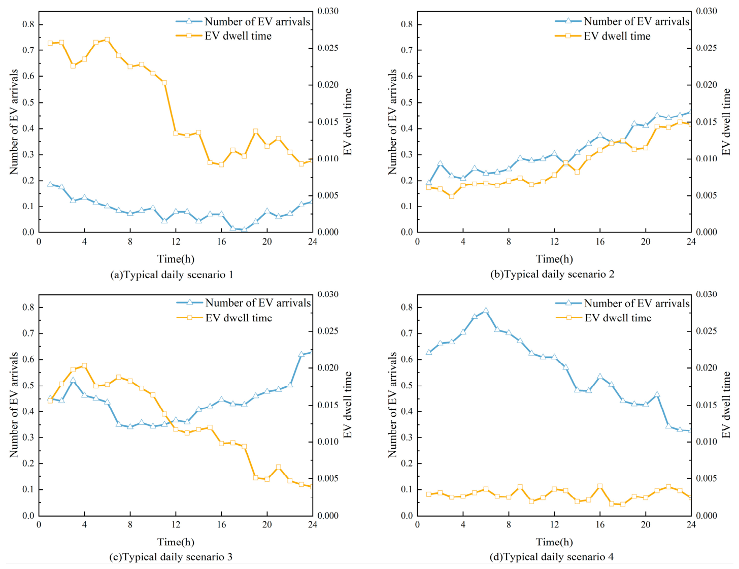
According to existing studies, the statistical characteristics of EV parking behavior at a specific destination can be jointly characterized by fitting the distribution curves of EV arrival quantity and EV dwell time. Figure 1 illustrates the distribution curves of EV arrival quantity and EV dwell time under different typical-day scenarios. Among them, the EV arrival quantity distribution curve is expressed in per-unit values, with the peak parking quantity at the destination taken as the base value. In the EV dwell time distribution curve, the probability corresponding to a given dwell time represents the proportion of EVs staying for that duration relative to the total number of arriving EVs.

In practical charging scenarios, EV users tend to prioritize charging facilities that can fulfill their charging requirements within the EV dwell time. When multiple types of charging facilities can satisfy the demand, users generally prefer lower-power options to reduce the additional battery degradation caused by high-power charging [22,23]. Due to variations in the state of charge upon arrival and the EV dwell time, EVs exhibit heterogeneous charging demands. Therefore, establishing a charging load model that reflects user demand characteristics can effectively describe the matching relationship between EV charging requirements and different types of charging facilities.

In this study, three types of charging facilities—SCFs, FCFs, and UCFs—are considered in distribution network planning. Specifically, SCFs are suitable for long-duration parking scenarios, FCFs can meet general charging demands, and UCFs are primarily used for short dwell times or urgent charging needs. By comparing the required charging energy of an EV with the energy that can be delivered by different charging facilities within the EV dwell time, the selected charging facility and its corresponding rated charging power can be determined. Accordingly, the rated charging power of the $k$-th EV can be expressed as

$$P_k=\{\begin{array}{c}{P}^{SCF} C_k(1-SO{C}_k)\le P^{SCF}{T}_k\hfill \\ P^{FCF} P^{SCF}{T}_k<C_k(1-SO{C}_k)\le P^{FCF}{T}_k\hfill \\ P^{UCF} C_k(1-SO{C}_k)>P^{FCF}{T}_k\hfill \end{array}$$

(1)

where $P^{SCF}$,$P^{FCF}$ and $P^{UCF}$ denote the rated charging power of slow, fast, and ultra-fast charging facilities, respectively; ${ C}_{k }$ represents the battery capacity of the $k$-th electric vehicle; ${ SOC}_{k }$ is the state of charge of the $k$-th EV upon arrival; and ${ T}_{k }$ denotes the EV dwell time of the $k$-th EV.

2.2. Charging Load Model of Stations with Multi-Type Electric Vehicle Charging Facilities

In practical operation, users’ selection of charging facilities is influenced not only by the EV state of charge (SOC) and the EV dwell time but also by the availability of idle charging facilities within the station. When the number of a certain type of charging facility is insufficient, some EVs may be forced to select alternative types, thereby altering the matching relationship between EVs and charging facilities and further affecting the actual charging load of the station.

To accurately characterize the charging load of the station, this paper constructs four scenarios based on the matching conditions between EV charging demand and available charging facilities and provides corresponding conditional descriptions. Moreover, these constraints are only applicable to nodes equipped with charging facilities.

Scenario 1: The number of all three types of charging facilities is sufficient to meet the charging demand of their corresponding EV categories. The condition for this scenario is given as follows:

$$\{\begin{array}{c}{N}_j^{SCF}\ge {\displaystyle \sum _{j=1}^{{\Phi }_{EV}}}{N}_j^{SCF,EV}\\ N_j^{FCF}\ge {\displaystyle \sum _{j=1}^{{\Phi }_{EV}}}{N}_j^{FCF,EV}\\ N_j^{UCF}\ge {\displaystyle \sum _{j=1}^{{\Phi }_{EV}}}{N}_j^{UCF,EV}\end{array}$$

(2)

At this point, the charging load of the EV charging station at node $j$, denoted by $P_j^{EV}$, can be expressed as

$$P_j^{EV}=P^{SCF}\sum _{j=1}^{{\Phi }_{EV}}{N}_j^{SCF,EV}+P^{FCF}\sum _{j=1}^{{\Phi }_{EV}}{N}_j^{FCF,EV}+P^{UCF}\sum _{j=1}^{{\Phi }_{EV}}{N}_j^{UCF,EV}$$

(3)

where ${ \Phi }_{EV }$ denotes the set of candidate nodes for new EV charging stations; ${ N}_j^{SCF }$, ${ N}_j^{FCF }$ and ${ N}_j^{UCF}$ represent the number of installed SCFs, FCFs and UCFs at node $j$, respectively; and $N_j^{SCF,EV}$, $N_j^{FCF,EV}$ and $N_j^{UCF,EV}$ denote the number of EVs using SCFs, FCFs, and UCFs at node $j$, respectively.

Scenario 2: The number of SCFs is insufficient; therefore, a portion of EVs originally assigned to SCFs must be reallocated to FCFs. The condition for this scenario is given as follows:

$$\{\begin{array}{c}{N}_j^{SCF}<{\displaystyle \sum _{j=1}^{{\Phi }_{EV}}}{N}_j^{SCF,EV}\hfill \\ N_j^{SCF}+N_j^{FCF}\ge {\displaystyle \sum _{j=1}^{{\Phi }_{EV}}}{N}_j^{SCF,EV}+N_j^{FCF,EV}\hfill \\ N_j^{UCF}\ge {\displaystyle \sum _{j=1}^{{\Phi }_{EV}}}{N}_j^{UCF,EV}\hfill \end{array}$$

(4)

At this point, the charging load of the EV charging station at node $j$, denoted by $P_j^{EV}$, can be expressed as

$$P_j^{EV}=P^{SCF}{N}_j^{SCF}+P^{FCF}(\sum _{j=1}^{{\Phi }_{EV}}{N}_j^{SCF,EV}-N_j^{SCF})+P^{FCF}\sum _{j=1}^{{\Phi }_{EV}}{N}_j^{FCF,EV}+P^{UCF}\sum _{j=1}^{{\Phi }_{EV}}{N}_j^{UCF,EV}$$

(5)

Scenario 3: The number of FCFs is insufficient; consequently, a portion of EVs originally assigned to FCFs must be reallocated to UCFs. The condition for this scenario is given as follows:

$$\{\begin{array}{c} N_j^{SCF}\ge {\displaystyle \sum _{j=1}^{{\Phi }_{EV}}}{N}_j^{SCF,EV}\hfill \\ N_j^{FCF}<{\displaystyle \sum _{j=1}^{{\Phi }_{EV}}}{N}_j^{FCF,EV}\hfill \\ { N}_j^{UCF}\ge {\displaystyle \sum _{j=1}^{{\Phi }_{EV}}}{N}_j^{UCF,EV}\hfill \end{array}$$

(6)

At this point, the charging load of the EV charging station at node $j$, denoted by $P_j^{EV}$, can be expressed as

$$P_j^{EV}=P^{SCF}\sum _{j=1}^{{\Phi }_{EV}}{N}_j^{SCF,EV}+P^{FCF}{N}_j^{FCF}+P^{UCF}(\sum _{j=1}^{{\Phi }_{EV}}{N}_j^{FCF,EV}-N_j^{FCF})+P^{UCF}\sum _{j=1}^{{\Phi }_{EV}}{N}_j^{UCF,EV}$$

(7)

Scenario 4: The numbers of both SCFs and FCFs are insufficient; therefore, a portion of EVs originally assigned to SCFs and FCFs must be connected to higher-power charging facilities. The condition for this scenario is given as follows:

$$\{\begin{array}{c} N_j^{SCF}<{\displaystyle \sum _{j=1}^{{\Phi }_{EV}}}{N}_j^{SCF,EV}\hfill \\ N_j^{SCF}+N_j^{FCF}<{\displaystyle \sum _{j=1}^{{\Phi }_{EV}}}{N}_j^{SCF,EV}+N_j^{FCF,EV}\hfill \\ { N}_j^{UCF}\ge {\displaystyle \sum _{j=1}^{{\Phi }_{EV}}}{N}_j^{UCF,EV}\hfill \end{array}$$

(8)

At this point, the charging load of the EV charging station at node $j$, denoted by $P_j^{EV}$, can be expressed as

$$P_j^{EV}=P^{SCF}{N}_j^{SCF}+{P^{FCF}N}_j^{FCF}+P^{UCF}\sum _{j=1}^{{\Phi }_{EV}}{N}_j^{UCF,EV}+P^{UCF}(\sum _{j=1}^{{\Phi }_{EV}}{N}_j^{SCF,EV}+\sum _{j=1}^{{\Phi }_{EV}}{N}_j^{FCF,EV}-N_j^{SCF}-N_j^{FCF})$$

(9)

3. Aumann–Shapley-Based Green Certificate-Tiered Carbon Trading Mechanism

3.1. Carbon Trading Model Based on the Aumann–Shapley Value Method

The carbon trading mechanism mainly consists of three components: carbon allowances, carbon emissions, and carbon trading prices. Among these, carbon allowances are typically allocated by governmental authorities based on industry-wide emission reduction targets. However, in a distribution network system with multiple participating entities, a single allocation approach is insufficient to reflect the respective contributions of each entity to emission reduction during system operation.

To address this issue, this paper employs the Aumann–Shapley value method to quantify the carbon emission responsibility of each participant in the distribution network and uses the results as the basis for carbon allowance allocation, thereby ensuring a fair distribution of carbon allowances.${ E}_{cea}$ denotes the carbon allowance allocated to participant $i$; it can be calculated using the Aumann–Shapley value method as follows:

$$Y_i=P_i^{DG}{\displaystyle \sum _{N=1}^M}{\displaystyle \frac{c(\frac{N}{M}{P}^{DG}+\Delta P_i^{DG})-c\left(\frac{N}{M}{P}^{DG}\right)}{M\Delta P_i^{DG}}}$$

(10)

$$E_{cea}=o{\displaystyle \frac{1}{T}}{\displaystyle \sum _{t=1}^T}{Y}_{i,t}$$

(11)

where ${ Y}_{i }$ denotes the carbon emission responsibility at node $i$ calculated using the Aumann–Shapley value method; $P_i^{DG}$ and ${∆P}_i^{DG}$ represent the injected power of distributed generation and its incremental variation at node $i$; $M$ and $N$ denote the number of segments and the segment index used in the Aumann–Shapley calculation; $c$ represents the carbon emission operator; $o$ is the carbon allowance factor.

Equation (10) represents the discretized form of the Aumann–Shapley continuous integral formulation. The integral interval $[0,1]$ is equally divided into $M$ subintervals, and the integral process is approximated using a discrete summation to calculate the marginal carbon responsibility. $M$ denotes the number of discretization segments, which affects both calculation accuracy and computational efficiency. When $M$ is too small, the discretization error of the integral is relatively large; conversely, an excessively large $M$ increases the computational scale and solution time of the model. Considering both model accuracy and computational efficiency, multiple tests were conducted in this study, and $M=100$ was selected as the discretization segment number. When $M\ge 100$, the variation in the carbon allowance allocation results for each participant is less than 0.5%, indicating that the integral results have essentially converged. Therefore, the proposed setting can ensure allocation fairness while maintaining favorable computational efficiency and scalability, making it more suitable for bi-level distribution network expansion planning problems.

The carbon emissions of the distribution network can be expressed as the product of electricity consumption and the corresponding carbon emission intensity. Considering that carbon emissions in distribution networks mainly originate from electricity purchased from the upstream grid [14], this paper adopts the carbon emission flow theory and introduces a dynamic carbon emission factor to calculate system emissions, as expressed in (12).

$$\{\begin{array}{c} E_{carbon}={\tau }_{co2}{P}^{GRID}\\ E_{ct}=E_{carbon}-E_{cea}\end{array}$$

(12)

where ${ E}_{carbon }$ denotes the indirect carbon emissions of the distribution network; ${ P}^{GRID }$ represents the electricity purchased from the upstream grid; ${ \tau }_{co2 }$ is the dynamic carbon emission factor; ${ E}_{ct }$ denotes the carbon emissions of the distribution network under the carbon trading mechanism; and $k$ represents the interval length of different carbon allowance segments.

3.2. Green Certificate Trading

Green certificate trading requires the energy side to fulfill renewable energy consumption obligations. By converting the consumed distributed renewable energy into green certificates, the consumption behavior of distributed energy can be quantified. The number of green certificates obtained from distributed generation can be calculated as

$$G_{green}={\lambda }_g\sum _{s\in {\Omega }_s}{\rho }_s\sum _{t=1}^{24}(\sum _{i\in {\Phi }_{WTG}}{P}_{i,t,s}^{WTG}+\sum _{i\in {\Phi }_{PVG}}{P}_{i,t,s}^{PVG})$$

(13)

where ${ G}_{green }$ denotes the number of green certificates converted from renewable energy generation, and ${ \lambda }_{g }$ is the conversion coefficient from renewable energy generation to green certificates.

3.3. Aumann–Shapley-Based Green Certificate-Tiered Carbon Trading Mechanism

In this paper, the number of green certificates obtained by the system is equivalently converted into carbon allowances, thereby incorporating green certificate trading into the carbon emission constraint framework. Meanwhile, to strengthen the regulation of system carbon emissions, a tiered carbon trading scheme is adopted, in which different price intervals are defined according to emission levels. Specifically, higher carbon emissions correspond to higher carbon prices, thereby imposing economic penalties on high-emission behaviors [2]. The detailed formulation is given as follows:

$$E_{co2}=E_{ct}-{\xi }_g{G}_{green}$$

(14)

$$C^{CO2}=\{\begin{array}{c} \sigma E_{co2} \hspace{0.33em}0<E_{co2}\le l\hfill \\ \sigma l+\sigma \left(1+\chi \right)\left(E_{co2}-l\right) l<E_{co2}\le 2l\hfill \\ \sigma (2+\chi )l+\sigma \left(1+2\chi \right)\left(E_{co2}-2l\right) E_{co2}>2l\hfill \end{array}$$

(15)

where ${ E}_{co2 }$ denotes the carbon emissions participating in the integrated green certificate-tiered carbon trading; ${ \xi }_{g }$ is the green certificate conversion factor; ${ C}^{CO2 }$ represents the carbon emission cost; $\sigma$ denotes the base carbon price; $l$ is the interval length of carbon emission segments; and $\chi$ represents the growth rate of carbon trading cost.

4. Low-Carbon Distribution Network Expansion Planning Model

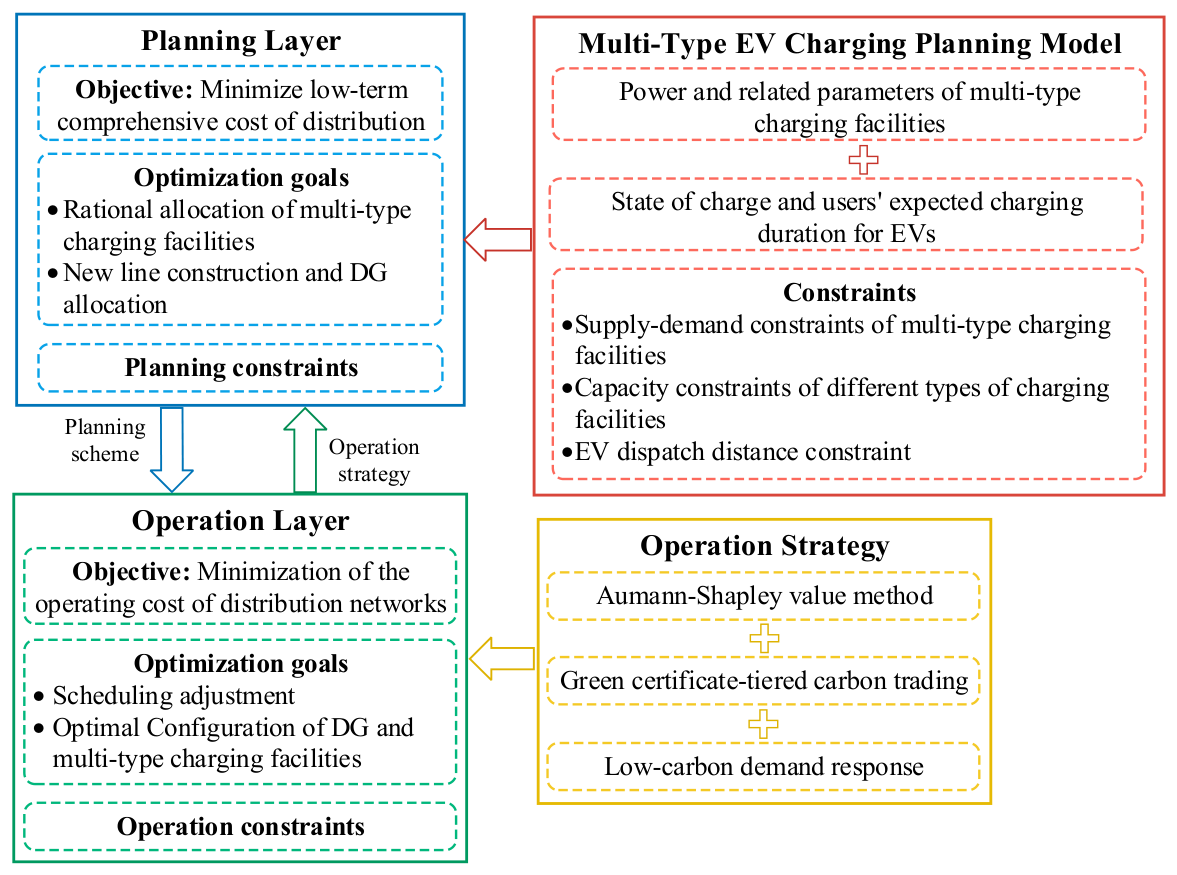
Distribution network expansion planning involves two distinct layers of optimization: long-term planning decisions and short-term operational scheduling, which differ in time scale and decision objectives. To capture the impact of planning schemes on system operational states and achieve coordinated optimization between planning and operation, the low-carbon distribution network expansion planning model in this study is divided into a planning layer and an operation layer. The overall framework of the bi-level distribution network expansion planning model is illustrated in Figure 2.

In the planning layer, the objective is to minimize the annual total cost of the distribution network. The multi-type EV charging station model is integrated into this layer, enabling the coordinated siting and capacity allocation of distribution lines, WTG, PVG, ESS and EV charging stations. In the operation layer, given a planning scheme, the objective is to minimize the operational cost of the distribution network. The improved integrated green certificate-tiered carbon trading and low-carbon demand response model is employed to optimize system operation, ensuring that the planning scheme achieves both economic efficiency and low-carbon performance.

4.1. Objective Function

4.1.1. Objective Function of the Planning Layer

The objective function of the distribution network planning layer aims to minimize the annual total cost over the planning horizon, which consists of the annualized planning investment cost and the system operating cost, i.e.,

$$\mathrm{m}\mathrm{i}\mathrm{n} C^{TOTAL}=C^{INV}+C^{OPE}$$

(16)

The planning investment cost includes the investment costs of EV charging stations, distribution lines, WTG, PVG, and ESS, which can be expressed as

$$C^{INV}=C^{EV}+C^{LINE}+C^{WTG}+C^{PVG}+C^{ESS}$$

(17)

$${\gamma }^e=d(1+d{)}^{y^e}/[(1+d{)}^{y^e}-1]$$

(18)

$$\{\begin{array}{c} C^{EV}={\gamma }^e{\displaystyle \sum _{i\in {\Phi }_{EV}}}{x}_i^{EV}\left(c^{\mathit{SCF}}{N}_i^{SCF}+c^{\mathit{FCF}}{N}_i^{FCF}+c^{\mathit{UCF}}{N}_i^{UCF}\right)\hfill \\ C^{LINE}={\gamma }^e{\displaystyle \sum _{i\in {\Phi }_{LINE}}}{c}^{LINE}{x}_i^{LINE}{L}_i\hfill \\ C^{WTG}={\gamma }^e{\displaystyle \sum _{i\in {\Phi }_{WTG}}}{c}^{WTG}{x}_i^{WTG}{S}^{WTG}\hfill \\ C^{PVG}={\gamma }^e{\displaystyle \sum _{i\in {\Phi }_{PVG}}}{c}^{PVG}{x}_i^{PVG}{S}^{PVG}\hfill \\ C^{ESS}={\gamma }^e{\displaystyle \sum _{i\in {\Phi }_{ESS}}}{c}^{ESS}{x}_i^{ESS}{S}^{ESS}\hfill \end{array}$$

(19)

where ${ \gamma }^{e }$ denotes the annualization factor of component $e$; $d$ is the discount rate; and ${ y}^{e }$ represents the service lifetime of component $e$. ${\Phi }_{LINE }$, ${\Phi }_{WTG }$, ${\Phi }_{PVG }$ and ${\Phi }_{ESS }$ denote the sets of candidate nodes for candidate new lines, candidate nodes for WTG, PVG and ESS, respectively. ${ c}^{SCF },{ c}^{FCF }$ and ${ c}^{UCF }$ represent the unit investment costs of SCFs, FCFs, and UCFs, respectively. ${ c}^{LINE }$ is the unit construction cost per unit length of distribution lines. ${ c}^{WTG }$, ${ c}^{PVG }$ and ${ c}^{ESS }$ denote the unit capacity investment costs of WTG, PVG and ESS, respectively. ${ x}_i^{EV }$, ${ x}_i^{LINE }$, ${ x}_i^{WTG }$, ${ x}_i^{PVG }$ and ${ x}_i^{ESS }$ are the decision variables for charging station construction, line expansion, and the installation of WTG, PVG and ESS, respectively. ${ L}_{i }$ represents the length of candidate lines. ${ S}^{WTG }$, ${ S}^{WTG }$ and ${ S}^{WTG }$ denote the installed capacities of WTG, PVG and ESS, respectively.

4.1.2. Objective Function of the Operation Layer

The operation layer of the distribution network aims to minimize the annual operating cost of the system. The total annual operating cost consists of equipment operation cost, electricity purchasing cost from the upstream grid, network loss cost, wind and solar curtailment cost, carbon emission cost, and demand response cost, i.e.,

$$\min C^{OPE}=C^{OM}+C^{BUY}+C^{LOSS}+C^Q+C^{CO2}+C^{DR}$$

(20)

$$\{\begin{array}{l}{C}^{OM}={\displaystyle \sum _{i\in {\Phi }_{ESS}}}{x}_i^{EV}(c_{\mathit{SCF}}^{\mathit{OM}}{N}_i^{SCF}+c_{\mathit{FCF}}^{\mathit{OM}}{N}_i^{FCF}+c_{\mathit{UCF}}^{\mathit{OM}}{N}_i^{UCF})+\hfill \\ {\displaystyle \sum _{i\in {\Phi }_{ESS}}}{c}_{ESS}^{OM}{E}_i^{ESS}+365{\displaystyle \sum _{s\in {\Omega }_s}}{\rho }_s{\displaystyle \sum _{t=1}^{24}}({\displaystyle \sum _{i\in {\Phi }_{WTG}}}{c}_{WTG}^{OM}{P}_{i,t,s}^{WTG}+{\displaystyle \sum _{i\in {\Phi }_{PVG}}}{c}_{PVG}^{OM}{P}_{i,t,s}^{PVG})\hfill \\ C^{BUY}=365{\displaystyle \sum _{s\in {\Omega }_s}}{\rho }_s{\displaystyle \sum _{t=1}^{24}}{c}^{BUY}{P}_{t,s}^{GRID}\\ C^{LOSS}=365{\displaystyle \sum _{s\in {\Omega }_s}}{\rho }_s{\displaystyle \sum _{t=1}^{24}}{\displaystyle \sum _{ij\in {\Omega }_{line}}}{c}^{LOSS}{R}_{ij}{I}_{ij,t,s}^2\\ C^Q=365{\displaystyle \sum _{s\in {\Omega }_s}}{\rho }_s{\displaystyle \sum _{t=1}^{24}}({\displaystyle \sum _{i\in {\Phi }_{WTG}}}{c}_{WTG}^Q{P}_{i,t,s}^{WTG,Q}+{\displaystyle \sum _{i\in {\Phi }_{PVG}}}{c}_{PVG}^Q{P}_{i,t,s}^{PVG,Q})\\ C^{DR}=365{\displaystyle \sum _{s\in {\Omega }_s}}{\rho }_s{\displaystyle \sum _{t=1}^{24}}{\displaystyle \sum _{i\in {\Phi }_{IDR}}}(c_{i,t}^{IDR}\left|\Delta P_{i,t}^{IDR}\right|)+365{\displaystyle \sum _{s\in {\Omega }_s}}{\rho }_s{\displaystyle \sum _{t=1}^{24}}{\displaystyle \sum _{i\in {\Phi }_{PDR}}}(c_{i,t}^{PDR}\left|P_{i,t}^{ORI}-P_{i,t}^{PDR}\right|)\end{array}$$

(21)

where ${\Omega }_s$ and ${\Omega }_{line}$ denote the set of time periods in a typical daily scenario and the set of distribution network lines, respectively; $s$ represents the current typical daily scenario; and ${\rho }_s$ denotes the probability of scenario $s$. $c_{SCF}^{OM}$, $c_{FCF}^{OM}$, $c_{UCF}^{OM}$ and $c_{ESS}^{OM}$ represent the annual operation and maintenance costs per unit installed capacity of SCFs, FCFs, UCFs, and ESS, respectively. $c_{WTG}^{OM}$ and $c_{PVG}^{OM}$ denote the operating costs per unit energy of WTG and PVG, respectively. $E_i^{ESS}$ is the decision variable representing the capacity of ESS. $P_{i,t,s}^{WTG}$ and $P_{i,t,s}^{PVG}$ denote the active power outputs of WTG and PVG respectively. $c^{BUY}$ represents the electricity purchasing price from the upstream grid. $c^{LOSS}$ denotes the unit cost of network losses. $R_{ij}$ is the line impedance of branch $l$, and $I_{ij,t,s}^2$ represents the squared current of branch $l$. $c_{WTG }^Q$ and $c_{PVG }^Q$ denote the penalty costs for wind and photovoltaic curtailment per unit power, respectively; $P_{i,t,s}^{WTG,Q}$ and $P_{i,t,s}^{PVG,Q}$ represent the curtailed wind and photovoltaic power, respectively.

4.2. Constraints

4.2.1. Constraints of the Planning Layer

• Capacity constraints on different types of charging facilities in EV charging stations:

$$\{\begin{array}{l} N_j^{UCF}\ge {\displaystyle \sum _{j=1}^{{\Phi }_{EV}}}{N}_j^{SCF,EV} \\ N_j^{FCF}+N_j^{UCF}\ge {\displaystyle \sum _{j=1}^{{\Phi }_{EV}}}{N}_j^{FCF,EV}+N_j^{UCF,EV}\\ N_j^{SCF}+N_j^{FCF}+N_j^{UCF}\ge {\displaystyle \sum _{j=1}^{{\Phi }_{EV}}}{N}_j^{SCF,EV}+N_j^{FCF,EV}+N_j^{UCF,EV}\end{array}$$

(22)

2.

Constraints on distributed generation (DG) and line expansion:

$$\{\begin{array}{l} x_j^{LINE}\le 1\hspace{1em}\forall j\in {\Phi }_{LINE}\\ 0\le {\displaystyle \sum _{j\in {\Phi }_{WTG}}}{x}_j^{WTG}\le N_{WTG,MAX}\\ 0\le {\displaystyle \sum _{j\in {\Phi }_{PVG}}}{x}_j^{PVG}\le N_{PVG,MAX}\\ 0\le {\displaystyle \sum _{j\in {\Phi }_{ESS}}}{x}_j^{ESS}\le N_{ESS,MAX}\end{array}$$

(23)

where ${ N}_{WTG,MAX }$, ${ N}_{WTG,MAX}$ and $N_{WTG,MAX}$ denote the maximum number of WTG, PVG, and ESS that can be installed at node $j$, respectively.

4.2.2. Constraints of the Operation Layer

• Operational constraints of EV charging stations:

$$\{\begin{array}{c} N_{ij}^{SCF}=0,\forall (i,j)\in \left\{(i,j)\left|d\right(i,j)>d_{max}\right\}\\ N_{ij}^{FCF}=0,\forall (i,j)\in \left\{(i,j)\left|d\right(i,j)>d_{max}\right\}\\ N_{ij}^{UCF}=0,\forall (i,j)\in \left\{(i,j)\left|d\right(i,j)>d_{max}\right\}\end{array}$$

(24)

where ${ N}_{ij}^{SCF }$, ${ N}_{ij}^{FCF }$ and ${ N}_{ij}^{UCF }$ denote the number of EVs traveling from node $i$ to node $j$ and using SCFs, FCFs, and UCFs, respectively; $d\left(i,j\right)$ represents the distance between node $i$ and node $j$; $d_{max}$ denotes the maximum acceptable dispatch distance for EV users to reach the destination charging station.

2.

Operational constraints of photovoltaic and wind power generation:

$$\{\begin{array}{l} 0\le P_{i,t,s}^{WTG}\le P_{i,s,max}^{WTG}\\ 0\le P_{i,t,s}^{PVG}\le P_{i,s,max}^{PVG}\\ Q_{i,t,s}^{DG}=P_{i,t,s}^{DG}\mathit{tan}\phi \\ P_{i,t,s}^{WTG,Q}=P_{i,s,max}^{WTG}-P_{i,t,s}^{WTG}\\ P_{i,t,s}^{PVG,Q}=P_{i,s,max}^{PVG}-P_{i,t,s}^{PVG}\end{array}$$

(25)

where ${ P}_{i,s,max }^{WTG }$ and ${ P}_{i,s,max }^{PVG }$ denote the maximum active power outputs of WTGs and PVGs, respectively; ${ Q}_{i,t,s }^{DG}$ and ${ P}_{i,t,s }^{DG}$ represent the reactive and active power injections of distributed generation, respectively; and $\phi$ denotes the power factor angle of distributed generation.

3.

Charging and discharging constraints of energy storage systems:

$$\{\begin{array}{l} z_{i,t,s}^{ch}+z_{i,t,s}^{dis}\le 1\\ 0\le P_{i,t,s}^{ch}\le z_{i,t,s}^{ch}{P}_{i,s}^{ch,max}\\ 0\le P_{i,t,s}^{dis}\le z_{i,t,s}^{dis}{P}_{i,s}^{dis,max}\\ E_{i,t+\Delta t,s}^{ESS}=E_{i,t,s}^{ESS}+P_{i,t,s}^{ch}\Delta t\times {\eta }_{ch}-{\displaystyle \frac{P_{i,t,s}^{dis}\Delta t}{{\eta }_{dis}}}\\ E_{i,s}^{ESS,min}\le E_{i,t,s}^{ESS}\le E_{i,s}^{ESS,max}\\ { E}_{i,0,s}^{ESS}=E_{i,24,s}^{ESS}\end{array}$$

(26)

where ${ z}_{i,t,s }^{ch}$ and ${ z}_{i,t,s }^{dis}$ denote the charging and discharging state variables of the ESS, respectively; ${ P}_{i,t,s }^{ch}$ and ${ P}_{i,t,s }^{dis}$ represent the charging and discharging power, respectively; ${ P}_{i,s }^{ch,max }$ and ${ P}_{i,s }^{dis,max }$ denote the maximum charging and discharging power of the ESS; ${ E}_{i,t,s }^{ESS}$ represents the remaining energy of the ESS; ${ E}_{i,s }^{ESS,min}$ and ${ E}_{i,s }^{ESS,max}$ denote the minimum and maximum energy capacity limits of the ESS, respectively.

4.

Node voltage and branch current constraints:

$$\{\begin{array}{l} V_{min}^2\le V_{i,t,s}^2\le V_{max}^2\\ 0\le I_{ij,t,s}^2\le I_{max}^2\end{array}$$

(27)

where ${ V}_{min }$ and ${ V}_{max }$ denote the minimum and maximum voltage limits of nodes, respectively; ${ V}_{i,t,s }^2$ represents the squared voltage magnitude at node $i$; and ${ I}_{max }$ denotes the maximum allowable current of branches.

5.

DistFlow power flow constraints:

$$\{\begin{array}{l} {\displaystyle \sum _{j\in {\kappa }_i}}{P}_{ij,t,s}-{\displaystyle \sum _{k\in {\nu }_i}}(P_{ki,t,s}-I_{ki,t,s}^2{R}_{ki})=P_{i,t,s}^{in}\\ {\displaystyle \sum _{j\in {\kappa }_i}}{Q}_{ij,t,s}-{\displaystyle \sum _{k\in {\nu }_i}}(Q_{ki,t,s}-I_{ki,t,s}^2{X}_{ki})=Q_{i,t,s}^{in}\\ (V_{i,t,s}^2-V_{j,t,s}^2)-2(P_{ij,t,s}{R}_{ij}+X_{ij}{Q}_{ij,t,s})+I_{ij,t,s}^2(R_{ij}^2+X_{ij}^2)\ge -M(1-x_j^{LINE})\\ (V_{i,t,s}^2-V_{j,t,s}^2)-2(P_{ij,t,s}{R}_{ij}+X_{ij}{Q}_{ij,t,s})+I_{ij,t,s}^2(R_{ij}^2+X_{ij}^2)\le M(1-x_j^{LINE})\\ I_{ij,t,s}^2{V}_{ij,t,s}^2-P_{ij,t,s}^2-Q_{ij,t,s}^2=0\\ P_{i,t,s}^{in}=P_{i,t,s}^{WTG}+P_{i,t,s}^{PVG}+P_{i,t,s}^{ESS}+P_{i,t,s}^{EV}-P_{i,t,s}^L+P_{i,t,s}^{GRID}\\ Q_{i,t,s}^{in}=Q_{i,t,s}^{WTG}+Q_{i,t,s}^{PVG}+Q_{i,t,s}^{ESS}+Q_{i,t,s}^{EV}-Q_{i,t,s}^L+Q_{i,t,s}^{GRID}\end{array}$$

(28)

where ${\kappa }_i$ and ${\nu }_i$ denote the sets of lines with node $i$ as the receiving end and sending end, respectively; $P_{ij,t,s}$ and $Q_{ij,t,s}$ represent the active and reactive power flows on branch $ij$, respectively; $X_{ki}$ denotes the reactance of branch $ki$; $P_{i,t,s }^{in}$ and $Q_{i,t,s }^{in}$ represent the active and reactive power injections at node $i$, respectively; $M$ is a sufficiently large positive constant; $P_{i,t,s }^{EV}$ and $P_{i,t,s }^L$ denote the active power of EV charging stations and the load at node $i$, respectively; $Q_{i,t,s }^{WTG}$, $Q_{i,t,s }^{PVG}$, $Q_{i,t,s }^{ESS}$, $Q_{i,t,s }^{EV}$, $Q_{i,t,s }^L$ and $Q_{i,t,s }^{GRID}$ denote the reactive power of WTG, PVG, ESS, EV charging stations, loads at node $i$, and the upstream grid, respectively.

6.

Demand response (DR) constraints:

$$\{\begin{array}{l} P_{i,t}^{ORI}-P_{i,t}^{PDR}={\zeta }_{PDR}(c_{i,t}^{PDR}-c_{i,t}^{ORI})\\ {\displaystyle \sum _{i=1}^{BUS}}{\displaystyle \sum _{t=1}^T}{P}_{i,t}^{PDR}={\displaystyle \sum _{i=1}^{BUS}}{\displaystyle \sum _{t=1}^T}{P}_{i,t}^{ORI}\\ c_{i,t}^{PDR,min}\le c_{i,t}^{PDR}\le c_{i,t}^{PDR,max}\end{array}$$

(29)

where ${ P}_{i,t }^{ORI }$ and ${ P}_{i,t }^{PDR }$ denote the load demand before and after price-based demand response, respectively; ${ \zeta }_{PDR }$ is the price elasticity coefficient; ${ c}_{i,t }^{ORI }$ and ${ c}_{i,t }^{PDR }$ represent the electricity prices before and after demand response, respectively; $BUS$ denotes the total number of nodes in the distribution network system; ${ c}_{i,t }^{PDR,min }$ and ${ c}_{i,t }^{PDR,max }$ denote the minimum and maximum electricity prices after demand response, respectively.

Incentive-based demand response is primarily implemented in the form of load reduction. Considering the response characteristics of reducible loads, the amount of load reduction should satisfy the following constraints:

$$\Delta P_{i,min}^{IDR}\le \Delta P_{i,t}^{IDR}\le \Delta P_{i,max}^{IDR}$$

(30)

where ${ ∆P}_{i,t }^{IDR }$ denotes the load reduction, ${ ∆P}_{i,min }^{IDR }$ and ${ ∆P}_{i,max }^{IDR }$ represent the minimum and maximum allowable load reduction, respectively.

7.

Radial structure and connectivity constraints:

During the expansion planning of distribution networks, the formation of looped structures should be avoided. The design principle follows a closed-loop design with open-loop operation, ensuring compliance with radial topology constraints. Under the connectivity requirement, a basic constraint is that the number of lines in the final planning scheme should be one less than the number of nodes. In addition, to guarantee the connectivity of all nodes in the planned network, a connectivity check of the resulting distribution topology is required [24,25,26].

$$n=m+1$$

(31)

where $n$ and $m$ denote the total number of nodes and the total number of lines in the planned distribution network, respectively.

4.3. Model Reformulation and Solution

4.3.1. Model Reformulation

In the distribution network planning model with multi-type charging facilities, a large-scale mixed-integer nonlinear programming (MINLP) problem constrained by scenario-dependent conditions is involved. To improve tractability, the conditional scenario constraints in (2)–(9) are transformed into deterministic constraints through relaxation.

First, the original conditional constraints are reformulated in a unified manner. Using an equivalent relaxation approach, equality constraints are transformed into a unified set of inequality constraints. Equations (3), (5), (7), and (9) can be collectively expressed as

$$P_j^{EV}=F\left(x\right)$$

(32)

where $F\left(x\right)$ denotes the function formed by the right-hand sides of the above equations. The model is then relaxed such that the equality constraints are replaced by inequality constraints. Assume that the optimal solution is obtained at a certain point, and the charging station load at this point satisfies the EV charging demand. Then, within a certain interval, there must exist a value that satisfies the original equality constraint.

As more EVs enter the charging station, the charging load increases monotonically. Since the corresponding function is monotonically increasing, the relaxed model would admit a better solution, which contradicts the assumption of optimality. Therefore, the assumption does not hold. Consequently, the relaxed model preserves the validity of the original equality constraints at the optimal solution, enabling unified modeling of charging load constraints under different scenarios while improving model solvability.

Moreover, since the system operating cost, electricity purchasing cost, and network loss cost in the objective function are all monotonically increasing with respect to the associated decision variables, the optimization process tends to minimize the relaxed variables while satisfying system operational constraints. If a relaxed inequality constraint is not active at the optimum, the objective function value can be further reduced by decreasing the corresponding variable, which contradicts the optimality condition. Therefore, at the optimal solution, the relaxed inequality constraints naturally converge to the original equality constraints, indicating that the proposed relaxation is exact.

By reformulating (2)–(9), the charging station load constraints under the four scenarios can be expressed as follows:

$$\{\begin{array}{l} s.t. Equation \left(2\right)\hspace{0.33em}\hspace{0.33em}\hspace{0.33em}\\ P_j^{EV}\ge P^{SCF}{\displaystyle \sum _{j=1}^{{\Phi }_{EV}}}{N}_j^{SCF,EV}+P^{FCF}{\displaystyle \sum _{j=1}^{{\Phi }_{EV}}}{N}_j^{FCF,EV}+P^{UCF}{\displaystyle \sum _{j=1}^{{\Phi }_{EV}}}{N}_j^{UCF,EV}\\ s.t. Equation \left(4\right)\\ P_j^{EV}\ge P^{SCF}{N}_j^{SCF}+P^{FCF}({\displaystyle \sum _{j=1}^{{\Phi }_{EV}}}{N}_j^{SCF,EV}-N_j^{SCF})+P^{FCF}{\displaystyle \sum _{j=1}^{{\Phi }_{EV}}}{N}_j^{FCF,EV}+P^{UCF}{\displaystyle \sum _{j=1}^{{\Phi }_{EV}}}{N}_j^{UCF,EV}\\ s.t. Equation \left(6\right)\\ P_j^{EV}\ge P^{SCF}{\displaystyle \sum _{j=1}^{{\Phi }_{EV}}}{N}_j^{SCF,EV}+P^{FCF}{N}_j^{FCF}+P^{UCF}({\displaystyle \sum _{j=1}^{{\Phi }_{EV}}}{N}_j^{FCF,EV}-N_j^{FCF})+P^{UCF}{\displaystyle \sum _{j=1}^{{\Phi }_{EV}}}{N}_j^{UCF,EV}\\ s.t. Equation \left(8\right)\\ P_j^{EV}\ge P^{SCF}{N}_j^{SCF}+P^{FCF}{N}_j^{FCF}+P^{UCF}{\displaystyle \sum _{j=1}^{{\Phi }_{EV}}}{N}_j^{UCF,EV}+P^{UCF}({\displaystyle \sum _{j=1}^{{\Phi }_{EV}}}{N}_j^{SCF,EV}+{\displaystyle \sum _{j=1}^{{\Phi }_{EV}}}{N}_j^{FCF,EV}-N_j^{SCF}-N_j^{FCF})\end{array}$$

(33)

Since the DistFlow power flow model of the distribution network contains multiplicative relationships among branch power, current, and node voltage, namely,

$$I_{ij,t,s}^2{V}_{ij,t,s}^2-P_{ij,t,s}^2-Q_{ij,t,s}^2=0$$

(34)

The above constraint is a typical nonconvex constraint, which makes the original model a mixed-integer nonlinear programming (MINLP) problem and difficult to solve efficiently using commercial solvers directly. To reduce the computational complexity, auxiliary variables are introduced as $U_{i,t,s}^{sqr}=V_{i,t,s }^2$ and $I_{ij,t,s}^{sqr}=I_{ij,t,s }^2$, representing the squared node voltage and squared branch current, respectively. Accordingly, the original nonconvex constraint can be transformed into

$$P_{ij,t,s}^2+Q_{ij,t,s}^2\le U_{i,t,s}^{sqr}{I}_{ij,t,s}^{sqr}$$

(35)

Furthermore, by applying the second-order cone relaxation (SOCR) method, the above constraint can be reformulated into a standard second-order cone form:

$$\Vert \begin{array}{c}2P_{ij,t,s}\\ 2Q_{ij,t,s}\\ U_{i,t,s}^{sqr}-I_{ij,t,s}^{sqr}\end{array}\Vert \le U_{i,t,s}^{sqr}+I_{ij,t,s}^{sqr}$$

(36)

Through the above SOCR treatment, the original MINLP model is transformed into a mixed-integer second-order cone programming (MISOCP) model. For radial distribution network structures, when node loads are positive, voltage upper and lower bounds are reasonably specified, and line impedance parameters satisfy practical engineering ranges, the SOCR generally exhibits good exactness properties. Under these conditions, the optimal solution of the relaxed problem can satisfy the original nonconvex power flow equations, thereby ensuring the physical feasibility and engineering rationality of the obtained results.

Through the above transformation, the solution difficulty of the original model can be significantly reduced while maintaining high solution accuracy. The resulting model can be efficiently solved using the Gurobi optimizer, with an optimality gap of 0.01% and an average computation time of approximately 40 s. During the solution process, the objective function gradually converges.

4.3.2. Model Solution

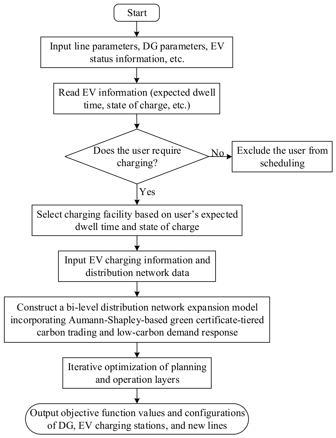
As shown in Figure 3, a bi-level expansion planning solution framework for low-carbon distribution networks considering multi-type charging facilities is proposed.

First, the parameters of the distribution network, candidate new lines, DG, and EVs are input, and key information such as the EV dwell time and initial state of charge of EV is obtained. By identifying users’ charging requirements and incorporating their dwell characteristics, appropriate matching among different types of charging facilities is achieved, enabling an accurate representation of heterogeneous charging behaviors. On this basis, a green certificate-tiered carbon trading mechanism based on the Aumann–Shapley value method and a low-carbon demand response model is established, forming a bi-level optimization framework. Through iterative coordination between the planning layer and the operation layer, coordinated optimization is realized.

Finally, the optimal results are obtained, including the configuration of distributed generation, the layout of charging facilities, and the expansion plan of distribution lines. The proposed method not only provides a refined characterization of multi-type charging demand but also introduces a fair and efficient carbon allowance allocation mechanism, thereby improving both the economic performance and low-carbon characteristics of distribution network planning.

5. Case Study Analysis

5.1. Case Study Setup

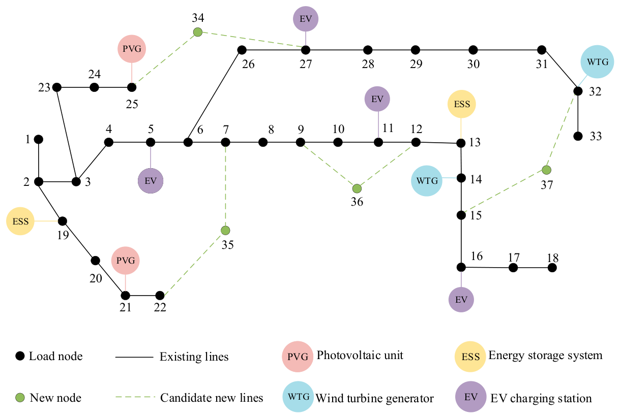
The improved IEEE 33-node distribution network system is adopted in this paper to verify the established model, as shown in Figure 4. The relevant parameters of the three different types of EV charging piles included in the EV charging station are presented in

Table 2. Parameters of multi-type electric vehicle charging facilities.

Relevant Parameters	SCF	FCF	UCF
Rated charging power (kW)	15	60	300
Investment cost (CNY/unit)	35,000	70,000	140,000
Operation and maintenance cost (CNY/unit/year)	3500	7000	14,000

. The model constructed in this paper can be mathematically modeled on the MATLAB R2019b simulation platform using the YALMIP toolbox and solved linearly by calling Gurobi 11.0.0.

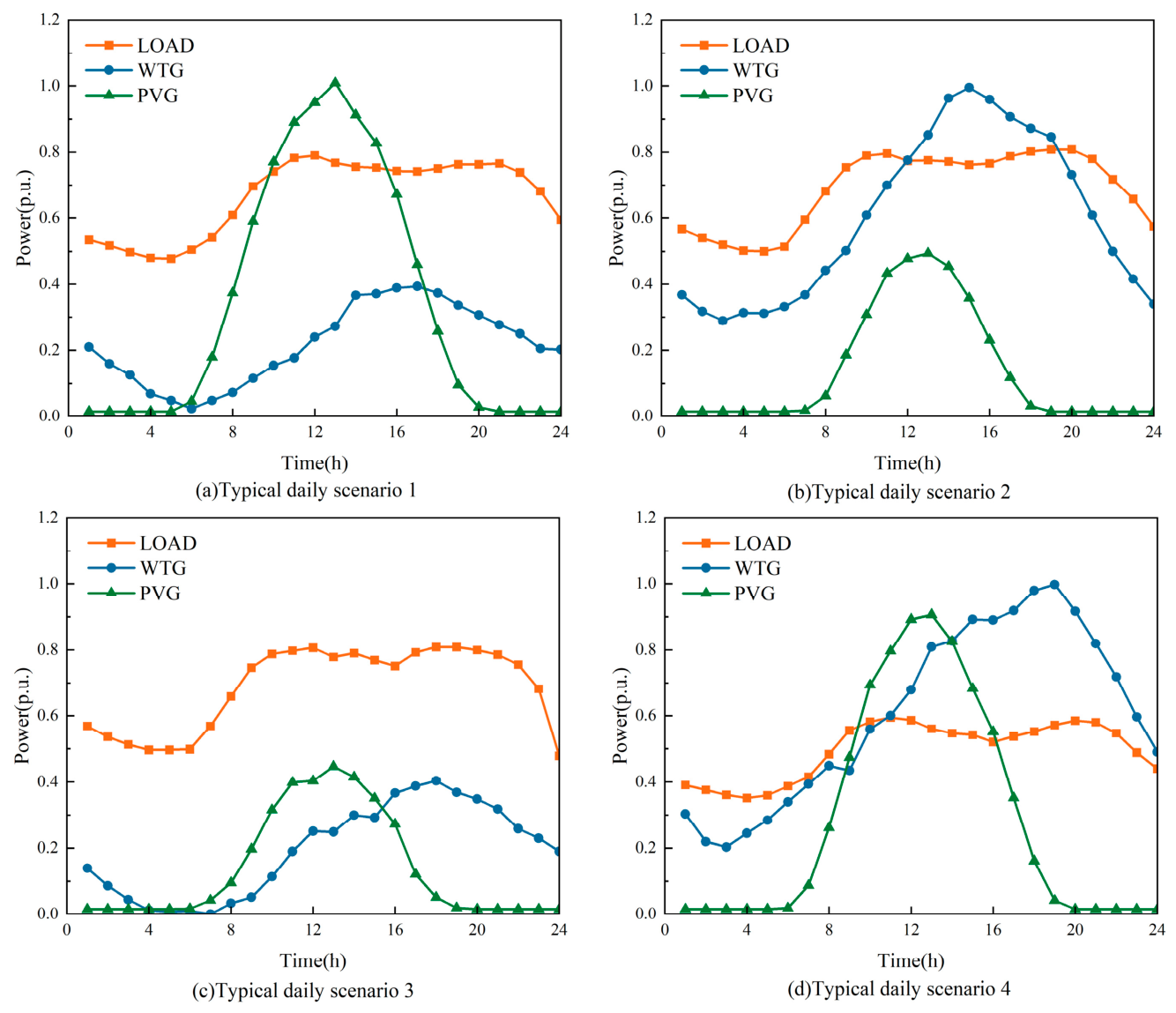
The load, wind power and photovoltaic output under each typical day scenario are shown in Figure 5, referring to the results of reference [27] for the typical day scenarios of wind and photovoltaic power. The probabilities of the four typical day scenarios are 0.221, 0.255, 0.379 and 0.145 respectively.

The maximum number of installed WTG, PVG, and ESS in the system is limited to five units each. The candidate nodes for WTG installation are nodes 14 and 32. The unit capacity investment cost of WTG is 8000 CNY/kW, and the operation and maintenance (O&M) cost per unit energy is 0.35 CNY/kWh, with a rated capacity of 250 kW per unit. The candidate nodes for PVG installation are nodes 21 and 25. The unit capacity investment cost is 9000 CNY/kW, and the O&M cost per unit energy is 0.28 CNY/kWh, with a rated capacity of 200 kW per unit. The penalty cost for wind and PV curtailment is 0.7 CNY/kWh. The candidate nodes for ESS installation are nodes 13 and 19. The unit capacity investment cost is 2500 CNY/kW, and the O&M cost per unit energy is 0.3 CNY/kWh, with a rated capacity of 200 kW per unit. The charging and discharging efficiency is 0.95, and the state-of-charge limits are set to 0.1 and 0.9, respectively. The unit cost of network losses is 0.6 CNY/kWh. The unit cost of load reduction is 0.8 CNY/kWh, and the compensation cost for load shifting is 0.5 CNY/kWh. The base carbon trading price is 750 CNY/t, the interval length of carbon emissions is 30 t, and the growth rate of carbon trading cost is 0.4. The conversion coefficient from renewable energy generation to green certificates is 1 certificate/MW, and the green certificate conversion factor is 0.09 t/certificate. The peak number of EVs at each node is obtained from [22]. The total number of electric vehicles considered in the system is approximately 4000. The data for candidate new lines and the dynamic carbon emission intensity of electricity purchased from the upstream grid are adopted from [13,14]. The battery capacity of EVs is set to 100 kWh, and the SOC of the EV upon arrival at the charging station is assumed to follow a uniform distribution within the interval [0, 1]. The service life of all equipment is assumed to be 15 years, and the discount rate is set to 5%.

5.2. Planning Results and Analysis Considering Multi-Type Charging Facilities

In this study, four charging station planning schemes are designed to analyze the impact of different charging facility configurations:

• Scheme 1: Only UCFs are considered;
• Scheme 2: FCFs and UCFs are considered;
• Scheme 3: SCFs and UCFs are considered;
• Scheme 4: SCFs, FCFs, and UCFs are all considered.

The planning results of charging stations under different schemes are presented in

Table 3. Charging station planning results under different scenarios.

Scheme	Type	Node 5	Node 11	Node 16	Node 27	Total Cost of Charging Stations (CNY)
Scheme 1	UCF	22	8	6	9	6,930,000
Scheme 2	FCF	24	14	14	19	6,699,000
	UCF	3	2	1	2
Scheme 3	SCF	39	13	11	17	4,543,000
	UCF	8	2	5	4
Scheme 4	SCF	11	11	9	8	3,272,500
	FCF	3	3	4	3
	UCF	1	2	1	1

.

Under the scenario where only a single type of charging facility is considered, Scheme 1 adopts only UCFs. Due to the high charging power and substantial investment cost of UCFs, the overall cost of charging stations is relatively high. This indicates that neglecting the heterogeneity of user charging demand and relying solely on ultra-high-power charging facilities will significantly increase the total cost of charging stations. Scheme 2 adopts a combined configuration of FCFs and UCFs. Since FCFs still have relatively high unit power and investment costs, a considerable number of medium- to high-power charging facilities are required to meet charging demand, resulting in a total cost of CNY 6,699,000 and poor economic performance. In Scheme 3, a combination of SCFs and UCFs is considered. The most basic charging demand is met by SCFs with lower construction costs. Although the total cost is reduced compared to the previous schemes, the large number of SCFs required makes the scheme less practical.

In Scheme 4, SCFs, FCFs, and UCFs are jointly deployed, forming a coordinated multi-type configuration. As shown in Table 2, the three types of charging facilities achieve a reasonable functional allocation across nodes: SCFs mainly serve basic charging demand with flexible time requirements; FCFs meet general fast-charging demand; and UCFs are deployed in limited numbers to satisfy urgent charging needs. Under this configuration, the number of each type of charging facility is effectively controlled, and the total cost of charging stations is reduced to CNY 3,272,500. This demonstrates that, by fully capturing the heterogeneity of EV charging demand, coordinated planning of multi-type charging facilities can exploit their complementary service characteristics, thereby significantly reducing overall costs while satisfying user requirements.

5.3. Analysis of Different Green Certificate-Tiered Carbon Trading Mechanisms

To evaluate the effectiveness of the green certificate-tiered carbon trading mechanism based on the Aumann–Shapley value method in terms of carbon emission reduction and system cost control, three comparative schemes are designed in this section, without considering low-carbon demand response:

• Scheme 1: Without green certificate-tiered carbon trading;
• Scheme 2: Conventional green certificate-tiered carbon trading mechanism;
• Scheme 3: Green certificate-tiered carbon trading mechanism based on the Aumann–Shapley value method.

The system costs and carbon emissions under different schemes are presented in

Table 4. System costs and carbon emissions under different schemes.

Scheme	Cost (CNY)	Carbon Emissions (t)
Scheme 1	19,625,172.1	6296.9
Scheme 2	19,637,653.7	5873.6
Scheme 3	19,590,339.2	5356.3

.

As shown in Table 3, different carbon trading mechanisms have significant impacts on both system operating cost and carbon emission levels. In Scheme 1, since the green certificate-tiered carbon trading mechanism is not introduced, the system lacks carbon constraints and incentives for renewable energy consumption during operation, resulting in carbon emissions reaching 6296.91 t, which is the highest among the three schemes.

In Scheme 2, after introducing the conventional green certificate-tiered carbon trading mechanism, the system promotes the consumption of clean energy sources such as wind and photovoltaic power through carbon cost penalties and green certificate incentives. As a result, carbon emissions decrease to 5873.62 t, representing a reduction of approximately 6.7% compared with Scheme 1. This indicates that the conventional green certificate-carbon trading mechanism can effectively achieve low-carbon regulation to a certain extent. However, since the traditional carbon allowance allocation method is generally based on empirical values or average allocation principles, it cannot accurately reflect the actual contribution of different participants to system carbon emissions. Therefore, while carbon constraints are strengthened, the system must rely on additional renewable energy integration costs or extra electricity purchases to satisfy operational requirements, leading to a slight increase in system cost to CNY 19,637,653.7.

In Scheme 3, after introducing the green certificate-tiered carbon trading mechanism based on the Aumann–Shapley value method, system carbon emissions are further reduced to 5356.35 t, which is approximately 8.8% lower than that of Scheme 2. Meanwhile, the system cost decreases to CNY 19,590,339.2, indicating that the proposed method achieves a better balance between low-carbon performance and economic efficiency. The main reason is that the Aumann–Shapley value method allocates carbon emission responsibility through continuous integration of the marginal contributions of different participants during system operation, thereby enabling a more accurate quantification of the actual carbon emission responsibility of different DG units. The proposed approach can avoid the imbalance caused by average allocation and further enhance the system’s capability for active clean energy utilization.

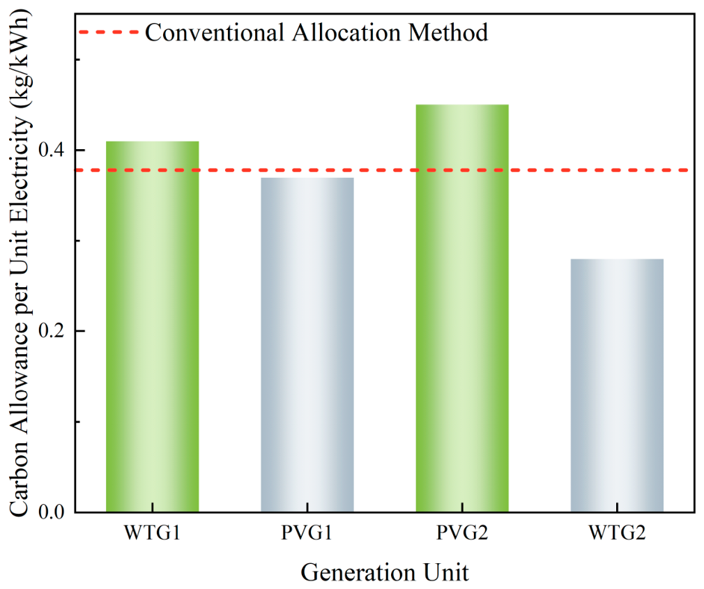
In conventional allocation methods, the carbon allowance per unit electricity generation of each DG is typically assigned as a fixed value based on historical experience. In this paper, a value of 0.39 kg/kWh is adopted as an example for comparative analysis. The carbon allowance allocation results for DG units under the Aumann–Shapley value method in Scheme 3 are illustrated in Figure 6. It can be observed that the unit carbon allowances of different DG units vary significantly, indicating that the Aumann–Shapley value method can dynamically allocate carbon responsibilities according to DG output levels and their marginal impacts on system carbon emissions. DG units with higher renewable energy penetration and greater low-carbon contributions are assigned lower carbon responsibilities, whereas DG units undertaking more power supply tasks during high-load periods and exhibiting higher marginal carbon emissions bear higher carbon responsibilities. This mechanism effectively guides the system toward prioritizing clean energy consumption, thereby optimizing overall system carbon emissions.

5.4. Analysis of Low-Carbon Distribution Network Expansion Planning Results

To evaluate the impacts of green certificate-tiered carbon trading based on the Aumann–Shapley value method and low-carbon demand response on distribution network expansion planning, four planning schemes are designed:

• Scheme 1: Neither green certificate-tiered carbon trading based on the Aumann–Shapley value method nor low-carbon demand response is considered;
• Scheme 2: Green certificate-tiered carbon trading based on the Aumann–Shapley value method is considered, while low-carbon demand response is not;
• Scheme 3: Low-carbon demand response is considered, while green certificate-tiered carbon trading based on the Aumann–Shapley value method is not;
• Scheme 4: Both green certificate-tiered carbon trading based on the Aumann–Shapley value method and low-carbon demand response are considered.

The cost components of the distribution network under each scheme are presented in

Table 5. Comparison of distribution network planning costs under different scenarios.

Scheme	Investment Cost (CNY)	Operating Cost (CNY)						Carbon Emissions (t)	Total Planning Cost (CNY)
		O&M	Electricity Purchasing	Network Loss	WTG and PVG Curtailment Penalty	Carbon Trading	DR
Scheme 1	5,169,103.4	3,831,871.5	8,374,022.7	254,937.6	373,857.8	1,621,379.1	—	6296.9	19,625,172.1
Scheme 2	6,045,574.4	5,309,593.2	6,955,477.3	261,353.6	122,469.5	895,871.2	—	5356.3	19,590,339.2
Scheme 3	5,373,707.4	4,548,941.5	5,853,973.7	252,721.9	197,458.6	1,413,279.3	876,271.4	5611.6	18,516,353.8
Scheme 4	6,231,825.6	5,689,593.2	4,497,176.4	249,848.3	118,017.3	984,242.3	1,345,761.5	4491.4	19,116,464.6

, and the corresponding planning configurations are shown in

Table 6. Distribution network planning configurations under different scenarios.

Scheme	New Lines	WTG Locations (Units)	PVG Locations (Units)	ESS Locations (Units)	Charging Facility Locations by Type (Units)
					SCF	FCF	UCF
Scheme 1	25–34 22–35 9–36 15–37	14( 5) 32 (4)	21( 2) 25 (4)	13 (1) 19 (1)	5 (11) 11 (11) 16( 9) 27( 8)	5 (3) 11 (3) 16 (4) 27 (3)	5 (1) 11 (2) 16 (1) 27 (1)
Scheme 2	25–34 22–35 9–36 15–37	14 (5) 32 (5)	21 (5) 25 (5)	13 (5) 19 (5)	5 (11) 11 (13) 16 (7) 27 (8)	5 (3) 11 (3) 16 (3) 27 (4)	5 (2) 11 (2) 16 (1) 27 (2)
Scheme 3	25–34 22–35 9–36 15–37	14 (5) 32 (5)	21 (3) 25 (4)	13 (2) 19 (3)	5 (12) 11 (9) 16 (8) 27 (7)	5 (4) 11 (5) 16 (2) 27 (3)	5 (2) 11 2) 16 (1) 27 (1)
Scheme 4	25–34 22–35 9–36 15–37	14 (5) 32 (5)	21 (5) 25 (5)	13 (5) 19 (5)	5 (9) 11 (16) 16 (6) 27 (9)	5 (3) 11 (3) 16 (3) 27 (3)	5 (3) 11 (1) 16 (2) 27 (2)

.

5.4.1. Analysis of the Impacts of the Green Certificate-Tiered Carbon Trading Mechanism Based on the Aumann–Shapley Value Method on System Performance

By comparing Scheme 1 and Scheme 2, it can be observed that after introducing the green certificate-tiered carbon trading mechanism based on the Aumann–Shapley value method, the installed capacities of WTG and PVG in the system increase significantly, indicating that the proposed mechanism can effectively enhance the motivation of the distribution network to utilize DG. In Scheme 1, since green certificate and carbon trading constraints are not considered, the system planning process mainly focuses on traditional economic objectives. Consequently, part of the load is still primarily supplied through electricity purchases from the main grid, resulting in a relatively low DG installation scale. In contrast, Scheme 2 introduces a green certificate mechanism and tiered carbon cost constraints, which enhance the environmental value of DG. As a result, the system proactively increases the installed capacities of DG during the planning stage to reduce carbon trading costs during operation.

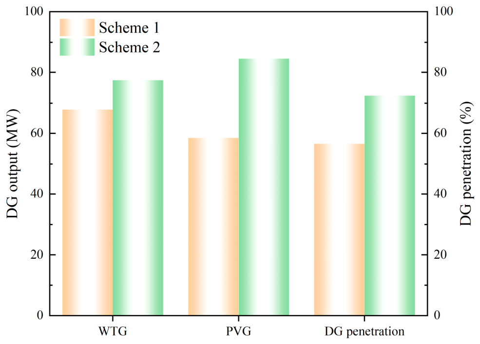
As further illustrated in Figure 7, after introducing the green certificate-tiered carbon trading mechanism based on the Aumann–Shapley value method, the DG-related indicators of the system are significantly improved. Specifically, the system carbon emissions decrease by approximately 14.9% compared with Scheme 1, indicating that the proposed mechanism can effectively improve the overall low-carbon operation level of the system. Meanwhile, the DG penetration rate increases from 56.6% to 72.5%, demonstrating that a larger proportion of the load is supplied by DG. This not only reduces the system’s dependence on electricity purchased from the main grid but also improves DG accommodation capability.

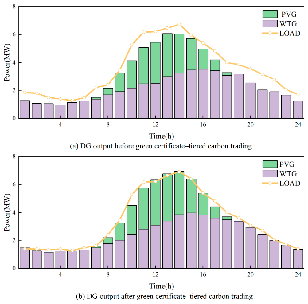
The DG output profiles shown in Figure 8 further indicate that, after considering the Aumann–Shapley value method, the overall DG output level increases significantly. In particular, WTG and PVG undertake more power supply tasks during peak load periods. This is mainly because the Aumann–Shapley value method can allocate carbon emission responsibilities more fairly and reasonably according to the marginal contribution of each participant to system carbon emissions, thereby more accurately reflecting the low-carbon advantages of renewable energy units.

5.4.2. Analysis of the Impacts of Low-Carbon Demand Response on System Performance

By comparing Scheme 1 and Scheme 3, it can be observed that the system operation mode changes significantly after introducing low-carbon demand response. In Scheme 1, low-carbon demand response is not considered, and user loads are mainly distributed according to their original electricity consumption habits. Consequently, the system still needs to purchase a large amount of electricity during high-load and high-carbon-emission periods to satisfy power supply demand, resulting in relatively high electricity purchasing costs and carbon emission levels during peak periods. In contrast, Scheme 3 introduces a low-carbon demand response mechanism based on dynamic carbon emission factors, which associates system carbon emission intensity with time-of-use electricity prices. This enables users to actively adjust their electricity consumption behavior according to the carbon emission levels of different periods, thereby achieving optimal load regulation over time.

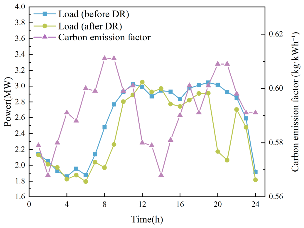
As shown in Figure 9, after implementing low-carbon demand response, the system load curve becomes noticeably smoother compared with the original load curve. The load peak during high-carbon-emission periods decreases significantly, while part of the load is shifted to low-carbon-emission periods. The primary reason is that, during high-carbon-emission periods, the electricity price corresponding to the dynamic carbon emission factor becomes relatively high. To reduce electricity consumption costs, transferable user-side loads tend to avoid high-carbon periods and shift toward periods with higher DG output and lower carbon emission levels. In addition, the relationship between the dynamic carbon emission factor and load variation indicates a strong coupling characteristic. When the dynamic carbon emission factor is high, the system load tends to decrease; conversely, when the carbon emission factor declines, the system load correspondingly increases. This demonstrates that the proposed low-carbon demand response model can effectively respond to carbon emission signals and achieve dynamic load adaptation to system carbon emission levels, thereby guiding users to participate in low-carbon system operation.

5.4.3. Analysis of the System Impacts of the Proposed Coordinated Mechanisms

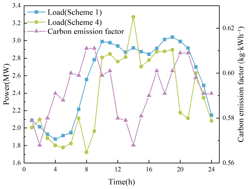
As shown in Figure 10, there are significant differences in load distribution characteristics between Scheme 1 and Scheme 4.

In Scheme 1, neither the green certificate-tiered carbon trading mechanism based on the Aumann–Shapley value method nor low-carbon demand response is considered. Therefore, the system load is mainly influenced by the original electricity consumption behavior of users, exhibiting a pronounced peak concentration phenomenon. During the periods of 9:00–12:00 and 17:00–21:00, the system load remains at a relatively high level, with the daily peak load occurring around 18:00–20:00. Under such conditions, the system typically needs to dispatch more high-carbon power sources to satisfy electricity demand, resulting in higher system carbon emissions.

In contrast, Scheme 4 comprehensively considers the green certificate-tiered carbon trading mechanism based on the Aumann–Shapley value method together with low-carbon demand response. By introducing dynamic carbon emission factors into the electricity price regulation process, users are encouraged to actively adjust their electricity consumption behavior according to the carbon emission intensity of different periods. During high-carbon-emission periods, the dynamic electricity price increases accordingly, motivating part of the transferable load to shift toward periods with lower carbon emission factors. As illustrated in Figure 8, during periods with relatively high dynamic carbon emission factors, such as 8:00–10:00 and 18:00–21:00, the load level in Scheme 4 is significantly lower than that in Scheme 1. Conversely, during periods with lower carbon emission factors, such as 13:00–16:00, part of the load is shifted to these intervals, resulting in increased load levels. This demonstrates that low-carbon demand response can effectively suppress load peaks during high-carbon periods and improve system load distribution characteristics. Moreover, the system planning cost in Scheme 4 is further reduced, while the system carbon emissions decrease by 25.9% compared with Scheme 1, indicating that the proposed mechanism can achieve more effective carbon emission reduction while maintaining economic performance.

5.4.4. Analysis of ESS Operating Characteristics

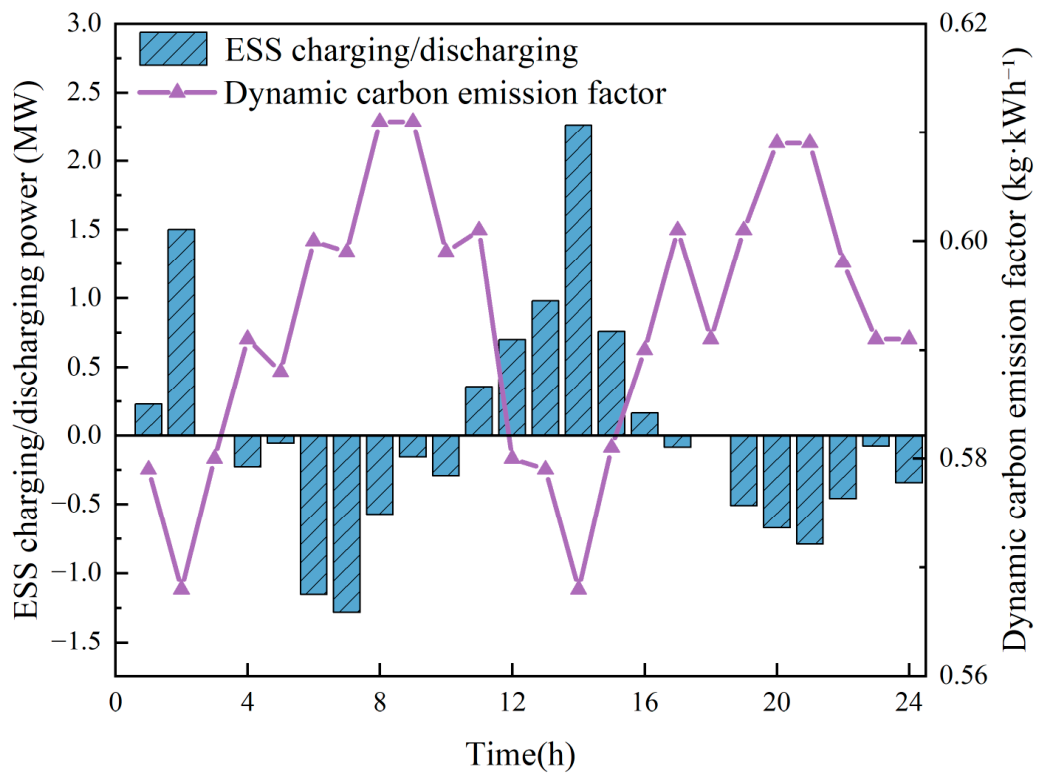
After considering the green certificate-tiered carbon trading based on the Aumann–Shapley value method mechanism and low-carbon demand response, the charging and discharging behavior of the ESS is affected to a certain extent, exhibiting a clear temporal correlation with the dynamic carbon emission factor. As shown in Figure 11, the charging and discharging profiles of the ESS are presented.

During periods with low dynamic carbon emission factors, the ESS operates in the charging mode to store energy, thereby providing support for subsequent high-carbon periods. In contrast, during periods with high carbon emission factors, the ESS discharges to supply power, which helps reduce carbon emissions during system operation while alleviating the supply pressure during peak load periods.

Overall, the ESS charging and discharging strategy takes into account the characteristics of the dynamic carbon emission factor, enabling a charging/discharging schedule that satisfies low-carbon operational requirements. The above analysis indicates that the ESS actively participates in the carbon reduction process of the distribution network by storing energy during low-carbon-intensity periods and supplying power during high-carbon-intensity periods.

5.5. Sensitivity Analysis of Key Parameters in the Carbon Trading Mechanism

To further investigate the impacts of key parameters in the green certificate-tiered carbon trading mechanism based on the Aumann–Shapley value method on system planning results, the carbon trading base price, carbon emission interval length, and carbon trading cost growth rate are selected as sensitivity analysis variables to analyze the variations in system planning cost and carbon emissions.

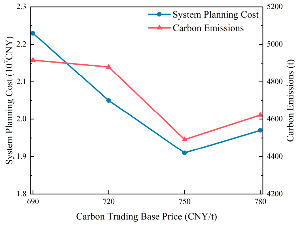
As shown in Figure 12, with the increase in the carbon trading base price, both the system planning cost and carbon emissions exhibit a trend of first decreasing and then increasing. When the carbon trading base price increases from 690 CNY/t to 750 CNY/t, both the system planning cost and carbon emissions decrease. This indicates that an appropriate increase in carbon price can strengthen carbon cost constraints and encourage the system to prioritize DG dispatch, thereby improving both economic performance and low-carbon operation. However, when the carbon trading base price further increases to 780 CNY/t, both the system planning cost and carbon emissions rise again. This is because excessively high carbon prices significantly increase the system carbon trading cost, thereby reducing the overall operational economic performance of the system.

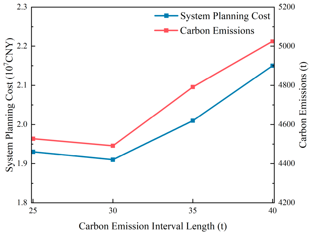
As illustrated in Figure 13, when the carbon emission interval length increases from 25 t to 30 t, both the system planning cost and carbon emissions slightly decrease, indicating that an appropriately larger carbon emission interval can reduce short-term operational pressure and improve system flexibility. However, when the interval length continues to increase, both the system planning cost and carbon emissions rise significantly. The main reason is that a larger carbon emission interval weakens the penalty intensity of the tiered carbon trading mechanism on high-carbon behaviors, thereby reducing the incentives for DG accommodation and low-carbon load regulation.

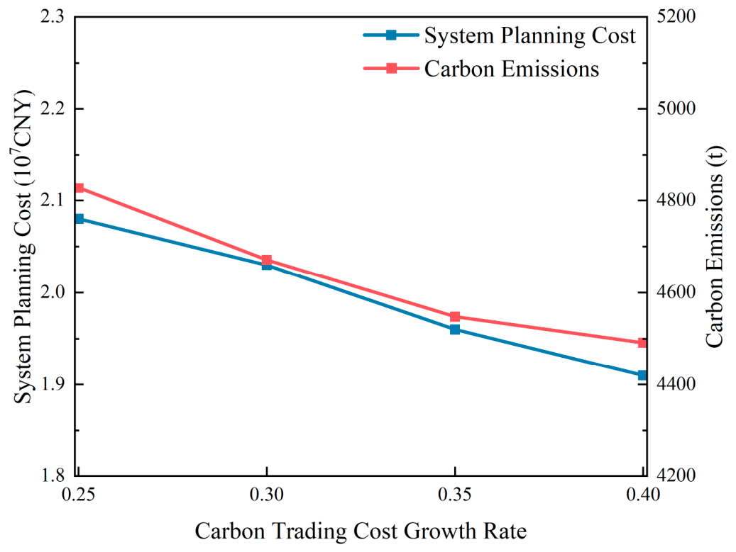
As shown in Figure 14, when the carbon trading cost growth rate increases from 0.25 to 0.40, the system planning cost gradually decreases from CNY 20.8 million to CNY 19.1 million, while carbon emissions decrease from 4827.2 t to 4491.4 t, representing a reduction of approximately 8.3%. Both indicators exhibit a monotonic decreasing trend. This demonstrates that a higher carbon trading cost growth rate strengthens the incentive effect of carbon price signals, encouraging the system to proactively implement emission reduction measures during the planning stage and increase renewable energy utilization, thereby achieving carbon reduction objectives.

6. Conclusions

To address the challenges of large-scale EV integration and low-carbon distribution network planning, this paper proposes a low-carbon distribution network expansion planning model considering the integration of multi-type EV charging facilities, based on a green certificate-tiered carbon trading mechanism incorporating the Aumann–Shapley value method. The main conclusions are as follows:

• The proposed distribution network planning model can realize the coordinated configuration of multi-type EV charging facilities according to EV state of charge and charging demand characteristics. Under the considered case-study conditions, compared with the single-type charging facility configuration scheme, the proposed method can reduce the system planning cost to a certain extent while satisfying EV charging demand, demonstrating favorable economic performance and configuration rationality.
• Under the considered simulation scenarios, the green certificate-tiered carbon trading mechanism based on the Aumann–Shapley value method can further reduce system carbon emissions and promote the consumption of distributed energy resources compared with conventional methods. The proposed mechanism exhibits positive effects on improving the low-carbon operation level and economic performance of the distribution network.

In addition, the proposed bi-level low-carbon expansion planning framework exhibits good generality and scalability. Although this study is mainly validated on a modified IEEE 33-bus radial distribution network, the developed models for coordinated planning of multi-type EV charging facilities, green certificate–tiered carbon trading, and low-carbon demand response can be further extended to larger-scale distribution systems. For scenarios with high EV penetration, the computational complexity is reduced to some extent through typical-day scenario modeling, SOCR convexification, and MISOCP reformulation, thereby providing satisfactory computational performance. Meanwhile, the proposed method still has potential applicability in weakly meshed networks, hybrid AC/DC systems, and scenarios with high penetration of renewable energy and energy storage systems. Such extensions can be achieved by further considering loop network operation constraints, AC/DC coupling constraints, and more sophisticated uncertainty modeling. Future work will focus on engineering validation based on practical regional distribution systems and further investigate large-scale stochastic EV charging behavior, multi-timescale coordinated optimization, and distributed solution methods to enhance the practical applicability and robustness of the proposed model.

References

1. Balu, K.; Mukherjee, V. Optimal Deployment of Electric Vehicle Charging Stations, Renewable Distributed Generation with Battery Energy Storage and Distribution Static Compensator in Radial Distribution Network Considering Uncertainties of Load and Generation. Appl. Energy 2024, 359, 122707. [Google Scholar] [CrossRef]
2. Du, B.; Jia, H.; Zhang, B.; Li, Y.; Wang, H.; Yan, J.; Du, E.; Zhang, N. Evaluating the Carbon-Emission Reduction Potential of Employing Low-Carbon Demand Response to Guide Electric-Vehicle Charging: A Chinese Case Study. Appl. Energy 2025, 397, 126196. [Google Scholar] [CrossRef]
3. Wu, Y.; Chen, Y.; Li, Z.; Golshannavaz, S. Robust Co-Planning of Distributed Photovoltaics and Energy Storage for Enhancing the Hosting Capacity of Active Distribution Networks. Renew. Energy 2025, 253, 123645. [Google Scholar] [CrossRef]
4. Mirhoseini, S.P.; Hashemi, S.M. A Novel Approach for Battery Energy Storage Systems Expansion Planning in Distribution Network. J. Energy Storage 2025, 138, 118565. [Google Scholar] [CrossRef]
5. Jooshaki, M.; Abbaspour, A.; Fotuhi-Firuzabad, M.; Munoz-Delgado, G.; Contreras, J.; Lehtonen, M.; Arroyo, J.M. An Enhanced MILP Model for Multistage Reliability-Constrained Distribution Network Expansion Planning. IEEE Trans. Power Syst. 2022, 37, 118–131. [Google Scholar] [CrossRef]
6. Li, J.; Li, F.; Sun, K.; Sun, B. Bi-Level Coordinated Expansion Planning of High-PV-Penetration Active Distribution Networks Incorporating Multiple Flexible Resources Considering WGAN-GP-Based Uncertainty Generation. Energy 2025, 330, 136685. [Google Scholar] [CrossRef]
7. Feng, P.; Chen, C.; Wang, L. Coordinated Energy Storage and Network Expansion Planning Considering the Trustworthiness of Demand-Side Response. Front. Energy Res. 2024, 12, 1384760. [Google Scholar] [CrossRef]
8. Lin, J.; Sun, J.; Feng, Y.; Zheng, M.; Yu, Z. Aggregate Demand Response Strategies for Smart Communities with Battery-Charging/Switching Electric Vehicles. J. Energy Storage 2023, 58, 106413. [Google Scholar] [CrossRef]
9. Kabirifar, M.; Fotuhi-Firuzabad, M.; Moeini-Aghtaie, M.; Pourghaderi, N.; Shahidehpour, M. Reliability-Based Expansion Planning Studies of Active Distribution Networks with Multiagents. IEEE Trans. Smart Grid 2022, 13, 4610–4623. [Google Scholar] [CrossRef]
10. Adetunji, K.E.; Hofsajer, I.W.; Abu-Mahfouz, A.M.; Cheng, L. An Optimization Planning Framework for Allocating Multiple Distributed Energy Resources and Electric Vehicle Charging Stations in Distribution Networks. Appl. Energy 2022, 322, 119513. [Google Scholar] [CrossRef]
11. Cai, S.; Xie, Y.; Tian, W.; Wu, Q. Resilient Microgrid Formation in Unbalanced AC/DC Hybrid Distribution System Considering DC Interconnections. Electr. Power Syst. Res. 2026, 251, 112274. [Google Scholar] [CrossRef]
12. Ding, T.; Lu, R.; Xu, Y.; Yang, Q.; Zhou, Y.; Zhang, Y.; Wen, Y. Joint Electricity and Carbon Market for Northeast Asia Energy Interconnection. Glob. Energy Interconnect. 2020, 3, 99–110. [Google Scholar] [CrossRef]
13. Castro, F.; Canizes, B.; Soares, J.; Almeida, J.; Vale, Z. Comprehensive Framework for Distribution Network Multi-Investment Expansion Planning: Emissions, Uncertainty, and Resource Remuneration Integration. Energy Convers. Manag. 2024, 316, 118734. [Google Scholar] [CrossRef]
14. Liu, Z.; Xing, H.; Luo, Y.; Ye, Y.; Shi, Y. Low-Carbon Economic Dispatch of an Integrated Energy System Based on Carbon Emission Flow Theory. J. Electr. Eng. Technol. 2023, 18, 1613–1624. [Google Scholar] [CrossRef]
15. Wang, B.; Li, C.; Ban, Y.; Zhao, Z.; Wang, Z. A Multi-Market Equilibrium Model Considering the Carbon-Green Certificate Mutual Recognition Trading Mechanism under the Electricity Market. Energy 2025, 330, 136902. [Google Scholar] [CrossRef]
16. Junqueira, M.; da Costa, L.C.; Barroso, L.A.; Oliveira, G.C.; Thome, L.M.; Pereira, M.V. An Aumann-Shapley Approach to Allocate Transmission Service Cost Among Network Users in Electricity Markets. IEEE Trans. Power Syst. 2007, 22, 1532–1546. [Google Scholar] [CrossRef]
17. Hamed, A.; Torky, M.; AlJanah, S.; Alshammari, A.; Gaber, T. A Blockchain-Based Fox Optimization Algorithm for Optimizing and Securing Electrical Vehicles Charging. IEEE Trans. Intell. Veh. 2025, 10, 4479–4498. [Google Scholar] [CrossRef]
18. Dahiwale, P.V.; Rather, Z.H.; Mitra, I. A Comprehensive Review of Smart Charging Strategies for Electric Vehicles and Way Forward. IEEE Trans. Intell. Transp. Syst. 2024, 25, 10462–10482. [Google Scholar] [CrossRef]
19. Ameer, H.; Wang, Y.; Chen, Z. A Density-Based Spatial Clustering and Linear Programming Method for Electric Vehicle Charging Station Location and Price Optimization. Energy 2025, 317, 134581. [Google Scholar] [CrossRef]
20. Christensen, K.; Ma, Z.G.; Jørgensen, B.N. A Scoping Review on Electric Vehicle Charging Strategies with a Technical, Social, and Regulatory Feasibility Evaluation. Renew. Sustain. Energy Rev. 2025, 211, 115300. [Google Scholar] [CrossRef]
21. Tao, Y.; Qiu, J.; Lai, S.; Sun, X.; Zhao, J. Adaptive Integrated Planning of Electricity Networks and Fast Charging Stations Under Electric Vehicle Diffusion. IEEE Trans. Power Syst. 2023, 38, 499–513. [Google Scholar] [CrossRef]
22. Li, H.; Azzouz, M.A.; Hamad, A.A. Cooperative Voltage Control in MV Distribution Networks with Electric Vehicle Charging Stations and Photovoltaic DGs. IEEE Syst. J. 2021, 15, 2989–3000. [Google Scholar] [CrossRef]
23. Pal, A.; Bhattacharya, A.; Chakraborty, A.K. Planning of EV Charging Station with Distribution Network Expansion Considering Traffic Congestion and Uncertainties. IEEE Trans. Ind. Appl. 2023, 59, 3810–3825. [Google Scholar] [CrossRef]
24. Jiang, X.; Chen, J.; Zhang, W.; Wu, Q.; Zhang, Y.; Liu, J. Two-Step Optimal Allocation of Stationary and Mobile Energy Storage Systems in Resilient Distribution Networks. J. Mod. Power Syst. Clean Energy 2021, 9, 788–799. [Google Scholar] [CrossRef]
25. Liao, J.; Wu, G.; Lin, J. Linearized MILP Model with Improved Soft Actor-Critic Algorithm for Dynamic and Efficient Active Distribution Network Planning. IEEE Access 2025, 13, 121544–121555. [Google Scholar] [CrossRef]
26. Cuenca, J.J.; Vanin, M.; Hashmi, M.U.; Koirala, A.; Ergun, H.; Hayes, B.P. Event-Informed Identification and Allocation of Distribution Network Planning Candidates with Influence Scores and Binary Linear Programming. IEEE Trans. Power Syst. 2025, 40, 492–504. [Google Scholar] [CrossRef]
27. Liu, Z.; Liu, H.; Xu, Z.; Li, R.; Guo, Y.; Du, Y. Differentiated Reliability-Based Regional Distribution Network Planning with Probability Characteristics of PV and Load. IEEE Trans. Ind. Appl. 2025, 61, 4613–4625. [Google Scholar] [CrossRef]
Figure 1. Distribution curves of EV arrival quantity and dwell time.
Energies 19 02638 g001
Figure 2. Bi-level expansion planning framework of the distribution network.
Energies 19 02638 g002
Figure 3. Solution procedure of the proposed model.
Energies 19 02638 g003
Figure 4. Topology of the modified IEEE 33-bus distribution network.
Energies 19 02638 g004
Figure 5. Wind–PV–load power profiles under a typical daily scenario.
Energies 19 02638 g005
Figure 6. Carbon allowance allocation results of DG units.
Energies 19 02638 g006
Figure 7. Comparison of key results with and without green certificate-tiered carbon trading.
Energies 19 02638 g007
Figure 8. The output situation of distributed generation.
Energies 19 02638 g008
Figure 9. Load profiles before and after implementing low-carbon demand response.
Energies 19 02638 g009
Figure 10. Load power shifting profiles under different scenarios.
Energies 19 02638 g010
Figure 11. Charging and discharging profiles of energy storage systems.
Energies 19 02638 g011
Figure 12. Impact of carbon trading base price.
Energies 19 02638 g012
Figure 13. Impact of carbon emission interval length.
Energies 19 02638 g013
Figure 14. Impact of carbon trading cost growth rate.
Energies 19 02638 g014