Ship Electric Propulsion Based on Hydrogen Fuel Cell, Batteries, PVs and WASP: Energy Management, Dynamics and Converter-Driven Stability

Abstract

This paper presents a complete analysis and simulation of the operation of a zero-emission marine vessel with electric propulsion. A hypothetical passenger ferry operating in the Aegean Sea, Greece, is considered, which is powered by a hydrogen fuel cell, a battery energy storage system (BESS) and photovoltaic (PV) energy. Wind-assisted ship propulsion (WASP) is employed to reduce the energy consumption of the ship. A complete analysis is performed, which includes optimal energy management, dynamic analysis and emerging stability concerns due to the high integration of power electronic converters in the shipboard microgrid. The energy management system (EMS) applies multi-objective optimization based on the corona virus optimization (CVO) algorithm and the teaching–learning-based optimization algorithm (TLBO). The dynamic behavior of the microgrid is tested using real-time digital simulations. Converter-driven stability issues are investigated, which may arise due to interactions among the various converter controllers and passive components of the microgrid.

1. Introduction

Shifting to sustainable energy in power generation, transportation, heating, and cooling is one of the major challenges of our time. The shipping industry carries around 80% of global trade by volume and contributes nearly 3% of the global greenhouse gas emissions. In 2023, the International Maritime Organization (IMO) announced important decarbonization targets to accelerate the decarbonization process of the shipping industry [1]. The transition is taking place from fossil-fuel-based mechanical propulsion towards alternative energy technologies and hybrid and electrification technologies. Propulsion electrification is playing an increasingly important role, allowing for hybrid solutions in the electricity generation/storage side and the operation of intelligent shipboard microgrids. Green hydrogen is an emerging alternative fuel that can generate electric power through fuel cells, but it has disadvantages such as low volumetric energy density, storage challenges and high production cost. The development of durable and cost-effective fuel cells will play an important role in the decarbonization of the shipping industry, supported by recent advancements in proton exchange membranes [2] and other technologies. Battery energy storage systems (BESS) are used already in short-route electric ships but have limitations such as low energy density and high weight. Photovoltaic (PV) energy, especially in areas with high solar irradiation, can supplement the energy production, but the low efficiency and limited space on ships impose important constraints. Wind energy can contribute with wind-assisted ship propulsion (WASP) technologies, such as rotor sails, wing sails and kites, reducing fuel consumption and operational cost; however, the high investment cost and complexity of these solutions remain key challenges. Overall, a combination of technologies is needed, as well as proper energy management systems (EMS) to optimize the operation of the emerging shipboard microgrids.

The energy management of shipboard microgrids with fuel cells, BESS and renewable/conventional generation has been investigated in many publications. Representative review papers and applications from the recent literature are presented below. The state of the art of EMS for hybrid fuel cell applications in ships is reviewed in [3], focusing on various strategies, including optimization-based, rule-based, and learning-based approaches. A review of EMS of shipboard microgrids is provided in [4], covering traditional methods, such as evolutionary algorithms, model predictive control, fuzzy logic control, and more modern approaches, such as machine learning and deep learning. EMS and converter topologies of marine hybrid energy storage systems are reviewed in [5]. In a similar line, EMS for fuel cell hybrid ships are classified and compared in [6,7].

A review of optimization-based power management and EMS for shipboard microgrids is provided in [8]. An improved sine cosine algorithm is used for the power dispatch optimization of a ferry boat based on fuel cell, battery, and cold ironing [9]. Particle swarm optimization is applied in the EMS of a fuel cell/battery ship, considering power quality aspects [10]. A real-time optimization-based EMS for fuel cell hybrid ships is proposed in [11], considering the degradation of the power sources. A two-layer, multi-objective EMS based on model predictive control is proposed in [12] to achieve economical and efficient operation of hybrid fuel cell–battery ships. A multi-objective optimization based EMS using model predictive control is developed in [13], which aims to balance fuel use and load-induced degradation of the fuel cells.

Rule-based EMS are presented next. The performance of a fuzzy logic rule-based EMS strategy for a hybrid fuel cell powered passenger vessel is investigated in [14] to reduce hydrogen consumption. An EMS with two fuzzy logic controllers for a shipboard microgrid is proposed in [15], including solar panels, windmills, a fuel cell, a diesel generator, and energy storage devices. An improved fuzzy-based EMS for a tourist ship microgrid is proposed in [16], including a fuel cell, PVs, a battery and super-capacitors. A two-layer energy management system for a hybrid electrical passenger ship with multi-PEM fuel cell stack is proposed in [17], which combines the global optimization and rule-based method to realize near-global optimal solutions. An EMS of the DC microgrid of a smart yacht is presented in [18], including diesel generators, a fuel cell, PVs, a wind turbine and a battery storage system.

Moreover, machine learning techniques are applied in the EMS of shipboard microgrids. A neural-network-based EMS for hybrid fuel cell/battery powered ships is proposed in [19], considering fuel cell degradation. A double Q reinforcement learning-based EMS for a plug-in hybrid fuel cell and battery ships is proposed in [20] to achieve near-optimal average voyage cost. An EMS for fuel cell hybrid ships using deep Q-learning is presented in [21] to optimize voyage cost, fuel cell lifespan, and battery stage of charge. A two-layer EMS based on prior knowledge of fuel cell hybrid ship operation is applied in [22], using dynamic programming, low-pass filtering, neural network training and a support vector machine. An optimized power management strategy to reduce the total cost (fuel cost, emission penalty, power device degradation, equipment replacement cost) of a DC shipboard microgrid is applied in [23] using model predictive control and reinforcement learning.

As outlined above, several publications consider heuristic methods for the EMS of shipboard microgrids, such as particle swarm optimization and sine cosine algorithm, among others. Corona virus optimization (CVO) was proposed for the first time in 2020, inspired by the global pandemic [24,25]. CVO has gained attention on terrestrial power systems in the last several years. It has been applied for the optimal operation of the Egyptian Power System [26] and the Iraqi Power System [27], for the static and dynamic optimal power flow of the IEEE 30 bus system [28], and for power system load–frequency–control [29], among others. Earlier, in 2011–2012, the teaching–learning-based optimization (TLBO) was introduced [30] and has also been applied in several terrestrial power system studies, such as [31,32,33]. However, the application of the CVO and the TLBO for the energy management of shipboard power systems has not been investigated until now. Moreover, an important issue is the convergence behavior and parameter identification limitations of metaheuristic algorithms in complex fuel cell hybrid systems. In [34] a multi-strategy tuna swarm optimization (TSO) was proposed to estimate the parameters of proton exchange membrane fuel cell (PEMFC) voltage models based on measured data and was compared with other algorithms, such as differential evolution, the whale optimization approach, etc. Overall, TSO can perform better in forecasting and estimation problems, while CVO and TLBO are expected to perform better in operational aspects of microgrids and power systems.

EMS systems analyze the shipboard microgrid in steady-state conditions. Dynamic simulation and stability analysis, to ensure the stable operation of the system, are often overlooked in EMS-related publications. Converter-driven stability has been recognized as an emerging stability issue in terrestrial power systems and has been added as a new category in the recent stability classification of IEEE [35,36]. Converter-interfaced generation/storage and loads are equipped with multiple control schemes, which have been reported to interact with passive grid components and other power electronic devices, leading to unstable oscillations in low frequencies, close to the nominal, but also much higher frequencies (100 Hz–kHz). High-frequency oscillations, classified as fast-interaction converter-driven stability in [35,36], can arise from the interaction between the fast current controllers of the converters connected at close proximity [37]. Fast-interaction converter-driven stability issues have been analyzed in the bulk power system [38,39] but also in terrestrial microgrids [40]. However, fast-interaction converter-driven stability for AC shipboard microgrids has not been analyzed yet. Shipboard microgrids include several power electronic converters for integrating generation, storage and propulsion technologies, as well as heating, ventilation and air conditioning (HVAC) systems, auxiliary motors, etc. Therefore, such an analysis is useful for shipboard microgrids rich in power electronic converters, such as the one considered in this paper.

In this paper a complete analysis of the shipboard microgrid is performed, including energy management, dynamic analysis and emerging stability concerns due to the increased integration of power electronic converters.

The main contributions of this work are as follows:

• The CVO and TLBO optimization techniques are applied for the first time for the energy management of shipboard microgrids.
• Fast-interaction converter-driven stability is investigated for the first time for AC shipboard microgrids.

This paper is structured as follows. Section 2 presents the configuration and modeling of the different components of the shipboard microgrid. Section 3 describes the energy management system, using both CVO and TLBO algorithms. Section 4 reports real-time dynamic simulations, including rapid load increase. Section 5 investigates converter-driven stability issues. Section 6 concludes the paper.

2. Microgrid Configuration

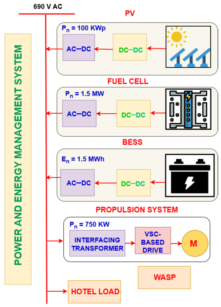
This paper considers a hypothetical zero-emission passenger ferry with electric propulsion operating in the Aegean Sea, Greece. The ferry is powered by a hydrogen fuel cell of 1.5 MW (including hydrogen storage tanks), a BESS of 1.5 MWh and PVs of 100 kW_p. WASP is employed to support ship propulsion and reduce fuel consumption. A 750 kW electric propulsion system is considered. The vessel is rich in renewable energy sources and does not use conventional fuels. A total daily trip duration of 10 h is considered, including 7 h sailing and 3 h anchored. Figure 1 shows a high-level overview of the shipboard microgrid.

The basic component equations are described next, which are used in the energy management system of Section 3.

2.1. Photovoltaic System

The 100 kW_p PV system is modeled as shown in (1).

$$P_{PV}={\eta }_{panel}·{\eta }_{inverter}·G·A_{PV}·(1-\beta \left(T_C-T_{ref}\right))$$

(1)

where ${\eta }_{inverter}$ is the inverter efficiency, $A_{PV}$ is the PV array area in the marine vessel in m², $G$ is the solar irradiation in W/m², ${\eta }_{panel}$ is the efficiency of the PV array, $\beta$ is the temperature coefficient, $T_C$ is the PV cell temperature and $T_{ref}$ is the reference cell temperature in Kelvin [41].

2.2. Hydrogen Storage and Fuel Cell

The system includes 53 hydrogen storage tanks, and each tank includes 6 kg of hydrogen. The PEMFC technology is considered. The 1.5 MW fuel cell system converts the stored hydrogen to electricity. The hydrogen storage system can be calculated as shown in (2).

$${\displaystyle \frac{V_{storage}(t)}{RT}}Pressure(t)=n_{storedhydrogen}$$

(2)

where $Pressure$ represents the pressure of the hydrogen gas, $V_{storage}$ is the volume of the stored hydrogen, $T$ is the temperature during the adiabatic process, and $R$ is the ideal gas constant.

The operation of the fuel cell system is modeled with the power utilized in the redox reaction, $P_{FC}$ shown in (3), and the amount of hydrogen consumed during this process, $m_{FC}$ shown in (4).

$$P_{FC}={\displaystyle {\sum }_{i=1}^{N_{FC}}}{A}_i^{FC}{I}_{FC}{V}_{FC}$$

(3)

where $A$ represents the operational status of the fuel cell (0 indicates off and 1 indicates on). $N_{FC}$ refers to the total number of fuel cells. The variables $V_{FC}$ and $I_{FC}$ represent the voltage and current of the fuel cell, respectively.

$$m_{FC}(t)={\displaystyle \frac{N_{FC}{I}_{FC}∆t}{2F}}M$$

(4)

$F$ is the Faraday constant, and the quantity $M$ refers to the molar mass of hydrogen in kilograms/moles [42].

It should be noted that degradation dynamics and lifetime prediction mechanisms of fuel cells are becoming increasingly important, as explained in [43], and will be considered in future work. Similarly, considering the complex dynamic interactions and high-frequency transient responses in shipboard microgrids, adaptive control design for the fuel cell (e.g., similar to [44]) will be considered in future work.

2.3. Battery Energy Storage System

The microgrid is designed to have 1.5 MWh BESS. The BESS is modeled as in (5).

$$E_B\left(t+\Delta t\right)=E_B\left(t\right)+\Delta t(P_{Charging}\left(t\right)·{\eta }_{Charging}-{\displaystyle \frac{P_{Discharging}\left(t\right)}{{\eta }_{Discharging}}})$$

(5)

where $E_B\left(t\right)$ is the energy of the BESS, $\Delta t$ is the time step, and $P_{Charging}$ and $P_{Discharging}$ are the charging and discharging power, while ${\eta }_{Charging}$ and ${\eta }_{Discharging}$ are the charging and discharging efficiencies [45].

2.4. Wind-Assisted Ship Propulsion

WASP is employed to reduce fuel consumption [46,47]. A simplified model is used. The effective propulsion force of the WASP system $F_{Thrust}$ is calculated as follows [48].

$$F_{Thrust}=F_L\sin \beta -F_D\cos \beta$$

(6)

where $F_L$ and $F_D$ are the lift and drag forces, respectively, and $\beta$ is the apparent wind angle in degrees. Lift is the aerodynamic force generated perpendicular to the apparent wind direction that pulls the vessel forward, while drag is the force acting parallel to the wind that tends to oppose the ship’s motion [49].

The WASP power $P_{WASP}$ is calculated as follows, where $V_{ship}$ is the vessel speed [49].

$$P_{WASP}=F_{Thrurst}·V_{ship}$$

(7)

After applying the WASP effect, the required electric propulsion power ($P_{electric}$) from the microgrid can be approximated with Equation (8).

$$P_{electric}=P_{Propulsion}-P_{WASP}$$

(8)

where $P_{Propulsion}$ is the propulsion power required in absence of WASP.

3. Energy Management System

3.1. Overview

The proposed marine microgrid operates under a centralized EMS, responsible for the optimal active power dispatch of the fuel cell, BESS and PV. The control architecture is based on a supervisory control strategy operating over discrete time intervals t ∈ [1,T], where each time step represents 1 h of vessel operation along the route in the Aegean Sea. The simulations were executed with SAM 2025 software application.

3.2. Multi-Objective Optimization Formulation

The EMS aims to achieve the following objectives: minimum daily operation cost ($C_1)$, minimum renewable energy curtailment ($C_2$) and minimum fuel cell usage ($C_3$), as presented in (9), (10) and (11). The minimum daily operation cost objective (C₁) considers both hydrogen consumption and battery degradation.

$${minC}_1={\displaystyle {\sum }_{t=1}^T}(C_{H_2}·{\dot{m}}_{H_2}\left(t\right)+C_{deg}{P}_{discharging}\left(t\right))∆t;C_{deg}={\displaystyle \frac{C_{Bat}}{N_{Cycle}·2·{DoD}_{ref}·{\eta }_{Sys.}}}$$

(9)

$${minC}_2={\displaystyle {\sum }_{t=1}^T}{P}_{curt}\left(t\right)∆t$$

(10)

$${minC}_3={\displaystyle {\sum }_{t=1}^T}{P}_{FC}\left(t\right)∆t$$

(11)

$C_{deg}$ is the degradation cost, $C_{Bat}$ is the cost of battery replacement, and ${DoD}_{ref}$ is the reference depth of discharge specified by the battery manufacturer. ${\eta }_{Sys.}$ represents the lumped efficiency of the power electronics. $N_{Cycle}$ is the number of cycles the battery can handle before reaching 80% of its capacity. $P_{discharging}$ is the battery discharging power (kW).

$C_{H_2} \mathrm{i}\mathrm{s} \mathrm{t}\mathrm{h}\mathrm{e} \mathrm{u}\mathrm{n}\mathrm{i}\mathrm{t} \mathrm{c}\mathrm{o}\mathrm{s}\mathrm{t} \mathrm{o}\mathrm{f} \mathrm{h}\mathrm{y}\mathrm{d}\mathrm{r}\mathrm{o}\mathrm{g}\mathrm{e}\mathrm{n}(\mathrm{\$}/\mathrm{k}\mathrm{g}).{\dot{m}}_{H_2}$ is the hydrogen consumption rate at time t (kg/s), calculated as follows.

$${\dot{m}}_{H_2}(t)={\displaystyle \frac{P_{FC}\left(t\right)}{n_{FC}·{LHV}_{H_2}}}$$

(12)

where $P_{FC}$ is the fuel cell active power (kW), $n_{FC}$ is the fuel cell efficiency and ${LHV}_{H_2}$ is the lower heating value of hydrogen.

$P_{curt}$ is the curtailed power of the PVs.

To apply the multi-objective optimization a weighting factor is assigned to each objective, as shown in (13) and (14). $w_1$, $w_2$ and $w_3$ are the weighting factors of each objective and assumed to be equal in this study. ${\lambda }_k$ is a large penalty coefficient, which is 10⁶, and $g_k$ is the specific constraint violation.

$$minC=w_1{C}_1+w_2{C}_2+w_3{C}_3+{\sum }_k{\lambda }_k·{\mathrm{m}\mathrm{a}\mathrm{x}(0,g_k\left(x\right))}^2$$

(13)

$$w_1+w_2+w_3=1$$

(14)

The control variables are the fuel cell output power ($P_{FC}$), BESS discharging power ($P_{discharging}$) power, BESS charging power ($P_{charging}$), PV production and sail deployment ratio of the WASP.

The optimization process is subject to constraints as follows:

i.

Power balance constraint:

The total power generated must fulfill the total power consumed in the marine vessel, as stated in (15). Curtailed power is added to ensure balance even if the produced power is more than the needed power.

$$P_{PV}+P_{FC}+P_{discharging}=P_{Propulsion}-P_{WASP}+P_{Hotel}+P_{charging}+P_{curt}$$

(15)

ii.

Photovoltaic constraints:

The PV has maximum power $\left(P_{PV}^{maximum}\right)$ that can produce as presented in (16).

$${0\le P}_{PV}\le P_{PV}^{maximum}$$

(16)

iii.

BESS constraints:

The BESS has maximum charging power $\left(P_{charging}^{maximum}\right)$ and discharging power $\left(P_{discharging}^{maximum}\right)$ as presented in (17) and (18). No simultaneous charging and discharging is allowed based on (19). The limits of the state of charge (SOC) of the BESS are shown in (20).

$${0\le P}_{charging}\le P_{charging}^{maximum}$$

(17)

$${0\le P}_{discharging}\le P_{discharging}^{maximum}$$

(18)

$$P_{charging}\left(t\right)·P_{discharging}\left(t\right)=0$$

(19)

$$0.2\le SOC\left(t\right)\le 0.9$$

(20)

iv.

Hydrogen and fuel cell constraints:

The storage tanks in the vessel have limitations for storing the hydrogen energy, as presented in (21). Moreover, there are limitations for the operating power of the fuel cell, as shown in (22).

$$E_{H_{min}}\le E_H\left(t\right)\le E_{H_{max}}$$

(21)

$$P_{{FC}_{min}}\le P_{FC}\le P_{{FC}_{max}}$$

(22)

3.3. Corona Virus Optimization Algorithm

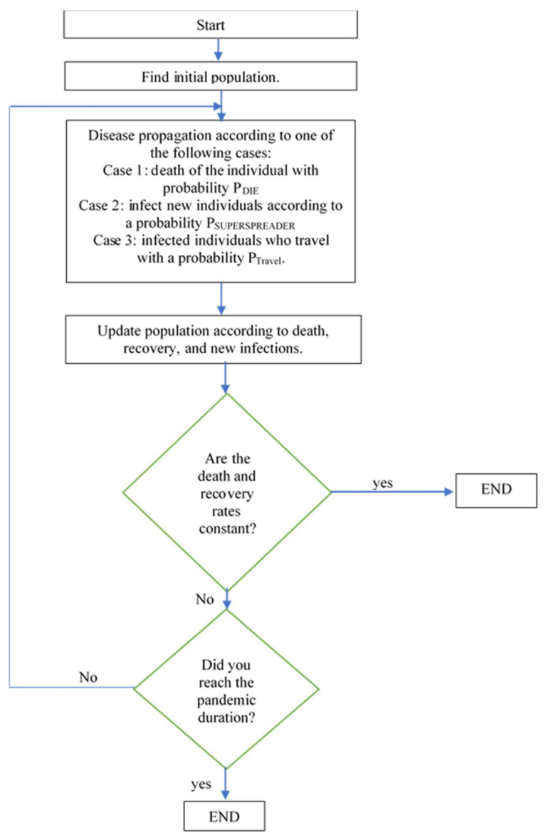
The CVO is a population-based metaheuristic optimization technique inspired by the epidemiological spread mechanism of viral transmission [24,25,26]. The algorithm mathematically mimics infection propagation, mutation, recovery, and immunity development to explore and exploit the search space efficiently.

Unlike classical evolutionary algorithms, CVO introduces infection-driven diversification and adaptive mutation mechanisms that enhance global search capability while maintaining convergence stability. Candidate solutions represent individuals in a population, and their fitness values determine infection strength and transmission probability. The mathematical modeling follows.

Let the population consist of N individuals, where each individual $X_i$ represents a candidate solution vector:

$$X_i=[x_{i1},x_{i2},\dots \dots \dots ,x_{id}]$$

(23)

where $d$ denotes the problem dimension.

-

Initialization:

$$x_{ij}=x_{jmin}+r(x_{jmax}-x_{jmin})$$

(24)

where r ∈ [0, 1] is a uniformly distributed random number.

-

Infection Phase:

Transmission probability Pt is defined as follows:

$$P_t=\min (1,\mathrm{m}\mathrm{a}\mathrm{x}(\beta ({\displaystyle \frac{f_{best}}{f_i+\epsilon }})))$$

(25)

where:

• $\beta$ is the infection rate, $f_{best}$ is the best fitness value, $f_i$ is the fitness of individual i and ε is a small constant.

The updated solution becomes

$$X_{inew}=X_i+\alpha \left(X_{best}-X_i\right)+\delta$$

(26)

where $\alpha$ is the transmission coefficient and $\delta$ is a mutation perturbation vector.

-

Mutation Mechanism:

$$\delta =\gamma \times N\left(\mathrm{0,1}\right)$$

(27)

where $\gamma$ is the mutation intensity and $N\left(\mathrm{0,1}\right)$ is a Gaussian distribution.

-

Recovery and Immunity:

Weak individuals are replaced by new random solutions to maintain diversity and avoid premature convergence.

The CVO flowchart is illustrated in Figure 2.

3.4. Teaching–Learning-Based Optimization Algorithm

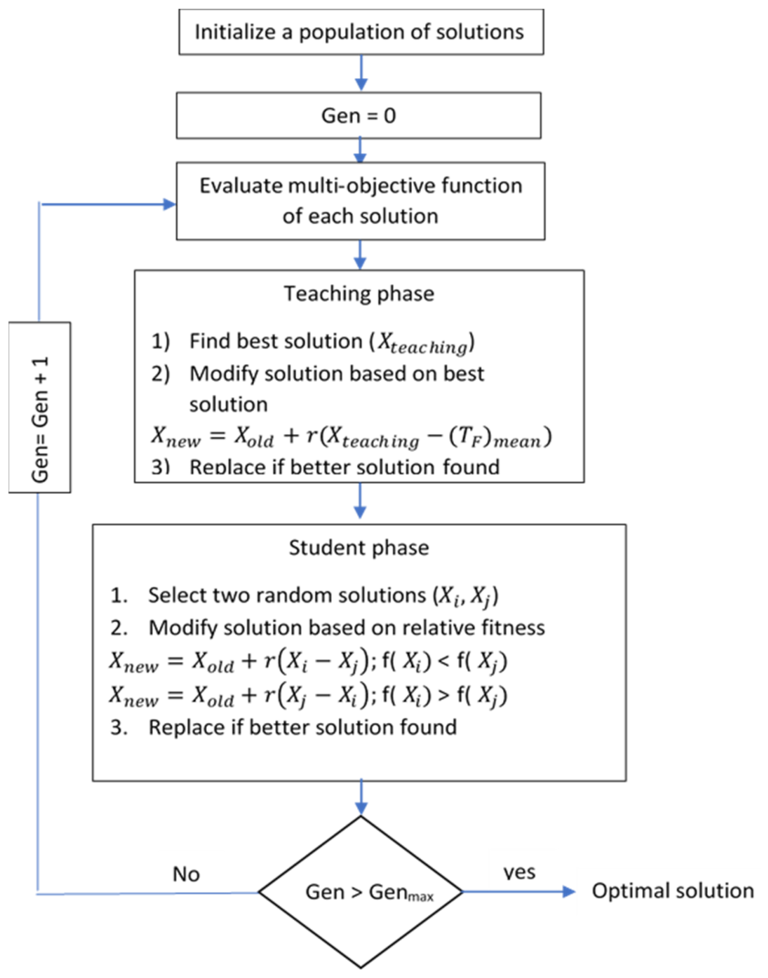
The TLBO is inspired by how students improve their knowledge through a teacher’s inputs and discussions with other students [26,30,31,32]. The students represent candidate solutions, subjects represent variables and the teacher represents the best solution in the population. Part of the mathematical formulation is summarized below.

-

Teacher phase:

The teacher tries to improve the mean knowledge of the class.

$$X_{new}=X_i+r(X_{teacher}-T_F·M)$$

(28)

where $X_i$ is the current solution (student), $X_{teacher}$ is the best solution, $M$ is the mean of the population, $T_F$ is the teaching factor (usually 1 or 2) and $r$ is a random number from 0 to 1. If the new solution is better, it replaces the old one.

-

Learner phase:

Two students are randomly selected, $X_i$ and $X_j$. If (29) is fulfilled, the data is updated according to (30). Otherwise, (31) is applied to ensure the survival of the best solution.

$$f\left(X_i\right)<f\left(X_j\right)$$

(29)

$$X_j^{new}=X_j+r(X_i-X_j)$$

(30)

$$X_i^{new}=X_i+r(X_j-X_i)$$

(31)

The TLBO flowchart is illustrated in Figure 3.

3.5. Optimization Results

This section reports the results of the EMS applied for the optimal operation of the passenger ferry. The multi-objective problem is solved using the two optimization techniques, namely, TLBO and CVO. Two vessel operational modes are considered: sailing and anchoring. During anchoring, the required energy is low (hotel load), which is supplied by the BESS and PVs. During sailing, the WASP reduces the propulsion load according to the environmental conditions. Moreover, the major part of the total load (propulsion and hotel load) is supplied by the fuel cell, supplemented by the BESS and PVs, according to the environmental conditions. Four study cases are considered for a daily round trip of the passenger ferry in the Aegean Sea: summer, spring, fall and winter.

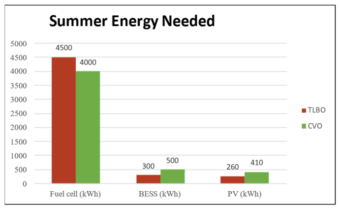
In summer, PVs produce more energy than the other seasons due to higher solar irradiation and longer daylight hours, supported by natural cooling during sailing. Moreover, the powerful “Meltemi” wind of the Aegean Sea during summer has a stronger effect on the reduction in propulsion power. Figure 4 shows that the energy provided by the fuel cell is approximately 4500 kWh using the TLBO and 4000 kWh using the CVO. The PV produced energy is 260 kWh in TLBO and 410 kWh in CVO. It is shown that the CVO leads to lower fuel cell production and lower PV curtailment than the TLBO but to higher BESS production.

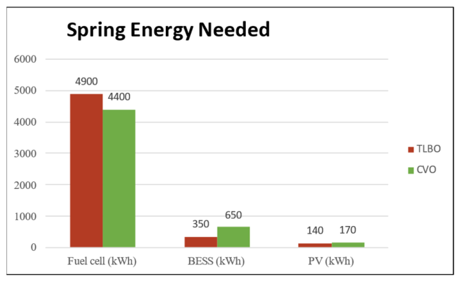
In spring, PV production and WASP contribution are lower than during summer, leading to higher reliance on the fuel cell. Figure 5 shows that the energy provided by the fuel cell is approximately 4900 kWh using the TLBO and 4400 kWh using the CVO. The PV produced energy is 140 kWh in TLBO and 170 kWh in CVO.

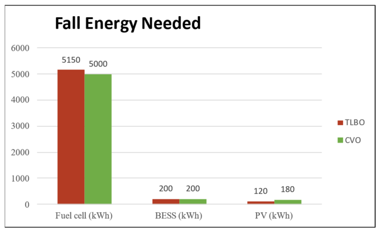
In fall, the required energy from the fuel cell is further increased. Figure 6 shows that the energy provided by the fuel cell is approximately 5150 kWh using the TLBO and 5000 kWh using the CVO. The PV produced energy is 120 kWh in TLBO and 180 kWh in CVO.

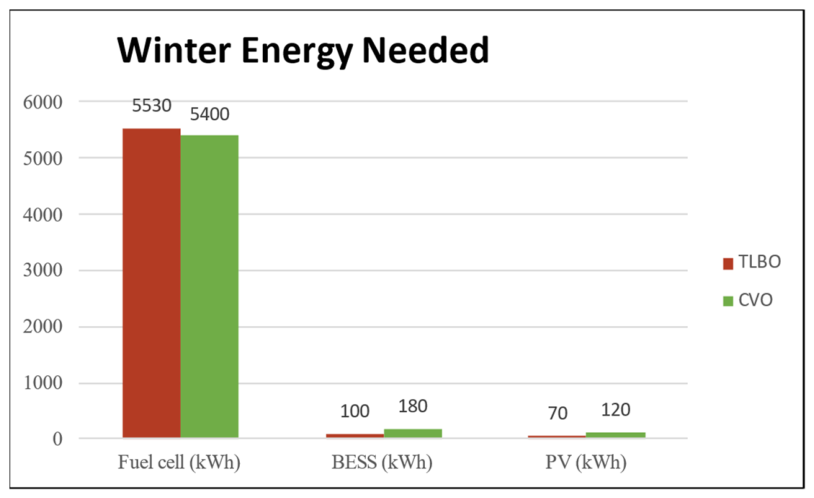
In winter, PV production and WASP contribution (less consistent winds) are the lowest of all the seasons, leading to the highest reliance on the fuel cell. Figure 7 shows that the energy provided by the fuel cell is approximately 5530 kWh using the TLBO and 5400 kWh using the CVO. The PV produced energy is 70 kWh in TLBO and 120 kWh in CVO.

Overall, in summer the high contribution from solar and wind energy significantly reduces the fuel cell’s production and hydrogen usage. In winter, the system relies highly on the fuel cell due to minimal solar and wind contributions. In all seasons, the CVO leads to lower fuel cell production and lower PV curtailment than the TLBO. On the other hand, the CVO leads to higher BESS contribution, which results in higher battery degradation than the TLBO. Additional analysis for the seasonal variations is included in Section 4.2.

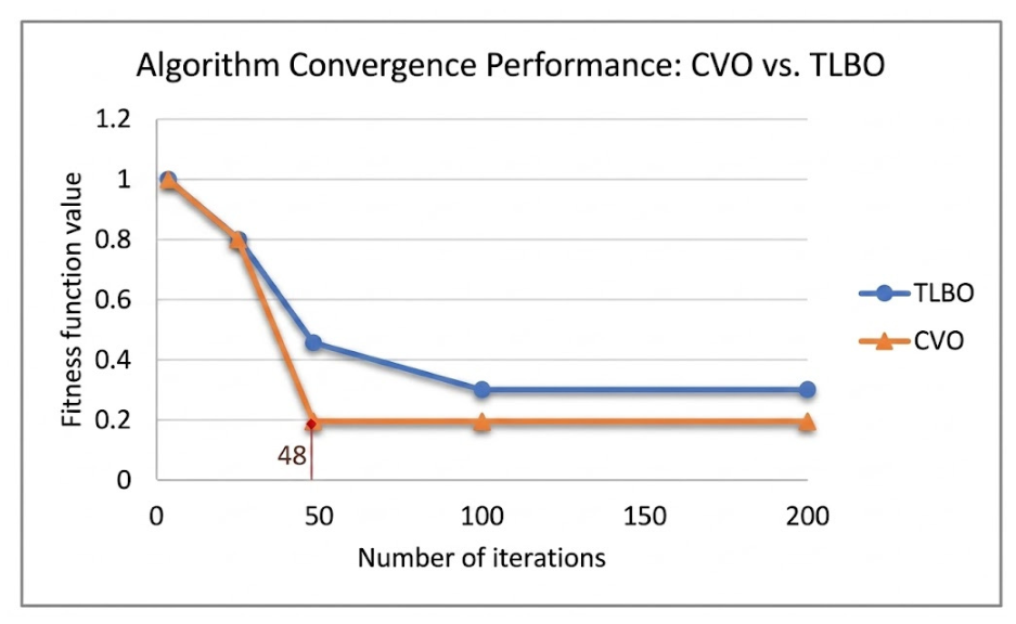
Figure 8 shows a comparison of the convergence performance between the CVO and TLBO. CVO performs better than TLBO in reaching the best solution (global maximum or minimum) with less computational time and iterations. CVO has better probability than TLBO in reaching global maximum or minimum than local ones.

4. Real-Time Dynamic Simulations

4.1. Modeling

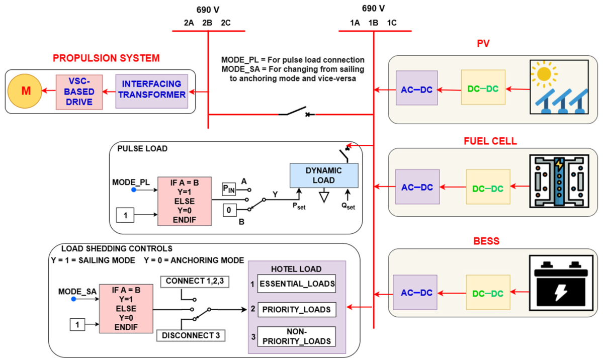
Real-time electromagnetic transient (EMT) simulations [50,51] were carried out in RSCAD(FX 2.6)/RTDS to analyze the operation of the proposed hybrid ship microgrid at four indicative seasonal scenarios, as well as during rapid load changes. The microgrid nominal values presented in Section 2 for the fuel cell, BESS, PVs and load are used. The single line diagram of the low voltage AC microgrid developed in RSCAD/RTDS is shown in Figure 9. Full PWM switching models were used for the converters of the fuel cell, BESS, PVs and propulsion drive, along with detailed models of the primary sources (fuel cell, batteries, PV) and propulsion motor.

The fuel cell model employed in this work is formulated primarily from steady-state electrochemical and mass-balance relations. Its implementation within the RTDS/RSCAD environment inherently captures the dynamic behavior relevant to shipboard power system studies. In particular, the RSCAD-based representation incorporates auxiliary balance-of-plant subsystems, including the DC/DC and DC/AC interfacing converter, fuel-flow regulation, air supply management, cooling control, and water/humidity regulation associated with practical stack operation. The model consists of fuel-cell stacks supplied through a common hydrogen storage system, with coordinated control signals scaled to satisfy the aggregate flow. These control and thermal-management subsystems govern the effective dynamic power exchange between the fuel cell and the point of common coupling during millisecond-scale electromagnetic disturbances, while also emulating the slower thermo-fluid dynamics influencing stack temperature, membrane hydration, hydrogen utilization, and electrochemical performance. Owing to the comparatively slower electrochemical and gas diffusion dynamics of fuel cells relative to converter switching phenomena, the adopted model is considered appropriate for such system-level EMT analysis. Similarly, PVs and BESS are modeled in RSCAD via well-known dynamic models.

The BESS converter acts as the grid-forming (GFM) converter, creating the microgrid voltage and frequency, while the fuel cell and PV converters are grid-following (GFL) units. The BESS, as the GFM unit, is responsible for maintaining the microgrid power balance. The vessel loads comprise the propulsion system and the hotel load. The hotel load is further classified into essential, priority, and non-priority categories. The operating mode of the vessel determines the load connection status. Figure 9 shows the load shedding control scheme. During sailing mode, all hotel loads remain connected, whereas in anchoring mode, only the essential and priority loads remain connected, with the non-priority loads being disconnected. Overall, a simulation time-step of 50 µs was used for the power system execution and smaller time-step for the converter switching.

4.2. Seasonal Variation

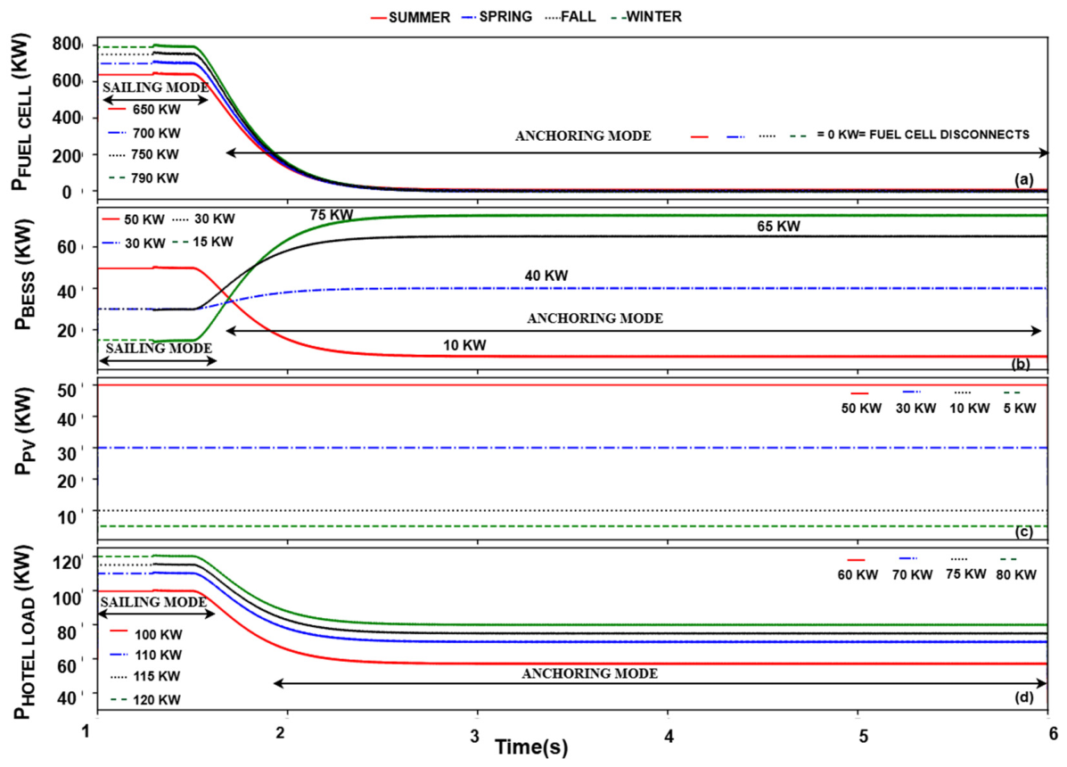
The transition between sailing and anchoring mode is analyzed with dynamic simulations for indicative seasonal profiles. The active power of the fuel cell, BESS, PV and hotel load during a 6 s time interval is presented in Figure 10.

During sailing mode, the major part of the total load (propulsion and hotel load) is supplied by the fuel cell, according to the EMS. This is supplemented by active power production of the BESS and PVs, while WASP reduces the propulsion load. Winter and summer are discussed below as the extreme cases, while spring and fall lie in between. During winter, the propulsion load is higher due to less contribution of the WASP because of less consistent and more stormy winds in the Aegean Sea. In addition, the power production of the PVs is the lowest during winter (Figure 10c). These two reasons raise the need for higher production of the fuel cell during winter (Figure 10a). On the other side, during summer the WASP makes use of the strong “Meltemi” wind, reducing the propulsion power, while the PV power is the highest (Figure 10c). Therefore, the active power supply of the fuel cell during summer is lower (Figure 10a).

During anchoring mode, obviously the propulsion system (and WASP) ceases to operate, while the hotel load is moderately reduced due to less utilization of HVAC and other loads (Figure 10d). According to the EMS, the fuel cell does not provide power during anchoring mode in all seasons (Figure 10a). Therefore, the hotel load is supplied by the BESS and the PVs. During winter, BESS supplies the major part of the hotel load (Figure 10b) due to limited PV production (Figure 10c). On the other side, during summer most of the hotel load is supplied by the PVs (Figure 10c), supported by the BESS (Figure 10b).

The transitions from sailing to anchoring mode reflect these observations. The fuel cell ceases to deliver active power (Figure 10a). The active power of the BESS is increased in order to supply the major part of the hotel load, apart from the summer case, where the high PV production leads to reduction in the BESS power (Figure 10b). The PV production remains unchanged during the transition in these scenarios (Figure 10c), while the hotel load is reduced, as already discussed (Figure 10d).

4.3. Rapid Load Increase and Wind Speed Variation

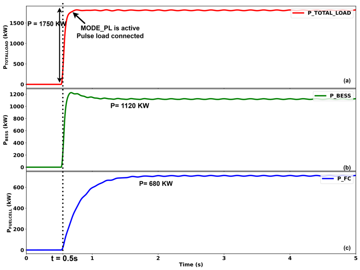
A worst-case dynamic scenario is considered to test the dynamic response of the system: maneuvering using bow thrusters [52] and rapid power increase in the propulsion motor in overloaded conditions for a few seconds. Figure 11 shows the rapid power increase in the total load. In response the active power of BESS increases quickly. The fuel cell active power also increases, but its reaction is slower than the BESS due to the inherent dynamics of the fuel cell system. During the transient, as the active power of the fuel cell increases, the active power of the BESS decreases. Overall, the load increase is shared among the fuel cell and the BESS. From an operational perspective, the BESS converter acts as the GFM converter, creating the microgrid voltage and frequency, while the fuel cell converter is a GFL device. During the load increase the BESS, as the GFM unit, naturally increases its active power in order to maintain the power balance. The fuel cell as a GFL unit (without droop control in this analysis) needs to receive a command to increase its active power. Therefore, it receives a setpoint from the operator, simultaneously with the planned rapid load increase, in order to increase its output.

The rapid load increase may impose significant thermal stresses on fuel cells, potentially influencing their temperature-dependent state-of-health (SOH) degradation characteristics. Recent studies have emphasized the importance of adaptive thermal and SOH-aware management strategies to enhance PEMFC durability and operational reliability under dynamic operating conditions [53].

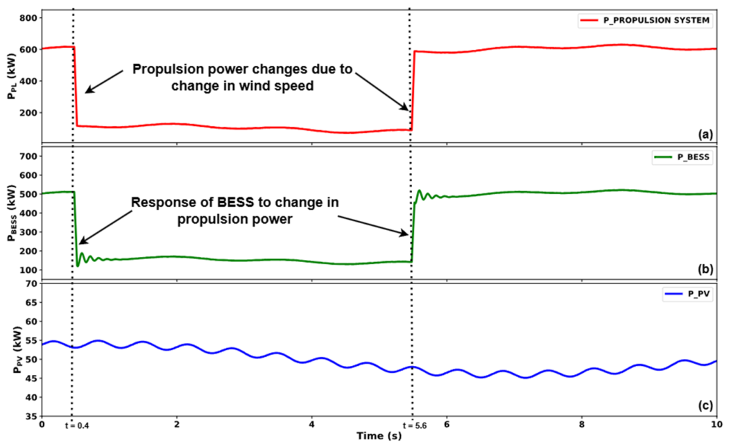
The electric propulsion power is affected by the WASP contribution, which depends on the wind speed. Figure 12 shows dynamic simulation results during an abrupt change in WASP contribution due to extreme wind speed variation. The wind speed is highly increased, leading to a significant increase in the WASP contribution and thus to a reduction in the active power of the propulsion system. Accordingly, the BESS reduces its active power as the GFM unit responsible for maintaining power balance. Next, the wind speed is abruptly and significantly reduced, leading to an increase in the active power of the propulsion system and BESS. The PV active power variation depends on the solar irradiation.

5. Converter-Driven Stability

As explained in the introduction, converter-driven stability has been recognized as an emerging power system stability issue and has been added as a new category in the recent stability classification of IEEE [35,36]. High-frequency oscillations, classified as fast-interaction converter-driven stability in [35,36], can rise from the interaction between the fast current controllers of converters connected at close proximity [37]. These types of phenomena have been mainly witnessed in terrestrial transmission and distribution systems, but they could also be potentially triggered in modern and future shipboard microgrids due to the high penetration of power electronic devices (e.g., converters of fuel cells, BESS, PVs, propulsion drives, HVAC systems, etc.).

5.1. Impedance-Based Analysis: Modeling

In recent years, impedance-based stability analysis, requiring linear time invariant modeling of each system component, has been widely used for stability studies in power systems. Linear models for both grid-following (GFL) and grid-forming (GFM) control schemes in ab frame have been developed in [54] and used in [40] for the investigation of fast interaction converter-driven stability phenomena in microgrids.

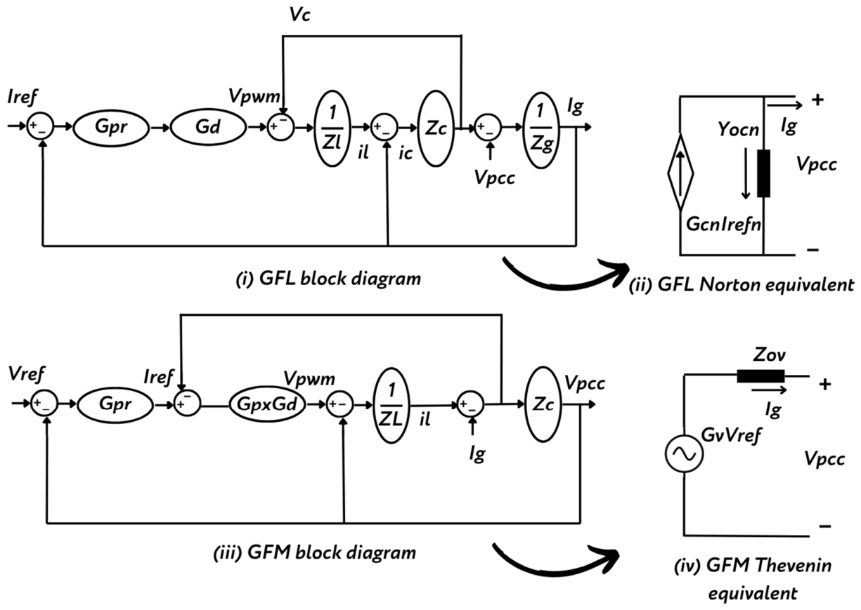
By assuming that the phase-locked loop (PLL) mechanism of the GFL inverter is perfectly locked, the grid is symmetrical, and by neglecting the dynamics of inverter switching devices, the following set of equations have been extracted, representing the current control, the computational delay and the LCL filter dynamics. The block diagram of the GFL inverter is presented in Figure 13i. The current control is implemented with a PR controller with transfer function:

$$G_{pri}=k_{pi}+{\displaystyle \frac{k_{ii}·s}{s^2+{\omega }_1^2}}$$

(32)

where $k_{pi}$ is the proportional gain, $k_{ii}$ is the integral gain and ${\omega }_1$ is the nominal angular velocity of the grid.

Computational delay, rising from measurement, communication, processing, the PWM technique, etc., is modeled as follows:

$$G_d=e^{-1.5·T_s·s}$$

(33)

where Ts is the sampling time of the system. An LCL filter is used for harmonic mitigation. $I_{ref}$ is the current reference of the current controller, $I_g$ is the output current of the inverter, $V_{pwm}$ is the output voltage of the inverter, $V_c$ is the voltage of the capacitor, $V_{pcc}$ is the voltage at the point of connection, $i_c$ is the current of the capacitor, $i_l$ is the current of the l inductance,

$$z_l=R_l+s·X_l$$

(34)

is the impedance of the l inductance,

$$z_g=R_g+s·X_g$$

(35)

is the impedance of the g inductance and

$$Z_C={\displaystyle \frac{1}{s·C}}$$

(36)

is the admittance of the capacitor.

The voltage of the PWM technique $V_{pwm}$, the current of the l inductor $i_l$, the current of the C capacitor $i_c$ and the output current of the inverter $I_g$ are calculated based on Kirchhoff laws with the following equations:

$$(I_{ref}-I_g)·G_{pr}·G_d=V_{pwm},\hspace{1em}(V_{pwm}-V_c)·{\displaystyle \frac{1}{z_L}}=i_l$$

(37)

$$i_l-I_g=i_c={\displaystyle \frac{V_C}{Z_C}},\hspace{1em}\left(V_c-V_{pcc}\right){\displaystyle \raisebox{1ex}{$1$}\!\left/ \!\raisebox{-1ex}{$z_g$}\right.}=I_g(\mathbf{2})$$

(38)

Using this set of equations, a GFL inverter in the frequency domain can be represented as a current source with dynamic gain ${\mathrm{G}}_{\mathrm{c}}$ in parallel with an $Y_{oc}$ admittance (Norton Equivalent), as presented in Figure 13ii:

$$Y_{oc}(I_{ref}=0)={\displaystyle \frac{I_g}{V_{pcc}}}={\displaystyle \frac{Z_c+Z_L}{Z_L·Z_c+Z_c·Z_g+Z_g·Z_L+G_{pr}·G_d·Z_c}}$$

(39)

$$G_c(V_{pcc}=0)={\displaystyle \frac{I_g}{I_{ref}}}={\displaystyle \frac{G_{pr}\mathrm{\ast }{G}_d\mathrm{\ast }{Z}_c}{Z_L·Z_c+Z_c·Z_g+Z_g·Z_L+G_{pr}·G_d·Z_c}}$$

(40)

Similarly, by neglecting the dynamics of inverter switching devices, the following set of equations representing the voltage control, current control, computational delay and LC filter dynamics is extracted along with the block diagram of a GFM inverter (Figure 13iii). The voltage control is implemented with a PR controller with transfer function:

$$G_{prv}=k_{pv}+{\displaystyle \frac{k_{iv}·s}{s^2+{\omega }_1^2}}$$

(41)

where $k_{pv}$ is the proportional gain, $k_{iv}$ is the integral gain and ${\omega }_1$ is the nominal angular velocity of the grid. The current control receives its reference from the output of the voltage controller and is implemented with a proportional-P controller with transfer function:

$$G_p=k_{pvi}$$

(42)

where $k_{pvi}$ is the proportional gain. The computational delay rising from the telecommunication devices and the PWM technique is modeled as $G_d=e^{-1.5T_{s}s},$ whereas Ts is the sampling time of the system. An LC filter is used for harmonic mitigation. $V_{ref}$ is the voltage reference of the voltage controller, $I_{ref}$ is the current reference of the current controller, $I_g$ is the output current of the inverter, $V_{pwm}$ is the output voltage of the inverter, $V_c$ is the voltage of the capacitor, $V_{pcc} \mathrm{i}\mathrm{s} \mathrm{t}\mathrm{h}\mathrm{e} \mathrm{v}\mathrm{o}\mathrm{l}\mathrm{t}\mathrm{a}\mathrm{g}\mathrm{e} \mathrm{a}\mathrm{t} \mathrm{t}\mathrm{h}\mathrm{e} \mathrm{p}\mathrm{o}\mathrm{i}\mathrm{n}\mathrm{t} \mathrm{o}\mathrm{f} \mathrm{c}\mathrm{o}\mathrm{n}\mathrm{n}\mathrm{e}\mathrm{c}\mathrm{t}\mathrm{i}\mathrm{o}\mathrm{n},$ $i_c$ is the current of the capacitor and $i_l$ is the current of the inductance.

$$z_L=R_L+s·X_L$$

(43)

is the impedance of the L inductance, and

$$Z_C={\displaystyle \frac{1}{s·C}}$$

(44)

is the impedance of the capacitor.

The current reference $I_{ref}$, the voltage of the PWM technique $V_{pwm}$, the current of the L inductor $i_L$ and the output current of the inverter $I_g$ are calculated based on Kirchhoff laws with the following equations:

$$(V_{ref}-V_c)·G_{pr}=I_{ref}$$

(45)

$$(I_{ref}-i_L)·G_p·G_d=V_{pwm}$$

(46)

$$\left(V_{pwm}-V_c\right){\displaystyle \raisebox{1ex}{$1$}\!\left/ \!\raisebox{-1ex}{$z_L$}\right.}=i_L$$

(47)

$$I_g=-{\displaystyle \frac{V_C}{Z_C}}+i_L$$

(48)

Using this set of equations, the GFM inverter in the frequency domain can be represented as a voltage source with dynamic gain $G_v$ in series with an $Z_{ov}$ impedance (Thevenin Equivalent), as presented in Figure 13iv:

$$Z_{ov}\left(V_{ref}=0\right)={\displaystyle \frac{V_{pcc}}{I_g}}={\displaystyle \frac{Z_C\left(G_d·G_p+Z_L\right)}{Z_L+Z_c+G_{pr}·G_p·G_d+G_p·G_d}}$$

(49)

$$G_v\left(I_g=0\right)={\displaystyle \frac{V_{pcc}}{V_{ref}}}={\displaystyle \frac{Z_C(G_d·G_p·G_{pr})}{Z_L+Z_c+G_{pr}·G_p·G_d+G_p·G_d}}$$

(50)

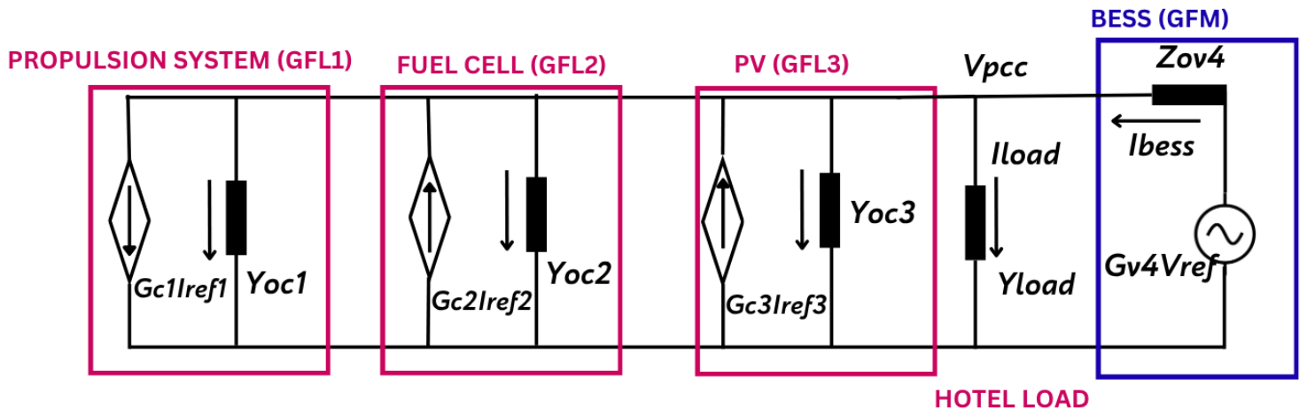
The considered topology for the fast-interaction converter-driven stability analysis of the shipboard microgrid is shown in Figure 14. The microgrid data presented in Section 2 for the fuel cell, BESS, PVs and load are used. A low voltage AC microgrid is considered where the BESS inverter operates as the GFM converter, which takes over the creation of the voltage and frequency of the microgrid. The fuel cell and the PV inverters operate as GFL converters. The propulsion system consists of AC/DC and DC/AC converters and a propulsion motor. An active-front end is employed for the rectifier of the propulsion drive, as an emerging technology for propulsion drives, especially for passenger ferries [55]. Therefore, from a microgrid perspective, the propulsion drive is considered as a GFL converter.

In order to study fast-interaction converter-driven stability in the considered topology, the GFL converters of the propulsion system, fuel cell and PVs have been represented with their Norton equivalent of Figure 13ii, and the GFM inverter of BESS has been represented with its Thevenin equivalent of Figure 13iv, as illustrated in Figure 14. It is worth noting that GFL2 (fuel cell) and GFL3 inverters (PV) inject active power to the microgrid, thus their current sources $I_{ref2},I_{ref3}$ have positive signs, while the GFL1 converter (propulsion system) absorbs active power, thus its current source $I_{ref1}$ has a negative sign. By applying the superposition theorem, the voltage at the point of connection $V_{pcc}$ is extracted, as follows.

$$V_{pcc}=V_{ref}·{\displaystyle \frac{G_v}{1+F\left(s\right)}}+I_{ref1}·{\displaystyle \frac{G_{c1}·Z_{ov}}{1+F\left(s\right)}}+I_{ref2}·{\displaystyle \frac{G_{c2}·Z_{ov}}{1+F\left(s\right)}}-I_{ref3}·{\displaystyle \frac{G_{c3}·Z_{ov}}{1+F\left(s\right)}}$$

(51)

$$V_{pcc}={\displaystyle \frac{1}{1+F\left(s\right)}}(V_{ref}·G_v+I_{ref1}·G_{c1}\ast Z_{ov}+I_{ref2}·G_{c2}·Z_{ov}-I_{ref3}·G_{c3}·Z_{ov})$$

(52)

where

$$F\left(s\right)=Z_{ov4}·Y_{oc1}+Z_{ov4}·Y_{oc2}{+Z_{ov4}·Y_{oc3}+Z}_{ov4}·Y_{load}$$

(53)

$Y_{oc1}$, $Y_{oc2}$, and $Y_{oc3}$ are the output admittances of the three GFL converters (active-front end of propulsion system, fuel cell, and PVs, respectively), while $G_{c1}$, $G_{c2}$ and $G_{c3}$ model the dynamic performance of the three GFL converters, as explained above

$Z_{ov4}$ is the output impedance of the GFM converter (BESS), while $G_v$ models its dynamic performance, as explained above.

$Y_{load}$ models the admittance of the non-power electronic load.

$I_{ref1}$, $I_{ref2}$ and $I_{ref3}$ are the reference values of the output current of the three GFL converters, while $V_{ref}$ is the reference value of the output voltage of the GFM converter.

According to control system theory for linear time invariant systems, the voltage at the point of connection ($V_{pcc})$ is stable if it does not have any poles in the right half plane [56,57,58]. The current and voltage reference sources $I_{ref}$ and $V_{ref}$ are stable sinusoidal signals, and $G_v,$ $Z_{ov},G_{c1},G_{c2},G_{c3}$ transfer functions associated with the converters do not have any poles in the right half plane. Thus, the fast-interaction converter-driven stability of the system can be assessed by tracking the location of the poles of the ${\displaystyle \frac{1}{1+F\left(s\right)}}$ transfer function, which correspond to the zeros of systems characteristic polynomial equation $1+F\left(s\right)$, which is a polynomial function of the 41st grade.

5.2. Impedance-Based Analysis: Results

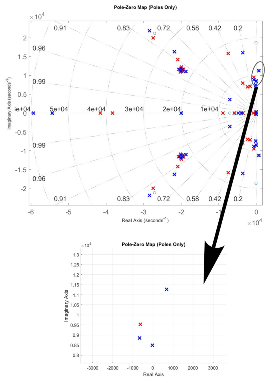
For the initial control and filter parameters of the converters shown in

Table 1. Control parameters (initial and maximum values) and filters of the converters

Converter Parameters	Values
GFL1 Parameters (Propulsion System)
Current controller (PR1):
Kp_1	Initial value = 0.5 Max value = 1.05
Ki_1	50
LCL filter:
Ll1 C1	10 μH, resistive part: 0.01 Ω 20 μF, resistive part: 0.5 Ω
Lg1	10 μH, resistive part: 0.01 Ω
GFL2 Parameters (Fuel Cell)
Current controller (PR2):
Kp_2	Initial value = 0.5 Max value = 0.7
Ki_2	50
LCL filter:
Ll2 C2	5 μH, resistive part: 0.01 Ω 40 μF, resistive part: 0.5 Ω
Lg2	5 μH, resistive part: 0.01 Ω
GFL3 Parameters (PV)
Current controller (PR3)
Kp_3	Initial value = 1 Max value = 3.6
Ki_3	50
LCL filter
Ll3 C3	80 μH, resistive part: 0.01 Ω 3 μF, resistive part: 0.5 Ω
Lg3	80 μH, resistive part: 0.01 Ω
GFM Parameters (BESS)
Voltage Controller (PR4)
Kp_v_4	0.2
Ki_v_4	10
Current controller (P)
Kp_i4	Initial value = 0.2 Max value = 0.5
LC filter
LL4 C4	40 μH, resistive part: 0.02 Ω 100 μF, resistive part: 0.5 Ω

and the system parameters presented in

Table 2. System parameters.

System	Values
Base voltage (Vb)	690 V
Base power	100 MVA
Nominal frequency	50 Hz
Hotel load (operating condition)	100 kW
Propulsion system (operating condition)	637.5 kW
BESS (operating condition)	50 kW
PV (operating condition)	37.5 kW
Fuel Cell (operating condition)	650 kW

, the systems’ poles are extracted and presented in the pole-zero map of Figure 15 in red color. It can be seen that all the poles have negative real parts, therefore the system is stable. By applying participation factor analysis, the mode with frequency 1520 Hz (9550 r/s) has damping of 0.0656, which is closer to zero than all the other modes. Next, the proportional gains of all the current controllers are increased to their maximum values (shown in Table 1), and the poles of the system are marked with blue color in Figure 15. In this case, there is one set of high-frequency poles at 1799 Hz (11,300 r/s), situated in the right half plane of the pole-zero map, indicating that the critical pole has moved in the right half plane, and the system is now unstable.

An interpretation of the results follows. Naturally, each individual converter is stable when its current controller operates with its maximum allowable proportional gain. However, when all the converters were operating simultaneously with their maximum proportional gains, within the shipboard microgrid, the system became unstable due to the interactions among the converters. This highlights the practical value and need for further investigation of fast-interaction converter-driven stability of shipboard microgrids.

5.3. Time Domain Simulations: Modeling and Results

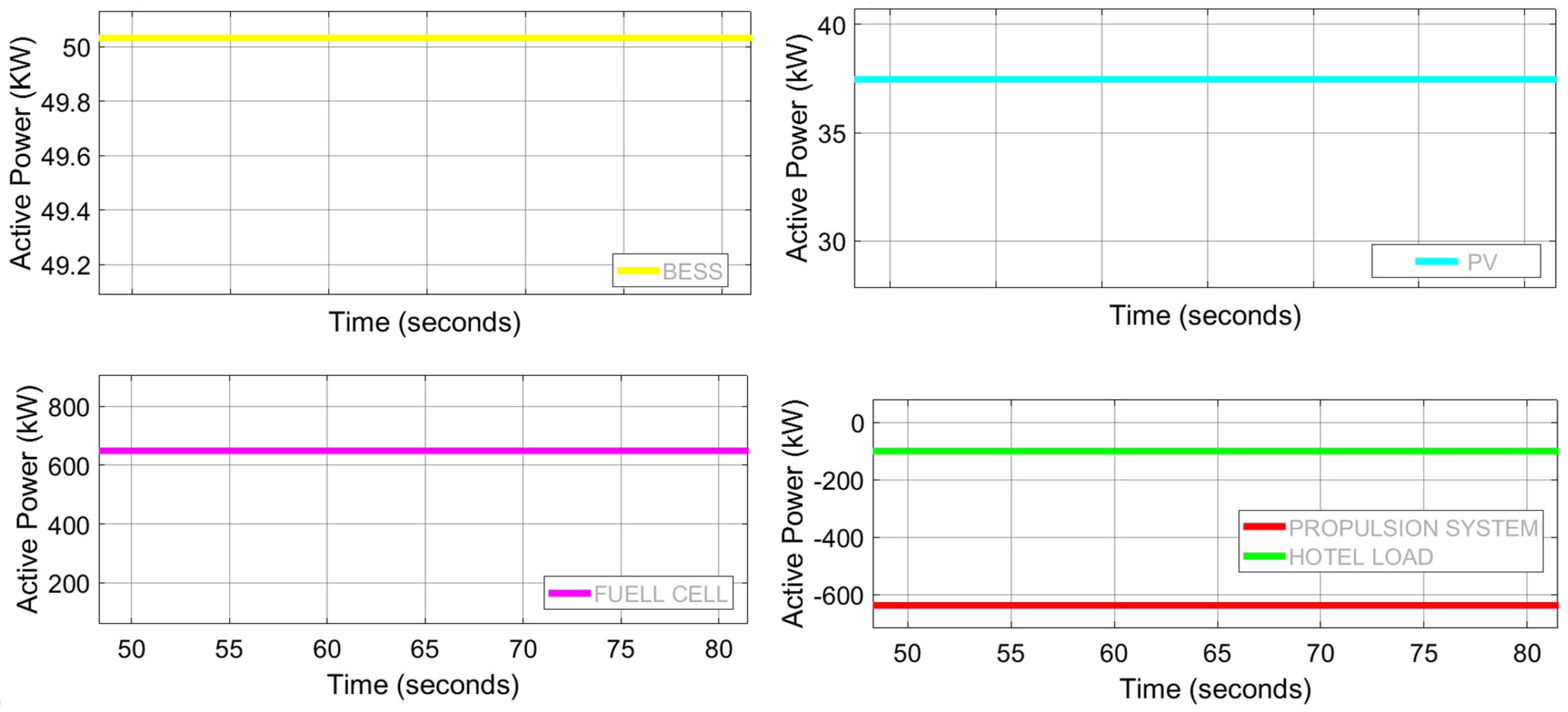
A time-domain simulation of the shipboard microgrid was built in Matlab 2018b/Simulink environment for the validation of the theoretical results of the impedance-based analysis. Average models of the different converters were developed within the shipboard microgrid. The GFM and GFL configuration explained in Section 5.1 was applied, along with the controller parameters of Table 1. First, the initial controller parameters (Table 1) were applied, and the active power of the BESS, fuel cell, PV, propulsion system and hotel load are presented in Figure 16, showing stable operating conditions. The specific operating conditions illustrated in Figure 16 are included in Table 2.

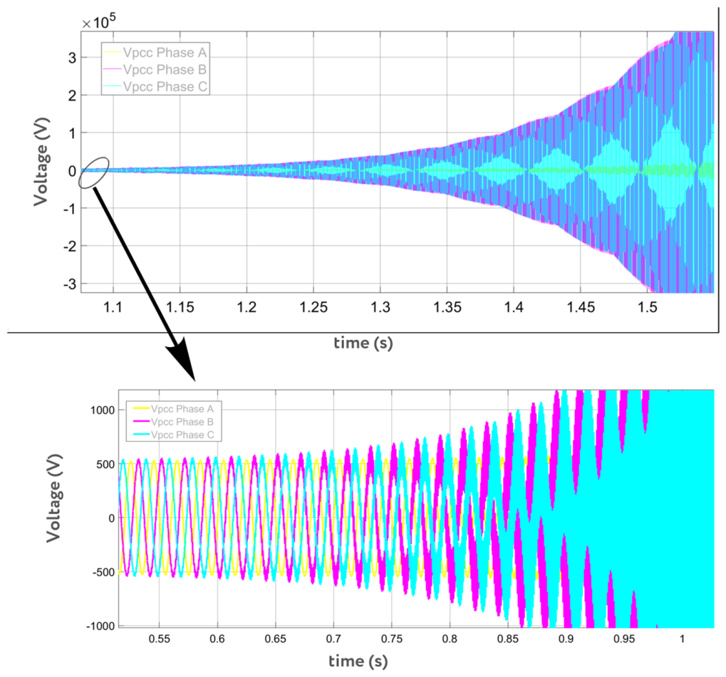
Next, the proportional gains of all the current controllers were increased to the maximum values (Table 1). Figure 17 shows that the voltage at the point of connection increases quickly from amplitude of V_pcc = (V_b$·\sqrt{2})$/$\sqrt{3}$ to very high values of MV, demonstrating instability. The time-domain simulation results match the results of the impedance-based analysis, validating the accuracy of the analysis.

6. Conclusions

This paper addressed the operation of a zero-emission electric passenger ferry powered by fuel cell, BESS, and PVs, and supported by WASP under the environmental conditions of the Aegean Sea, Greece. The hypothetical microgrid is rich in renewable energy resources, in order to reduce the reliance on fuel cell hydrogen. A complete analysis was performed, which included optimal energy management, dynamic simulations and converter-driven stability.

Concerning the EMS operation, the results highlight clear seasonal trends. Higher PV production and WASP contribution in summer reduced fuel cell loading and hydrogen usage. On the other hand, in winter the system relied more on the fuel cell due to limited solar and wind contributions. Overall, the combination of WASP and PVs was beneficial for enhancing the overall efficiency and reducing hydrogen consumption, making the system more environmentally sustainable. Concerning the two optimization algorithms applied, the CVO resulted in lower fuel cell production and lower PV curtailment than the TLBO in all seasons. On the other hand, the CVO led to higher BESS contribution, resulting in higher battery degradation than the TLBO.

The real-time dynamic simulations further analyzed the operation of the shipboard microgrid. The transition from sailing mode to anchoring mode was examined, providing additional insights on the operation of the system at the different seasons. Moreover, the coordination among the BESS (GFM converter) and the fuel cell (GFL converter) during a rapid load increase was examined, highlighting the faster response of the BESS. Significant changes in WASP contribution were also simulated

Fast-interaction converter-driven stability issues were investigated, which may arise due to interactions among the various converter controllers and passive components of the microgrid. Both impedance-based analysis and time domain simulations were employed in order to substantiate the approach, revealing the same results. When all the converters were operating simultaneously with their maximum allowable proportional gains, the shipboard microgrid became unstable due to the interactions among the converters. This highlights the need for further investigation of fast-interaction converter-driven stability of shipboard microgrids.

Concerning future work, it is suggested to address the uncertainty of solar and wind contributions in the EMS operation of zero-emission vessels. Fast-interaction converter-driven stability for shipboard microgrids will be further investigated, since this promising area has not been sufficiently explored yet.

References

1. International Maritime Organization. 2023 IMO Strategy on Reduction of Greenhouse Gas Emissions from Ships; International Maritime Organization: London, UK, 2023. [Google Scholar]
2. Li, X.; Ye, T.; Meng, X.; He, D.; Li, L.; Song, K.; Jiang, J.; Sun, C. Advances in the Application of Sulfonated Poly(Ether Ether Ketone) (SPEEK) and Its Organic Composite Membranes for Proton Exchange Membrane Fuel Cells (PEMFCs). Polymers 2024, 16, 2840. [Google Scholar] [CrossRef]
3. Coraddu, A.; Tamburello, S.; Löffler, C.; Ceyhun, H.E.; van Biert, L.; Oneto, L. State-of-art energy management strategies for hybrid fuel cell applications for ships. In Fuel Cell and Hydrogen Technologies in Maritime Transportation; Springer Nature: Cham, Switzerland, 2025. [Google Scholar]
4. Khan, A.A.; Timilsina, L.; Muriithi, G.; Arsalan, A.; Moghassemi, A.; Papari, B.; Ozkan, G.; Edrington, C.S.; Boghrabadi, N.S.; Wang, Z. Energy Management Systems for Maritime Microgrids: A Comprehensive Review of Intelligent Optimization Strategies. IEEE Access 2025, 13, 171563–171597. [Google Scholar] [CrossRef]
5. Sarkar, M.R.; Park, Y.; Park, H.; Woo, J.; Son, H. Hybrid Energy Storage Systems, Converter Topologies, Energy Management Systems, and Future Prospects of Green Marine Technology: A Comprehensive Review. IEEE Access 2025, 13, 54592–54638. [Google Scholar] [CrossRef]
6. Bai, M.; Ke, W.; Wu, C.; Cheng, H.; Zhang, J.; Yang, X. Energy Management Strategies for Fuel Cell Hybrid Ships: Classification, Comparison, and Outlook. Energies 2026, 19, 1171. [Google Scholar] [CrossRef]
7. Tian, C.; Zhang, L.; Zou, L.; Liu, X. Research progress on topology and energy management of fuel cell hybrid power ships. J. Phys. Conf. Ser. 2024, 2876, 042092. [Google Scholar] [CrossRef]
8. Xie, P.; Guerrero, J.M.; Tan, S.; Bazmohammadi, N.; Vasquez, J.C.; Mehrzadi, M.; Al-Turki, Y. Optimization-based power and energy management system in shipboard microgrid: A review. IEEE Syst. J. 2021, 16, 578–593. [Google Scholar] [CrossRef]
9. Rafiei, M.; Boudjadar, J.; Khooban, M.H. Energy management of a zero-emission ferry boat with a fuel-cell-based hybrid energy system: Feasibility assessment. IEEE Trans. Ind. Electron. 2020, 68, 1739–1748. [Google Scholar] [CrossRef]
10. Peng, X.; Chen, H.; Guan, C. Energy Management Optimization of Fuel Cell Hybrid Ship Based on Particle Swarm Optimization Algorithm. Energies 2023, 16, 1373. [Google Scholar] [CrossRef]
11. Zhang, Z.; Guan, C.; Liu, Z. Real-time optimization energy management strategy for fuel cell hybrid ships considering power sources degradation. IEEE Access 2020, 8, 87046–87059. [Google Scholar] [CrossRef]
12. Qu, J.; Wang, H.; Zou, L.; Zhang, L.; Zhang, T.; Zhou, J.; Zhang, B. A two-layer energy management strategy of fuel cell hybrid system in electric ships. IEEE Trans. Ind. Appl. 2024, 61, 3622–3634. [Google Scholar] [CrossRef]
13. Kamilakis, E.; Pourakbari-Kasmaei, M.; Kotsampopoulos, P.; Rigmor Nerheim, A. Multi-Objective Energy Management of PEMFC Maritime Power Systems: Balancing Fuel Use and Load-Induced Degradation. In Proceedings of the Accepted for Presentation at ASME 2026 45th International Conference on Ocean, Offshore and Arctic Engineering, OMAE2026, Tokyo, Japan, 7–12 June 2026. [Google Scholar]
14. Nivolianiti, E.; Karnavas, Y.L.; Charpentier, J.-F. Fuzzy Logic-Based Energy Management Strategy for Hybrid Fuel Cell Electric Ship Power and Propulsion System. J. Mar. Sci. Eng. 2024, 12, 1813. [Google Scholar] [CrossRef]
15. Manickavasagam, K.; Thotakanama, N.K.; Puttaraj, V. Intelligent energy management system for renewable energy driven ship. IET Electr. Syst. Transp. 2019, 9, 15–24. [Google Scholar] [CrossRef]
16. Zhao, Z.H. Improved fuzzy logic control-based energy management strategy for hybrid power system of FC/PV/battery/SC on tourist ship. Int. J. Hydrogen Energy 2022, 47, 0003–10018. [Google Scholar] [CrossRef]
17. Xie, P.; Asgharian, H.; Guerrero, J.M.; Vasquez, J.C.; Araya, S.S.; Liso, V. A two-layer energy management system for a hybrid electrical passenger ship with multi-PEM fuel cell stack. Int. J. Hydrogen Energy 2024, 50, 1391–1405. [Google Scholar] [CrossRef]
18. Accetta, A.; Pucci, M. Energy management system in DC micro-grids of smart ships: Main gen-set fuel consumption minimization and fault compensation. IEEE Trans. Industry Appl. 2019, 55, 3097–3113. [Google Scholar] [CrossRef]
19. Jamma, M.; Bujlo, P.; Ulleberg, Ø. Intelligent energy management system for hybrid fuel cell/battery powered ships. IEEE Trans. Ind. Appl. 2025, 61, 8283–8296. [Google Scholar] [CrossRef]
20. Wu, P.; Partridge, J.; Bucknall, R. Cost-effective reinforcement learning energy management for plug-in hybrid fuel cell and battery ships. Appl. Energy 2020, 275, 115258. [Google Scholar] [CrossRef]
21. Zhu, L.; Liu, Y.; Zeng, Y.; Guo, H.; Ma, K.; Liu, S.; Zhang, Q. Energy management strategy for fuel cell hybrid ships based on deep reinforcement learning with multi-optimization objectives. Int. J. Hydrogen Energy 2024, 93, 1117–1132. [Google Scholar] [CrossRef]
22. Liu, L.; Yang, X.; Li, X.; Zhou, X.; Wang, Y.; Tang, T.; Song, Q.; Liu, Y. Prior Knowledge-Based Two-Layer Energy Management Strategy for Fuel Cell Ship Hybrid Power System. J. Mar. Sci. Eng. 2025, 13, 94. [Google Scholar] [CrossRef]
23. Chen, W.; Tai, K.; Lau, M.W.S.; Abdelhakim, A.; Chan, R.R.; Ådnanes, A.K.; Tjahjowidodo, T. Optimal power and energy management control for hybrid fuel cell-fed shipboard DC microgrid. IEEE Trans. Intell. Transp. Syst. 2023, 24, 14437–14450. [Google Scholar] [CrossRef]
24. Martínez-Álvarez, F.; Asencio-Cortés, G.; Torres, J.F.; Gutiérrez-Avilés, D.; Melgar-García, L.; Pérez-Chacón, R.; Rubio-Escudero, C.; Riquelme, J.C.; Troncoso, A. Coronavirus Optimization Algorithm: A bioinspired metaheuristic based on the COVID-19 propagation model. Big Data 2020, 8, 308–322. [Google Scholar] [CrossRef]
25. Salehan, A.; Deldari, A. Corona virus optimization (CVO): A novel optimization algorithm inspired from the Corona virus pandemic. J. Supercomput. 2022, 78, 4975–5006. [Google Scholar] [CrossRef] [PubMed]
26. Fayek, H.H.; Abdalla, O.H. Operation of the Egyptian Power Grid with Maximum Penetration Level of Renewable Energies Using Corona Virus Optimization Algorithm. Smart Cities 2022, 5, 34–53. [Google Scholar] [CrossRef]
27. ALBaaj, B.; Kaplan, O. Enhanced COVID-19 Optimization Algorithm for Solving Multi-Objective Optimal Power Flow Problems with Uncertain Renewable Energy Sources: A Case Study of the Iraqi High-Voltage Grid. Energies 2025, 18, 478. [Google Scholar] [CrossRef]
28. ALbaaj, B.; Kaplan, O. Optimizing Energy Scheduling and Power Flow in the Power System Using Coronavirus Algorithm. In Proceedings of the 2024 6th Global Power, Energy and Communication Conference (GPECOM), Budapest, Hungary, 4–7 June 2024. [Google Scholar]
29. Safiullah, S.; Rahman, A.; Lone, S.A.; Hussain, S.M.S.; Ustun, T.S. Novel COVID-19 Based Optimization Algorithm (C-19BOA) for Performance Improvement of Power Systems. Sustainability 2022, 14, 14287. [Google Scholar] [CrossRef]
30. Rao, R.V.; Savsani, V.J.; Vakharia, D.P. Teaching-Learning Based Optimization: A Novel Optimization Method for Continuous Non-Linear Large Scale Problems. Inf. Sci. J. 2012, 183, 1–15. [Google Scholar] [CrossRef]
31. Fayek, H.H.; Abdalla, O.H. Maximization of Renewable Power Generation for Optimal Operation of the Egyptian Grid. In Proceedings of the 2020 IEEE 29th International Symposium on Industrial Electronics (ISIE), Delft, The Netherlands, 17–19 June 2020; pp. 1085–1090. [Google Scholar]
32. Sulaiman, M.H.; Mustaffa, Z.; Rashid, M.I.M. An application of teaching–learning-based optimization for solving the optimal power flow problem with stochastic wind and solar power generators. Results Control Optim. 2023, 10, 100194. [Google Scholar] [CrossRef]
33. Ermiş, S. Multi-objective optimal power flow using a modified weighted teaching-learning based optimization algorithm. Electr. Power Compon. Syst. 2023, 51, 2401–2417. [Google Scholar] [CrossRef]
34. Mei, J.; Meng, X.; Tang, X.; Li, H.; Hasanien, H.; Alharbi, M.; Dong, Z.; Shen, J.; Sun, C.; Fan, F.; et al. An Accurate Parameter Estimation Method of the Voltage Model for Proton Exchange Membrane Fuel Cells. Energies 2024, 17, 2917. [Google Scholar] [CrossRef]
35. Hatziargyriou, N.; Milanović, J.; Rahmann, C.; Ajjarapu, V.; Canizares, C.; Erlich, I.; Hill, D.; Hiskens, I.; Kamwa, I.; Pal, B.; et al. Stability Definitions and Characterization of Dynamic Behavior in Systems with High Penetration of Power Electronic Interfaced Technologies; IEEE PES Technical Report TR77; IEEE PES Resource Center: Piscataway, NJ, USA, 2020. [Google Scholar]
36. Hatziargyriou, N.; Milanovic, J.; Rahmann, C.; Ajjarapu, V.; Canizares, C.; Erlich, I.; Hill, D.; Hiskens, I.; Kamwa, I.; Pal, B.; et al. Definition and Classification of Power System Stability—Revisited & Extended. IEEE Trans. Power Syst. 2021, 36, 3271–3281. [Google Scholar]
37. Eckel, C.; Babazadeh, D.; Becker, C. Classification of Converter-Driven Stability and Suitable Modeling and Analysis Methods. IEEE Access 2024, 12, 111602–111627. [Google Scholar] [CrossRef]
38. Kong, L.; Xue, Y.; Qiao, L.; Wang, F. Review of small-signal converter-driven stability issues in power systems. IEEE Open Access J. Power Energy 2021, 9, 29–41. [Google Scholar] [CrossRef]
39. Luo, J.; Zou, Y.; Bu, S.; Karaagac, U. Converter-Driven Stability Analysis of Power Systems Integrated with Hybrid Renewable Energy Sources. Energies 2021, 14, 4290. [Google Scholar] [CrossRef]
40. Saridaki, G.; Paspatis, A.G.; Kotsampopoulos, P.; Hatziargyriou, N. An investigation of factors affecting Fast-Interaction Converter-driven stability in Microgrids. Electr. Power Syst. Res. 2023, 223, 109511. [Google Scholar] [CrossRef]
41. Bhandari, B.; Poudel, S.R.; Lee, K.T.; Ahn, S.H. Mathematical modeling of hybrid renewable energy system: A review on small hydro-solar-wind power generation. Int. J. Precis. Eng. Manuf.-Green Technol. 2014, 1, 157–173. [Google Scholar] [CrossRef]
42. Fayek, H.H.; Fayek, F.H.; Rusu, E. Quantum-Inspired MoE-Based Optimal Operation of a Wave Hydrogen Microgrid for Integrated Water, Hydrogen, and Electricity Supply and Trade. J. Mar. Sci. Eng. 2025, 13, 461. [Google Scholar] [CrossRef]
43. Meng, X.; Sun, C.; Mei, J.; Tang, X.; Hasanien, H.M.; Jiang, J.; Fan, F.; Song, K. Fuel cell life prediction considering the recovery phenomenon of reversible voltage loss. J. Power Sources 2025, 625, 235634. [Google Scholar] [CrossRef]
44. Li, H.; Sun, C.; Li, J.; Mei, J.; Jiang, J.; Fan, F.; Yang, W.; Zhuo, R.; Song, K. Self-Tuning Oxygen Excess Ratio Control for Proton Exchange Membrane Fuel Cells Under Dynamic Conditions. Processes 2024, 12, 2807. [Google Scholar] [CrossRef]
45. Jayasekara, M.N.P. Intelligent Control of PV Co-Located Storage for Feeder Capacity Optimization. Ph.D. Thesis, Curtin University, Bentley, Australia, 2015. [Google Scholar]
46. Kytariolou, A.; Themelis, N. Weather Routing Optimisation for Ships with Wind-Assisted Propulsion. J. Mar. Sci. Eng. 2026, 14, 148. [Google Scholar] [CrossRef]
47. Kolodziejski, M.; Sosnowski, M. Review of Wind-Assisted Propulsion Systems in Maritime Transport. Energies 2025, 18, 897. [Google Scholar] [CrossRef]
48. Huang, J.; Souppez, J.B. State of the Art in Wind Assisted Ship Propulsion for Maritime Decarbonisation and Sustainable Shipping: A Systematic Review. J. Sail. Technol. 2025, 10, 258–278. [Google Scholar] [CrossRef]
49. Gkoufas, D. Examining the Effect of a Wind-Assisted Propulsion System (Flettner Rotors) on Ship’s Energy Efficiency. Diploma Thesis, National Technical University of Athens, Zografou, Greece, 2023. [Google Scholar]
50. Schoder, K.; Ravindra, H.; Stanovich, M.; Langston, J.; Leonard, I.; Steurer, M. Shipboard power system baseline modeling and evaluation. In Proceedings of the 2019 IEEE Electric Ship Technologies Symposium (ESTS), Arlington, VA, USA, 13–16 August 2019; pp. 381–388. [Google Scholar]
51. Kotsampopoulos, P. Testing Ship Electric Propulsion and Shipboard Microgrids: Standards, Techniques and New Trends. Energies 2026, 19, 2016. [Google Scholar] [CrossRef]
52. Prousalidis, J.M.; Mouzakis, P.; Sofras, E.; Muthumuni, D.; Nayak, O. On studying the power supply quality problems due to thruster start-ups. In Proceedings of the 2009 IEEE Electric Ship Technologies Symposium, Baltimore, MD, USA, 20–22 April 2009; pp. 488–494. [Google Scholar]
53. Tang, X.; Yang, M.; Shi, L.; Hou, Z.; Xu, S.; Sun, C. Adaptive state-of-health temperature sensitivity characteristics for durability improvement of PEM fuel cells. Chem. Eng. J. 2024, 491, 151951. [Google Scholar] [CrossRef]
54. Wang, X.; Blaabjerg, F.; Wu, W. Modeling and analysis of harmonic stability in an AC power-electronics-based power system. IEEE Trans. Power Electron. 2014, 29, 6421–6432. [Google Scholar] [CrossRef]
55. Kumar, D.; Zare, F. A comprehensive review of maritime microgrids: System architectures, energy efficiency, power quality, and regulations. IEEE Access 2019, 7, 67249–67277. [Google Scholar] [CrossRef]
56. Ogata, K. Modern Control Engineering; Prentice Hall: Upper Saddle River, NJ, USA, 2010. [Google Scholar]
57. Wang, X.; Blaabjerg, F. Harmonic Stability in Power Electronic-Based Power Systems: Concept, Modeling, and Analysis. IEEE Trans. Smart Grid 2019, 10, 2858–2870. [Google Scholar] [CrossRef]
58. Cao, W.; Wang, S.; Kang, H.; Liu, K.; Wang, Q.; Zhao, J. Inherent interaction analysis for harmonic oscillations in the multi-paralleled grid-connected inverter system using a sum type criterion: Global admittance (GA). IEEE Access 2020, 8, 8275–8285. [Google Scholar] [CrossRef]
Figure 1. Overview of the shipboard microgrid.
Energies 19 02636 g001
Figure 2. Flowchart of the corona virus optimization algorithm [26].
Energies 19 02636 g002
Figure 3. Flowchart of the teaching–learning-based optimization algorithm [31].
Energies 19 02636 g003
Figure 4. Energy provided during summer by the fuel cell, BESS and PVs using the TLBO and CVO.
Energies 19 02636 g004
Figure 5. Energy provided during spring by the fuel cell, BESS and PVs using the TLBO and CVO.
Energies 19 02636 g005
Figure 6. Energy provided during fall by the fuel cell, BESS and PVs using the TLBO and CVO.
Energies 19 02636 g006
Figure 7. Energy provided during winter by the fuel cell, BESS and PVs using the TLBO and CVO.
Energies 19 02636 g007
Figure 8. Convergence comparison between TLBO and CVO.
Energies 19 02636 g008
Figure 9. Shipboard microgrid dynamic model developed in RSCAD/RTDS.
Energies 19 02636 g009
Figure 10. Dynamic simulation results of the hybrid shipboard microgrid under seasonal conditions: active power of fuel cell (a), BESS (b), PV (c) and hotel load (d).
Energies 19 02636 g010
Figure 11. Dynamic simulation results during a rapid load increase: total load (a), BESS (b) and fuel cell (c) active power.
Energies 19 02636 g011
Figure 12. Dynamic simulation results during extreme wind speed changes: active power of propulsion system (a), BESS (b) and PVs (c).
Energies 19 02636 g012
Figure 13. GFL and GFM block diagrams and equivalent circuits.
Energies 19 02636 g013
Figure 14. Topology for the analysis of fast-interaction converter-driven stability of the shipboard microgrid.
Energies 19 02636 g014
Figure 15. Pole-zero map for stability analysis.
Energies 19 02636 g015
Figure 16. Time domain simulation: active power of the BESS, fuel cell, PV, propulsion system and hotel load under stable operating conditions.
Energies 19 02636 g016
Figure 17. Time domain simulation: voltage increase under unstable operating conditions.
Energies 19 02636 g017