Article

Capacity Optimization of Offshore Microgrids Considering Uncertainty and Conditional Risk

1
Department of Energy and Power Engineering, Tsinghua University, Beijing 100084, China
2
China Datang Technology Innovation Co., Ltd., Xiong’an 071700, China
*
Author to whom correspondence should be addressed.
Energies 2026, 19(11), 2585; https://doi.org/10.3390/en19112585
Submission received: 17 April 2026 / Revised: 13 May 2026 / Accepted: 14 May 2026 / Published: 27 May 2026
(This article belongs to the Section A1: Smart Grids and Microgrids)

Abstract

The high-penetration integration of offshore renewable energy introduces significant challenges, including high volatility, randomness, and insufficient energy accommodation, which place higher demands on the planning and operation of offshore integrated energy systems. To address these issues, this paper proposes an offshore multi-energy coupled DC microgrid system integrating wind, photovoltaic, tidal current, and wave energy, together with flexible loads such as seawater desalination and power-to-hydrogen. A hybrid forecasting model based on EMD-PCA-LSTM is developed to improve prediction accuracy under uncertain conditions. On this basis, a two-stage optimization framework considering both economic efficiency and operational risk is established. At the planning level, a joint operation–planning model incorporating Conditional Value-at-Risk (CVaR) is formulated to determine the optimal capacity configuration by minimizing the total annualized cost and risk cost. At the operational level, a multi-time-scale rolling optimization model is constructed to enhance system adaptability under renewable fluctuations. Case study results demonstrate that the proposed method significantly improves renewable energy accommodation, reduces the curtailment rate to 0.7%, and effectively balances economic performance and operational stability. The proposed framework provides a practical and efficient approach for capacity allocation and optimal operation of offshore multi-energy coupled systems.

1. Introduction

With the gradual decline in fossil energy development, such as coal, the global energy structure is undergoing an accelerated transition. Renewable clean energy, represented by solar energy, wind energy, and ocean energy, has become a key driving force for sustainable social development [1]. The ocean contains abundant renewable energy resources, including solar energy, wind energy, wave energy, and tidal current energy. Considering the operational characteristics of China’s power grid and the conditions for ocean energy development, constructing a multi-energy complementary marine energy system has become an important direction for improving energy utilization efficiency and promoting the development of green energy [2,3]. By utilizing the complementary characteristics of various marine energy sources to establish an integrated power generation system, and further expanding it into a microgrid interconnected with the onshore power grid, the efficient utilization of marine renewable energy can be achieved. This development trend has also promoted the further extension of the integrated energy system concept into marine scenarios.
Recently, the Integrated Energy System (IES) has gradually become an important research direction in energy transition studies. Its core lies in improving energy utilization efficiency and reducing carbon emissions through the coordinated optimization of multiple energy forms. Under the background of the “dual-carbon” goals, China’s energy system is gradually developing toward a structure characterized by a high proportion of renewable energy and multi-energy coordination. Compared with onshore integrated energy systems, offshore energy systems exhibit more complex environments, dispersed resource distribution, and stronger output fluctuations, thereby facing greater uncertainty challenges in system planning, forecasting, and operational scheduling.
In this context, the Offshore Multi-Energy Coupling System has emerged. This system represents an extension and innovation of the integrated energy system concept in marine scenarios [4]. It aims to achieve coordinated complementarity of energy in time, space, and form through the integration of multiple energy types, including wind, solar, tidal, wave, hydrogen, and seawater desalination, thereby improving overall energy utilization efficiency, mitigating system fluctuations, and satisfying diversified offshore energy demands. By organically combining intermittent energy sources such as wind and solar with energy storage systems, hydrogen production, and desalination loads [5], the system can not only effectively absorb fluctuating energy but also expand energy utilization pathways, thus achieving a balance between economic performance and operational stability.
As early as 2007, Dominic Michaelis [6] proposed the concept of an “Energy Island,” which aims to maximize the exploitation of marine energy resources through the construction of large offshore floating platforms integrating wind power, photovoltaic systems, and wave energy devices. Subsequently, the Dutch KEMA company evaluated its technical feasibility and economic performance, further verifying the viability of this concept [7]. Since then, scholars such as Lü Chao [8] and Wang Shiming [9] have conducted research on multi-energy complementary power generation equipment, system integration, and operation modes, laying a technical and theoretical foundation for the development of offshore integrated energy systems.
With the continuous expansion of marine renewable energy development, research on offshore multi-energy coupling systems has been further deepened, gradually shifting from conceptual exploration and system construction toward multi-energy coordinated optimization and operational scheduling analysis.
Existing studies mainly focus on wind-solar complementary power generation, integration of floating photovoltaic systems with offshore wind power, coordinated utilization of wave and tidal energy, as well as comprehensive development of multiple marine energy sources [10,11,12,13].
Overall, significant methodological differences exist among current studies. One category of research focuses more on the analysis of energy resource complementarity and system structure design, emphasizing energy coupling forms and equipment integration. Another category concentrates on system operation optimization and scheduling control, highlighting energy storage allocation and energy management strategies. In recent years, some studies have also begun to address forecasting errors and uncertainty issues by introducing multi-timescale scheduling and risk optimization methods. However, unified modeling of multi-source fluctuation characteristics under complex marine environments remains insufficient.
For the capacity optimization and operational scheduling of offshore multi-energy systems, scholars at home and abroad have proposed various optimization models and algorithms. From the perspective of optimization objectives, existing studies mainly include single-objective optimization and multi-objective optimization models [14,15]. Among them, multi-objective optimization pays more attention to balancing economic performance, low-carbon characteristics, and system reliability. From the perspective of time scale, related studies cover day-ahead optimal scheduling [16] and intra-day real-time optimal scheduling [17]. Day-ahead scheduling is mainly used for macro-level operational planning and unit commitment decisions, while real-time scheduling emphasizes the dynamic response capability of systems to forecasting errors and energy fluctuations. However, most existing studies are still based on static optimization or single-timescale optimization, showing limited adaptability to the strong randomness and real-time fluctuations of offshore renewable energy.
Zhu Yakui et al. [18] constructed an integrated energy park model coupled with hydrogen energy storage and jointly optimized system capacity configuration using PSO and MRM algorithms. Li Ruiming et al. [19] proposed a hybrid energy storage power allocation method based on moving average filtering. Zhang et al. [20] and Fu et al. [21] optimized wind–solar–hydrogen–storage system configurations using improved multi-objective algorithms, improving economic performance while reducing system fluctuation risks.
With the development of artificial intelligence and data-driven methods, forecasting models have gradually become important supporting tools for integrated energy system optimization. Since wind speed, solar irradiance, wave conditions, and load sequences usually exhibit non-stationary, nonlinear, and multi-scale fluctuation characteristics, traditional statistical models have certain limitations in prediction accuracy under complex scenarios. In recent years, methods such as empirical mode decomposition (EMD), principal component analysis (PCA), and long short-term memory (LSTM) networks have been widely applied in renewable energy forecasting. Existing studies indicate that EMD can effectively decompose non-stationary time series and reduce data fluctuations [22], PCA performs well in high-dimensional feature reduction and noise suppression [23], while LSTM demonstrates high prediction accuracy in handling nonlinear temporal dependency problems [24]. Therefore, combined models based on “signal decomposition–feature extraction–deep learning prediction” have gradually become an important research direction for complex renewable energy forecasting scenarios [25,26], providing effective technical support for multi-source forecasting in complex offshore energy systems.
However, existing studies still suffer from certain limitations. On the one hand, most studies mainly focus on forecasting and scheduling analysis for a single energy source, while joint forecasting studies involving multi-source heterogeneous data such as wind, solar, wave, and load remain relatively limited. On the other hand, most existing optimization models adopt deterministic parameter inputs and pay insufficient attention to operational risks under extreme scenarios, making it difficult to effectively reflect the actual operational characteristics of offshore energy systems under complex environments.
Based on this, this paper proposes a joint operation–planning optimization framework considering uncertainty and risk. First, to improve the prediction accuracy of wind, solar, wave, and load outputs, a hybrid forecasting model based on EMD–PCA–LSTM is constructed. Second, at the planning layer, Conditional Value-at-Risk (CVaR) [27] is introduced to quantify economic losses under extreme scenarios, and a bi-level configuration model is established with the objective of minimizing the annualized total system cost and risk cost, thereby achieving coordinated optimization between system economic performance and operational reliability. Finally, at the operational layer, a day-ahead offshore energy coupled scheduling model is constructed to realize coordinated and economic system operation. This study aims to provide theoretical support and optimization pathways for the planning and operation of offshore multi-energy coupling systems.
The remainder of this paper is organized as follows. Section 2 introduces the theoretical foundations of the prediction method. Section 3 presents the offshore multi-energy coupled DC microgrid and distributed generation models. Section 4 describes the EMD–PCA–LSTM prediction model and the bi-level configuration method. Section 5 develops the CVaR-based risk planning model. Section 6 analyzes the case study results, and Section 7 concludes the paper.

2. Theoretical Foundations of the Prediction Method

Due to the strong randomness and volatility of photovoltaic systems in offshore multi-energy coupling systems, this study takes photovoltaic power forecasting as the research object of the renewable energy prediction module.
This study employs Empirical Mode Decomposition (EMD) and Principal Component Analysis (PCA) to process environmental data affecting photovoltaic power output. The model input variables include four categories of environmental feature parameters: solar irradiance, ambient temperature, atmospheric pressure, and humidity, while the output variable is photovoltaic power. Through EMD, local features of environmental variables at different time scales can be extracted, thereby generating more refined multi-scale feature sequences. Subsequently, PCA is applied to reduce the dimensionality of the input variables while preserving the effectiveness of the main information. The processed data are then input into a Long Short-Term Memory (LSTM) neural network to improve model computational efficiency and prediction accuracy.
A total of 6952 groups of time-series samples were used in this study and divided into training and testing datasets at a ratio of 7:3, including 4866 training samples and 2086 testing samples. Since the original environmental time-series data exhibit strong randomness, volatility, and intermittency, feature extraction and dimensionality reduction are required to improve model prediction performance and generalization capability. The essence of EMD is to obtain different numbers of Intrinsic Mode Functions (IMFs) according to the characteristic time scales of the data. Different IMF components represent different characteristic fluctuation sequences, allowing the fluctuation characteristics of the original data to be highlighted at different time scales.
Through EMD decomposition, the diversity of input variables can be enriched while the local characteristics of environmental sequences at different time scales can be highlighted according to the obtained IMF components. As a result, the volatility, periodicity, and trend variations in environmental sequences such as solar irradiance, ambient temperature, atmospheric pressure, and humidity can be effectively reflected. The data sequences obtained after EMD decomposition enrich the number of feature sequences, but they also increase the dimensionality of the input variables. To improve prediction accuracy while maintaining the computational efficiency of the LSTM network model and alleviating overfitting problems, PCA is employed to reduce the dimensionality of the input variables. Under the premise of ensuring information effectiveness and representativeness, PCA improves both computational efficiency and prediction accuracy. As a classical dimensionality reduction method, PCA transforms the original data into a new feature space through linear transformation to extract the most significant linear feature components.
The LSTM network model is a deep neural network structure developed based on the Recurrent Neural Network (RNN). By introducing gating mechanisms such as the input gate, forget gate, and output gate, LSTM can effectively retain important temporal information while suppressing invalid information propagation, thereby alleviating the problems of gradient vanishing and gradient explosion in traditional RNNs during long-sequence training. Due to its strong capability for learning long-term temporal dependencies, LSTM has shown good performance in renewable energy power forecasting.
For a given input sequence, the RNN and LSTM networks perform temporal feature extraction through recurrent state updating and gating mechanisms. The detailed mathematical formulations are provided in Appendix A.

3. Offshore Multi-Energy Integrated Coupling System

3.1. Multi-Energy Coupling System Architecture

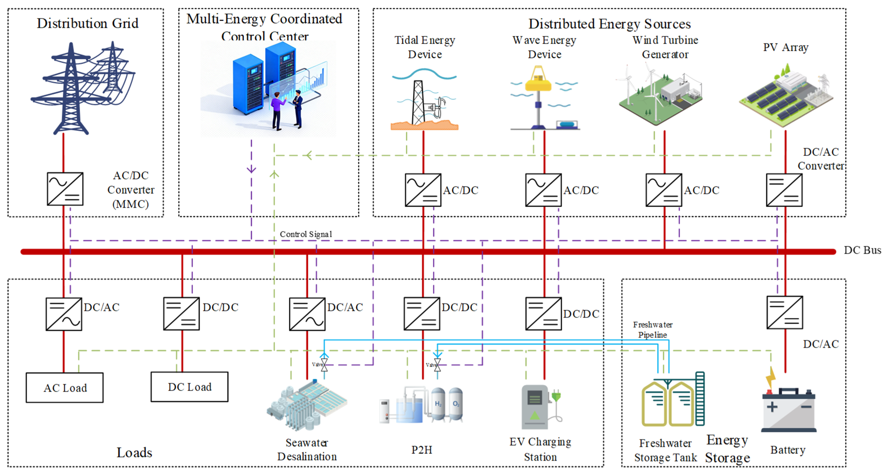
Starting from marine energy, this study establishes a multi-energy coupled direct current (DC) microgrid system. This system integrates renewable energy sources, like PV, wind, tidal current, and wave energy, and flexible loads. The structural layout of the proposed multi-energy coupled DC microgrid system is depicted in Figure 1.
In Figure 1, the DC bus operation is adopted to supply the multi-energy coupling microgrid system, which includes tidal energy devices, wave energy converters, wind turbines, PV arrays, hydrogen production units and EV stations. AC loads are all connected to the DC bus through power electronic converters. A multi-energy complementary control center gathers operational status information of all distributed resources.

3.2. Models of Distributed Energy Generation Units

3.2.1. Wind Power Generation Model

The working principle of wind power generation is that the wind drives the blades of the wind turbine to rotate, generating mechanical energy, which is then converted into electrical energy to supply the power grid. Its model is represented by the following formula.
P W T ( t ) = 0 , v ( t ) < v i n P W T , r v ( t ) v i n v r a t e d v i n , v i n v ( t ) < v r a t e d P W T , r , v r a t e d v ( t ) < v o u t 0 , v ( t ) v o u t
where v ( t ) denotes the wind speed, v i n denotes the cut-in wind speed, v o u t denotes the cut-out wind speed, and v r a t e d denotes the rated wind speed; P W T ( t ) is the output power of the wind turbine, and P W T , r is the rated power of the wind turbine.

3.2.2. Photovoltaic Cell Model

The output power of the photovoltaic cell can be expressed as follows:
P P V ( t ) = η P V ( t ) A P V S t ( t )
where P P V ( t ) denotes the output power, η P V ( t ) denotes the power generation efficiency, A P V represents the total surface area of PV panel, and S t ( t ) denotes the solar irradiance.

3.2.3. Tidal Current Energy Generation Model

The output power fluctuation of tidal current generators is smaller than that of wind turbines. Therefore, this paper does not need to consider the cut-out flow velocity, and its output power can be expressed as follows:
P t i d a l ( t ) = v t i d a l ( t ) v c i t i d a l v r t i d a l v c i t i d a l 3 P r t i d a l , v c i t i d a l v t i d a l ( t ) < v r t i d a l P r t i d a l , v t i d a l ( t ) v r t i d a l 0 , v t i d a l ( t ) < v c i t i d a l
where v t i d a l ( t ) denotes the tidal current velocity, P r t i d a l denotes the rated power, P t i d a l ( t ) denotes the real-time output power, v c i t i d a l denotes the cut-in flow speed, and v r t i d a l denotes the rated flow speed.

3.2.4. Wave Energy Conversion Model

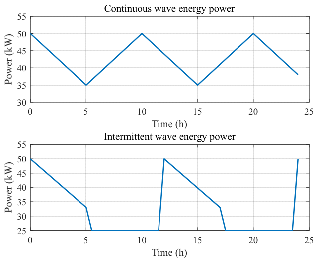
The power output of a Wave Energy Converter (WEC) can be divided into two processes: energy release and energy storage. Under large-wave conditions, the WEC operates continuously, and the accumulator pressure starts to rise before it drops to the valve-closing pressure. At this time, the WEC continues to generate electrical power output even during the energy storage phase. The opposite is also true.
Based on this principle, the time-varying wave energy output power can be expressed using Equations (4) and (5).
P W E G , c ( t ) = P l o w P o p e n T r e l e a s e t + P o p e n , 0 t < T r e l e a s e P l o w P o p e n T a c c ( t T r e l e a s e ) + P l o w , T r e l e a s e t < T W E G
P W E G , i ( t ) = P c l o s e P o p e n T r e l e a s e t + P o p e n , 0 t < T r e l e a s e 0 , T r e l e a s e t < T W E G
where P W E G , c ( t ) and P W E G , i ( t ) denote the wave energy output power at time t under continuous operating conditions and intermittent operating conditions, respectively; P o p e n and P c l o s e denote the electrical output power of the wave energy device corresponding to the accumulator’s valve-opening pressure and valve-closing pressure, respectively; P l o w denotes the minimum output power of the wave energy device under continuous operating conditions; T r e l e a s e denotes the duration of the energy-release process; T a c c denotes the duration of the energy accumulation process; and T W E G denotes the power-output variation period of the wave energy device.
The periodic characteristics of the wave energy power output can be described as:
P WEG , t + T WEG = P WEG ( t )
where P WEG ( t ) denotes the total wave energy output power at time t.

4. Solution Method

4.1. Prediction Model Based on EMD–PCA–LSTM

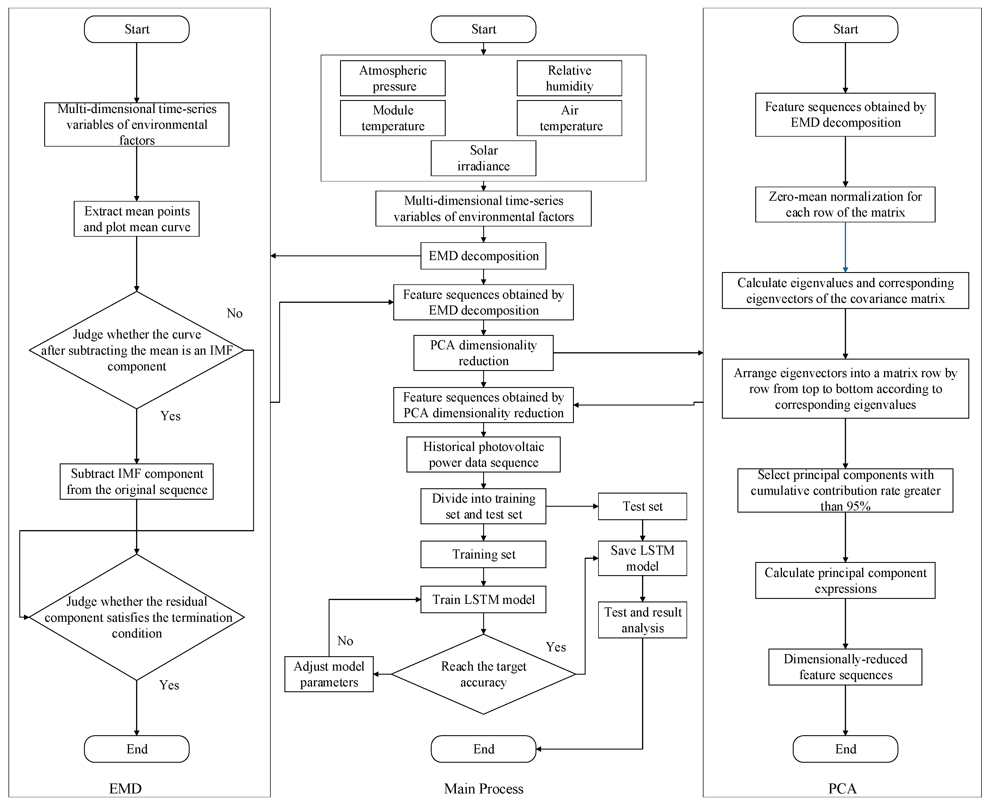
Based on the above discussion, an EMD–PCA–LSTM-based prediction model for renewable energy output power is constructed in this study. In the practical prediction process, a dataset suitable for LSTM model training is first established. The environmental variables and power data at time step t-1 are used to predict the power output at time step t. Figure 2 illustrates the flowchart of the photovoltaic power prediction model based on the EMD–PCA–LSTM neural network.
Input: Renewable energy generation data and environmental variables.
Output: Model evaluation metrics, including RMSE, MAE and R2.
(1)
Data cleaning: The collected photovoltaic power data and environmental data are preprocessed to remove invalid data. Specifically, abnormal or “bad data” caused by communication failures or other operational issues are eliminated on a daily basis.
(2)
EMD decomposition: The environmental data are decomposed into intrinsic mode functions (IMFs) with different frequencies and a residual component r using the EMD algorithm. This process decomposes the original environmental sequences into multiple characteristic fluctuation components, thereby extracting variations and trends at different time scales.
(3)
PCA dimensionality reduction: The decomposed data obtained in Step 2 are further processed using PCA. The PCA algorithm is employed to extract the key factors influencing photovoltaic power output while reducing redundancy and correlation among the multi-scale time series generated by EMD.
(4)
Data normalization: The dimensionally reduced data from Step 3, together with historical photovoltaic power data, are normalized and transformed into a dataset suitable for LSTM training. The dataset is then divided into training and testing sets.
(5)
Model training: The parameters of the LSTM model are initialized, and the training set is input into the model for training until the target accuracy is achieved.
(6)
Model testing: After training is completed, the trained model is saved, and the test set is used for evaluation.
(7)
Evaluation output: The model evaluation indicators RMSE, MAE, and R2 are obtained, and the process ends.
Figure 2 illustrates the overall prediction framework of the proposed EMD–PCA–LSTM model. First, the original environmental and photovoltaic power sequences are preprocessed and decomposed into multiple IMF components through EMD to extract multi-scale fluctuation characteristics. Subsequently, PCA is employed to reduce feature dimensionality and remove redundant information among the decomposed sequences. The processed feature sequences are then input into the LSTM network for model training and prediction. Finally, the prediction performance is evaluated using RMSE, MAE, and R2 indicators. Through the combined effects of decomposition, dimensionality reduction, and deep learning prediction, the proposed framework improves both prediction accuracy and model generalization capability.

4.2. Bi-Level Configuration Model

A bi-level optimization configuration method is adopted to determine the capacity of each resource unit in the system. A bi-level configuration model for joint optimization of flexible resource operation and planning is established so as to effectively coordinate the economic performance and flexibility of systems with a high proportion of renewable energy resources.
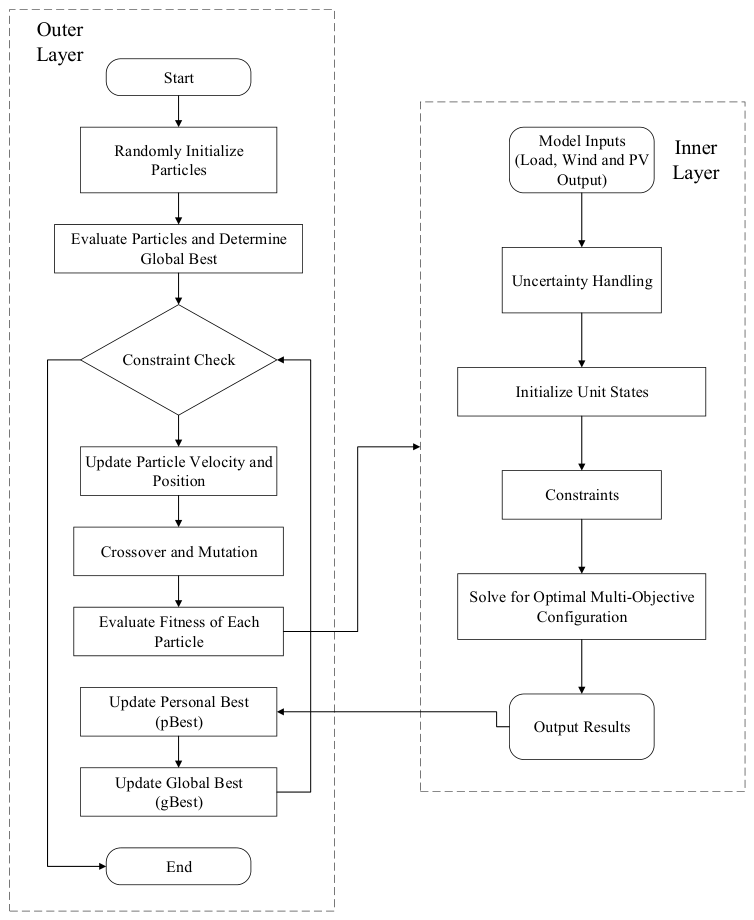
The planning layer and the operation layer interact with each other to jointly determine the optimal configuration scheme of flexible resources. The interaction relationship is shown in Figure 3.
Figure 3 presents the interaction mechanism of the proposed bi-level configuration model. The outer layer mainly focuses on capacity planning and determines the optimal resource allocation scheme through the PSO algorithm. The inner layer is responsible for operational optimization under renewable energy uncertainty and load fluctuations. During the iterative optimization process, the operational results of the inner layer are continuously fed back to the planning layer to update the configuration strategy. Through the interaction between planning and operation, the proposed framework achieves coordinated optimization between economic performance, renewable energy utilization, and system operational reliability.

4.2.1. Operation Layer

(1)
Objective Function
In the operation layer, the performance evaluation metrics such as system operating expenses, system income, and the utilization rate of renewable energy are employed. The aim of this operational stratum is to reduce the total system cost to the lowest possible level by optimizing the output of flexible resources. The formulation of the objective function is presented as follows:
min F 1 = C 1 + c f f e x R
where F 1 denotes the operation-layer objective function; C 1 denotes the system operating cost; R denotes the system revenue; f e x denotes the renewable energy curtailment ratio; and c f is the penalty coefficient used to penalize renewable energy abandonment.
To reduce renewable energy curtailment and improve renewable energy utilization efficiency, a renewable energy abandonment penalty term is introduced as follows:
f e x = i = 1 M P total ( t ) P use ( t ) P total ( t )
The operating cost is presented as follows:
C 1 = c 1 P w t + c 2 P p v + c 3 P t i d e + c 4 P w a v e + c 5 P e s s + c 6 P e v + c 7 P w + c 8 P h 2 + c 9 P g r i d _ b u y
where c1~c9 are coefficients (CNY/kW). P wt and P pv are the output of wind power photovoltaic power (kW). P tide and P wave are the output of tidal current and wave energy (kW), respectively. P ess , P ev , P h 2 and P w are the battery discharge power, electric vehicle power, electrolyzer power, and seawater desalination power (kW), respectively. P grid _ buy and P grid _ sell are the purchased grid power and sold grid power (kW), respectively.
Equation (9) expresses the total operating cost of the offshore integrated energy system as the sum of the operating costs of different energy generation, storage, and flexible load units. Therefore, nine cost coefficients are introduced to characterize the operating costs of wind power, photovoltaic power, tidal energy, wave energy, battery storage, electric vehicles, seawater desalination, hydrogen production, and grid electricity purchase, respectively.
The revenue is presented as follows:
R = r 1 P e v + r 2 P w + r 3 P h 2 + r 4 P g r i d _ s e l l
where r1~r4 are the revenue coefficients (CNY/kW).
Equation (10) represents the total system revenue. Four revenue coefficients are introduced because only electric vehicle services, seawater desalination, hydrogen production, and electricity sales to the external grid can directly generate economic benefits in the proposed offshore integrated energy system.
The operational constraints mainly include power balance constraints, ramping constraints, hydrogen production constraints, and energy storage SOC constraints to ensure stable system operation.
(2)
Operational Constraints
Power constraints of each unit are presented as follows:
P w t , min < P w t < P w t , max P p v , min < P p v < P p v , max P t i d e , min < P t i d e < P t i d e , max P w a v e , min < P w a v e < P w a v e , max P e v , min < P e v < P e v , max P w , min < P w < P w , max P h 2 , min < P h 2 < P h 2 , max
Ramping constraints are presented as follows:
0 < d P w < d P w , max
The constraints of hydrogen production and freshwater output are presented as follows:
Q P w , min < Q P w < Q P w , max
Q P h 2 , min < Q P h 2 < Q P h 2 , max
The state of charge (SOC) is updated and presented as follows:
E ba ( t + 1 ) = E ba ( t ) + P t b a , c η ba , c P t b a , d η ba , d Δ t , t T .
0 P t b a , c P max b a , c
0 P t b a , d P max b a , d
The SOC remain within the safe operating range, which is presented as follows:
S OC ( t ) = E ba ( t ) / E ba , 0
S OC , min S OC ( t ) S OC , max
The energy storage system cannot charge and discharge simultaneously, which is presented as follows:
P t b a , d P t b a , c = 0

4.2.2. Planning Layer

(1)
Objective Function
In the planning layer, system investment indicators are incorporated into the evaluation framework. The objective of the planning layer is to minimize the annual total cost of the system, and the objective function is presented as follows:
min F 2 = F 1 + C 2
where F 2 is the objective function, and C 2 is the investment cost.
The annualized investment cost of the system is presented as follows:
C 2 = r ( 1 + r ) n ( 1 + r ) n 1 i = 1 N 0 c i P i
where r denotes the discount rate, n denotes the project lifetime, c i denotes the unit investment cost of the i-th energy component, P i denotes the installed capacity of the corresponding component, and N 0 denotes the total number of energy components considered in the planning model.
(2)
Constraints
The constraints on the number of units are presented as follows:
N W T , min < N W T < N W T , max N P V , min < N P V < N P V , max N W A V E , min < N W A V E < N W A V E , max N T I , min < N T I < N T I , max N E S S , min < N E S S < N E S S , max
where N W T , min , N P V , min , N W A V E , min , N T I , min , and N E S S , min denote the minimum allowable numbers of wind turbine units, photovoltaic units, wave energy units, tidal current energy units, and battery storage units, respectively; N W T , max , N P V , max , N W A V E , max , N T I , max and N E S S , max denote the corresponding maximum allowable numbers.

5. CVaR-Based Risk Planning Model

In the capacity configuration optimization problem, if only the expected cost is taken as a single optimization objective, various uncertainty factors tend to be averaged, making it difficult to fully reflect the impacts of tail-risk scenarios such as fluctuations in renewable energy output, sudden load increases, and extreme electricity price variations on system economy and operational security. This may lead to situations where the configured scheme suffers from significant cost overruns or power supply–demand imbalance under extreme operating conditions. To achieve an interpretable, quantifiable, and optimizable balance between system economy and operational robustness, Conditional Value at Risk (CVaR) is introduced in this chapter as a tail risk measurement indicator [27].
CVaR is a risk measure developed on the basis of Value at Risk (VaR). Unlike VaR, which only reflects the quantile loss at a given confidence level, CVaR further characterizes the mean value of all extreme losses below that quantile, effectively compensating for the limitation of VaR in describing tail risks. As a coherent risk measure, CVaR satisfies mathematical properties such as subadditivity, monotonicity, positive homogeneity, and translation invariance. While ensuring the model remains solvable and easy to optimize, it enables a more accurate assessment of potential system risks [28]. Its mathematical expression is given as follows:
δ = α + 1 1 β y R [ f ( x , y ) α ] + ρ ( y ) d y
where δ denotes the CVaR value; α denotes the VaR value at confidence level β ; f ( x , y ) denotes the loss function; x denotes the decision variables of the planning model, such as installed capacities of different energy units; y denotes the stochastic variables associated with renewable energy output uncertainty and load fluctuations; ρ ( y ) denotes the probability density function of y; and [ f ( x , y ) α ] + denotes max [ 0 , f ( x , y ) α ] + .
In general, the probability density function is difficult to obtain, and the integral term contained in Equation (24) makes the computation relatively complex. Therefore, for convenience in solving, Equation (24) can be estimated and discretized by using the historical data of the random variables. The expression is given as follows:
δ ˜ = α + 1 m ( 1 β ) i = 1 m [ f ( x , y i ) α ] +
where δ ˜ denotes the estimated value of CVaR, m denotes the total number of samples, and y i denotes the i-th sample.
After considering uncertainty risks, a weighted sum method is adopted to balance the profit and risk of the virtual power plant (VPP). The final day-ahead optimal scheduling model of the VPP is formulated as follows:
max { ( 1 ζ ) s = 1 N ρ s F s , 1 ζ ( φ + 1 N ( 1 β ) s = 1 N ρ s η s ) }
f vpp DA , s φ η s 0 , η s 0
where ζ denotes the risk preference coefficient, whose value lies in the range of 0 to 1, representing the degree of risk preference of the VPP; a larger ζ indicates that the VPP is more conservative; and a smaller ζ indicates a higher preference for risk. N denotes the set of scenarios, ρ s denotes the probability of scenario s, φ denotes the VaR value of the VPP profit, β denotes the confidence level, and η s is an auxiliary variable representing the amount by which the VPP profit in scenario s exceeds φ .

6. Case Study Analysis

6.1. Basic Data

The basic parameters of the offshore integrated energy system are presented in Table 1, Table 2 and Table 3, including the rated capacity, investment cost, service lifetime, and equivalent levelized cost parameters of different units. The parameter settings are determined based on engineering practice and relevant literature to ensure the operational feasibility and economic rationality of the proposed system.
Table 1 presents the rated capacities of renewable generation units, storage systems, and flexible loads. Table 2 provides the investment cost and lifetime parameters used for calculating the annualized investment cost in the planning layer. Table 3 summarizes the equivalent economic coefficients of different units. For renewable generation units, including wind power, solar power, wave energy, and tidal energy, the coefficients correspond to conventional levelized cost of electricity (LCOE) values. For flexible demand-side units such as EV charging, hydrogen production, and seawater desalination, the equivalent coefficients are calculated by considering both operational expenditure and service revenues.
The equivalent levelized economic cost coefficient is calculated as follows:
L C O E = C i n v + C o p e + C m a i n B E t o t a l
where C i n v denotes the investment cost, C o p e denotes the operational cost, C m a i n denotes the maintenance cost, B denotes the economic benefit or operational revenue, and E t o t a l represents the total equivalent energy output during the lifecycle.
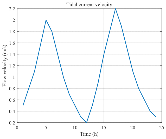
The tidal current velocity profile and periodic output characteristics of wave energy generation are presented in Figure 4 and Figure 5. As shown in Figure 4, the tidal current velocity exhibits obvious periodic fluctuation characteristics within a 24 h cycle, with two significant peak periods occurring around 5 h and 17 h. The maximum tidal current velocity reaches approximately 2.2 m/s, while the minimum value decreases to approximately 0.2 m/s, indicating strong temporal variability of tidal energy resources.
Figure 5 illustrates the output characteristics of the wave energy generation device under continuous and intermittent operating conditions. Under continuous operating conditions, the output power fluctuates within a relatively stable range and maintains continuous power supply capability. In contrast, under intermittent operating conditions, the output power periodically decreases to zero during part of the operating cycle, resulting in discontinuous output characteristics. For this study, the wave energy device is assumed to operate under large-wave conditions throughout the scheduling period; therefore, the continuous operating mode is adopted in the subsequent analysis.

6.2. Analysis of Prediction Results

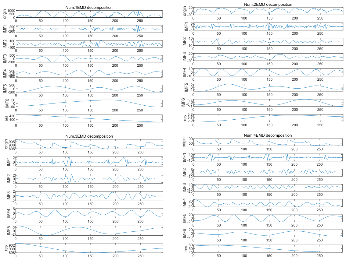
The environmental sequence data in the experimental samples are non-stationary signals. Due to the influence of weather variations, they exhibit certain randomness and abrupt changes. In this study, the EMD algorithm is adopted to decompose the original environmental sequence data into intrinsic mode function (IMF) components and residual components for each environmental factor, so as to highlight the local characteristics of the original environmental sequences. The photovoltaic forecasting dataset used in this study consists of solar irradiance, air temperature, air pressure, humidity, and photovoltaic output power data. After preprocessing and abnormal data cleaning, a total of 6952 time-series samples are obtained for model training and testing.
The decomposition results are shown in the following figure.
Figure 6 shows the EMD decomposition results of the photovoltaic-related meteorological feature sequences, including solar irradiance, air temperature, air pressure, and humidity. Each original feature sequence is decomposed into several intrinsic mode function (IMF) components and one residual component to extract multi-scale fluctuation characteristics. The high-frequency IMF components mainly represent short-term environmental disturbances and random fluctuations, whereas the low-frequency components and residual terms reflect long-term variation trends and periodic characteristics. Compared with the original non-stationary sequences, the decomposed subsequences exhibit clearer temporal patterns and reduced complexity, which is beneficial for improving the prediction capability of the subsequent LSTM model.
The four subfigures in Figure 6 correspond to the EMD decomposition results of solar irradiance, air temperature, air pressure, and humidity feature sequences, respectively. The number of IMF components is determined adaptively by the EMD algorithm according to the characteristics of each feature sequence, rather than being manually predefined. Furthermore, PCA is employed to retain the principal components with cumulative contribution rates exceeding 90%, thereby reducing data redundancy and improving prediction efficiency.
To ensure fair comparison, the three prediction models adopt the same LSTM network architecture and training hyperparameters, while only the input feature processing methods are different. The main hyperparameter settings of the prediction models are summarized in Table 4.
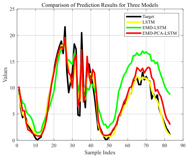
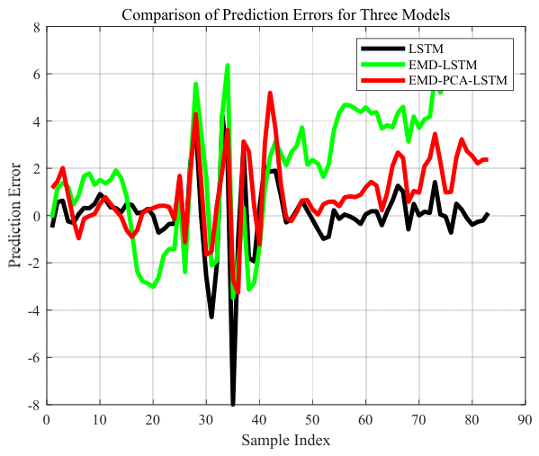
From the Figure 7, Figure 8 and Table 5, it can be seen that in the test dataset, as the number of input variables increases, the RMSE and MAE of the EMD–LSTM model increase, while the R2 decreases, indicating a certain decline in the prediction accuracy of the model, which is consistent with the expectation before the experiment.
However, when principal component analysis is applied to reduce the original input variables to 9 variables, the RMSE and MAE of the EMD–PCA–LSTM prediction model are reduced by 32% and 25%, respectively, compared with the single LSTM model, demonstrating the necessity of PCA dimensionality reduction.
Moreover, the prediction accuracy and performance of the EMD–PCA–LSTM model are higher than those of the other comparison models. The results also indicate that directly introducing EMD-decomposed high-dimensional feature sequences into the LSTM network may increase data redundancy and model complexity, thereby reducing prediction accuracy. After PCA dimensionality reduction, redundant and highly correlated feature information is effectively removed, enabling the LSTM network to better extract representative temporal characteristics from the decomposed sequences. Therefore, the EMD–PCA–LSTM model achieves better prediction stability and generalization capability than the traditional LSTM and EMD–LSTM models.

6.3. Analysis of Capacity Configuration Optimization Results

Table 1 provides the rated capacity of each individual unit, whereas Table 6 presents the optimized installed capacities obtained from the configuration optimization model. Considering the nonlinear and multi-constraint characteristics of the offshore integrated energy system planning problem, the particle swarm optimization (PSO) algorithm is adopted due to its strong global search capability and fast convergence performance. Through the PSO algorithm, the capacity configuration results are obtained. Different risk preference coefficients will affect the CVaR risk value and the final configuration results of energy storage. Therefore, ζ is set to 0.05, 0.1, 0.2, 0.4, 0.6, 0.8, and 1 (with β = 0.9), and different CVaR risk values and resource configurations are obtained.
In this study, the selected configuration scheme includes a wind power unit of 4500 kW, a photovoltaic unit of 2100 kW, a tidal current unit of 1050 kW, a wave energy unit of 1000 kW, and an energy storage capacity of 2400 kW. Under this configuration, the net cost is minimized to 1.19 × 10⁷, and the curtailment rate is only 0.7%.
It can be seen from Table 6 that as the risk preference coefficient increases, the equivalent annual total construction and operation cost of the VPP increases, while the risk cost gradually decreases. This indicates that the investor becomes more risk-averse, and the planning strategy tends to be more conservative.
Table 6 intuitively reveals the impact of the risk aversion coefficient on the optimal configuration strategy of the virtual power plant (VPP). When the risk aversion coefficient ( ζ ) is at a low level, the objective function of the optimization model is mainly dominated by the expected cost. In this case, the capacity configuration scheme exhibits risk neutrality and aims to minimize the average operating cost across all scenarios. As a result, the initial investment of the configuration may be relatively low, but at the expense of a higher conditional value at risk (CVaR).
As the risk preference coefficient gradually increases, the VPP mainly focuses on satisfying load demand and reducing the risks caused by uncertainty fluctuations. Energy storage can meet load demand when there is a generation deficit and can flexibly charge and discharge according to electricity prices to adjust the amount of power purchased and sold. When the risk coefficient increases, the proportion of energy storage configuration increases accordingly, while curtailment and power trading volumes decrease, leading to a reduction in risk.
Based on the above analysis, it can be concluded that in capacity configuration, the balance between profit and risk can be achieved by adjusting the risk preference coefficient, thereby enabling a reasonable selection of the configuration strategy.

6.4. Analysis of System Optimal Scheduling Results

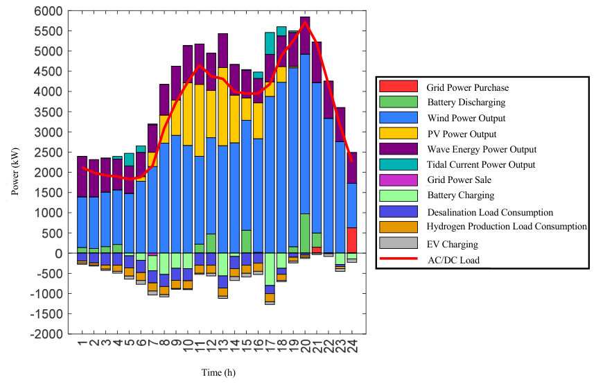
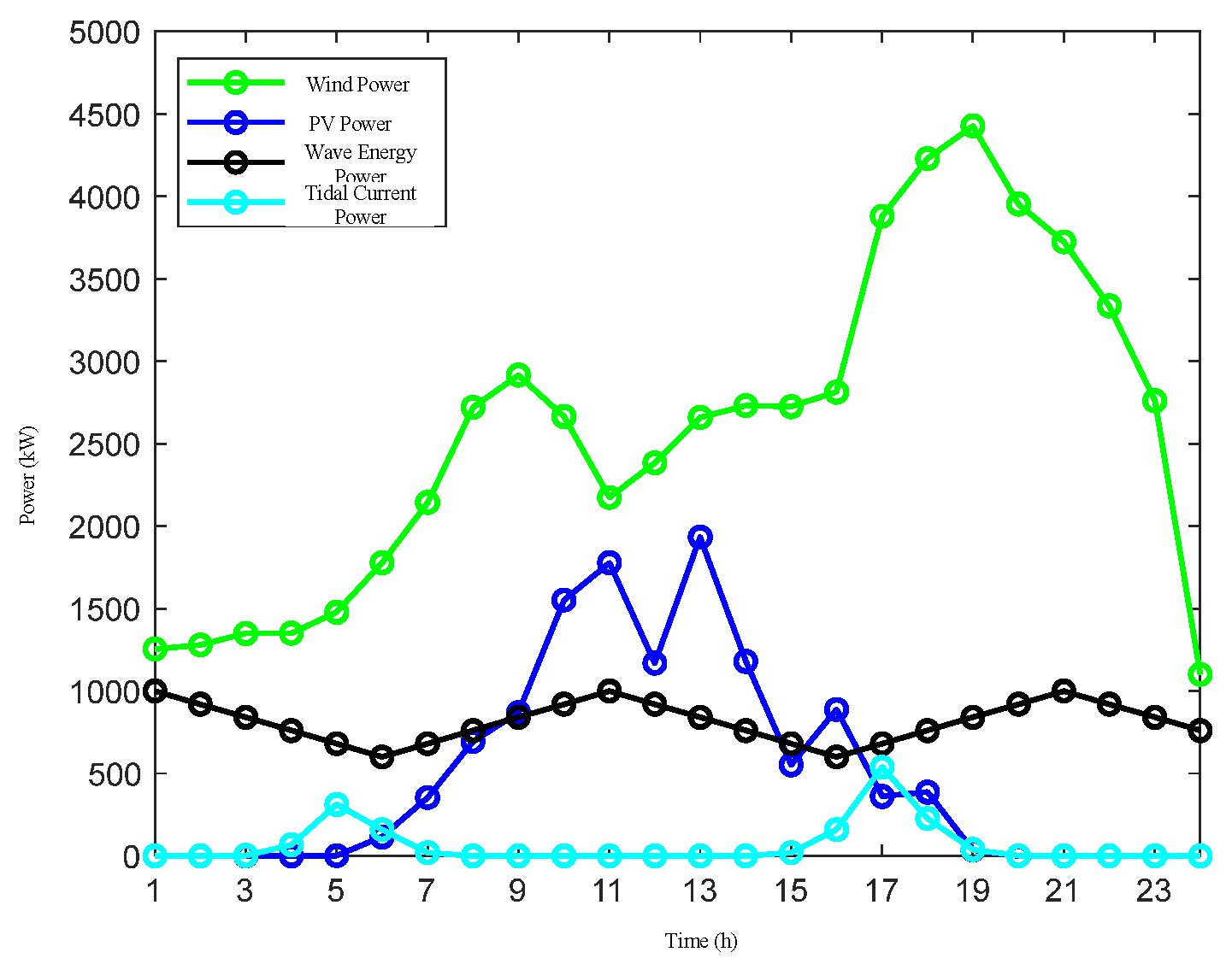
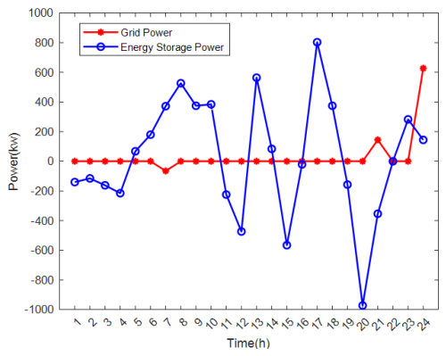
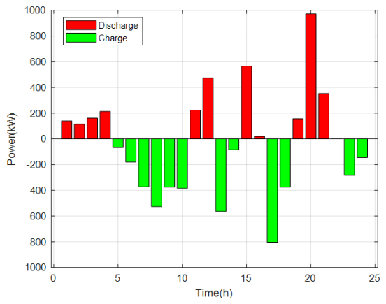
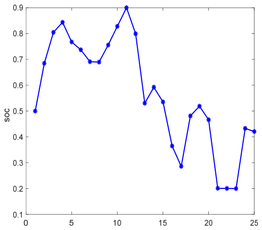
The results of day-ahead scheduling are presented in Figure 9, Figure 10, Figure 11, Figure 12 and Figure 13. Under the optimal capacity configuration, renewable energy generation is plentiful. Figure 10 illustrates the output of various renewable energy sources, with wind power being the most abundant among them. Photovoltaic power generation operates from 7:00 to 18:00. Tidal energy, shaped by the gravitational interactions among the Earth, the Moon, and the Sun, gives rise to two high tides and two low tides each day, with a cycle lasting approximately 12 h and 24 min (semi-diurnal tide). This results in a periodic fluctuation in tidal current output throughout the day. Wave energy generation varies between 600 and 420 under high-wave conditions. The system adheres to power balance constraints, and renewable energy generation is ample. The desalination unit, electric vehicles, and hydrogen production units fully utilize the surplus renewable energy, enabling multi-channel profit generation. The energy storage output is depicted in Figure 12 and Figure 13. During periods of low electricity prices, the storage system charges to accumulate energy, while during periods of high electricity prices, it discharges to generate electricity, thereby further enhancing revenue. Simultaneously, it is ensured that the difference between the state of charge at the end of the day and the initial state of charge remains within 5%.

7. Conclusions

This paper takes an offshore multi-energy coupled system as the research object and conducts a systematic study on capacity optimization and risk-based scheduling under uncertain environments. A two-stage optimization framework that considers both economic efficiency and reliability is proposed. The main conclusions are as follows:
(1)
A multi-energy coupled system model including wind energy, photovoltaic, tidal current energy, wave energy, energy storage, hydrogen production via electrolysis, and desalination load is constructed. The complementary relationships among different energy units and the energy flow paths are systematically characterized, laying a foundation for the optimal operation of offshore integrated energy systems.
(2)
To address the high uncertainty of renewable energy and load, a hybrid prediction model based on EMD–PCA–LSTM is developed. Through decomposition, denoising, and feature extraction of the original sequences, the model significantly improves prediction accuracy and provides reliable data input for subsequent optimal scheduling.
(3)
A bi-level capacity configuration method based on joint operation–planning optimization is proposed. At the planning layer, Conditional Value at Risk (CVaR) is innovatively introduced to quantify the economic risk under extreme scenarios. With the minimization of the annualized total system cost and risk cost as the combined objective, an optimal balance between economic performance and robustness of energy and storage units is achieved.
(4)
The results verify the feasibility and superiority of the proposed method. The proposed framework effectively improves renewable energy accommodation and reduces the renewable energy curtailment rate to 0.7%. Meanwhile, the EMD–PCA–LSTM prediction model achieves higher prediction accuracy and better generalization capability compared with traditional LSTM-based models. Through the coordinated effects of high-accuracy prediction, risk-quantified decision-making, and bi-level scheduling optimization, the proposed method enhances both economic performance and operational stability of offshore integrated energy systems.
Future work can further deepen uncertainty modeling, explore data-driven stochastic optimization and distributionally robust optimization methods, and incorporate market response mechanisms and multi-agent game theory to investigate coordinated decision-making of energy storage control strategies and multi-party interests, thereby promoting the intelligent and market-oriented development of offshore integrated energy systems.

Author Contributions

Conceptualization, H.F.; methodology, H.F. and Y.L.; validation, H.F., Y.L. and Z.C.; investigation, Y.L., Z.C., C.W. and W.W.; resources, Y.L., and C.W.; software, Z.C.; data curation, Z.C., C.W. and W.W.; writing—original draft, Y.L. and H.F.; writing—review and editing, H.F.; formal analysis, C.W. and W.W.; visualization, W.W., supervision, H.F. All authors have read and agreed to the published version of the manuscript.

Funding

This research received no external funding.

Data Availability Statement

The original contributions presented in this study are included in the article. Further inquiries can be directed to the corresponding author.

Conflicts of Interest

Author Yan Liu, Cui Wang, and Wankun Wang were employed by the company China Datang Technology Innovation Co., Ltd. The remaining authors declare that the research was conducted in the absence of any commercial or financial relationships that could be construed as a potential conflict of interest.

Nomenclature

Abbreviations
AbbreviationDescription
ACAlternating current
DCDirect current
IESIntegrated energy system
VPPVirtual power plant
PVPhotovoltaic
WTWind turbine
WECWave energy converter
ESSEnergy storage system
EVElectric vehicle
EMDEmpirical mode decomposition
PCAPrincipal component analysis
IMFIntrinsic mode function
LSTMLong short-term memory
RNNRecurrent neural network
PSOParticle swarm optimization
CVaRConditional value-at-risk
VaRValue-at-risk
SOCState of charge
RMSERoot mean square error
MAEMean absolute error
R2Coefficient of determination
LCOELevelized cost of electricity
Indices
SymbolDescription
t Index of time period
s Index of scenario
i Index of energy component
N Set of scenarios
m Total number of samples
N 0 Total number of energy components considered in the planning model
Variables and Parameters
SymbolDescription
P W T ( t ) Output power of the wind turbine at time t
P P V ( t ) Output power of photovoltaic generation at time t
P t i d a l ( t ) Real-time output power of tidal current generation at time t
P W E G , c ( t ) Wave energy output power under continuous operating conditions at time t
P W E G , i ( t ) Wave energy output power under intermittent operating conditions at time t
P WEG ( t ) Total wave energy output power at time t
F 1 Objective function of the operation layer
F 2 Objective function of the planning layer
C 1 System operating cost
C 2 Investment cost
R System revenue
f e x Renewable energy curtailment ratio
c f Penalty coefficient for renewable energy curtailment
P total ( t ) Total available renewable energy power at time t
P use ( t ) Utilized renewable energy power at time t
c 1 ~ c 9 Operating cost coefficients of different system units
r 1 ~ r 4 Revenue coefficients of flexible loads and electricity sales
P wt Wind power output
P pv Photovoltaic power output
P tide Tidal current power output
P wave Wave energy power output
P ess Battery discharge power
P ev Electric vehicle power
P w Seawater desalination power
P h 2 Electrolyzer power
P grid _ buy Purchased power from the external grid
P grid _ sell Sold power to the external grid
E ba ( t ) Stored energy of the battery at time t
P t b a , c Battery charging power at time t
P t b a , d Battery discharging power at time t
η ba , c Battery charging efficiency
η ba , d Battery discharging efficiency
Δ t Time interval
S OC ( t ) State of charge of the energy storage system at time t
r Discount rate
n Project lifetime
c i Unit investment cost of the i -th energy component
P i Installed capacity of the i -th energy component
N W T Number of wind turbine units
N P V Number of photovoltaic units
N W A V E Number of wave energy units
N T I Number of tidal current energy units
N E S S Number of energy storage units
δ CVaR value
δ ˜ Estimated value of CVaR
α VaR value at confidence level β
β Confidence level
f ( x , y ) Loss function
x Decision variables of the planning model
y Stochastic variables associated with renewable energy output and load fluctuations
ρ ( y ) Probability density function of y
y i The i -th sample of the stochastic variable
ζ Risk preference coefficient
ρ s Probability of scenario s
F s , 1 Profit or objective value under scenario s
φ VaR value of VPP profit
η s Auxiliary variable representing the excess of VPP profit over φ in scenario s
f vpp DA , s Day-ahead profit of the VPP under scenario s
C i n v Investment cost in LCOE calculation
C o p e Operational cost in LCOE calculation
C m a i n Maintenance cost in LCOE calculation
B Economic benefit or operational revenue
E t o t a l Total equivalent energy output during the lifecycle

Appendix A. Mathematical Formulations of the RNN and LSTM Networks

For a given sequence x = (x1, x2, …,xn), the iterative computation of the RNN structure is expressed as shown in Equations (A1) and (A2).
h t = f a W x h x t + W h h h t 1 + b h
y t = W h y h t + b y  
where W denotes the weight matrix, b denotes the bias vector, f a represents the activation function, and the subscript t denotes the time step.
By introducing gating mechanisms, the LSTM effectively addresses the issues of gradient vanishing and explosion in traditional RNNs, making deep neural networks unfolded over time easier to train. The forward computation process of the LSTM is described in Equations (A3)–(A7).
i t = σ W x i x t + W h i h t 1 + W c i c t 1 + b i  
f t = σ W x f x t + W h f h t 1 + W c f c t 1 + b f  
c t = f t c t 1 + i t tanh W x c x t + W h c h t 1 + b c  
o t = σ W x o x t + W h o h t 1 + W c o c t + b o
h t = o t tanh ( c t )  
where i denotes the input gate, f denotes the forget gate, c denotes the cell state, and o denotes the output gate; W represents the corresponding weight matrices, b represents the corresponding bias terms, σ denotes the sigmoid activation function, and tanh denotes the hyperbolic tangent activation function.

References

  1. Xiong, B.; Wang, D.; Hao, S.; Wang, Z.; Zhang, C.; Huang, M.; Li, S.; Xiao, G. Opportunities, challenges, and perspectives on the high-quality development of new energy driven by global energy transition. Acta Pet. Sin. 2026, 47, 74–94. [Google Scholar]
  2. Chen, L.; Liao, Y.; Pan, Q.; Wu, C.; Wang, Z. Integration of Wind-Solar-Wave-Current Energy and Water Transportation: Current Status and Prospects. J. Chang. Univ. Sci. Technol. (Nat. Sci.) 2026, 23, 68–86. [Google Scholar]
  3. Wu, F.; Ju, P.; Qin, C.; Li, L.; Tao, A.; Sun, L. Progress and prospect of research on offshore renewable energy generation. J. Hohai Univ. (Nat. Sci.) 2014, 42, 80–87. [Google Scholar]
  4. Du, W.J.; Cai, G.T.; Qi, X.L.; Wang, P.; Zhang, J.X. Review on development and utilization of offshore renewable energy: An analysis based on a five-dimensional framework. Resour. Sci. 2025, 47, 675–690. [Google Scholar]
  5. Liu, S.G.; Zhang, P.; Zhao, X.Y. Study on integrated development and utilization modes of China’s offshore renewable energy from the perspective of new-quality productivity. Resour. Sci. 2025, 47, 691–702. [Google Scholar]
  6. Michaelis, D. Energy Island. In OCEANS 2003. Celebrating the Past … Teaming Toward the Future; IEEE: San Diego, CA, USA, 2003; Volume 4, pp. 2294–2302. [Google Scholar] [CrossRef]
  7. Liu, S. Design and Research on Foundational Platform of Offshore Complementary Power System with Wind and Wave Energy. Master’s Thesis, North China Electric Power University, Beijing, China, 2014. (In Chinese) [Google Scholar]
  8. Lü, C.; Liu, S.; Wang, S.; Lan, Y.; Rao, Y. Discussion on advances in power generation equipment and technology for marine renewable energy and its issues. J. Hydroelectr. Eng. 2015, 34, 195–198. [Google Scholar]
  9. Wang, S.; Li, Z.; Yu, T.; Ma, C. A review of research on multi-energy complementary ocean energy integrated power generation technology. Mar. Sci. Bull. 2019, 38, 241–249. [Google Scholar]
  10. Yu, H. Design and Application of the Wind-Photovotaic-Storage Complementary Microgrid System. Sci. Technol. Inf. 2023, 21, 94–97. [Google Scholar]
  11. Delbeke, O.; Bastianel, G.; Yurtseven, K.; Ergun, H.; Moschner, J.D.; Driesen, J. Hybrid offshore solar-wind farms: The potential of integrating floating photovoltaics with offshore wind. Appl. Energy 2026, 410, 127486. [Google Scholar] [CrossRef]
  12. Shi, X.; Chen, J.; Gao, Q.; Tang, P.; He, F. Complementary value of wave and tidal current energy in the power grid and their impact on balanced energy demand. Renew. Energy 2026, 261, 125311. [Google Scholar] [CrossRef]
  13. Li, P.; Lian, J.; Ma, C.; Zhang, J. Complementarity and development potential assessment of offshore wind and solar resources in China seas. Energy Convers. Manag. 2023, 296, 117705. [Google Scholar] [CrossRef]
  14. An, L.; Wang, M.; Qi, X.; Li, F.; Qu, T. Optimal dispatching of multi-power sources containing wind/photovoltaic/thermal/hydro-pumped and battery storage. Renew. Energy 2018, 36, 1492–1498. [Google Scholar]
  15. Ma, X.; Liang, C.; Dong, X.; Li, Y. Multi-objective reactive power optimization strategy of power system considering large-scale renewable integration. Front. Energy Res. 2023, 11, 1213154. [Google Scholar] [CrossRef]
  16. Li, X.; Wang, X.; Gu, J.; Xu, J. Day-Ahead Optimal Dispatching of Wind-Solar-Thermal Power Storage System Considering Deep Peak Shaving of Thermal Power. China Electr. Power 2023, 56, 1–7+48. [Google Scholar]
  17. Nan, B.; Jiang, C.; Dong, S.; Xu, C. Day-ahead and Intra-day Coordinated Optimal Scheduling of Integrated Energy System Considering Uncertainties in Source and Load. Power Syst. Technol. 2023, 47, 3669–3683. [Google Scholar]
  18. Zhu, Y.; Geng, Q. Capacity Allocation and Operation Optimization of Integrated Energy Park System Coupled with Hydrogen Energy Storage. Mod. Electr. Power 2023, 40, 931–938. [Google Scholar]
  19. Li, R.; Zhang, X.; Xu, Y.; Sun, W.; Zhou, X.; Guo, C.; Chen, H. Research on optimal configuration of hybrid energy storage capacity for wind-solar generation system. Energy Storage Sci. Technol. 2019, 8, 512–522. [Google Scholar]
  20. Zhang, Y.; Sun, H.; Tan, J.; Li, Z.; Hou, W.; Guo, Y. Capacity configuration optimization of multi-energy system integrating wind turbine/photovoltaic/hydrogen/battery. Energy 2022, 252, 124046. [Google Scholar] [CrossRef]
  21. Fu, J.; Zeng, G.; Ji, Y.; Zhou, A. Development of a Capacity Allocation Model for the Multi-Energy Hybrid Power System. J. Therm. Sci. 2025, 34, 936–952. [Google Scholar] [CrossRef]
  22. Yang, T.; Yang, Z.; Li, F.; Wang, H. A short-term wind power forecasting method based on multivariate signal decomposition and variable selection. Appl. Energy 2024, 360, 122759. [Google Scholar] [CrossRef]
  23. Sharief Basha, S.; Nagaraja Rao, A.; Nida Fariz, T.K. Dimensionality reduction in solar radiation forecasting: A combined PCA-SVM framework for renewable energy applications. Front. Environ. Sci. 2025, 13, 1692076. [Google Scholar] [CrossRef]
  24. Kanagarathinam, K.; Aruna, S.K.; Ravivarman, S.; Safran, M.; Alfarhood, S.; Alrajhi, W. Enhancing sustainable urban energy management through short-term wind power forecasting using LSTM neural network. Sustainability 2023, 15, 13424. [Google Scholar] [CrossRef]
  25. Guo, Y.; Ming, B.; Huang, Q.; Wang, Y.; Li, Y. Day-Ahead Robust Optimal Scheduling of Hydro-Wind-PV-Storage Complementary System Considering the Steadiness of Power Delivery. Trans. China Electrotech. Soc. 2023, 38, 2350–2363. [Google Scholar]
  26. Zhang, J.; Zhu, Y.; Li, X.; Liu, L. Optimization Scheduling Strategy of Offshore Wind Farm Power System Considering Wind Power Uncertainty. Distrib. Energy 2021, 6, 33–43. [Google Scholar]
  27. Rockafellar, R.T.; Uryasev, S. Optimization of Conditional Value-at-Risk. J. Risk 2000, 2, 21–42. [Google Scholar] [CrossRef]
  28. Inzunza, A.; Moreno, R.; Bernales, A.; Rudnick, H. CVaR-constrained planning of renewable generation with consideration of system inertial response, reserve services and demand participation. Energy Econ. 2016, 59, 104–117. [Google Scholar] [CrossRef]
  29. Fan, H.; Liu, Y.; Wang, C.; Wang, W. Capacity Optimization and Rolling Scheduling of Offshore Multi-Energy Coupling Systems. Energies 2026, 19, 447. [Google Scholar] [CrossRef]
Figure 1. Structure of the Multi-Energy Coupling DC Microgrid System.
Energies 19 02585 g001
Figure 2. Flowchart of photovoltaic output power prediction based on EMD–PCA–LSTM.
Energies 19 02585 g002
Figure 3. Flowchart of Capacity Configuration.
Energies 19 02585 g003
Figure 4. Tidal Current Velocity.
Energies 19 02585 g004
Figure 5. Periodic output of wave energy generation power.
Energies 19 02585 g005
Figure 6. EMD decomposition results.
Energies 19 02585 g006
Figure 7. Photovoltaic power prediction results.
Energies 19 02585 g007
Figure 8. Comparison of prediction errors.
Energies 19 02585 g008
Figure 9. Day-ahead total resource output [29].
Energies 19 02585 g009
Figure 10. Renewable energy generation output [29].
Energies 19 02585 g010
Figure 11. Power exchange profile [29].
Energies 19 02585 g011
Figure 12. Energy storage output [29].
Energies 19 02585 g012
Figure 13. State of charge (SOC) [29].
Energies 19 02585 g013
Table 1. Rated Capacity.
Unit TypeWind PowerEVSolar PowerSeawater DesalinationWave EnergyHydrogen ProductionTidal EnergyBattery
Capacity per Unit (kW)150020065005020070300
Table 2. Investment Cost.
Unit TypeWind PowerSolar Power Wave Energy Tidal EnergyBattery
Investment Cost (CNY/kW)14,000580020,00016,0001500
Lifetime (years)3020252510
Table 3. Equivalent Levelized Economic Cost Parameters.
Unit TypeWind PowerSolar PowerWave EnergyTidalBatteryEVHydrogen ProductionSeawater Desalination
LCOE (CNY/kW)0.150.10.30.250.13−0.5−0.7−0.8
Table 4. Hyperparameter settings of the prediction models.
Time StepInput DimensionHidden LayersHidden UnitsOutput DimensionBatch SizeTraining EpochsTraining SamplesTest Samples
1915011050048662086
Table 5. Comparison of prediction results.
ModelRMSEMAER2
LSTM1.8511.0320.886
EMD-LSTM3.6763.1920.551
EMD-PCA-LSTM1.2590.7770.929
RMSE and MAE are used to evaluate prediction errors, while R2 reflects the fitting performance and generalization capability of the prediction model.
Table 6. Configuration results under different risk preference coefficients.
Risk CoefficientWind UnitsPV UnitsESS UnitsTidal UnitsWave UnitsNet Cost
(107 yuan)
CVaR Cost
(107 yuan)
0.053350815201.1901.349
0.143261013221.1961.337
0.242471314211.2111.322
0.443331314211.2371.318
0.643881714211.2661.315
0.852182113211.2831.304
152002914201.3051.295
Disclaimer/Publisher’s Note: The statements, opinions and data contained in all publications are solely those of the individual author(s) and contributor(s) and not of MDPI and/or the editor(s). MDPI and/or the editor(s) disclaim responsibility for any injury to people or property resulting from any ideas, methods, instructions or products referred to in the content.