Coordinated Planning of Flexible Interconnection and Grid-Forming Energy Storage in Low-Voltage Distribution Networks Considering Off-Grid Operation

Abstract

Severe weather events increasingly threaten the reliability of low-voltage distribution networks (LVDNs). Existing fault restoration strategies primarily focus on medium-voltage networks, leaving LVDNs highly vulnerable during prolonged grid outages. To enhance the off-grid operation capability of LVDNs, this paper proposes a coordinated planning model integrating flexible interconnection devices and grid-forming energy storage systems (GFM-ESSs). First, this study develops a hierarchical planning framework for LVDNs to jointly optimize the allocation of soft open points (SOPs) and grid-forming energy storage systems (GFM-ESSs), with the aim of reducing both interruption-related losses and equipment investment in distribution transformer areas. Second, active support capability evaluation indices are formulated for LVDNs, facilitating a quantitative assessment of how the placement and sizing of SOPs and GFM-ESSs influence the effectiveness of active support. The nonconvex model is relaxed and efficiently solved using second-order cone programming (SOCP). Case study results demonstrate that the proposed method leverages the spatial power transfer ability of flexible interconnections to reduce the required GFM-ESS capacity, thereby achieving optimal economic efficiency and enhanced active support performance. Furthermore, quantitative analysis reveals that placing the GFM-ESS at intermediate nodes yields the best active support effect. Ultimately, the coordinated planning scheme effectively mitigates voltage limit violations and ensures a highly reliable power supply during severe grid outages.

1. Introduction

The growing occurrence of extreme weather events has made it increasingly difficult to ensure secure and dependable power delivery in distribution networks. At present, a high proportion of household distributed power supply, electric vehicle charging piles and flexible loads are widely connected to a low-voltage distribution network, and strong random fluctuation on both sides of the source and load makes fault scenarios and recovery constraints of the low-voltage distribution network more complex and changeable [1,2]. Previous research has largely concentrated on post-fault service restoration in medium-voltage distribution systems [3,4]. Traditional fault recovery theories and technical solutions based on MV distribution networks cannot adapt well to the operation characteristics and fault scenarios of LV distribution networks. There is scarce research on the fault recovery of LV distribution networks, and the recovery capability of LV distribution networks is weak. In remote areas, the combined effects of complex geographical conditions and inadequate infrastructure can lead to prolonged service interruptions after LVDN faults, making it essential to improve the fault restoration capability of LVDNs.

The restoration methods of existing AC distribution networks are limited, and the restoration ability is insufficient. Flexible interconnection equipment can realize flexible power transfer between distribution networks, and improve the restoration ability of distribution networks by utilizing the complementarity of power between stations. Therefore, it is possible to realize rapid restoration of low-voltage distribution networks by constructing flexible interconnection distribution networks. At present, scholars have studied the advantages of flexible interconnection equipment in power distribution network fault recovery [5,6,7,8]. Its control is simple, safe and reliable, which enables the power supply to be restored in a wider range after failure, significantly improving the recovery capability [5,6]. The integration of flexible interconnection devices into network reconfiguration enables more flexible power flow regulation, compensates for the limitations of conventional restoration approaches, and contributes to improved load recovery after faults [7]. These studies demonstrate that flexible interconnections can effectively exploit the spatial complementarity of power resources and extend the restoration range after faults. Nevertheless, most of these studies focus on medium-voltage distribution networks or grid-connected restoration scenarios. More importantly, flexible interconnection devices mainly provide power conversion and spatial power transfer functions, but they do not possess sufficient grid-forming capability to independently establish voltage and frequency references. Therefore, when the upstream grid is unavailable, relying only on flexible interconnection devices is insufficient to support stable off-grid operation of LVDNs.

Energy storage has also been widely investigated as a flexible resource for distribution networks. Previous studies on battery energy storage systems (BESSs) cover technology integration, siting and sizing, energy management, voltage regulation, renewable energy accommodation, fluctuation smoothing and economic operation [9,10,11,12,13,14,15,16,17,18]. Representative work includes reviews of BESS integration in distribution systems [9], battery scheduling strategies for reducing operation costs, losses and CO2 emissions [10], energy management optimization for microgrids integrated with EV charging facilities [13], and PSO-based operation methods for improving the economics of photovoltaic distributed generation [16]. However, these studies usually regard energy storage as a grid-following or grid-connected controllable unit. The ability of storage to form voltage and frequency references in an islanded LVDN is still not sufficiently reflected in planning models. Hence, the planning value of GFM-ESSs for LVDN off-grid support requires further study.

Grid-type energy storage has active support capability, which can realize off-grid operation of low-voltage distribution networks [19]. It has been reported that coordination with wind turbine generator sets can provide self-starting conditions for wind turbines while enhancing support capability, thereby mitigating wind power shortages and load recovery transients and improving the safety of the load restoration process [20]. Grid-type energy storage can also improve the dynamic performance under large load disturbances by limiting frequency overshoot, increasing the frequency nadir, and shortening the settling time [21]. Under the fast-fluctuating artificial intelligence training load curve, grid-type energy storage can suppress active power oscillations to assist data center fault recovery. However, grid-type energy storage itself is not flexible enough to fully exert its support ability under extreme conditions.

A coordinated scheme combining flexible interconnection devices and GFM-ESSs can integrate spatial power transfer with local grid-forming support, thereby improving the restoration capability of LV transformer areas under extreme conditions. Related studies have proposed two-stage planning models for SOPs, ESSs and PV units under multiple scenarios to reduce comprehensive operation costs and improve planning reliability [22].

The integrated deployment of distributed generators, soft open points, and energy storage devices can improve voltage profiles, renewable energy accommodation, operational flexibility, economic performance, and network security [23,24,25]. However, these studies do not fully quantify how flexible interconnections and GFM-ESSs jointly enhance off-grid active support, nor do they clearly evaluate how device siting and capacity influence support performance in islanded LVDNs.

Based on the above analysis, the main research gaps are summarized as follows. First, most energy storage planning studies focus on economic operation, voltage regulation, renewable energy accommodation, or power fluctuation mitigation, while the grid-forming capability required for LVDN off-grid operation is insufficiently considered. Second, existing flexible interconnection studies mainly emphasize spatial power transfer and service restoration; but flexible interconnection devices alone cannot provide independent voltage and frequency support during upstream-grid outages. Third, although some studies consider the coordinated allocation of SOPs and ESSs, they rarely integrate the spatial power transfer capability of flexible interconnections with the temporal active support capability of GFM-ESSs. Moreover, the impact of equipment siting and sizing on off-grid active support performance remains insufficiently quantified.

Motivated by the above challenges, this study proposes an integrated planning framework that jointly optimizes flexible interconnection devices and GFM-ESSs in LVDNs operating in off-grid mode. The major contributions are as follows:

(1)

A joint planning framework is developed to link the spatial power-sharing function of flexible interconnections with the voltage/frequency-forming and energy-sustainment functions of GFM-ESSs.

(2)

A planning model that simultaneously considers economic performance and off-grid support is formulated. The model includes investment and operation costs, energy shortage, AC/DC power flow constraints, device operating limits and GFM-ESS charge/discharge constraints, and it is solved after second-order cone relaxation.

(3)

Active support indices, including energy not supplied and the sustained supply time of critical loads, are introduced to assess how equipment placement and capacity affect off-grid operation.

(4)

Case results verify that the proposed method can reduce the required capacity of GFM-ESSs, enhance economic performance, mitigate voltage limit violations, and improve the active support capability of LVDNs.

The remainder of this paper is organized as follows. Section 2 presents the formulation of the joint optimization model, while Section 3 introduces the active support assessment framework. Section 4 details the SOCP-based solving procedure. Section 5 provides simulation results and comparative evaluations, and the final section summarizes the main conclusions.

2. Flexible Interconnection and Grid Configuration Energy Storage Coordination Planning Model for Low-Voltage Distribution Networks Considering Off-Grid Operation

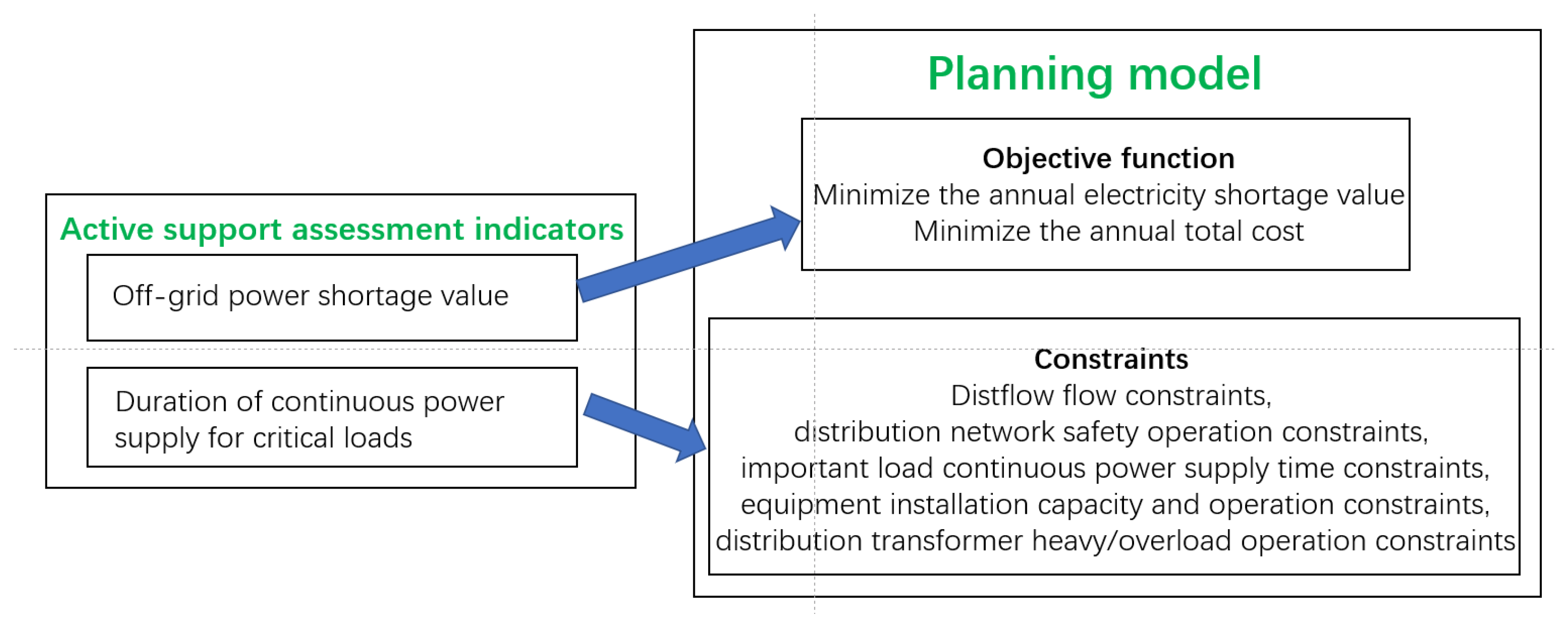
This section introduces the optimization objectives together with the associated operational constraints for device deployment. By simultaneously accounting for economic efficiency and active support capability during islanded operation, a joint planning framework integrating flexible interconnection devices and GFM-ESSs is established, as depicted in Figure 1.

2.1. Objective Function

The planning problem contains both long-horizon equipment investment and short-horizon operation under off-grid faults. Therefore, a hierarchical structure is adopted. The upper layer selects the locations and capacities of flexible interconnection devices, GFM-ESSs and DC lines, while the lower layer checks operational feasibility and quantifies active support effects during islanded fault scenarios. Compared with a single-layer formulation, this structure more clearly links planning decisions with post-fault power exchange, load supply, voltage security and critical-load support.

Two optimization goals are considered in this study: reducing the equivalent annual total expenditure and decreasing the yearly power deficit caused by system faults.

$$\left\{\begin{array}{l}\min F_1=C_{inv}^S+C_o\\ \min F_2=365{\displaystyle \sum _{t=1}^{T_{\max }}{\displaystyle \sum _{i\in N_{\mathrm{DN}}}{P}_{load,i,t}\mathrm{\Delta }t}}\end{array}\right.$$

(1)

where $C_{inv}^S$ represents the annualized investment expenditure associated with VSCs, GFM-ESS units, and DC lines, while $C_o$ denotes the yearly operation and maintenance expenses of the distribution network.

$$C_{inv}^S={\displaystyle {\displaystyle \sum _{i=1}^{N_{VSC}}}{\alpha }_{VSC}{C}_{VSC}{S}_{VSC,i}}+{\displaystyle {\displaystyle \sum _{j=1}^{N_{ESS}}}{\alpha }_{ESS}{C}_{ESS}{S}_{ESS,j}}+{\alpha }_L{C}_L{L}_{DC}+{\alpha }_{DB}{C}_{DB}{N}_{DB}$$

(2)

In Equation (2), $C_{VSC}$ and $C_{ESS}$ denote the per-unit capacity investment coefficients for VSCs and ESSs, respectively; $N_{VSC},N_{ESS}$ are the numbers of installed VSCs and ESSs; $C_L$ is the DC-line unit-length cost; and $C_{DB}$ represents the expenditure associated with each distribution box. $S_{VSC,i}$ and $S_{ESS,j}$ are the installed capacities at the corresponding candidate sites; $L_{DC}$ is the total DC-line length; and $N_{DB}$ denotes the number of additional distribution boxes deployed. The coefficients ${\alpha }_{VSC},{\alpha }_{ESS},{\alpha }_L,{\alpha }_{DB}$ convert the one-time investments into equivalent annual costs, which can be expressed by Equation (3).

$$\alpha ={\displaystyle \frac{r{(1+r)}^Y}{{(1+r)}^Y-1}}$$

(3)

In Equation (3), $r$ denotes the discount factor, while $Y$ corresponds to the service lifetime, namely, the depreciation horizon, of the equipment.

The operation-and-maintenance cost is modeled by considering line losses, device operation, inspection and maintenance, and load shedding. Differences in maintenance requirements among newly installed devices at different locations are also included.

$$C_o=C_{loss}+C_{device}+C_{service}+C_{load}$$

(4)

In Equation (4), $C_{loss}$ refers to the yearly expense caused by network power losses; $C_{device}$ represents the operating expenditures of VSCs and ESSs; $C_{service}$ is the inspection and maintenance cost of these devices; and $C_{load}$ is the cost associated with curtailed load.

$$C_{loss}=365{\displaystyle \sum _{t=1}^{T_{\max }}{C}_e\left({\displaystyle \sum _{l\in {\mathrm{\Omega }}_{AC,line}}{P}_{AC,L,t,l}}+{\displaystyle \sum _{l\in {\mathrm{\Omega }}_{DC,line}}{P}_{DC,L,t,l}}\right)}\mathrm{\Delta }t$$

(5)

In Equation (5), $C_e$ represents the electricity tariff that varies over time. $P_{AC,L,t,l}$ and $P_{DC,L,t,l}$ describe the power losses of line l at time t in the AC and DC subsystems, respectively, while ${\mathrm{\Omega }}_{AC,line}$ and ${\mathrm{\Omega }}_{DC,line}$ denote the corresponding AC and DC line sets.

$$C_{device}=365{\displaystyle \sum _{t=1}^{T_{\max }}\left(a_{VSC,i}{\displaystyle {\displaystyle \sum _{i=1}^{N_{VSC}}}{P}_{VSC,t,i}}+a_{ESS,j}{\displaystyle {\displaystyle \sum _{j=1}^{N_{ESS}}}{P}_{ESS,t,j}}\right)}\mathrm{\Delta }t$$

(6)

In Equation (6), $a_{VSC,i}$ and $a_{ESS,j}$ are the unit operating costs of the VSC and ESS at their installation sites, and $P_{VSC,t,i}$ and $P_{ESS,t,j}$ are their active power outputs at time t.

$$C_{service}=C_{ESS}^{ser}+C_{VSC}^{ser}+C_{ESS}^{vender}+C_{VSC}^{vender}$$

(7)

$$C_{load}=365C_l{\displaystyle \sum _{t=1}^{T_{\max }}{\displaystyle \sum _{i\in {\mathrm{\Omega }}_{load,t}}{P}_{in,t,i}\mathrm{\Delta }t}}$$

(8)

In Equation (8), $C_l$ is the unit penalty for load curtailment, $P_{in,t,i}$ represents the active demand at node $i$ during time period $t$, and ${\mathrm{\Omega }}_{load,t}$ identifies the collection of nodes experiencing load shedding in that interval.

2.2. Constraint Condition

(1)

DistFlow equation equality constraint

Because the voltage phase-angle variation along low-voltage AC branches is relatively small, the DistFlow model is employed to characterize the network power flow behavior. This representation neglects phase-angle variables and retains voltage magnitudes, which reduces model complexity and shortens the solution time. The adopted equations are given below:

$$\left\{\begin{array}{c}{\displaystyle \sum _{k\in L_s}{P}_{jk,t}}-{\displaystyle \sum _{i\in L_t}\left(P_{ij,t}-I_{ij,t}^2{r}_{ij}\right)=P_{j,t}^{PV}+P_{j,t}^{ESS}+P_{j,t}^{VSC}-P_{j,t}^{load}}\hfill \\ {\displaystyle \sum _{k\in L_s}{Q}_{jk,t}}-{\displaystyle \sum _{i\in L_t}\left(Q_{ij,t}-I_{ij,t}^2{x}_{ij}\right)=Q_{j,t}^{PV}+Q_{j,t}^{ESS}+Q_{j,t}^{VSC}-Q_{j,t}^{load}}\hfill \end{array}\right.$$

(9)

$$U_{j,t}^2=U_{i,t}^2-2(r_{ij}{P}_{ij,t}+x_{ij}{Q}_{ij,t})+(r_{ij}^2+x_{ij}^2)I_{ij,t}^2$$

(10)

$$I_{ij,t}^2={\displaystyle \frac{P_{ij,t}^2+Q_{ij,t}^2}{U_{i,t}^2}}$$

(11)

In Equations (9)–(11), $L_s$ and $L_t$ denote the sets of branches ending at nodes i and j. $P_{ij,t}$ and $Q_{ij,t}$ represent the active and reactive power transmitted through branch ij at time interval t; $r_{ij}$ and $x_{ij}$ are its resistance and reactance; and $I_{ij,t}$ is the branch current. $P_{j,t}^{PV}$ and $Q_{j,t}^{PV}$ are the photovoltaic outputs; $P_{j,t}^{ESS}$ and $Q_{j,t}^{ESS}$ are the powers injected by ESS; $P_{j,t}^{VSC}$ and $Q_{j,t}^{VSC}$ are the VSC injections; $P_{j,t}^{load}$ and $Q_{j,t}^{load}$ are the load demands; and $U_{i,t}$ and $U_{j,t}$ denote the voltage amplitudes at nodes i and j, respectively.

(2)

Distribution network safety operation constraints

All node voltages in the LVDN must stay within their permissible bounds. For the low-voltage network considered in this study, the acceptable voltage interval is defined as 0.93–1.07 p.u. Moreover, the current flowing through each branch must remain below its thermal carrying capability, resulting in the following constraint set.

$$\left\{\begin{array}{c}{U}_{i,\min }\le U_i\le U_{i,\max }\\ I_{i,j\min }\le I_{ij,t}\le I_{ij,\max }\end{array}\right.$$

(12)

In the expression: $U_{i,\max }$ and $U_{i,\max }$ denote the minimum and maximum allowable voltage magnitudes at node $i$, respectively, while $I_{i,j\min }$ and $I_{ij,\max }$ represent the corresponding lower and upper current bounds for branch ij.

(3)

Constraint on uninterrupted supply duration for critical loads during islanded operation

$$T_{\max }^{loadn}\ge T_{\mathrm{expect}}^n$$

(13)

The parameter $T_{\mathrm{expect}}^n$ specifies the minimum islanded operation duration required by the decision-maker for the nth critical load.

(4)

Installation capacity constraint of new equipment

$$\left\{\begin{array}{l}{x}_i^{ESS}{E}_{ESS,\min }\le E_{ESS,i}\le x_i^{ESS}{E}_{ESS,\max }\\ x_i^{VSC}{E}_{VSC,\min }\le E_{VSC,i}\le x_i^{VSC}{E}_{VSC,\max }\end{array}\right.$$

(14)

In Equation (14), $x_i^{ESS}$ and $x_i^{VSC}$ are binary siting variables indicating whether a GFM-ESS or VSC is installed at node i. $E_{ESS,\max }$ and $E_{ESS,\min }$ bound the GFM-ESS capacity, and $E_{VSC,\max }$ and $E_{VSC,\max }$ bound the VSC capacity.

(5)

Load distribution/overload operation constraints

Flexible DC interconnections allow transformer areas to exchange energy and relieve heavy loading on distribution transformers. Accordingly, once flexible interconnection is activated, the operating conditions of the distribution transformer should comply with the following limits.

$$P^L(t)\ge 0$$

(15)

$$\sqrt{P^H{(t)}^2+Q^H{(t)}^2}\le 0.7S_T$$

(16)

In Equations (15) and (16), $P^L(t)$ denotes the active power measured at the low-voltage side of the transformer. $P^H(t)$ and $Q^H(t)$ correspond to the active and reactive power quantities on the high-voltage side, respectively, and $S_T$ represents the rated apparent-power capacity of the transformer.

(6)

Power transfer constraints of flexible interconnection

During VSC operation, power conservation must be maintained between the AC and DC terminals, meaning that the active power absorbed from the AC side must equal the power transferred to the DC side. Meanwhile, both the active and reactive power outputs of the VSC are constrained by its rated converter capacity, as formulated below.

$$P_{VSC,t}^{AC}=-P_{VSC,t}^{DC}$$

(17)

$${P_{VSC,t}^{AC}}^2+{Q_{VSC,t}^{AC}}^2\le S_{VSC}^2$$

(18)

In Equations (17) and (18), $P_{VSC,t}^{AC}$ and $Q_{VSC,t}^{AC}$ are the VSC active and reactive powers on the AC side at time t, $P_{VSC,t}^{DC}$ is the DC-side active power, and $S_{VSC}$ denotes the rated VSC capacity.

(7)

Power transfer constraints for energy storage devices

For ESS operation, the charging and discharging powers are first limited by their rated power bounds. The state of charge then evolves according to the charge/discharge process. To extend battery life, SOC is restricted to the 20–80% range. Furthermore, consistency is imposed between the initial and final SOC values within each daily scheduling horizon.

$$\left\{\begin{array}{l}0\le P_{ESSch}\left(t\right)\le P_{ESSch,\max }\\ 0\le P_{ESSdis}\left(t\right)\le P_{ESSdis,\max }\end{array}\right.$$

(19)

$$SO{C}_{ESS}\left(t\right)=SO{C}_{ESS}\left(t-1\right)+SO{C}_{ESS}\left(\mathrm{\Delta }t\right)$$

(20)

$$SO{C}_{ESS}\left(\mathrm{\Delta }t\right)=\left\{\begin{array}{l}{\lambda }_1{P}_{ESSch}\left(t\right){\eta }_{ESSch}\mathrm{\Delta }t\\ {\lambda }_2{\displaystyle \frac{-P_{ESSdis}\left(t\right)\mathrm{\Delta }t}{{\eta }_{ESSdis}}}\end{array}\right.$$

(21)

$${\lambda }_1+{\lambda }_2\le 1,\forall t$$

(22)

$$SO{C}_{ESS\min }\le SO{C}_{ESS}\left(t\right)\le SO{C}_{ESS\max }$$

(23)

$$SO{C}_{ESS,j,T\mathrm{bejin}}=SO{C}_{ESS,j,Tfinish}$$

(24)

In Equations (19)–(24), $P_{ESSch}\left(t\right)$ and $P_{ESSdis}\left(t\right)$ denote charging and discharging powers; and $P_{ESSch,\max }$ and $P_{ESSdis,\max }$ specify their corresponding upper bounds. $SO{C}_{ESS}\left(t\right)$ and $SO{C}_{ESS}\left(t-1\right)$ are the storage states at two consecutive time steps; $SO{C}_{ESS}\left(\mathrm{\Delta }t\right)$ is the SOC variation in period t; the variables ${\lambda }_1$ and ${\lambda }_2$ are binary indicators corresponding to charging and discharging modes, respectively; ${\eta }_{ESSch}$ and ${\eta }_{ESSdis}$ are efficiencies; $SO{C}_{ESS\min }$ and $SO{C}_{ESS\max }$ define the SOC bounds; and $SO{C}_{ESS,j,T\mathrm{bejin}}$ and $SO{C}_{ESS,j,Tfinish}$ are the initial and terminal SOC values for daily scheduling at node j.

3. Evaluation Method for the Active Supporting Effect of the Grid Planning Scheme

3.1. Evaluation Indicators of Active Support Evaluation

Active support is defined as the capability of grid-forming equipment to build stable voltage and frequency references and to maintain LVDN load supply when the upstream grid fails. Based on this definition, the following evaluation indices are constructed.

(1)

Off-grid power shortage value

Energy not supplied (ENS) measures the accumulated load shortage during islanded operation of a representative transformer area over a typical day. It is computed as follows.

$$ENS={\displaystyle \sum _{t=1}^{T_{\max }}{\displaystyle \sum _{i\in N_{\mathrm{DN}}}{P}_{load,i,t}\mathrm{\Delta }t}}$$

(25)

In Equation (25), $T_{\max }$ denotes the total number of scheduling periods, which is specified as 24 h in this work. $N_{\mathrm{DN}}$ represents the set of nodes in the distribution network, $P_{load,i,t}$ corresponds to the curtailed load at node i during time interval t, and $\mathrm{\Delta }t$ denotes the length of each scheduling step.

(2)

Sustained supply duration of critical loads during islanded operation

The sustained supply duration of critical loads characterizes the length of time for which all important loads can remain energized under a typical islanded operating scenario. This performance index is calculated using Equation (26).

$$T_{keep}=\min (T_{\max }^{load1},T_{\max }^{load2},\mathrm{\dots },T_{\max }^{loadn})$$

(26)

In the expression: $T_{\max }^{loadn}$ denotes the maximum uninterrupted supply duration available to the nth critical load within the islanded operation of the corresponding substation area.

As defined in Equation (26), this parameter reflects the duration for which the nth important load can be continuously supported when the transformer area operates in off-grid mode.

Together, ENS and the sustained supply duration of critical loads provide a concise set of indicators for assessing the active support capability of different planning schemes.

3.2. Comprehensive Assessment Method for Active Support Effect

In order to analyze the effect of various flexible interconnection and GFM-ESS configuration schemes on improving active support capability, a comprehensive evaluation method of the active support effect is proposed, and based on the established active support capability evaluation index, the comprehensive evaluation value of the active support effect is obtained by normalization and the subjective weighting method.

Because the two active support indices have different units and scales, they must be transformed into dimensionless values. The normalization formula is given below:

$${r_i}^{\prime }={\displaystyle \frac{r_i-\min r_i}{\max r_i-\min r_i}}$$

(27)

In Equation (27), $r_i$ is the original value of the ith indicator, ${r_i}^{\prime }$ is its normalized value; and $\max r_i$ and $\min r_i$ are the maximum and minimum values of that indicator.

Since only two indicators are used, subjective weights are assigned to the normalized variables, and the integrated evaluation value $Com$ is obtained using Equation (28).

$$Com={\displaystyle \sum _{i=1}^n{w}_i\times {r_i}^{\prime }}$$

(28)

In Equation (28), $w_i$ represents the weight assigned to the ith evaluation indicator.

By combining the normalized indices and their weights, the comprehensive active support score is obtained as Equation (29). A smaller score indicates a better support effect.

$$Effect=w_{ENS}\times {r_{ENS}}^{\prime }-w_T\times {r_T}^{\prime }$$

(29)

In Equation (29), $w_{ENS}$ and $w_T$ are the weights of the ENS and critical-load supply-duration indices, while ${r_{ENS}}^{\prime }$ and ${r_T}^{\prime }$ are their normalized values.

This section builds an active support effect evaluation method based on the planning scheme, verifies and evaluates the actual support ability of the planning scheme when dealing with off-grid scenarios through quantitative indicators, and forms a complete technical closed loop of “planning modeling-effect verification”.

4. Solution Method of the Model

To avoid the local-optimum risk and low efficiency of heuristic algorithms such as genetic algorithms, the nonconvex nonlinear model is solved through SOCP. This approach improves computational efficiency while retaining global optimality after valid convex relaxation. The optimization model is implemented in MATLAB (R2024a) using YALMIP toolbox (R2023) and solved with Gurobi (v11.0).

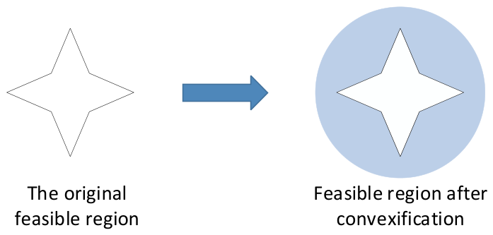
The proposed planning model is relaxed using second-order cone convexification. The nonconvex terms are mainly associated with Equations (9)–(11), and the relaxation principle is shown in Figure 2.

Define the cone optimization variables $l_{ij,t}$ and $l_{ij,t}$. Let $v_{i,t}=U_{i,t}^2$, $l_{ij,t}=I_{ij,t}^2$. Then, we have: $l_{ij,t}{v}_{i,t}\ge P_{ij,t}^2+Q_{ij,t}^2$. After the relaxation process, Equations (9)–(11) are transformed into Equation (30).

$$\left\{\begin{array}{l}{\displaystyle \sum _{k\in L_s}{P}_{jk,t}}-{\displaystyle \sum _{i\in L_t}\left(P_{ij,t}-l_{ij,t}{r}_{ij}\right)=P_{j,t}^{PV}+P_{j,t}^{ESS}+P_{j,t}^{VSC}-P_{j,t}^{load}}\hfill \\ {\displaystyle \sum _{k\in L_s}{Q}_{jk,t}}-{\displaystyle \sum _{i\in L_t}\left(Q_{ij,t}-l_{ij,t}{x}_{ij}\right)=Q_{j,t}^{PV}+Q_{j,t}^{ESS}+Q_{j,t}^{VSC}-Q_{j,t}^{load}}\hfill \\ v_{j,t}=v_{i,t}-2(r_{ij}{P}_{ij,t}+x_{ij}{Q}_{ij,t})+(r_{ij}^2+x_{ij}^2)l_{ij,t}\hfill \\ l_{ij,t}{v}_{i,t}\ge P_{ij,t}^2+Q_{ij,t}^2\hfill \end{array}\right.$$

(30)

Then, the annual fault capacity shortage value of objective function 2 is converted into cost, as shown in Equation (31). Finally, the dual-objective function is converted into a single-objective function, and the optimal planning scheme is solved by the linear programming method.

$$\min F_2=365C_e{\displaystyle \sum _{t=1}^{T_{\max }}{\displaystyle \sum _{i\in N_{\mathrm{DN}}}{P}_{load,i,t}\mathrm{\Delta }t}}$$

(31)

In the expression: $C_e$ represents the real-time electricity price.

5. Example Analysis

5.1. Background

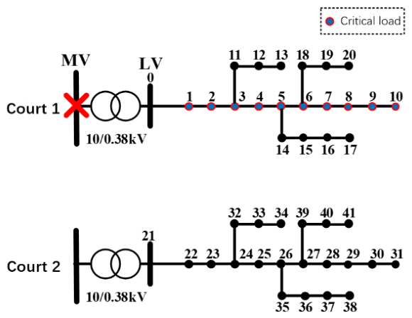
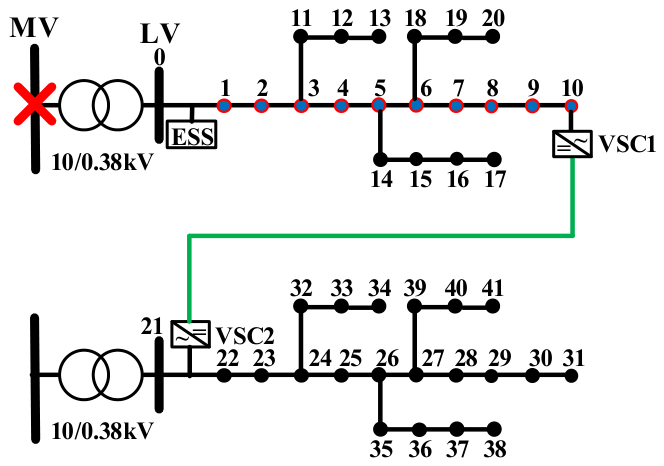
Assuming that an upstream-grid fault occurs in Zone 1, resulting in a power interruption within the low-voltage distribution system, as shown in Figure 3, the outage duration is set from 17:45 to 19:45. The transformer capacities in both Zone 1 and Zone 2 are specified as 0.25 MVA.

5.2. Validation Analysis of the Planning Method

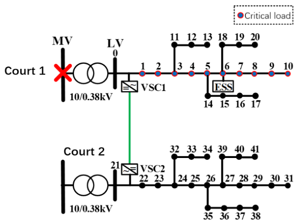
Using the SOCP approach, the optimal siting results are obtained and presented in Figure 4. The GFM-ESS is installed at node 6 with a rated capacity of 331 kWh, while VSC units with a capacity of 58 kVA are deployed at nodes 0 and 21. In addition, the total length of the DC interconnection line is determined to be 0.4 km.

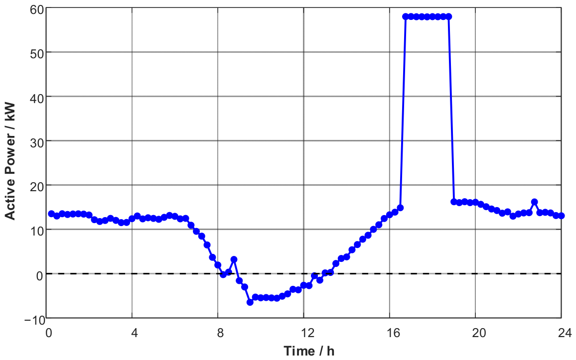
The power curve of VSC2 during the fault period is shown in Figure 5. Subject to the non-overload constraint of the transformer in Area 2, VSC2 transfers as much available power as possible from Area 2 to Area 1. This reduces the power burden on the GFM-ESS and lowers the required storage capacity. Since the unit investment cost of the VSC capacity is relatively low, the resulting scheme also maintains good economic performance.

To evaluate the effectiveness of the proposed strategy, three planning schemes are compared. Scheme 1 installs only GFM-ESSs, Scheme 2 adopts the proposed coordinated planning strategy, and Scheme 3 installs only flexible interconnection devices. The results are reported in

Table 1. Results of different planning methods.

Scheme	Annual Investment Cost/Ten Thousand Yuan	Annual Operation and Maintenance Cost/Ten Thousand Yuan	Annual Comprehensive Cost/Ten Thousand Yuan	Every Year ENS/MWh
1	25.97	2.26	28.23	0
2	21.01	2.14	23.15	0

Annual investment cost is calculated according to Equations (2) and (3). Annual operation and maintenance cost is based on Equation (4). Annual comprehensive cost is the sum of the annual investment cost and the annual operation and maintenance cost.

. Scheme 3 is infeasible because it cannot simultaneously satisfy the required critical-load supply duration and the loading constraints of transformer 2.

Table 1 indicates that both feasible schemes can improve the active support capability of the LVDN, whereas the coordinated planning scheme shows better economic performance. This advantage is mainly attributed to the relatively high unit capacity investment cost of GFM-ESSs, which leads to a higher annual comprehensive cost when only energy storage is deployed. In contrast, VSC-based flexible interconnection devices can redistribute surplus power from the unaffected transformer area to the faulted region. Consequently, the discharge burden on the GFM-ESS during upstream-grid outages is reduced, allowing for a smaller installed ESS capacity and a more cost-effective overall solution.

5.3. Analysis of the Impact of Flexible Interconnection Capacity on Active Support Performance

The capacity of flexible interconnections has varying impacts on the active support performance of the LVDN. The specific effects of changes in the flexible interconnection capacity on the active support performance are analyzed as follows.

(1)

Impact of Flexible Interconnection Device Capacity on Active Support Performance

First, the integration point of VSC1 is set at Node 5, and the integration point of VSC2 is set at Node 21, with these locations kept constant. This placement scheme ensures that there are no voltage limit violations in either distribution zone 1 or distribution zone 2.

Next, the capacity of the VSCs is varied to analyze the corresponding changes in each active support evaluation index.

Finally, the variation of the comprehensive active support evaluation value with respect to the VSC capacity is analyzed. It is assumed that the transformer capacity in distribution zone 2 is sufficiently large to support the normal operation of VSCs of any capacity.

The values of the active support evaluation indices under typical capacities are presented in

Table 2. Evaluation index values under typical VSC capacities.

VSC Capacity/kVA	ENS/kWh	Tkeep/h
58	233.31	0.5
65	201.9	1
76	130.83	2
151	0	2
200	0	2

.

After normalizing the evaluation index values from the above table, the resulting evaluation values are shown in

Table 3. Normalized evaluation index values.

VSC Capacity/kVA	ENS	Tkeep
58	1	0
65	0.865	0.333
76	0.561	1
151	0	1
200	0	1

.

(2)

Sensitivity Analysis of the Impact of Flexible Interconnection Capacity on Active Support Performance

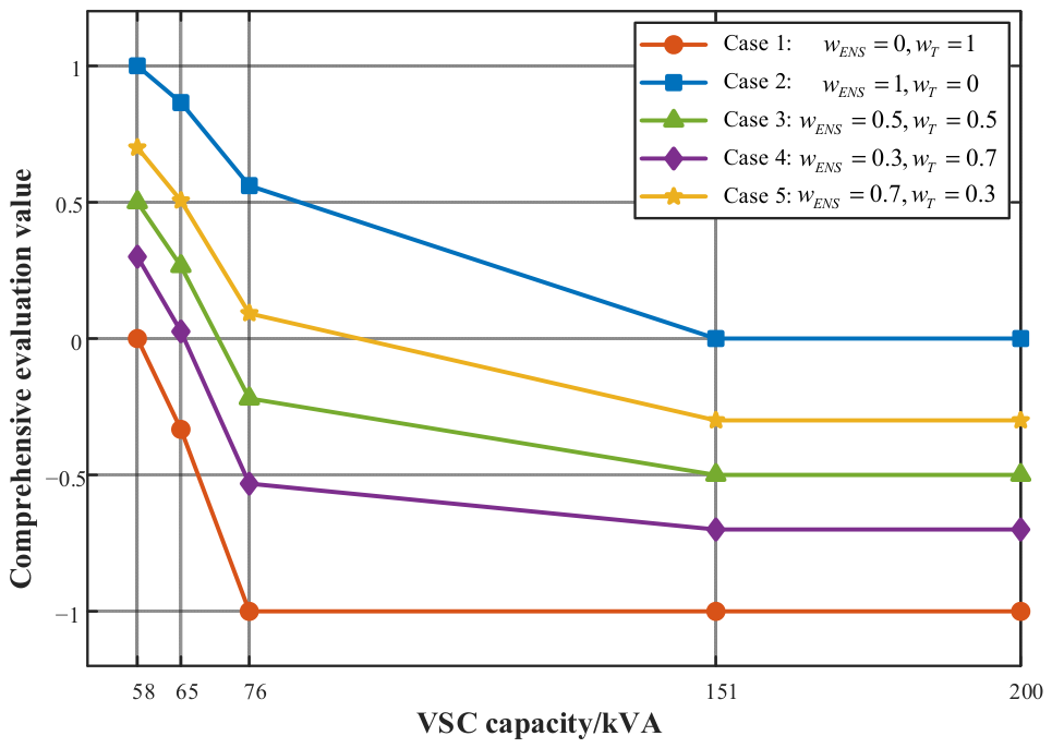
To comprehensively analyze the impact of the flexible interconnection VSC capacity on the active support performance under different evaluation preferences, five sets of evaluation index weight combinations are established for sensitivity analysis. Here, $w_{ENS}$ is the weight of the ENS index, and $w_T$ is the weight assigned to the continuous supply time of critical loads. The five sets of weights in the figure (0 and 1, 1 and 0, 0.5 and 0.5, 0.3 and 0.7, and 0.7 and 0.3, respectively) represent the varying degrees of emphasis decision-makers place on the two dimensions of “reducing energy shortage” and “extending continuous power supply time for critical loads” during the comprehensive evaluation process. The analysis results indicate that despite the different weight distributions, the overall variation trends of all curves are highly consistent.

The finally obtained variation curves of the comprehensive active support evaluation value with respect to the VSC capacity are shown in Figure 6.

Figure 6 indicates that the comprehensive evaluation score decreases as the VSC capacity increases, which means that the active support effect improves. The trend can be divided into three stages.

• When the VSC capacity is less than 76 kVA: The comprehensive evaluation value decreases rapidly with the increase in VSC capacity. This is because the baseline VSC capacity is small; so, an increase in capacity has a highly significant impact on active support. Both the ENS index and the continuous power supply time for the critical-loads index are substantially improved.
• When the VSC capacity is between 76 kVA and 151 kVA: The rate of decline in the comprehensive evaluation value noticeably slows down as the VSC capacity increases. This is because the index for the continuous power supply time for critical loads has already reached its optimal state within this VSC capacity range and remains constant. At this stage, the optimization of the comprehensive evaluation value is driven solely by the continuous reduction of the ENS index value, resulting in a slower decline.
• When the VSC capacity is greater than 151 kVA: A VSC capacity of 151 kVA is exactly sufficient to meet the power requirement at the moment of the maximum total load power demand under the fault scenario. When the VSC capacity exceeds 151 kVA, the comprehensive evaluation value reaches its optimum and remains constant. This is because both evaluation index values have achieved their optimal states and remain constant within this capacity range. Since the VSC itself does not possess energy storage capabilities, its active support effect—exerted through spatial power transfer—achieves its optimum when the VSC capacity is precisely sufficient to meet the power requirement at the moment of the maximum total load demand under the fault scenario.

5.4. Analysis of the Impact of Coordinated Configuration of Flexible Interconnection and Grid-Type Energy Storage on Active Support Effect

Flexible interconnection and GFM-ESSs have a different influence on the active support effect of the LVDN. The influence of equipment’s access position and capacity on the active support effect is analyzed respectively.

(1)

Influence of equipment capacity on active support effect

Under the condition that the equipment access position is unchanged, the active support effect reaches the optimum when the VSC capacity is just enough to meet the power of the maximum time of the total load power demand under the fault scenario, and the active support effect reaches the optimum when the GFM-ESS capacity is just enough to meet the total load power demand under the fault scenario.

(2)

Influence of equipment access position on active support effect

First, the capacities of GFM-ESS and VSC are set to 330 kWh and 58 kVA, respectively, and their capacities are kept unchanged. Then, the connection positions of GFM-ESS and VSC are changed, and the changes in each active support evaluation index and the influence of the voltage over-limit problem are analyzed. Since the voltage over-limit probability is low when VSC is connected at the head end of the non-fault station area, the VSC of the non-fault station area is suitable to be connected at the position close to the head end node; so, VSC2 is connected at node 21, and its position is kept unchanged. The evaluation index values obtained by solving and the line loss values of substation area 1 are shown in

Table A2. Evaluation indicators and line loss results for VSC and ess at different access locations.

Topological Numbering	VSC1 Position	ESS Position	ENS/kWh	Tkeep/h	Line Loss of the Transformer Area 1/kWh
1	0	1	15.24	2	9.74
3	0	2	10.21	2	6.88
3	0	3	5.84	2	4.39
4	0	4	3.22	2	2.89
5	0	5	1.07	2	1.66
6	0	6	0.90	2	1.57
7	0	7	2.30	2	2.37
8	0	8	4.16	2	3.43
9	0	9	6.49	2	4.76
10	0	10	9.33	2	6.37
11	5	0	10.18	2	6.86
12	5	1	6.90	2	4.99
13	5	2	4.16	2	3.43
14	5	3	1.91	2	2.14
15	5	4	1.27	2	1.78
16	5	5	1.05	2	1.65
17	5	6	0.88	2	1.56
18	5	7	2.30	2	2.36
19	5	8	4.16	2	3.43
20	5	9	6.50	2	4.76
21	5	10	9.35	2	6.38
22	10	0	9.84	2	6.66
23	10	1	6.59	2	4.81
24	10	2	3.87	2	3.26
25	10	3	1.63	2	1.99
26	10	4	1.00	2	1.63
27	10	5	0.79	2	1.51
28	10	6	2.55	2	2.51
29	10	7	5.97	2	4.46
30	10	8	9.94	2	6.72
31	10	9	14.54	2	9.34
32	10	10	19.81	2	12.35
33	0	0	20.99	2	13.02

. It can be seen that when VSC1 and GFM-ESS are connected to head-end node 0 and terminal node 10 at the same time, the voltage in substation area 1 will exceed the limit, which does not meet the constraint conditions for safe operation of the distribution network. Therefore, active support effect analysis for these two topologies is not performed.

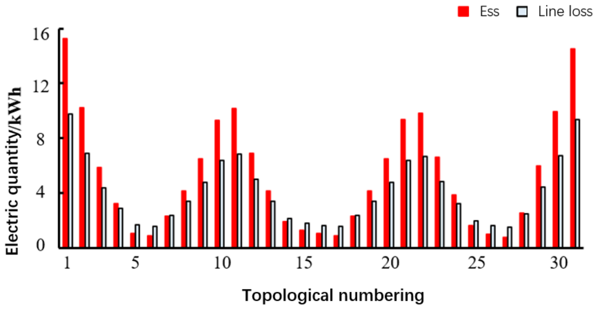
Table A2 shows that the critical-load continuous supply time is 2 h for the tested schemes. Therefore, comparing only the ENS values can determine which topology provides the best active support effect. Since the ENS value of topology 27 is the smallest, the active support effect of topology 27 is the best. In addition, the topologies with the ENS value close to the smallest include topology 6 and topology 17. Although the access position of VSC1 is different, the access position of GFM-ESS in these two topologies is node 6, which is very close to intermediate node 5. According to Figure 7, when the location of VSC1 remains unchanged, the ENS value shows a variation trend consistent with the line loss in station area 1. The minimum ENS is obtained when the GFM-ESS is connected to an intermediate node. Therefore, under the given capacities of the GFM-ESS and VSC, placing the GFM-ESS at an intermediate node can achieve the best active support effect.

As shown in Figure 7, the ENS index value is consistent with the trend of line total loss value in station 1. The larger the line loss value in station 1, the larger the ENS index value. Different equipment access positions lead to changes in the LVDV power flow, resulting in changes in the line loss. The larger the line total loss, the higher the power demand on GFM-ESS. However, the capacity of GFM-ESS is limited, resulting in a larger ENS. Therefore, when the network equipment only changes its position, the ENS value theoretically depends on the line loss of the lost station area during the fault period, and the ENS evaluation index is positively correlated with the line loss of the lost station area during the fault period.

To further identify the optimal locations of GFM-ESS and VSC1 for active support enhancement, a refined location analysis is conducted for VSC1. In the previous analysis, only three representative VSC1 locations, namely, the head-end node 0, the intermediate node 5, and the terminal node 10, were considered. Therefore, this section further investigates the active support performance under different VSC1 locations when GFM-ESS is connected to node 5 or node 6. The corresponding results are listed in

Table A3. Evaluation index values of VSC1 at different positions.

ESS Position	VSC1 Position	ENS/kWh	Tkeep/h
5	0	1.07	2
5	1	0.62	2
5	2	0.31	2
5	3	0.13	2
5	4	0.52	2
5	5	1.05	2
5	6	0.38	2
5	7	0.27	2
5	8	0.31	2
5	9	0.48	2
5	10	0.79	2
6	0	0.90	2
6	1	0.30	2
6	2	0.01	2
6	3	0	2
6	4	0.24	2
6	5	0.88	2
6	6	2.13	2
6	7	2.03	2
6	8	2.07	2
6	9	2.24	2
6	10	2.55	2

.

As shown in Table A3, the minimum ENS is obtained when GFM-ESS is installed at node 6 and VSC1 is connected to node 3, indicating that this configuration provides the best active support performance.

By comparing Table A2 with Table A3, it can be observed that the variation in ENS caused by changing the GFM-ESS location is approximately 14 kWh, whereas the ENS variation resulting from different VSC1 locations is only about 2.5 kWh. This indicates that the siting of GFM-ESS has a more significant impact on active support performance than that of VSC1. The main reason is that GFM-ESS delivers 329.17 kWh during the upstream-grid fault period, while VSC1 provides only 74.61 kWh. Since GFM-ESS contributes more energy support, its location has a stronger influence on the power flow distribution and line losses. Accordingly, the GFM-ESS installation position plays a more dominant role in determining the active support performance.

In summary, when the capacities of the VSC and GFM-ESS remain unchanged, the location of the GFM-ESS has a greater impact on active support performance if the GFM-ESS provides stronger power support to the faulted transformer area than the VSC. Therefore, installing the GFM-ESS at an intermediate node is more suitable for improving the active support effect.

5.5. Analysis of Advantages of Flexible Interconnection and Network Energy Storage Coordination Planning

(1)

Active support effect and economy

From the active support effect level, the flexible interconnection and GFM-ESS coordination planning will inevitably make the active support effect optimal, and at the same time can improve the shortcomings of only configuring flexible interconnection devices in the active support effect, because GFM-ESS has the ability to construct a network, can store energy, and does not depend on the power transfer of the interconnection area.

From the economic level, on the premise of ensuring the active support effect, flexible interconnection and GFM-ESS coordination planning can optimize the economy and improve the high investment cost of GFM-ESS, because compared with GFM-ESS, VSC is cheaper, and flexible interconnection can reduce the capacity allocation of GFM-ESS.

(2)

Improvement of power quality issues

From the perspective of power quality, the joint planning of VSC-based flexible interconnection devices and GFM-ESSs can more effectively mitigate voltage limit violations. If a GFM-ESS is deployed alone, an unsuitable installation location may cause bus voltages to exceed their allowable range. Similarly, when only flexible interconnection devices are installed, improper siting may also lead to unacceptable voltage deviations. Coordinated planning enables the two resources to complement each other in voltage regulation and fault support. Moreover, the power transfer function of VSC-based interconnections helps share part of the load demand during faults, thereby lowering the storage capacity that must be installed.

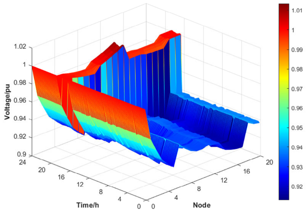
Figure 8 presents the network configuration incorporating flexible interconnection devices together with a GFM-ESS. Based on the preceding case analysis, it can be observed that deploying only a GFM-ESS at node 0 causes undervoltage issues near the feeder terminal, whereas relying solely on flexible interconnection devices results in a voltage deficiency around the feeder head of Station 1. Under the proposed optimization framework, the installation locations of the VSC and GFM-ESS remain fixed, while their rated capacities are selected as the key decision variables. The corresponding voltage profiles are presented in Figure 9.

Figure 9 demonstrates that, under the off-grid operating condition, the bus voltages in station area 1 remain within the permissible range. In particular, the undervoltage issue near the feeder terminal is effectively mitigated. These findings confirm that the joint optimization of flexible interconnection devices and a GFM-ESS enhances the voltage regulation capability and effectively mitigates voltage limit violations.

5.6. Multi-Representative-Day Scenario Setting

To further evaluate the robustness and practical applicability of the developed planning framework, an additional representative-day scenario is considered. Scenario 2 represents a high-load and low-PV-output day, where the evening peak load is increased and photovoltaic generation is reduced compared with the base scenario.

Both scenarios are simulated over a 24 h scheduling horizon. The network topology, transformer ratings, candidate device locations, device capacities and fault location are kept the same. The upstream-grid fault is imposed on Zone 1 during the evening peak period; so, the comparison focuses on whether the proposed scheme remains robust under different operating conditions.

Compared with Scenario 1, Scenario 2 creates a heavier supply burden in the faulted area because the evening peak load is higher and the PV output is lower. Therefore, both the VSC transfer requirement and the GFM-ESS output demand increase to some extent. Nevertheless, the coordinated planning scheme can still maintain critical-load supply and voltage security during the off-grid period.

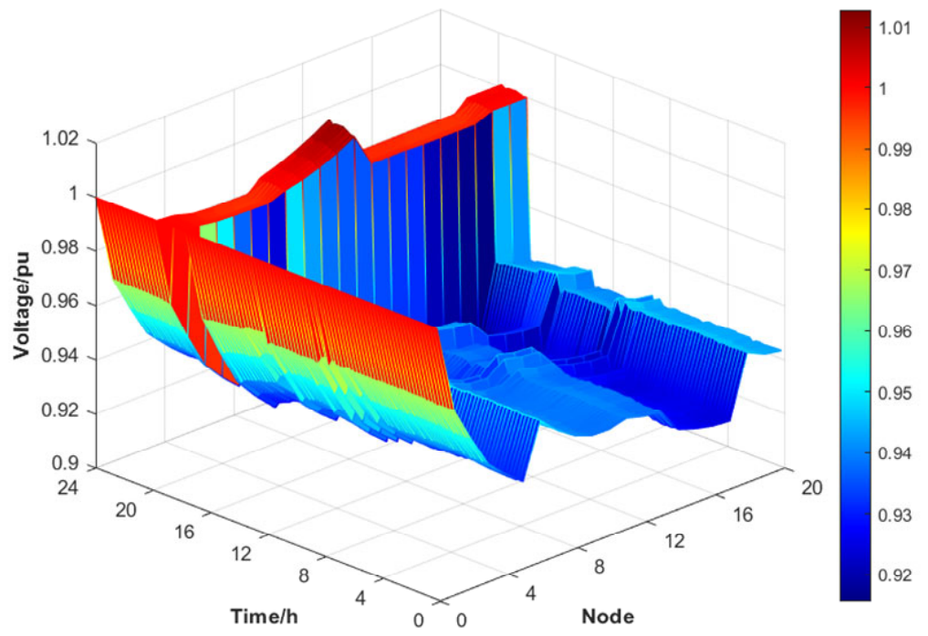
Figure 10 presents the voltage distribution of Zone 1 over time and across different nodes under Scenario 2. It can be found that the voltage magnitudes are mainly kept between 0.93 and 1.01 p.u. over the daily operation horizon, meeting the voltage security limits of the LVDN. Due to changes in load demand, PV generation, and the supply pattern after the upstream-grid fault, several buses, especially those close to the feeder terminal, experience a voltage decline during certain intervals. The lowest voltage level appears around the evening peak fault period. However, the coordinated operation of the flexible interconnection device and GFM-ESS keeps all bus voltages within the allowable range, indicating that the proposed planning method is effective in supporting secure and feasible off-grid operation.

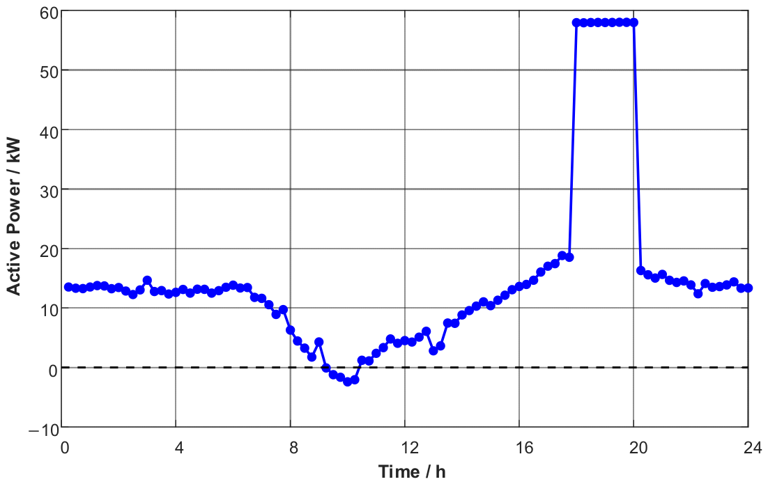
Figure 11 presents the active power transfer curve of the VSC under Scenario 2. During normal operating periods, the VSC power transfer remains relatively small and mainly provides slight power regulation according to the load and generation differences between the two transformer areas. During some daytime intervals, the VSC power transfer decreases and even approaches zero, indicating that the power support demand between the two areas is relatively weak. When the evening peak fault occurs, the active power transferred by the VSC increases rapidly and approaches its capacity limit of 58 kW. This demonstrates that, during the upstream-grid fault in Zone 1, the flexible interconnection device transfers as much available power as possible from the non-faulted area to the faulted area, thereby reducing the power supply burden on the GFM-ESS. After the fault is cleared, the VSC power transfer gradually decreases and returns to a lower level, indicating that the flexible interconnection device mainly plays a significant active support role during the fault period.

In summary, the results in Figure 10 and Figure 11 demonstrate that the proposed coordinated planning strategy can still support power exchange between different areas during the fault period on the newly introduced representative day. In addition, the voltage levels in the affected area are kept within the required security boundaries. These findings further indicate that the method has good adaptability to variations in load demand and photovoltaic output.

6. Results

This paper proposes a coordinated planning method that integrates flexible interconnections and GFM-ESSs for LVDN off-grid operation. An active support evaluation index system is embedded in the planning framework, and the nonconvex model is solved using SOCP after relaxation. Simulation results from the case analyses confirm the effectiveness of the developed framework. The key findings can be summarized as follows.

Main Findings: The coordinated configuration leverages the energy storage and network-forming capabilities of GFM-ESSs to fully compensate for the active support shortcomings of relying solely on flexible interconnection devices, thereby achieving an optimal support effect. Furthermore, quantitative analysis reveals that under constant VSC and GFM-ESS capacities, when the GFM-ESS provides a stronger power support effect to the lost load than the VSC, the placement of the GFM-ESS has a significantly greater influence on the active support performance. Specifically, placing the GFM-ESS at an intermediate node yields the optimal active support results.

Research Contributions: This study contributes a rigorous and systematic methodology by embedding newly proposed active support capability evaluation indices directly into a bi-level coordination planning model. By effectively utilizing the SOCP method to solve the complex nonconvex model, this research shifts the traditional focus from medium-voltage restoration to a low-voltage perspective, providing a reliable mathematical framework to evaluate the spatial and capacity impacts of distributed equipment on LVDN islanding operations.

Practical Value: The proposed method demonstrates profound practical advantages in both economic efficiency and power quality management. Economically, it utilizes the spatial power transfer ability of low-cost flexible interconnections to reduce the required capacity allocation of expensive GFM-ESSs, which can lower the annual comprehensive cost by approximately 18% while maintaining optimal support. Additionally, this coordinated scheme effectively mitigates the severe voltage limit violations caused by the improper connection of single-device schemes, significantly improving power quality and guaranteeing a highly reliable power supply during prolonged grid outages.

References

1. Hache, E.; Palle, A. Renewable energy source integration into power networks, research trends and policy implications: A bibliometric and research actors survey analysis. Energy Policy 2019, 124, 23–35. [Google Scholar] [CrossRef] [Scilit]
2. Kotsonias, A.; Hadjidemetriou, L.; Asprou, M.; Kyriakides, E. Operational challenges and solution approaches for low voltage distribution grids—A review. Electr. Power Syst. Res. 2025, 239, 111258. [Google Scholar] [CrossRef] [Scilit]
3. Sun, W.; Wang, Y.; Hao, Y.; Alharthi, Y.Z.; Wang, Y. A resilience-oriented optimization framework for smart grid operation and recovery before, during, and after natural disasters. Appl. Energy 2025, 398, 126414. [Google Scholar] [CrossRef] [Scilit]
4. Zhang, P.; Wang, Y.; Wang, C.; Dong, X.; Che, R.; Wu, W.; Zhang, G. Resilience Restoration Strategy for Power-Communication Coupled Networks Considering Uncertainty of Renewable Energy Output under Extreme Disasters. IEEE Trans. Ind. Appl. 2025, 62, 413–424. [Google Scholar] [CrossRef] [Scilit]
5. Yang, M.; Li, J.; Li, J.; Yuan, X.; Xu, J. Reconfiguration strategy for DC distribution network fault recovery based on hybrid particle swarm optimization. Energies 2021, 14, 7145. [Google Scholar] [CrossRef] [Scilit]
6. Guo, Z.; Lai, J.; Kou, X. Intelligent distribution network active protection and fault recovery mechanism based on DRL and graph optimization. Electr. Power Syst. Res. 2026, 254, 112623. [Google Scholar] [CrossRef] [Scilit]
7. Saaklayen, M.A.; Liang, X.; Faried, S.O.; Martirano, L.; Sutherland, P.E. Soft open point-based service restoration coordinated with distributed generation in distribution networks. IEEE Trans. Ind. Appl. 2023, 60, 2554–2566. [Google Scholar] [CrossRef] [Scilit]
8. Jiang, L.; Wang, C.; Qiu, W.; Xiao, H.; Hu, W. A flexible interconnected distribution network power supply restoration method based on E-SOP. Energies 2025, 18, 954. [Google Scholar] [CrossRef] [Scilit]
9. Stecca, M.; Elizondo, L.R.; Soeiro, T.B.; Bauer, P.; Palensky, P. A Comprehensive Review of the Integration of Battery Energy Storage Systems into Distribution Networks. IEEE Open J. Ind. Electron. Soc. 2020, 1, 46–65. [Google Scholar] [CrossRef] [Scilit]
10. Grisales-Noreña, L.F.; Cortés-Caicedo, B.; Montoya, O.D.; Hernandéz, J.C.; Alcalá, G. A Battery Energy Management System to Improve the Financial, Technical, and Environmental Indicators of Colombian Urban and Rural Networks. J. Energy Storage 2023, 65, 107199. [Google Scholar] [CrossRef] [Scilit]
11. Zhang, Y.; Yuan, C.; Du, X.; Chen, T.; Hu, Q.; Wang, Z.; Lu, J. Capacity Configuration of Hybrid Energy Storage System for Ocean Renewables. J. Energy Storage 2025, 116, 116090. [Google Scholar] [CrossRef] [Scilit]
12. Cui, Y.; Yang, G.; Yue, Y.; Zhang, Y.; Zhao, T.; Chang, X. Distributed Photovoltaic Supportability Consumption Method Considering Energy Storage Configuration Mode and Random Events. Front. Energy Res. 2024, 12, 1415175. [Google Scholar] [CrossRef] [Scilit]
13. Mallikarjun, P.; Thulasiraman, S.R.G.; Balachandran, P.K.; Zainuri, M.A.A.M. Economic Energy Optimization in Microgrid with PV/Wind/Battery Integrated Wireless Electric Vehicle Battery Charging System Using Improved Harris Hawk Optimization. Sci. Rep. 2025, 15, 10028. [Google Scholar] [CrossRef] [Scilit]
14. Yan, Z.; Li, L.; Wu, W.; Song, H.; Che, B.; Jin, P. Energy Storage Configuration and Scheduling Strategy for Microgrid with Consideration of Grid-Forming Capability. Electr. Eng. 2025, 107, 7709–7724. [Google Scholar] [CrossRef] [Scilit]
15. Hao, M.; Lan, J.; Wang, L.; Lin, Y.; Wang, J.; Qin, L. Optimized Dual-Layer Distributed Energy Storage Configuration for Voltage Over-Limit Zoning Governance in Distribution Networks. Energies 2024, 17, 1847. [Google Scholar] [CrossRef] [Scilit]
16. Tapia-Aguilera, J.; Grisales-Noreña, L.F.; Quintal-Palomo, R.E.; Montoya, O.D.; Sanin-Villa, D. Optimizing Energy Storage Systems with PSO: Improving Economics and Operations of PMGD—A Chilean Case Study. Appl. Syst. Innov. 2026, 9, 22. [Google Scholar] [CrossRef] [Scilit]
17. Cheng, X.; Wu, T.; Yao, W.; Yang, Y. Selection Method for New Energy Output Guaranteed Rates Considering Optimal Energy Storage Configuration. CSEE J. Power Energy Syst. 2024, 10, 539–547. [Google Scholar]
18. Zhong, J.; Cai, Y.; Wang, K.; Chen, Y.; Wei, X.; Su, H.; Zheng, X.; Liang, K. Two-Stage Hybrid Energy Storage Configuration Method for Distribution Networks Based on ICEEMDAN and Multi-Objective Optimization. J. Energy Storage 2025, 127, 116782. [Google Scholar] [CrossRef] [Scilit]
19. Zhou, Z.; Wen, Y.; Xia, Y.; Liu, X.; Huang, Y.; Tan, J.; Zeng, J. Fast Network Reconfiguration Method with SOP Considering Random Output of Distributed Generation. Processes 2025, 13, 3104. [Google Scholar] [CrossRef] [Scilit]
20. Kang, Y.; Lu, G.; Chen, M.; Li, X.; Li, S. Fault recovery method of DC distribution network considering EV charging and discharging and SOP network reconfiguration. Electr. Power Syst. Res. 2025, 245, 111607. [Google Scholar] [CrossRef] [Scilit]
21. Deng, M.; Liu, Y.; Hong, Y.; Sun, Z.; Hao, J. Study on the grid supporting effects for GFM energy storage system in distribution networks under grid faults. Energy Rep. 2024, 12, 5801–5813. [Google Scholar] [CrossRef] [Scilit]
22. Zhang, Y.; Xie, Y.; Cai, S.; Wu, Q.; Zhu, H.; Xiang, Z. Coordinated control of grid-forming wind turbines and grid-forming energy storage systems for power system restoration. IEEE Trans. Sustain. Energy 2025, 16, 2812–2827. [Google Scholar] [CrossRef] [Scilit]
23. Ross, B.A.; Lyu, X.; Nwaneto, U.C.; Mohiuddin, S.M.; Nassif, A.B. Using Grid-Forming Energy Storage Systems to Provide Dynamic Active Power Support for Hyperscale Data Center. IEEE Access 2026, 14, 29250–29259. [Google Scholar] [CrossRef] [Scilit]
24. Jia, Y.; Li, Q.; Liao, X.; Liu, L.; Wu, J. Research on the Access Planning of SOP and ESS in Distribution Network Based on SOCP-SSGA. Processes 2023, 11, 1844. [Google Scholar] [CrossRef] [Scilit]
25. Wang, J.; Fan, X.; Xu, L.; Shi, R.; Wang, W. Coordinated allocation of distributed generation, soft open points and energy storage systems in unbalanced distribution networks considering flexibility deficiency risk. Alex. Eng. J. 2025, 112, 569–584. [Google Scholar] [CrossRef] [Scilit]
Figure 1. LVDN flexible interconnection and GFM-ESS coordination planning model considering off-grid operation.
Energies 19 02555 g001
Figure 2. Principle diagram of feasible region convexification.
Energies 19 02555 g002
Figure 3. Grid structure.
Energies 19 02555 g003
Figure 4. Results of planning and site selection.
Energies 19 02555 g004
Figure 5. Power curve of VSC2.
Energies 19 02555 g005
Figure 6. Variation curves of comprehensive active support evaluation value with VSC capacity.
Energies 19 02555 g006
Figure 7. ENS and station area 1 line loss value.
Energies 19 02555 g007
Figure 8. A lattice structure with flexible interconnection and GFM-ESS.
Energies 19 02555 g008
Figure 9. Node voltage profiles in station area 1.
Energies 19 02555 g009
Figure 10. Voltage curves of all nodes in station area 1 under Scenario 2.
Energies 19 02555 g010
Figure 11. Active power transfer curve of the VSC under Scenario 2.
Energies 19 02555 g011