A Hierarchical Graph Neural Network with Cross-Layer Attention for Weak-Node Identification in Complex Interconnected Power Grids

Abstract

Accurate identification of weak nodes is a prerequisite for online security assessment, preventive control, and resilience enhancement in modern power systems. However, conventional single-layer graph-learning models mainly emphasize local neighborhood aggregation and are insufficient for characterizing vulnerability propagation from equipment-level disturbance to regional congestion and system-level transfer constraints. This paper proposes a mechanism-aware hierarchical graph-learning framework for weak-node identification in complex interconnected power grids. We emphasize that attention, fusion, and gating operations are standard neural-network mechanisms and are not claimed as new generic deep-learning blocks. The contribution of this paper is the power-system-specific formulation: constructing an electrically meaningful local-supernode hierarchy, defining reproducible mechanism-based node and branch-vulnerability proxies, and interpreting weak-node rankings through node–line–corridor coupling evidence. In the validated implementation, a local graph convolutional encoder and a supernode/global graph convolutional encoder generate 32-dimensional local embeddings and 16-dimensional global embeddings, which are concatenated and decoded by a 48 → 24 → 1 multilayer perceptron to obtain node vulnerability scores. Experiments are conducted on reproducible IEEE benchmark data generated from pandapower standard systems, with representative comparisons on the IEEE 57-bus, 145-bus, and 300-bus systems and a detailed structural interpretation on the IEEE 145-bus case. The present results validate the ability of the implemented local–global hierarchical model to reproduce the proposed mechanism-based vulnerability proxy on representative small- and medium-scale benchmarks.

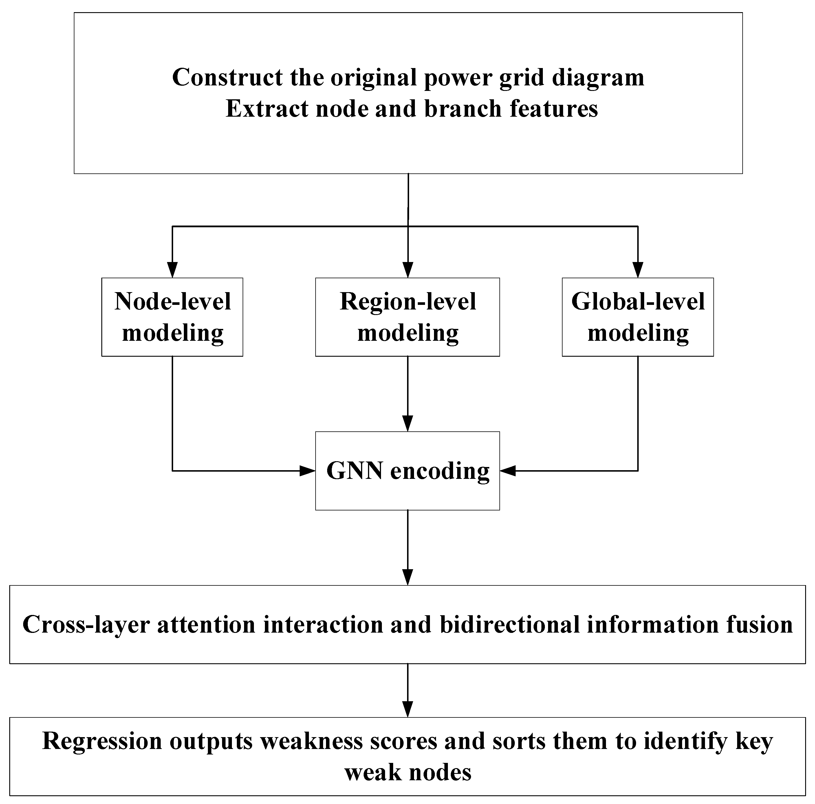
1. Introduction

1.1. Motivation

Power systems are evolving from relatively localized infrastructures into highly interconnected cyber–physical networks characterized by long-distance power transfers, multiple voltage levels, intensive inter-area exchanges, and frequent operating-point fluctuations. Under such conditions, a local disturbance seldom remains local. It can first alter the electrical environment of nearby devices, then accumulate as regional congestion or voltage stress, and finally propagate to the system level through critical transmission corridors and backbone substations. Weak-node identification should therefore be treated as a multi-scale vulnerability inference problem rather than as a purely local ranking task.

Weak-node identification has direct engineering relevance in preventive control, contingency screening, restoration planning, and online dispatch support. Nodes with high vulnerability scores are often associated with strong coupling to overloaded corridors, high voltage sensitivity, prominent responsibility in post-contingency redistribution, or persistent exposure to inter-area stress transmission. In practical dispatch environments, such nodes deserve prioritized monitoring and tighter security margins. However, many of them are not obvious from local observations alone, because an apparently moderate node may still be globally critical if it is embedded in a stressed region or connected to a transfer bottleneck.

1.2. Related Work

Early studies established the power-system vulnerability problem at the system level. Fouad et al. [1,2] formalized vulnerability as a dynamic-security concept, but their formulation did not provide a node-oriented ranking mechanism. Zhou et al. [3] introduced artificial neural networks into security and vulnerability assessment, yet the model still operated on global operating states rather than explicit network structure. Driven by the rapid development of new energy sources, inter-regional direct current transmission, and the scaled deployment of pumped-storage capabilities, the future regional power-flow exchange form will be more complex [4]. Mahadev and Christie [5,6] represented vulnerability and severity for static security assessment, but the framework remained centralized and indicator-driven.

Subsequent work enriched the physical interpretation of vulnerability. Yu and Singh [7] incorporated protection failures into integrated vulnerability analysis, but the method was still scenario-enumerative and difficult to translate into fast online weak-node scoring. Doorman et al. [8] analyzed the vulnerability of the Nordic power system using a realistic large-scale grid, but the outcome remained system-oriented rather than bus-oriented. Kamwa et al. [9,10] introduced fuzzy partitioning for dynamic vulnerability assessment, but the partition served assessment convenience rather than hierarchical representation learning. Wang et al. [11] developed a fault-chain-based vulnerability assessment scheme for transmission networks, yet the method did not learn node embeddings from graph-structured data. Chen and Mili [12] evaluated composite vulnerability to cascading failures probabilistically, but the resulting framework was not designed for dispatch-oriented weak-node ranking.

Complex-network studies further clarified an important limitation. Hines et al. [13] showed that topological models alone may provide misleading information about electricity-infrastructure vulnerability when operating conditions are ignored. Pagani and Aiello [14] reviewed the power grid as a complex network, but the dominant methodology was still based on handcrafted structural indicators rather than learnable multi-scale representations.

Neural-network-based security assessment also progressed substantially before graph learning became popular. Amjady and Ehsan [15,16] evaluated power-system reliability using artificial neural networks, but the model did not explicitly encode electrical connectivity. Amjady [17] employed time-series and fuzzy neural networks for generation-adequacy assessment, yet the formulation still focused on system-level adequacy rather than node-level vulnerability localization. Bento [18] proposed a physics-guided neural network for load-margin assessment, but the target remained operating-security margin estimation instead of weak-node identification.

The rise of graph learning created a more suitable technical basis for power-grid modeling. Wu et al. [19] reviewed graph neural networks and clarified why local message passing is effective for structured data, but the review was not power-system-specific. Zhao et al. [20] used structure-informed graph learning for online prediction of transient dynamics, but the task addressed system response forecasting rather than weak-node ranking. Gao et al. [21] proposed a physics-guided graph convolutional neural network for optimal power flow, but the goal was an OPF surrogate instead of vulnerability inference. Xie et al. [22,23] studied grid vulnerability under extreme weather and forced oscillations in the Energies literature, respectively, but these studies did not establish a hierarchical weak-node learning mechanism. Moshtagh et al. [24] developed a topology-aware graph neural network for state estimation in PMU-unobservable systems, but the task remained state reconstruction. Guo et al. [25] applied graph neural networks to production-cost minimization decomposition, but the framework targeted optimization acceleration rather than critical-node discovery. Wang et al. [26] used knowledge graphs and graph neural networks for topology identification, but the objective was network-structure recovery rather than vulnerability ranking. Kfouri et al. [27] employed graph neural networks for bad-data detection and identification in state estimation, but the emphasis was on data integrity rather than multi-scale weak-node assessment.

To make the literature positioning more focused, we now distinguish four groups of directly related methods. Classical centrality- and sensitivity-based methods provide transparent vulnerability indicators, but their scores are usually handcrafted and may not represent nonlinear regional accumulation. Physics-informed GNNs embed power-flow or operational constraints into graph learning, but most reported applications focus on OPF, state estimation, or transient-response prediction rather than dispatch-oriented weak-node ranking. Graph-transformer and attention-based methods can enlarge the receptive field, but they usually require substantial data and do not by themselves define power-grid-specific hierarchical labels. Graph-partition GNNs improve computational scalability, but graph cutting may weaken boundary and corridor information unless the partition hierarchy remains electrically coupled to the original network.

We also clarify the novelty boundary. The proposed method does not claim that GCN, attention, gating, or hierarchical pooling are new neural-network primitives. Existing GNN, GAT, GraphSAGE, GIN, ChebNet, graph-transformer, and hierarchical pooling models already provide powerful generic graph-learning operators. The scientific question addressed here is narrower and power-system-specific: how to define a weak-node target, an electrical hierarchy, and an interpretation route that connect bus-level rankings with branch vulnerability and corridor stress. Accordingly, this paper evaluates a mechanism-aware weak-node formulation rather than presenting a new universal GNN architecture.

These observations motivate a hierarchical formulation. Weak-node significance in an interconnected grid is rarely determined by one graph scale alone. Local evidence must be interpreted together with regional aggregation effects and backbone transfer constraints. A dispatch-oriented model should therefore evaluate each node through coupled local, regional, and global contexts instead of relying on a single flat graph or on disconnected partitions.

1.3. Manuscript Positioning and Main Contribution

The above literature reveals three unresolved issues directly related to weak-node identification. First, classical vulnerability studies and centrality or sensitivity indices are physically meaningful, but they mostly provide system-level indices, scenario-based assessments, or handcrafted rankings rather than learnable node-level representations. Second, modern graph-learning models such as GAT, GraphSAGE, GIN, ChebNet, graph transformers, and hierarchical pooling architectures provide generic message-passing or attention operators, but they do not by themselves define power-system weak-node labels or explain how bus vulnerability is coupled with branch and corridor stress. Third, physics-informed GNN studies in power systems mainly address OPF approximation, state estimation, topology identification, or dynamic-response prediction, whereas weak-node identification requires a target that is explicitly tied to structural, electrical, and operating-state vulnerability evidence. These gaps motivate a mechanism-aware formulation rather than a claim of inventing a new generic graph neural block.

Against this background, this paper is positioned as a mechanism-driven hierarchical extension of graph learning for weak-node identification. The fundamental difference from classical hierarchical GNNs is that the hierarchy is tied to electrical constraints: node-layer edges use admittance-type coupling, regional and backbone abstractions are induced by electrical interconnections and transfer corridors, and node scores are interpreted through branch-vulnerability and corridor-stress evidence. Thus, hierarchy is used to preserve the physical path of vulnerability propagation, namely local disturbance, regional accumulation, backbone transfer stress, and feedback to node criticality, instead of serving only as graph coarsening or computational compression.

The main contributions of this work are summarized as follows.

• A mechanism-aware weak-node formulation is proposed for complex interconnected power grids. The model uses standard graph-learning operators, but the hierarchy is defined according to electrical coupling, supernode aggregation, branch vulnerability, and corridor-level risk evidence rather than generic graph pooling alone.
• A validated local–global fusion implementation is provided. The reported numerical results are produced by a local encoder, a supernode/global encoder, assignment-based global feedback, and a 48 → 24 → 1 decoder. Attention, top-down gating, and more complex cross-scale weighting are now described only as extensible variants unless explicitly implemented.
• A reproducible vulnerability-proxy learning protocol is introduced. The reported training objective is mean-square regression on the defined mechanism-based labels, while hierarchical-consistency and ranking-loss terms are treated as future extensions and are not used as evidence for the present results.
• Based on the supplementary data-and-code package, the proposed method is validated on representative IEEE benchmark systems and analyzed in depth on the IEEE 145-bus case. The results show clear advantages in the medium-scale interconnected benchmark where inter-area coupling is particularly important, while the large-scale case is reported as a limitation rather than as universal generalization evidence.

1.4. Paper Organization

The remainder of this paper is organized as follows. Section 2 formulates the weak-node identification problem and presents the mechanism-driven hierarchical graph-construction strategy. Section 3 introduces the hierarchical representation-learning framework on the node, regional, and backbone layers. Section 4 presents the validated local–global fusion model and extensible learning strategy. Section 5 reports the benchmark configuration, comparative case studies, and engineering analysis. Section 6 concludes the paper.

2. Problem Formulation and Mechanism-Driven Hierarchical Graph Construction

2.1. Weak-Node Identification as a Multi-Criteria Vulnerability Ranking Task

Consider a power grid under operating scenario $\xi$. Let the system contain a set of buses, lines, transformers, and regional aggregation units. The task of weak-node identification is to assign each node $i$ a vulnerability score ${\widehat{N}}_i^{\xi }$ and then rank all nodes according to the predicted scores. The ranking should reflect the likelihood that a node acts as a structurally and operationally critical weak point under the given scenario.

Different from generic node classification, vulnerability ranking in a power grid is driven by both structural role and operating-state sensitivity. A desirable predictor should satisfy at least four requirements:

• It should detect local stress, such as voltage deviation, loading imbalance, or weak neighborhood support.
• It should capture regional aggregation effects, such as area-level congestion or concentrated stress in a station cluster.
• It should reflect global transfer constraints, especially the influence of critical corridors and backbone interconnections.
• It should preserve the ordering of high-risk nodes, rather than merely fitting their numerical scores in a mean-square sense.

These requirements imply that the desired predictor is inherently multi-scale.

2.2. Limitations of Single-Layer Graph Representations for Weak-Node Assessment

A single-layer graph representation models the grid as a graph $G=(V,E)$, where all buses or substations appear at the same level. This representation is useful for local message passing but insufficient for two reasons.

First, the physical consequence of a disturbance is not confined to the immediate neighbors of the disturbed equipment. Post-contingency power redistribution may raise stress in one region, then shift transfer pressure into an adjacent corridor, and finally create a vulnerability cluster around a different set of nodes. Second, nodes with similar local neighborhoods may play substantially different roles when embedded in different higher-level structures. Therefore, two nodes that are locally similar can still exhibit markedly different global vulnerability.

2.3. Hierarchical Risk Propagation in Interconnected Power Grids

The supplementary data-and-code package and the accompanying case-study files indicate that vulnerability propagation in interconnected grids follows a hierarchical path rather than a simple additive aggregation. This path can be expressed as

“local equipment disturbance” → ”regional accumulation” → ”backbone transfer stress” → ”feedback to node vulnerability”.

This interpretation provides the conceptual basis for the hierarchical model proposed in this paper. The node layer captures immediate electrical interactions around equipment. The regional layer captures station-cluster or partition-level stress accumulation. The backbone/global layer captures long-range transfer coupling and corridor constraints. Weak-node identification then becomes the problem of adaptively fusing these three levels.

2.4. Scenario-Aware Construction of the Node-Layer Graph

For a given scenario ξ, the node layer is defined as

$$G_{\xi }^0=(V^0,E^0,A_{\xi }^0,X_{\xi }^0)$$

(1)

where $V^0$ is the node set, $E^0$ is the branch/transformer connection set, $A_{\xi }^0$ is the scenario-dependent weighted adjacency matrix, and $X_{\xi }^0$ is the node-feature matrix. $G_{\xi }^0$ represents the node-layer power-grid diagram constructed under scenario ξ, used to describe the basic network structure and node connection relationships under this operating scenario.

The scenario-dependent edge weight is modeled as

$$A_{ij,\xi }^0=u_{ij}^{\xi }{w}_{ij}$$

(2)

where $u_{ij}^{\xi }\in \left[\mathrm{0,1}\right]$ is the availability coefficient of branch $i-j$ under scenario $\xi$, and $w_{ij}$ is the basic electrical coupling coefficient. $A_{ij,\xi }^0$ represents the node-level weighted adjacency coefficient between node $i$ and node $j$ in scenario $\xi$, used to characterize the effective electrical coupling strength between them.

In the general formulation, $u_{ij}^{\xi }$ can be determined from switch status, protection action, maintenance outage, or post-contingency line-state assessment, while $w_{ij}$ can be computed from line impedance, transformer equivalent parameters, or admittance-based coupling. In the released implementation used for the benchmark study, the node-layer graph is instantiated with admittance-type edge weights derived from ‘pandapower’ network data, and in-service transformers are retained as strong interconnection links.

This formulation prevents the graph from degenerating into a purely topological object. Instead, the graph becomes a scenario carrier that reflects the effective propagation capability of electrical interactions.

2.5. Node-Feature Representation and Physical Interpretability

The general mechanism-aware formulation allows static topology features, operating-state features, and disturbance-response features to be combined. The current benchmark implementation in the supplementary data-and-code package adopts a six-dimensional feature vector that is traceable to the training scripts. For each node, the feature vector contains

• Node degree;
• Weighted betweenness centrality;
• Sampled weighted average shortest-path length;
• Weighted clustering coefficient;
• Voltage-deviation magnitude;
• Normalized active load.

Accordingly, the node-feature vector for node i under scenario ξ is written as

$${\mathit{x}}_i^{0,\xi }=[d_i,c_i^{\mathrm{bet}},{\mathcal{l}}_i^{\mathrm{avg}},c_i^{\mathrm{clus}},\mathsf{\Delta }{v}_i,p_i^{\mathrm{norm}}]$$

(3)

where ${\mathit{x}}_i^{0,\xi }$ denotes the input feature vector of node $i$ in the node layer under scenario $\xi$, $d_i$ denotes the degree of node $i$, reflecting its direct topological connectivity, $c_i^{\mathrm{bet}}$ denotes the weighted betweenness centrality of node $i$, measuring its importance on weighted shortest paths, ${\mathcal{l}}_i^{\mathrm{avg}}$ denotes the sampled weighted average shortest-path length from node $i$ to the other nodes, $c_i^{\mathrm{clus}}$ denotes the weighted clustering coefficient of node $i$, characterizing the local connectivity density around the node, $\mathsf{\Delta }{v}_i$ denotes the voltage-deviation magnitude of node $i$, indicating its operating-state stress, and $p_i^{\mathrm{norm}}$ denotes the normalized active load of node $i$.

The first four components describe the structural role of the node in the electrical interaction graph, while the last two components reflect operating-state stress. This compact feature set preserves physical interpretability.

2.6. Node-to-Region Assignment and Regional Abstraction

To lift local information to the regional scale, a node-to-region assignment matrix is introduced:

$$S^0\in \{\mathrm{0,1}{\}}^{N\times M}$$

(4)

where $N$ is the number of nodes and $M$ is the number of regional units. $S^0$ is the node-to-region assignment matrix that maps node-layer nodes to regional units.

Each row of $S^0$ indicates the region to which a node belongs. Depending on the engineering setting, the region can correspond to a station cluster, a voltage-level group, or a dispatch partition. Region-like supernodes are obtained by spectral clustering or size-constrained grouping, which yields an adaptive partition consistent with system scale.

2.7. Regional Feature Aggregation and Inter-Region Coupling

The regional feature matrix is obtained by average aggregation:

$$H^1={\displaystyle \frac{{\left(S^0\right)}^{\top }{H}^0}{{\left(S^0\right)}^{\top }\mathbf{1}}}$$

(5)

where $H^0$ denotes the node-level hidden feature matrix and $\mathbf{1}$ is an all-one vector. $H^1$ denotes the regional feature matrix obtained by aggregating node-level representations within each region.

The regional adjacency matrix is generated by lifting node-layer interactions:

$$A^1={\left(S^0\right)}^{\mathrm{\top }}{A}^0{S}^0$$

(6)

where $A^1$ denotes the regional adjacency matrix induced from node-layer interactions, and $A^0$ denotes the node-layer adjacency matrix before regional lifting.

This formulation retains inter-region coupling without requiring handcrafted region-level edges. A dense set of cross-region electrical links in the node graph automatically induces strong edges in the regional graph.

2.8. Region-to-Backbone Aggregation and Global Representation

A second assignment matrix is used to aggregate regional units into the backbone/global layer:

$$S^1\in \{\mathrm{0,1}{\}}^{M\times K}$$

(7)

where $K$ is the number of backbone units, and $S^1$ denotes the region-to-backbone assignment matrix that maps regional units to the backbone/global layer.

The corresponding global features and adjacency are

$$\begin{array}{c}{H}^2=\frac{{\left(S^1\right)}^{\mathrm{T}}{H}^1}{{\left(S^1\right)}^{\mathrm{T}}\mathbf{1}},\\ A^2={\left(S^1\right)}^{\mathrm{T}}{A}^1{S}^1\end{array}$$

(8)

where $H^2$ denotes the backbone/global feature matrix obtained by aggregating regional representations. $A^2$ denotes the backbone/global adjacency matrix induced from inter-region couplings.

The backbone/global layer abstracts higher-level transfer channels and system-wide constraints. From a power-system perspective, this layer is essential because long-range vulnerability is usually governed by backbone corridors rather than by individual branches alone.

2.9. Mechanism-Driven Vulnerability Labels

For the paper formulation, the node target is interpreted as a multi-scale vulnerability quantity synthesized from local, regional, and global components:

$$N_i={\kappa }_1{N}_i^{\mathrm{local}}+{\kappa }_2{N}_i^{\mathrm{regional}}+{\kappa }_3{N}_i^{\mathrm{global}}$$

(9)

where ${\kappa }_1,{\kappa }_2,{\kappa }_3$ are adaptive contribution coefficients, $N_i$ denotes the overall vulnerability score of node $i$, $N_i^{\mathrm{local}}$ denotes the local vulnerability component of node $i$, reflecting risks caused by its immediate neighborhood, $N_i^{\mathrm{regional}}$ denotes the regional vulnerability component of node $i$, reflecting risks inherited from its regional cluster, and $N_i^{\mathrm{global}}$ denotes the global vulnerability component of node $i$, reflecting risks associated with system-wide backbone conditions.

This decomposition is important because the learning target is not treated as an arbitrary label; it is treated as a reproducible mechanism-based proxy for dispatch-oriented weak-node ranking.

The practical label-generation procedure used for the benchmark data is summarized as follows. Step 1: a standard pandapower benchmark case is loaded and converted into an admittance-weighted graph in which in-service transmission lines and transformers define the effective electrical coupling. Step 2: node-level structural and operating indicators are computed, including degree, weighted betweenness centrality, sampled weighted average shortest-path length, weighted clustering coefficient, voltage-deviation magnitude, and normalized active load. Step 3: branch-vulnerability indicators are computed from normalized electrical-coupling and path/corridor-related quantities, and the branch-vulnerability score is stored as the branch target. Step 4: node vulnerability evidence is aggregated from its own structural-operating indicators, the vulnerability of incident or nearby branches, and the regional/corridor context induced by the graph hierarchy. Step 5: each component is min–max normalized within the case to avoid scale dominance, and the final reference node score is obtained by averaging or weighted synthesis of the normalized components.

Therefore, the reference ranking is a mechanism-based weak-node index derived from topology, electrical coupling, bus operating stress, and branch–corridor vulnerability evidence. It is not a label manually assigned by experts. It is also not a complete dynamic cascading-failure label; rather, it is a transparent and reproducible proxy designed for supervised weak-node ranking when full N − 1 or dynamic cascading simulations are not available for all benchmark systems.

For clarity, the current branch-vulnerability proxy is defined from normalized electrical-coupling and corridor-stress indicators, including path/corridor importance, line coupling strength, and loading- or stress-related quantities available from the processed benchmark data. The current node vulnerability proxy combines four categories of normalized evidence: local structural/electrical support, bus operating stress, incident or neighboring branch vulnerability, and regional/global aggregation induced by the hierarchy. These normalized components are synthesized to obtain the final node score used for supervised learning.

3. Hierarchical Multi-Level Representation Learning

3.1. Overall Framework of the Proposed Hierarchical GNN

Figure 1 illustrates the overall workflow of the proposed method. Starting from the original power-grid diagram, the method first extracts node and branch features and constructs the graph representation of the system. The resulting information is processed through coordinated local and supernode/global modeling levels so that local electrical characteristics, regional aggregation effects, and system-wide transfer constraints can be represented simultaneously. The validated implementation uses local and global GCN encoders followed by embedding fusion and regression decoding, while the generalized framework also permits attention-based interaction when sufficient data are available. Finally, the regression module outputs weakness scores for all candidate nodes and ranks them to identify the key weak nodes in the interconnected power grid.

Figure 1 illustrates the overall workflow of the proposed hierarchical graph neural network for weak-node identification. Starting from the original power-grid diagram, the method first extracts node and branch features and constructs the graph representation of the system. The resulting information is then processed through three coordinated modeling levels, namely node-level modeling, region-level modeling, and global-level modeling, so that local electrical characteristics, regional aggregation effects, and system-wide transfer constraints can be represented simultaneously. After GNN encoding is performed on each level, cross-layer attention interaction and bidirectional information fusion are introduced to exchange information across scales and refine node representations. Finally, the regression module outputs weakness scores for all candidate nodes and ranks them to identify the key weak nodes in the interconnected power grid.

3.2. Node-Level Representation Learning

After graph construction, local message passing is performed on the node layer. Let $H_{\mathrm{loc}}^l$ denote the hidden representation at layer $l$, and let ${\tilde{A}}^0$ denote the normalized node-layer adjacency matrix. The local encoder is formulated as

$$H_{\mathrm{loc}}^{l+1}=\sigma \left({\tilde{A}}^0{H}_{\mathrm{loc}}^l{W}_{\mathrm{loc}}^l\right)$$

(10)

where $W_{\mathrm{loc}}^l$ is a learnable weight matrix and $\sigma (·)$ is a nonlinear activation function, and $H_{\mathrm{loc}}^l$ denotes the local hidden representation after the $l$-th graph-convolution layer. $H_{\mathrm{loc}}^{l+1}$ denotes the local hidden representation after the $(l+1)$-th graph-convolution layer.

The local encoder uses two graph-convolution layers. One implementation adopts a $6\to 64\to 32$ structure, which produces 32-dimensional local node embeddings. This stage is responsible for capturing short-range interactions such as local congestion, neighboring voltage stress, and immediate structural support.

3.3. Regional and Backbone Representation Learning

Regional encoding is performed on the lifted regional graph:

$$H_{\mathrm{reg}}^{l+1}=\sigma \left({\tilde{A}}^1{H}_{\mathrm{reg}}^l{W}_{\mathrm{reg}}^l\right)$$

(11)

where ${\tilde{A}}^1$ is the normalized regional adjacency matrix, $H_{\mathrm{reg}}^{l+1}$ denotes the regional hidden representation after the $(l+1)$-th regional graph-convolution layer, $H_{\mathrm{reg}}^l$ denotes the regional hidden representation at layer $l$, and $W_{\mathrm{reg}}^l$ denotes the learnable weight matrix used in the regional encoder at layer $l$.

The regional encoder allows region-level semantics to be learned directly from the aggregated graph rather than being inferred indirectly from node embeddings only.

The backbone/global layer is encoded as

$$H_{\mathrm{glo}}^{l+1}=\sigma \left({\tilde{A}}^2{H}_{\mathrm{glo}}^l{W}_{\mathrm{glo}}^l\right)$$

(12)

where $H_{\mathrm{glo}}^{l+1}$ denotes the global hidden representation after the $(l+1)$-th backbone/global graph-convolution layer, ${\tilde{A}}^2$ denotes the normalized adjacency matrix of the backbone/global layer, $H_{\mathrm{glo}}^l$ denotes the global hidden representation at layer $l$, and $W_{\mathrm{glo}}^l$ denotes the learnable weight matrix used in the backbone/global encoder at layer $l$.

This layer captures system-wide transfer dependencies and long-range structural constraints. In the implemented comparison model, the supernode/global encoder outputs 16-dimensional features, which are transmitted back to nodes according to the cluster assignment.

4. Validated Local–Global Fusion Model and Extensible Learning Strategy

4.1. Cross-Layer Attention for Inter-Scale Dependency Modeling

The central innovation of the model is that inter-layer influence is not handled by fixed averaging. Instead, a node learns which higher-layer unit matters most to it through cross-layer attention.

For a lower-layer node $i$ in layer $l$ and an upper-layer unit $j$ in layer $m$, the unnormalized cross-layer attention score is

$$e_{l\to m}{\displaystyle (i,j)}={\displaystyle \frac{{\left(W_q{h}_i^l\right)}^{\top }\left(W_k{h}_j^m\right)}{\sqrt{d}}}$$

(13)

where $W_q$ and $W_k$ are learnable query and key transforms, respectively, and $d$ is the attention dimension, $e_{l\to m}(i,j)$ denotes the unnormalized cross-layer attention score from lower-layer unit $i$ in layer $l$ to upper-layer unit $j$ in layer $m$, $h_i^l$ denotes the hidden embedding of unit $i$ in layer $l$, and $h_j^m$ denotes the hidden embedding of unit $j$ in layer $m$.

The normalized attention coefficient is then

$$a_{l\to m}{\displaystyle (i,j)}={softmax}_j\left(e_{l\to m}(i,j)\right)$$

(14)

where $a_{l\to m}(i,j)$ denotes the normalized cross-layer attention coefficient measuring the contribution of upper-layer unit $j$ to lower-layer unit $i$, and ${\mathrm{s}\mathrm{o}\mathrm{f}\mathrm{t}\mathrm{m}\mathrm{a}\mathrm{x}}_j(·)$ denotes the softmax operation performed over all candidate upper-layer units indexed by $j$.

This formulation gives the model a clear physical interpretation: a node may be affected more strongly by some regional or backbone units than by others, even when these units belong to the same upper-level graph. Hence, the model is not a simple additive hierarchy, it is an adaptive inter-scale influence hierarchy.

4.2. Bottom-Up Semantic Aggregation and Top-Down Contextual Feedback

Bottom-up aggregation transfers higher-level semantics to the node representation. A generic formulation is

$$h_i^{\uparrow }={\sum }_j{a}_{0\to 1}{\displaystyle (i,j)}{W}_v^{\left(1\right)}{h}_j^1+{\sum }_k{a}_{0\to 2}{\displaystyle (i,k)}{W}_v^{\left(2\right)}{h}_k^2$$

(15)

where $W_v^{\left(1\right)}$ and $W_v^{\left(2\right)}$ are value transforms for the regional and backbone layers, and $h_i^{\uparrow }$ denotes the bottom-up aggregated representation of node $i$ obtained from higher-layer semantics.

This operation means that a node receives information about its hosting region and the stress pattern of the backbone structure to which it is coupled. In engineering terms, a locally moderate node can still become a high-priority weak node if the surrounding region is congested or if the relevant transfer corridor is critically loaded.

Bottom-up transfer alone is insufficient, because the model also requires a feedback mechanism to refine local semantics using global context. The feedback term is written as

$$h_i^{\downarrow }=\varphi (h_i^0,h_i^{\uparrow })$$

(16)

where $\varphi (·)$ denotes a learnable refinement function implemented in practice through neural fusion layers, and $h_i^{\downarrow }$ denotes the top-down refined representation of node $i$ after contextual feedback from higher-level information.

This design corresponds to the physical understanding that system-wide constraints may change how local evidence should be interpreted. A moderate local stress should be scored differently depending on whether it occurs in a relaxed area or in a corridor-adjacent region already close to its transfer limit.

4.3. Adaptive Fusion and Final Vulnerability Scoring

To avoid hard-coded fusion ratios, the model introduces a gate to determine the relative contribution of bottom-up and top-down signals:

$$\begin{array}{c}{g}_i=\sigma \left(W_g\right[h_i^0;h_i^{\uparrow };h_i^{\downarrow }]+b_g)\\ h_i^{\mathrm{fuse}}=g_i\odot h_i^{\uparrow }+(1-g_i)\odot h_i^{\downarrow }\end{array}$$

(17)

where the gate $g_i$ is node-dependent, $W_g$ denotes the learnable weight matrix in the adaptive gating module, $b_g$ denotes the bias term in the adaptive gating module, $h_i^{\mathrm{fuse}}$ denotes the fused representation of node $i$ obtained by combining bottom-up and top-down information, and $\odot$ denotes element-wise multiplication.

Therefore, different nodes can be dominated by different scales of risk. This directly addresses the concern that weak-node identification should not be reduced to a fixed weighted sum.

The final vulnerability score is predicted through a multilayer perceptron operating on the concatenation of the local and fused representations:

$${\widehat{N}}_i=MLP\left(\right[h_i^0;h_i^{\mathrm{fuse}}\left]\right)$$

(18)

where ${\widehat{N}}_i$ denotes the predicted vulnerability score of node $i$, and $\mathrm{M}\mathrm{L}\mathrm{P}(\cdot )$ denotes the multilayer perceptron used to map the concatenated embeddings to the final vulnerability score.

4.4. Learning Objective with Consistency and Ranking Terms

Weak-node identification is meaningful only if the model predicts both accurate scores and correct priorities. We therefore consider a composite objective:

$$L=L_{\mathrm{reg}}+{\lambda }_1{L}_{\mathrm{cons}}+{\lambda }_2{L}_{\mathrm{rank}}$$

(19)

where $L$ denotes the total training loss, $L_{\mathrm{reg}}$ denotes the regression loss between the predicted vulnerability score and the target vulnerability score, ${\lambda }_1$ denotes the weighting coefficient for the consistency loss, $L_{\mathrm{cons}}$ denotes the hierarchical-consistency loss that penalizes inconsistency between node-level predictions and higher-level semantics, ${\lambda }_2$ denotes the weighting coefficient for the ranking loss, and $L_{\mathrm{rank}}$ denotes the pairwise ranking loss used to preserve the correct vulnerability ordering among nodes.

The regression loss is

$$L_{\mathrm{reg}}={\displaystyle \frac{1}{N}}{\sum }_{i=1}^N{({\widehat{N}}_i-N_i)}^2$$

(20)

A hierarchical-consistency term can be used to penalize contradictions between node-level predictions and higher-level semantics; e.g.,

$$L_{\mathrm{cons}}={\sum }_r{\Vert {\overline{N}}_r-\psi \left(H_r^1\right)\Vert }_2^2+{\sum }_g{\Vert {\overline{N}}_g-\phi \left(H_g^2\right)\Vert }_2^2$$

(21)

where ${\overline{N}}_r$ and ${\overline{N}}_g$ denote aggregated vulnerability estimates at the regional and backbone levels, and $\psi (·)$, $\phi (·)$ are learnable projections, $\parallel \cdot {\parallel }_2^2$ denotes the squared $L_2$-norm used to measure the discrepancy penalty.

To improve dispatch-oriented ranking stability, a pairwise ranking term can also be incorporated:

$$L_{\mathrm{rank}}={\sum }_{(i,j)\in \Omega }max\left(\mathrm{0,1}-({\widehat{N}}_i-{\widehat{N}}_j)sign(N_i-N_j)\right)$$

(22)

where $\Omega$ is a set of sampled node pairs, and $\mathrm{s}\mathrm{i}\mathrm{g}\mathrm{n}(\cdot )$ denotes the sign function that indicates whether a value is positive, negative, or zero.

4.5. Reproducibility and Implementation Boundary

The manuscript is grounded in a reproducible supplementary data-and-code package rather than in an unspecified local source. The following details can be traced directly to the released files:

• The benchmark data are loaded from ‘pandapower’ standard network cases.
• The training data directory is ‘GNN/multi_case_dataset’.
• The node features are six-dimensional and include graph topology metrics, voltage deviation, and load magnitude.
• The hierarchical trainer includes a two-stage GCN architecture, with a local encoder, a global/supernode encoder, and a node decoder.
• The comparison script evaluates three methods: original GNN, graph-partition GNN, and hierarchical GNN.
• The evaluation metrics include MSE, MAE, Spearman correlation, Hit@3, Hit@5, and Hit@10.
• The fixed random seed is 42 in the main comparison scripts and spectral clustering/K-means partitioning steps.
• The software environment used for the present revision is Python 3.11.9, PyTorch 2.11.0+cpu, torch_geometric 2.7.0, pandapower 3.4.0, NetworkX 3.6.1, NumPy 2.3.5, SciPy 1.16.3, and scikit-learn 1.8.0.

5. Case Studies and Experimental Analysis

5.1. Benchmark Systems and Data Sources

The supplementary data-and-code package contains multiple IEEE and PEGASE benchmark systems used to generate graph data. The cases explicitly listed in the hierarchical training script are summarized in

Table 1. Benchmark systems available in the supplementary data-and-code package.

Category	Systems
Small scale	case14, case24_ieee_rts, case30, case33bw, case39
Medium scale	case57, case89pegase, case118, case145, case_illinois200
Large scale	case300, case1354pegase

.

These systems provide a diverse range of topologies and scales. The IEEE 145-bus system plays a central role in this paper because the supplementary package contains node labels, branch labels, a topology figure, a detailed case report, and ranking tables for both nodes and lines.

5.2. Labels, Evaluation Metrics, and Baseline Methods

Node labels are stored as the final vulnerability target $N$, while branch labels are stored as the branch-vulnerability target $B$ and its intermediate decomposition terms. The detailed branch ranking table confirms that several of the highest-risk branches are concentrated around a compact set of nodes, which supports the coupling hypothesis that motivates the hierarchical model.

The following metrics are used throughout the comparison:

• MSE: score regression accuracy;
• MAE: absolute deviation of predicted vulnerability scores;
• Spearman coefficient: ranking consistency between predictions and mechanism-based labels;
• Hit@3, Hit@5, Hit@10: overlap ratio between predicted and reference top-$k$ weak nodes.

These metrics are complementary. MSE and MAE evaluate numerical fidelity, while Spearman and Hit@$k$ directly evaluate whether the model identifies the correct critical nodes.

Furthermore, we added a supplementary fixed-seed baseline comparison including GAT, GraphSAGE, GIN, ChebNet, TransformerConv, and two classical vulnerability proxies based on degree and betweenness. These baselines were trained or evaluated under the same processed feature-label protocol for the three representative systems. The results are reported in

Table 2. Comparison of different methods.

Case	Method	MSE	MAE	Spearman	Hit@3	Hit@5	Hit@10
case57	Original GNN	0.0359	/	0.248	67%	40%	30%
case57	Graph-partition GNN	0.0191	/	0.220	0%	0%	20%
case57	Hierarchical GNN	0.0088	/	0.591	67%	60%	70%
case57	GAT	0.0177	0.1005	0.500	67%	40%	50%
case57	GraphSAGE	0.0102	0.0795	0.641	67%	60%	80%
case57	GIN	0.0109	0.0769	0.642	67%	60%	80%
case57	ChebNet	0.0085	0.0720	0.620	100%	60%	90%
case57	TransformerConv	0.0101	0.0766	0.688	67%	60%	70%
case57	Degree index	0.0705	0.2253	0.719	67%	60%	70%
case57	Betweenness index	0.0624	0.1922	0.282	67%	40%	20%
case145	Original GNN	0.0161	/	0.680	33%	40%	40%
case145	Graph-partition GNN	0.0207	/	0.702	33%	20%	30%
case145	Hierarchical GNN	0.0068	/	0.825	67%	60%	50%
case145	GAT	0.0240	0.1274	0.685	0%	0%	0%
case145	GraphSAGE	0.0152	0.0973	0.747	0%	20%	20%
case145	GIN	0.0124	0.0828	0.827	0%	40%	50%
case145	ChebNet	0.0095	0.0719	0.768	67%	40%	40%
case145	TransformerConv	0.0125	0.0820	0.797	0%	20%	30%
case145	Degree index	0.0373	0.1425	0.773	67%	40%	30%
case145	Betweenness index	0.0459	0.1389	0.335	0%	20%	20%
case300	Original GNN	0.0266	/	0.394	0%	0%	20%
case300	Graph-partition GNN	0.0147	/	−0.125	0%	0%	0%
case300	Hierarchical GNN	0.0135	/	−0.025	0%	0%	10%
case300	GAT	0.0141	0.0934	0.354	33%	20%	20%
case300	GraphSAGE	0.0175	0.1025	0.467	33%	20%	30%
case300	GIN	0.0138	0.0898	0.472	33%	40%	40%
case300	ChebNet	0.0158	0.0886	0.504	33%	20%	10%
case300	TransformerConv	0.0178	0.1009	0.438	33%	20%	20%
case300	Degree index	0.0653	0.2055	0.472	33%	20%	10%
case300	Betweenness index	0.0480	0.1287	0.343	0%	0%	10%

. They show that modern GNN variants can be competitive, especially GIN and ChebNet on some metrics; therefore, we further narrow our claim. The present contribution is not a universal performance dominance over all graph models, but a mechanism-aware weak-node formulation and an interpretable local–global hierarchy whose strongest numerical evidence remains the IEEE 145-bus case and the node–line–corridor coupling analysis.

The expanded comparison indicates that no single model dominates all metrics and all cases. For example, ChebNet obtains a low MSE on case57 and GIN obtains a high Spearman coefficient on case145, whereas the hierarchical GNN gives the lowest MSE on case145 and remains directly tied to the proposed node–line–corridor interpretation. This result supports a more cautious conclusion: the proposed formulation is competitive and interpretable on the target medium-scale interconnected benchmark, but broader claims require further repeated-run studies, hyperparameter tuning, physics-informed baselines, and full ablation experiments.

A full expanded benchmark should include: (i) flat GCN, GAT, GraphSAGE, GIN, ChebNet, and graph-transformer models trained under the same feature and label protocol; (ii) physics-informed GNN variants with power-flow residuals or sensitivity constraints; (iii) classical degree, betweenness, electrical centrality, voltage-sensitivity, and contingency-based vulnerability indices; and (iv) ablations that remove the hierarchy, remove the supernode/global encoder, replace local–global fusion with local-only prediction, vary the region-construction strategy, and test any ranking or consistency loss separately.

• Original GNN: a two-layer graph-convolution encoder on the full graph that decodes node and branch vulnerability directly.
• Graph-partition GNN: a partition-based baseline that first divides the graph into local subgraphs and then trains local graph models independently, mainly reflecting the computational-partitioning route.
• Hierarchical GNN: the proposed method that forms supernodes from lower-layer groups, performs local and global graph convolution, and fuses the resulting representations for node scoring.

5.3. Detailed IEEE 145-Bus Case Configuration

The case study reports that the selected IEEE 145-bus benchmark has 133 effective nodes and 358 branch samples in the processed experimental dataset. This processed case therefore serves as a medium-scale representative system where local, regional, and corridor-level effects can all be observed clearly.

The IEEE 145-bus case is particularly suitable for structural interpretation because the supplementary package provides synchronized evidence at three levels: node vulnerability labels, branch-vulnerability rankings, and a topology visualization. This combination makes it possible to examine whether the predicted weak nodes coincide with corridor-dominated high-risk regions rather than being isolated local anomalies.

5.4. Computational Considerations

For a three-layer hierarchy, the approximate per-layer message-passing complexity is proportional to $\mathcal{O}\left(\left|E^0\right|d+\left|E^1\right|d+\left|E^2\right|d\right)$, where $d$ is the hidden dimension. Since $\left|E^1\right|$ and $\left|E^2\right|$ are much smaller than $\left|E^0\right|$, hierarchical encoding offers a computationally reasonable trade-off between expressive power and scalability. In practice, the local scripts either limit cluster size or set the number of supernodes adaptively according to network size, which keeps the upper-layer graphs compact.

5.5. Cross-System Comparative Results

The case study contains cross-method comparisons on three representative systems: IEEE 57-bus, IEEE 145-bus, and IEEE 300-bus. The results are listed in

Table 3. Cross-method performance comparison on representative benchmark systems.

Case	Nodes	Method	MSE	Spearman	Hit@3	Hit@5	Hit@10
case57	57	Original GNN	0.0359	0.248	67%	40%	30%
case57	57	Hierarchical GNN	0.0088	0.591	67%	60%	70%
case145	133	Original GNN	0.0161	0.680	33%	40%	40%
case145	133	Hierarchical GNN	0.0068	0.825	67%	60%	50%
case300	241	Original GNN	0.0266	0.394	0%	0%	20%
case300	241	Hierarchical GNN	0.0135	−0.025	0%	0%	10%
case57	57	Graph-Partition GNN	0.0191	0.220	0%	0%	20%
case145	133	Graph-Partition GNN	0.0207	0.702	33%	20%	30%
case300	241	Graph-Partition GNN	0.0147	−0.125	0%	0%	0%

.

Several important observations can be drawn from Table 3. First, the hierarchical model delivers the clearest advantage on the medium-scale interconnected benchmark represented by case145. Its MSE is reduced substantially from 0.0161 to 0.0068 relative to the original GNN and from 0.0207 to 0.0068 relative to the graph-partition GNN, while the Spearman coefficient reaches 0.825. This result is highly relevant for the targeted engineering scenario of this paper, because medium-scale interconnected systems are exactly the systems where local interactions and inter-area couplings are both important.

Second, the improvement on case57 indicates that explicit scale separation is beneficial even when the graph itself is not extremely large. The model significantly improves ranking quality, reaching 70% Hit@10 and 60% Hit@5, which suggests that hierarchical structure enhances ranking stability even in relatively compact systems.

Third, the case300 results indicate that the present implementation still faces challenges on larger systems with weaker structural regularity or reduced label coverage. This is an important and honest observation. It shows that hierarchical graph learning is not a universal remedy by itself; performance still depends on training coverage, label quality, and the adequacy of the region/backbone abstraction.

Overall, the representative comparisons support a moderated claim: hierarchical modeling is particularly effective when weak-node significance is governed by cross-scale propagation rather than by purely local patterns, but the present evidence should not be interpreted as proof of universal large-scale generalization.

5.6. Structural Interpretation of the IEEE 145-Bus Case

The IEEE 145-bus system is the most informative case in the supplementary package and is therefore used for detailed structural analysis.

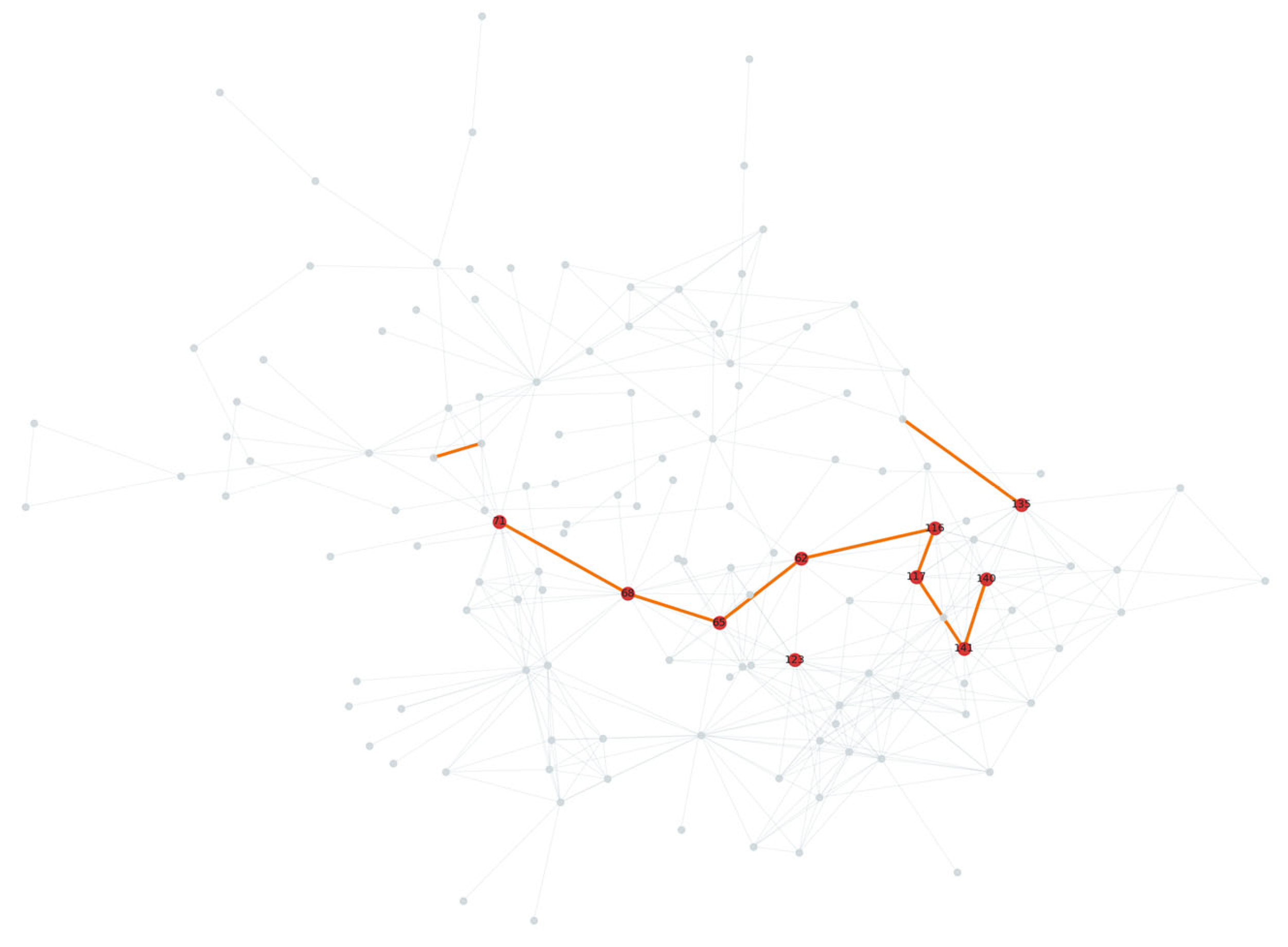
Figure 2 provides a topology-centered interpretation of the case145 benchmark. In the figure, the red nodes denote the top-10 weak buses in the mechanism-based node ranking, whereas the orange line segments denote the top-10 weak transmission lines in the branch-vulnerability ranking. The notable spatial overlap between the highlighted nodes and highlighted line segments indicates that weak nodes are not scattered randomly across the network. Instead, they concentrate around a limited number of corridor-dominated transfer paths, especially in the regions surrounding Buses 68, 71, 140, 141, 62, 65, 116, and 117. This visual evidence is important because it shows that the target of weak-node identification is physically coupled to branch-level transmission bottlenecks and regional stress accumulation.

Table 4. Top-ranked weak nodes in the IEEE 145-bus case.

Rank	Reference Weak Node	Reference Score	Hierarchical Prediction	Predicted Score
1	Bus 141	0.8408	Bus 141	0.6470
2	Bus 71	0.7661	Bus 68	0.6200
3	Bus 68	0.6713	Bus 123	0.5880
4	Bus 140	0.6002	Bus 135	0.5280
5	Bus 65	0.5385	Bus 140	0.5130
6	Bus 123	0.5385	Bus 120	0.5070
7	Bus 116	0.5384	Bus 58	0.5050
8	Bus 117	0.5350	Bus 130	0.4910
9	Bus 62	0.5229	Bus 73	0.4810
10	Bus 135	0.5095	Bus 66	0.4730

compares the top-ranked weak nodes in the reference mechanism labels and in the hierarchical prediction.

The most important observation is that the hierarchical model correctly identifies Bus 141 as the most critical weak node and retrieves several other structurally meaningful nodes, including Bus 68, Bus 123, Bus 135, and Bus 140. Compared with the original GNN, the hierarchical model exhibits a much stronger alignment with the corridor-centered high-risk structure visible in the branch ranking.

This result is not accidental. The highly ranked predicted nodes are not simply the nodes with strong local activity; they are nodes embedded in a stress-transmission structure. The success of the hierarchical model therefore supports the theoretical argument that node vulnerability depends on both local evidence and higher-layer context.

5.7. Node–Line Coupling Evidence and Representative Critical Buses

The branch ranking file provides strong support for the above interpretation. The top-10 branch vulnerabilities in the IEEE 145-bus case are listed in

Table 5. Top-ranked branch vulnerabilities in the IEEE 145-bus case.

Rank	from Bus	to Bus	Branch Vulnerability $\mathit{B}$
1	68	71	1.0000
2	140	141	0.8265
3	62	65	0.7728
4	141	142	0.7359
5	65	68	0.6957
6	62	116	0.6254
7	116	117	0.5697
8	117	142	0.5686
9	134	135	0.5007
10	97	99	0.4943

.

The coupling between the node ranking and the branch ranking is striking. The reference weak nodes 141, 68, 140, 65, 123, 116, 117, 62, and 135 are tightly distributed around the high-risk branches 68–71, 140–141, 62–65, 141–142, 65–68, 62–116, and 116–117. This means that the weak-node ranking is not arbitrary. It is consistent with the actual transmission bottlenecks and the corridor-level stress pattern.

This evidence also explains why the hierarchical model outperforms the flat GNN on case145. A flat local GNN may detect heavily connected or locally unusual nodes, but it does not explicitly encode the fact that risk is concentrated around a set of correlated node–line structures organized by region and corridor. The hierarchical model, by contrast, can detect that the vulnerability of nodes such as 141 and 68 is amplified by their position in a broader propagation structure.

Representative critical buses further illustrate this point. Bus 141 is the top-ranked weak node in the reference set and also the top prediction of the hierarchical model. Its importance is strongly supported by the presence of top-ranked branches 140–141 and 141–142, indicating that it acts as a corridor-adjacent structural hub rather than a purely local anomaly. Bus 68 is directly tied to the highest-risk branch 68–71 and another top-ranked corridor 65–68, which shows that the model correctly recognizes nodes that belong to the dominant transmission chain. Bus 123 and Bus 135 also appear among the high-ranked predictions, and their relevance is consistent with the branch table, where branch 134–135 is highly vulnerable and branch 66–123 remains among the most critical corridors in the detailed report.

Taken together, the case145 evidence shows that the model is not merely fitting labels numerically. Instead, it is discovering a physically meaningful coupling pattern:

$$\mathrm{weak} \mathrm{node}\leftrightarrow \mathrm{high}\text{-}\mathrm{risk} \mathrm{branch}\leftrightarrow \mathrm{regional} \mathrm{stress} \mathrm{cluster}\leftrightarrow \mathrm{global} \mathrm{transmission} \mathrm{bottleneck}$$

This node–line–corridor chain is exactly the vulnerability-propagation logic emphasized by the hierarchical technical route. Therefore, the case study provides not only predictive evidence but also mechanism-level validation.

5.8. Engineering Implications, Limitations, and Future Research Directions

The main advantage of the proposed method is that it transforms weak-node identification from a shallow neighborhood aggregation problem into a structured multi-level inference problem. From an engineering perspective, the model can distinguish at least three practically meaningful node types: nodes that are both locally stressed and globally important; nodes that are locally moderate but regionally stressed; and nodes that are locally and regionally moderate but globally dangerous because they lie on corridor-dominated transfer paths. This distinction is highly valuable for dispatch support because the third type is often the most dangerous and the least visible to heuristic or purely local methods.

The proposed method also differs conceptually from partition-based approaches. Partition-based GNNs improve computational tractability, but they may destroy the information that matters most for vulnerability analysis, namely boundary coupling, inter-area transfers, and cross-region feedback. The proposed hierarchical method compresses the graph without disconnecting the semantics. Higher-level graphs are learned abstractions of the original network and remain coupled to it through attention and feedback.

Although the case145 results are promising, the current results also reveal important limitations. The expanded baseline comparison shows that GIN, ChebNet, TransformerConv, GraphSAGE, and even simple degree-based indicators can be competitive on selected metrics. The main supported conclusion is narrower: the proposed local–global hierarchical formulation gives strong MSE performance and physically interpretable node–line–corridor evidence on the IEEE 145-bus benchmark. Full journal-scale validation still requires repeated-run statistics, systematic hyperparameter tuning, physics-informed GNN baselines, objective N − 1/cascading-failure labels, and component-level ablations.

Several extensions are especially promising for future work:

• Physics-informed hierarchical learning: embed power-flow residuals, sensitivity equations, or contingency constraints into the loss function.
• Temporal hierarchical graphs: replace static graphs with time-evolving hierarchical graphs to model stress accumulation and relaxation dynamics.
• Adaptive region construction: learn the region/backbone hierarchy end-to-end rather than relying on spectral clustering only.
• Joint node–line vulnerability learning: use a shared latent space so that node and branch rankings are optimized simultaneously.
• Online deployment: integrate the framework with dispatch-support platforms for streaming evaluation under rolling scenarios.

6. Conclusions

This paper has presented a mechanism-aware hierarchical graph-learning framework for weak-node identification in complex interconnected power grids.

The results show that the hierarchical design is particularly effective on representative small- and medium-scale interconnected benchmarks. On the IEEE 145-bus case, the proposed method achieves the best MSE and ranking consistency among the compared methods and correctly highlights nodes strongly coupled with the highest-risk transmission lines. The case study confirms that the method can identify hidden critical nodes governed by inter-area propagation structures rather than merely by local anomalies.

In summary, the proposed framework provides a physically interpretable route for learning and analyzing a defined mechanism-based weak-node vulnerability proxy. The supplementary comparison with GAT, GraphSAGE, GIN, ChebNet, TransformerConv, and classical indicators improves the experimental transparency and shows that the method is competitive rather than universally dominant.