Short-Term Hydropower Generation Forecasting for Operational Planning and Early Energy Procurement: Multi-Model Evidence from Kazakhstan

Abstract

Reliable short-term hydropower forecasting is essential for dispatch planning and early electricity procurement in snowmelt-influenced power systems. This study develops a leak-free operational forecasting framework using quality-controlled hourly generation and hydro-meteorological records from eight hydropower plants in Kazakhstan. Two tasks are addressed: deterministic multi-step forecasting for D+1–D+7 and uncertainty-aware envelope forecasting for D+8–D+14 using MIN and Q90 targets. The benchmark uses Persistence as the primary baseline, against which RIDGE, SARIMAX, Random Forest, HistGradientBoosting, MLP, and LSTM are compared using Nash–Sutcliffe efficiency (NSE), root mean squared error (RMSE), and mean absolute error (MAE). For D+1–D+7, the results reveal strong cross-station heterogeneity and the expected decline in skill with increasing lead time. In the aggregated comparison, SARIMAX achieves the highest mean NSE at D+1 (0.903), while RIDGE becomes strongest by D+7 (0.625), both outperforming Persistence (0.534 at D+7). At the station level, SARIMAX performs best for Kapch, Kask, Moin, Bukh, and Ustk, RIDGE is best for Shar and Lenin, and LSTM is best for Shulb. The strongest stations, Kapch and Kask, reach mean NSE values of 0.941 and 0.933, respectively, whereas Ustk and Bukh remain the most difficult cases. A central methodological contribution is a flood-sensitive switched hybrid strategy for Ust-Kamenogorsk based on an observed-generation high-flow window selected by a regime-score procedure. This strategy improves robustness at medium lead times: for SARIMAX, NSE increases from 0.587 to 0.739 at D+2 and from 0.161 to 0.559 at D+7, while for RIDGE, NSE increases from 0.549 to 0.701 at D+2 and from 0.109 to 0.435 at D+7, together with substantial RMSE and MAE reductions. For D+8–D+14, envelope forecasting remains informative, but model ranking becomes target-dependent: SARIMAX and RIDGE provide the strongest mean performance for MIN (0.664 and 0.658), whereas LSTM and RIDGE are strongest for Q90 (0.746 and 0.743). Overall, the results show that hydropower forecasting in Kazakhstan is best approached as a station-wise, regime-aware, and horizon-specific problem.

1. Introduction

Hydropower remains an important dispatchable resource in Kazakhstan’s electricity system. Although the country has articulated long-term decarbonization goals and renewable expansion pathways, the power sector still relies heavily on fossil-based generation, while hydropower contributes to short-term reliability and operational flexibility [1,2]. In this setting, short-term hydropower forecasting should not be treated merely as a generic time-series problem. Rather, it is an operational decision-support task that directly affects dispatch planning, reserve allocation, water-use decisions, and early electricity procurement.

This forecasting problem is intrinsically complex because hydropower generation is governed by multiple interacting drivers. These include hydro-meteorological forcing, snow accumulation and snowmelt processes, river-routing behavior, reservoir and cascade regulation, and plant-specific operating constraints. As a result, forecastability is expected to vary substantially across stations, especially in hydroclimatically heterogeneous systems such as Kazakhstan, where mountain-fed rivers, cascades, and large reservoir-based plants coexist within the same national power system.

Methodological rigor is therefore essential. Forecasting literature has repeatedly shown that performance claims are credible only when models are evaluated using temporally valid protocols that respect the forecasting setup itself [3,4]. This is particularly important for autoregressive and exogenous time-series models, where random splitting or inappropriate validation may introduce leakage and lead to overly optimistic conclusions. At the same time, evaluation metrics must remain interpretable for engineering use. In hydrology and hydro-energy applications, Nash–Sutcliffe efficiency (NSE) is widely used as an efficiency-based performance indicator, but its interpretation should be complemented by scale-dependent metrics such as root mean squared error (RMSE) and mean absolute error (MAE) in physical units [5,6].

Model selection in operational hydropower forecasting should therefore be treated as an empirical benchmarking problem rather than as a question of model complexity alone. Recent reviews show that hydropower forecasting literature remains heterogeneous in terms of forecast horizons, predictor sets, and evaluation procedures, which makes direct comparison across studies difficult [7]. In applied settings with relatively short records, uneven data quality, and strong regime dependence, parsimonious statistical models can remain competitive with more sophisticated machine learning and deep learning approaches. This makes cross-station benchmarking particularly valuable, since it helps identify which models perform best under specific hydrological, operational, and data-availability conditions.

Forecast horizon also matters for how prediction targets should be formulated. While day-ahead to weekly point forecasts are useful for routine scheduling, medium-range planning often benefits more from range-oriented information than from unstable day-wise point estimates. In such settings, lower-bound and upper-envelope descriptors may provide a more actionable representation of uncertainty for system operators. This suggests that forecast design should be horizon-aware rather than assuming that a single target formulation is equally suitable from D+1 to D+14.

Against this background, the present study develops a station-wise forecasting framework for hydropower generation in Kazakhstan using data from eight hydropower plants over 2020–2024. This study addresses two related operational tasks: deterministic multi-step forecasting for D+1–D+7 and envelope-oriented forecasting for D+8–D+14. The overall objective is to evaluate forecasting behavior across heterogeneous plants under a leakage-safe chronological design and to identify modeling strategies that remain both accurate and operationally interpretable.

The contributions of this study are fourfold. First, we provide a leakage-safe cross-station benchmark for short-term hydropower forecasting in Kazakhstan, a region that remains underrepresented in the forecasting literature. Second, we compare parsimonious statistical models with machine learning and deep learning alternatives under a unified chronological evaluation framework, thereby clarifying how predictive performance changes across stations and forecast horizons. Third, we extend the analysis beyond standard point forecasting by introducing an envelope-oriented formulation for the D+8–D+14 horizon that is better aligned with medium-range operational planning. Fourth, for a flood-sensitive station with pronounced spring variability, we examine a regime-aware switched hybrid strategy designed to improve robustness under seasonal high-flow conditions. Together, these contributions position this study as an operationally oriented and methodologically transparent analysis of hydropower forecasting under heterogeneous hydroclimatic regimes.

Literature Review

Hydropower forecasting has attracted increasing attention as electricity systems place greater value on flexibility, balancing capability, and short-term operational responsiveness. Hydropower generation is shaped by temporal dependence in the production series, runoff formation, snow storage and melt, reservoir regulation, cascade effects, water management constraints, and plant-level operating decisions. These interacting drivers create station-specific forecasting behavior and require transparent benchmarking across different hydroclimatic and operational regimes. A recent review of forecasting techniques applied to hydroelectric generation systems emphasizes that the field remains fragmented with respect to forecast horizons, input design, and evaluation protocols, and calls for more transparent benchmarking and clearer operational framing [7].

Earlier studies demonstrated that relatively simple statistical structures can provide strong operational baselines when seasonality, lag dependence, and meteorological forcing are represented appropriately. Monteiro et al. developed a short-term forecasting model for electric power production in small hydropower plants and later extended this line of work to aggregated regional hydropower generation [8,9]. These studies remain important because they show that transparent and computationally efficient models can deliver meaningful short-term skill, thereby establishing a relevant benchmark for evaluating more complex methods.

Subsequent work expanded the methodological landscape toward nonlinear, hybrid, and data-driven approaches. Li et al. proposed an Echo State Network with Bayesian regularization for short-term power production forecasting in small hydropower plants [10]. Ogliari et al. introduced a hybrid methodology combining a hydrological model with a neural network for run-of-the-river energy forecasting [11]. Tree-based and hybrid machine learning approaches have also been actively explored. Sessa et al. investigated Random-Forest-based models for run-of-river hydropower generation and highlighted the strong influence of predictor construction and local operating context on performance [12]. Zolfaghari and Golabi further demonstrated the potential of a hybrid wavelet–LSTM–Random Forest framework for modeling hydropower electricity production, illustrating how multi-scale decomposition and nonlinear learning can improve predictive skill in complex settings [13].

Operational forecasting, however, should not be assessed solely in terms of average point accuracy. Drakaki et al. proposed uncertainty-aware day-ahead forecasting for small hydropower plants and showed the value of forecast outputs that are directly aligned with decision needs [14]. Additional case studies support the relevance of deep learning and systematic AI benchmarking in hydropower contexts. Bilgili et al. applied LSTM to one-day-ahead run-of-river energy production forecasting [15], Maciejewski et al. benchmarked AI methods for short-horizon forecasting in a small hydropower plant [16], and Di Grande et al. compared SARIMA, Random Forest, and deep architectures in a hydropower forecasting problem affected by missing-data issues [17]. Large-reservoir systems have also been studied. For example, Hanoon et al. evaluated multiple machine learning algorithms for forecasting hydropower generation at the Three Gorges Dam, demonstrating both the opportunities and the limitations of data-rich ML forecasting in regulated systems [18].

Hydropower predictability is also constrained by broader hydrological regime behavior. Generation responds not only to recent production history, but also to runoff formation, river stage variability, snow accumulation, and snowmelt timing. In this regard, hydrological deep learning studies provide useful context. Kratzert et al. showed that LSTM architectures can effectively learn rainfall–runoff relationships [19], while Lees et al. highlighted the importance of benchmarking data-driven hydrological models against strong baselines under consistent validation protocols [20]. Related work on water-level forecasting likewise indicates that sequence-based deep learning methods can be useful when river-stage dynamics strongly influence downstream operational targets [21]. These findings support the inclusion of meteorological and hydrological predictors in hydropower forecasting, especially for snow-influenced and mountain-fed systems.

At the same time, practical forecasting performance depends heavily on data quality. Hydro-meteorological and operational records often contain gaps, telemetry artifacts, and non-physical values that can materially affect feature construction, model calibration, and out-of-sample evaluation. Studies on streamflow gap filling emphasize that missing-data treatment should preserve temporal structure and physical plausibility rather than merely optimizing numerical fit [22,23]. This is especially relevant in regulated hydro-energy systems, where plant operation and dispatch interventions may distort otherwise natural hydrological relationships.

Another relevant research direction concerns reservoir operation and hydro-climatic regime analysis. Feng et al. demonstrated how data-driven methods can be used to derive hydropower reservoir operation rules [24], while Yang et al. showed that the predictive performance of AI and data-mining techniques for reservoir releases depends strongly on reservoir characteristics and input design [25]. For East Kazakhstan in particular, snowmelt-related hydrology is a key driver of seasonal variability. Bykov et al. quantified maximum snow-water equivalent in the Uba River Basin using a temperature-based melt-index approach, providing regional evidence that supports the use of snow-related predictors and season-aware model design in hydro-energy applications [26].

Recent studies also continue to refine forecasting methods in both hydropower and adjacent energy domains. Atalay and Zor benchmarked tree-based machine learning models for hydroelectricity generation forecasting and proposed an improved forecasting framework tailored to hydropower production data [27]. Zhang et al. applied LSTM-based runoff simulation and short-term forecasting to an alpine basin, further reinforcing the importance of snowmelt-sensitive hydroclimatic dynamics in mountainous regions [28]. More broadly, adaptive and hybrid forecasting strategies continue to develop across neighboring energy applications, highlighting the value of regime-aware model design when the underlying dynamics are non-stationary [29]. More broadly, recent studies also illustrate the diversity of modeling approaches used for solving energy-related engineering problems and for analyzing complex system behavior under different operating conditions [30,31].

Despite this growing literature, several gaps remain. First, most hydropower forecasting studies focus on individual plants or narrowly defined regional cases, whereas evidence from Central Asia, and Kazakhstan in particular, remains limited. Second, many studies either emphasize a single model family or do not compare simple baselines against machine learning and deep learning alternatives under a unified leakage-safe evaluation design. Third, relatively little attention has been paid to cross-station heterogeneity, even though forecastability is likely to vary substantially across plants with different hydroclimatic and operational regimes. Finally, medium-range operational forecasting is still often treated as a straightforward extension of short-horizon point prediction, whereas practical planning may benefit more from uncertainty-oriented range descriptors than from unstable day-wise point forecasts alone. The present study is motivated by these gaps.

2. Materials and Methods

2.1. Study Context, Hydropower Plants, and Forecasting Tasks

Kazakhstan is the world’s largest landlocked country and one of the major power systems in Central Asia, where electricity supply remains strongly dependent on thermal generation, while hydropower contributes to dispatchable flexibility and short-term balancing capability. In this context, hydropower is both an energy source and an operational resource whose short-term behavior is shaped by hydro-meteorological forcing, cascade routing, reservoir operation, water-use constraints, and dispatch decisions. The practical problem addressed in this study is therefore twofold: to improve short-horizon forecasting of hydropower generation and to derive actionable risk-oriented indicators from these forecasts for system operators.

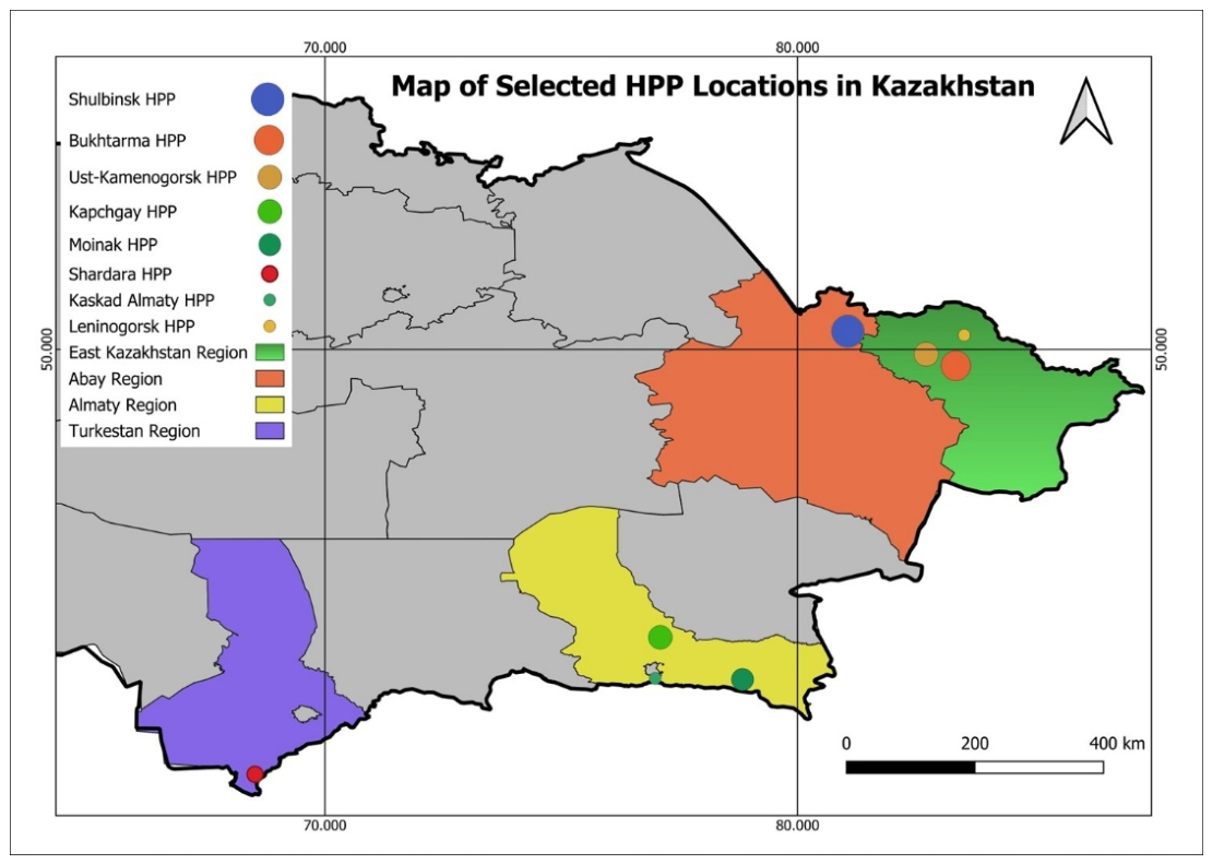
The analysis covers eight hydropower plants (HPPs) in Kazakhstan: Shulbinsk (Shulb), Bukhtarma (Bukh), Ust-Kamenogorsk (Ustk), Leninogorsk (Lenin), Kapchagay (Kapch), Moinak (Moin), Kaskad Almaty (Kask), and Shardara (Shar). These stations represent different hydroclimatic and operational regimes, including large reservoir-based plants, cascade systems, mountain-fed systems, and stations with stronger seasonal variability. As shown in Figure 1, the analyzed HPPs are distributed across hydroclimatically distinct regions of Kazakhstan, which supports station-specific model development. The spatial map in Figure 1 was prepared using QGIS version 3.40.13-Bratislava.

According to official Kazhydromet spring-flood assessments, East Kazakhstan and Abay are classified as higher-risk regions, while Almaty and Turkestan are generally assigned to a medium-risk class at the regional scale [32,33]. The medium regional class, however, does not imply the absence of hazardous hydrological processes. Kazhydromet hydrological forecasts report rain- and snowmelt-driven river-level rises, slope runoff formation, and precipitation-sensitive dynamics in both eastern and southern/southeastern mountain rivers [34,35]. Kazakhstan-based studies further support the hydroclimatic sensitivity of these regions by integrating hydrometeorological monitoring, runoff/indicator mapping, and flood-hazard-oriented analyses at basin and sub-basin scales [36,37,38].

To provide technical and operational context,

Table 1. Installed, available, and restricted capacity for selected HPPs (MW), with commissioning year field for system-context reporting.

Hydropower Plant	Installed (MW)	Available (MW)	No. of Units (Turbines)	Year of Commissioning
Shulbinsk	702.0	702.0	6	1987
Bukhtarma	675.0	675.0	9	1968
Ust-Kamenogorsk	367.8	200.0	4	1952
Leninogorsk	32.0	32	5	1928
Kapchagay	364.0	150.0	4	1970
Moinak	300.0	300.0	2	2011
Kaskad Almaty	46.9	46.9	13	1944
Shardara	126.0	100.0	4	1967

summarizes the main characteristics of the selected HPPs, including installed capacity, available capacity, number of generating units, and commissioning year. These characteristics are relevant because station-specific operating conditions, unit availability, maintenance sensitivity, and regulation capacity can influence the temporal structure of generation and, consequently, forecasting performance.

The target variable is plant-level active power generation, expressed in MW. The raw generation archive covers 2020–2024 at sub-daily operational resolution and was harmonized to an hourly time grid before daily aggregation. Hydro-meteorological predictors include near-surface air temperature, precipitation, and snow water equivalent (SWE), which are physically relevant for inflow formation and generation dynamics in snow-influenced basins. River water-level observations were treated as optional exogenous predictors because their hydrological representativeness and validation contribution differed across stations.

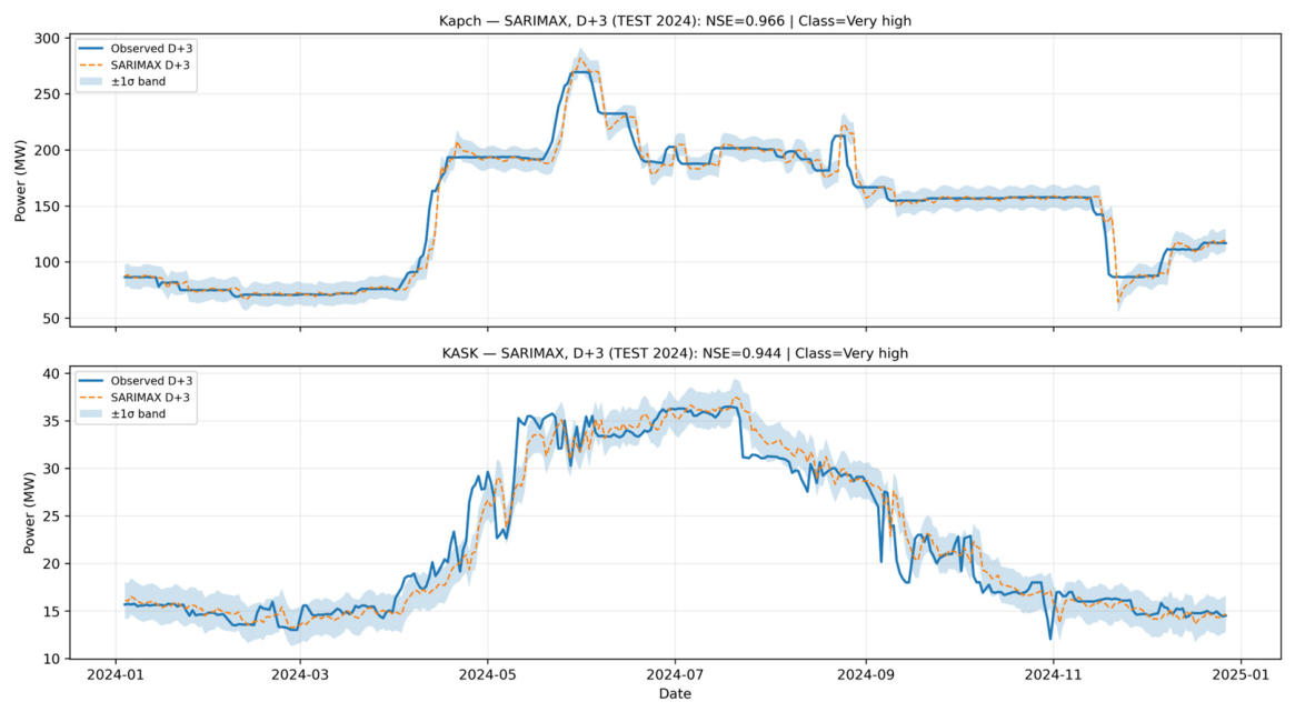
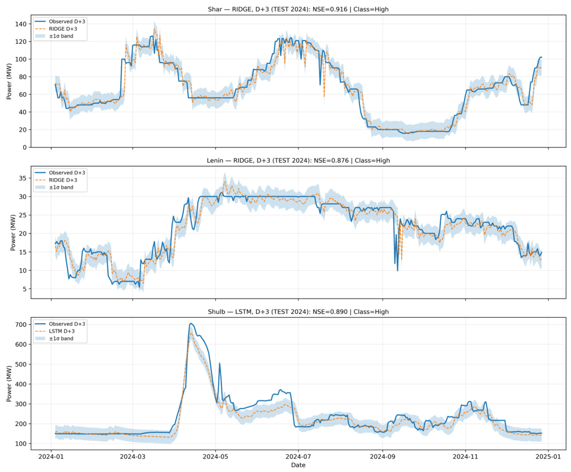
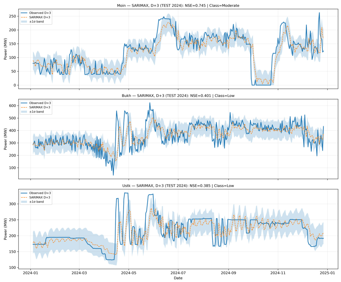
Two forecasting tasks were addressed. The first task is deterministic multi-step forecasting for short operational lead times D+1–D+7, defined as the prediction of daily generation $y_{s,d+h}$ for forecast horizons $h=1,\dots ,7$ from forecast origin $d$ (Equation (1)):

$$y_{\left\{s,d\right\}}^{\left\{\left(k\right)\right\}}=P_{\left\{s,d+k\right\}}, k=1,\dots ,7$$

(1)

where $y_{s,d+h}$ denotes the observed daily generation at station $s$ on target day $d+h$, ${\widehat{y}}_{s,d+h}$ denotes the corresponding forecast, $s$ indicates the station, $d$ is the forecast-origin date, and $h$ is the lead time in days.

The second task is medium-range envelope forecasting for the D+8–D+14 window. Instead of predicting each day in the window separately, this task predicts two window-level descriptors: the minimum generation value and the 90th percentile. For a forecast origin date $d$, the medium-range forecasting window is defined as the set of target days from $d+8$ to $d+14$ (Equation (2)):

$$W_{\left\{s,d\right\}}^{\left\{8:14\right\}}=\{P_{\left\{s,d+8\right\}},P_{\left\{s,d+9\right\}},\dots ,P_{\left\{s,d+14\right\}}\}$$

(2)

The corresponding envelope targets are then defined as the minimum generation within this window, $y_{s,d}^{\mathrm{m}\mathrm{i}\mathrm{n}}$, and the empirical 90th percentile, $y_{s,d}^{q90}$, as given in (Equations (3) and (4)):

$$Y_{s,d}^{MIN}=min\left({\mathcal{W}}_{s,d}^{8:14}\right),$$

(3)

$$Y_{s,d}^{Q90}=Q_{0.90}\left({\mathcal{W}}_{s,d}^{8:14}\right),$$

(4)

where $y_{s,d}^{\mathrm{m}\mathrm{i}\mathrm{n}}$ is the lower-bound target for station $s$ and forecast origin $d$, $y_{s,d}^{q90}$ is the upper-envelope target based on the empirical 90th percentile, and $y_{s,\tau }$ denotes daily generation at station $s$ on day $\tau$. This envelope formulation is intended for medium-range operational planning, where lower-bound and upper-envelope information may be more useful than unstable day-wise point forecasts alone.

To clarify its relationship to probabilistic forecasting, the MIN-Q90 formulation was additionally evaluated using functional-envelope diagnostics. Because MIN and Q90 are future-window descriptors rather than daily calibrated probabilistic intervals, they were assessed as window-level functionals. The diagnostic evaluation therefore included the absolute error of the predicted MIN, the absolute error of the predicted Q90, the error in the predicted envelope width, and the Q90 pinball loss as a quantile-oriented metric for the upper-envelope target. This links the proposed envelope formulation to interval and quantile forecasting concepts while preserving its operational interpretation as a medium-range planning tool rather than a fully calibrated probabilistic forecasting framework.

2.2. Data Harmonization, Quality Control, and Daily Aggregation

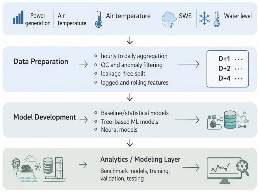
Reliable short-term hydropower forecasting requires input series that are both physically consistent and statistically stable. Raw operational archives collected under heterogeneous logging and reporting practices may contain timestamp inconsistencies, non-physical spikes, negative values, missing values, and telemetry-related artifacts. If untreated, these artifacts can propagate into lagged feature construction, bias model calibration, and distort out-of-sample evaluation. Therefore, a dedicated harmonization and quality-control (QC) pipeline was applied before model training.

The raw table was first standardized by normalizing column names, correcting Cyrillic/Latin character substitutions, harmonizing precipitation labels, and converting numerical fields to floating-point format. The date and time fields were combined into a single datetime index. Records with invalid timestamps were removed, and all remaining observations were sorted chronologically. The dataset was then resampled to an hourly time grid using hourly averaging (Equation (5)):

$$x_{s,h}={\displaystyle \frac{1}{\mid I_h\mid }}{\sum }_{\tau \in I_h}{x}_{s,\tau }^{raw},$$

(5)

where $x_{s,\tau }^{raw}$ is a raw observation for station $s$ at timestamp $\tau$, $x_{s,h}$ is the corresponding hourly value, $h$ is the hourly timestamp, and $I_h$ is the set of raw observations falling within hour $h$. Hourly averaging was used for generation and meteorological descriptors.

Installed capacity was used as a station-specific physical screening bound. Let $P_{s,h}^{raw}$ denote hourly generation at station $s$ and hour $h$, and let $C_s$ denote the installed capacity of station $s$. To allow for minor reporting and rounding deviations, a tolerance factor of 1.05 was applied. Values above 105% of installed capacity and negative generation values were treated as physically implausible and set to missing before imputation (Equation (6)):

$$P_{s,h}^{QC}=\left\{\begin{array}{cc}NaN,& P_{s,h}^{raw}>1.05C_s \mathit{or} P_{s,h}^{raw}<0,\\ P_{s,h}^{raw},& \mathit{otherwise}.\end{array}\right.$$

(6)

where $P_{s,h}^{QC}$ is the quality-controlled hourly generation value, and $\mathrm{N}\mathrm{a}\mathrm{N}$ denotes a missing value introduced either by the original archive or by the QC procedure. Equation (6) prevents physically implausible upward spikes and negative generation artifacts from dominating model fitting and error statistics.

For each station, the QC pipeline recorded the maximum generation before QC, the maximum generation after QC, the number and share of observations exceeding 105% of installed capacity, and the maximum percentage exceedance. Consecutive exceedance runs were also analyzed to distinguish isolated telemetry spikes from longer systematic reporting artifacts. A long exceedance run was defined as a continuous sequence of capacity exceedances lasting more than 24 h, i.e., at least 25 consecutive hourly observations. For each station, the number of long exceedance runs, their total duration, and the maximum run duration were recorded. These diagnostics were not used as model inputs; they were used only to document data quality and ensure preprocessing reproducibility.

After physical screening, missing values were handled using controlled imputation. First, short missing gaps were filled by time-based linear interpolation along the datetime index. Interpolation was restricted to gaps of at most 24 consecutive hours (Equation (7)):

$$P_{s,h}^{int}={Interp}_{time}\left(P_{s,h}^{QC}\right), \mathit{if} \mathit{gap} \mathit{length}\le 24 \mathrm{h},$$

(7)

where $P_{s,h}^{int}$ is the interpolated hourly value and ${\mathrm{I}\mathrm{n}\mathrm{t}\mathrm{e}\mathrm{r}\mathrm{p}}_{time}(\cdot )$ denotes time-based linear interpolation along the datetime index. Equation (7) restores continuity for short telemetry interruptions while avoiding artificial bridging across long outages or structural operational changes.

Remaining missing values were then filled using a rolling median computed over a 7-day window. Since the data are hourly, the window length was as shown in Equation (8):

$$W=7\times 24=168 \mathrm{h},$$

(8)

where $W$ is the rolling-median window length. Boundary values that could not be filled by interpolation or rolling median were filled using forward/backward filling. This final step was used only to avoid edge-related missing values after the main controlled imputation procedure. The number of missing values before QC, after QC, and after imputation was recorded for each station.

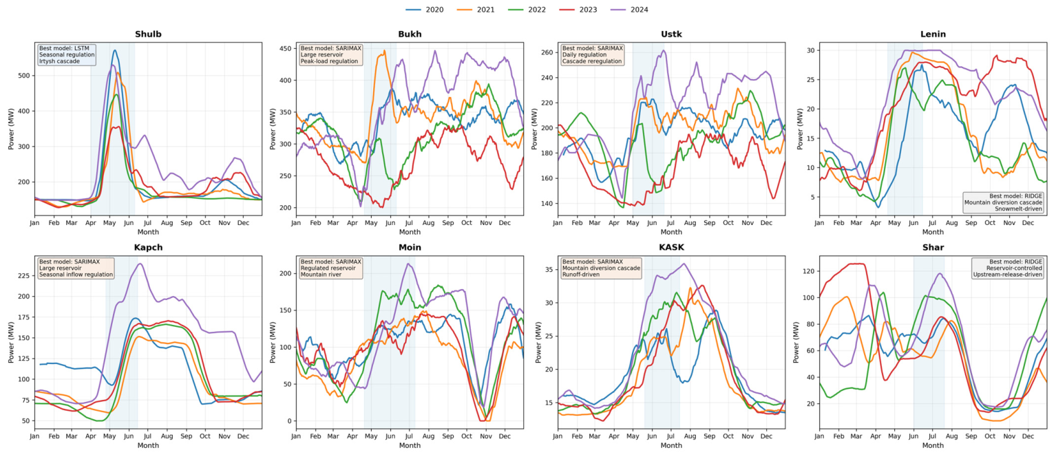
Figure 2 presents the post-QC hourly generation series after physical screening and controlled imputation. The purpose of this figure is both descriptive and diagnostic: it shows that the preprocessing procedure removes non-physical artifacts while preserving station-specific operating regimes, seasonal variability, and genuine low-generation periods.

The final hourly dataset was aggregated to daily resolution for forecasting. Daily generation was computed as the mean of QCed hourly generation values (Equation (9)):

$$P_{s,d}={\displaystyle \frac{1}{24}}{\sum }_{h\in d}{P}_{s,h}^{final},$$

(9)

where $P_{s,d}$ is daily generation for station $s$ on day $d$, and $P_{s,h}^{final}$ denotes the hourly value after QC and imputation. Daily temperature and SWE were treated as state-like descriptors and aggregated using daily averages. Precipitation was aggregated consistently with the harmonized ERA5-derived representation after correcting for replicated sub-daily values. The resulting daily dataset for 2020–2024 was used for all forecasting experiments.

To make the preprocessing auditable, the revised manuscript reports QC diagnostics in the main text, including maximum power before and after QC, number and share of values exceeding 105% of installed capacity, maximum exceedance percentage, long exceedance run diagnostics, NaN counts before QC, NaN counts after QC, and NaN counts after imputation.

2.3. Feature Engineering, Water-Level Ablation, Models, and Evaluation Protocol

For each station, the predictor matrix combined autoregressive generation information with exogenous hydro-meteorological predictors. The base predictor set included daily generation, air temperature, precipitation, and snow water equivalent (SWE). Lagged and rolling features were constructed only from information available at the forecast origin, ensuring that no future observations entered the predictor matrix.

For a base date $d$, the meteorological lag block is represented as $X_{s,d}^{met}$ (Equation (10)):

$${\mathrm{X}}_{s,d}^{met}=[T_{s,d},\dots ,T_{s,d-L+1},R_{s,d},\dots ,R_{s,d-L+1},SW{E}_{s,d},\dots ,SW{E}_{s,d-L+1}],$$

(10)

where $X_{s,d}^{met}$ denotes the meteorological feature block for station $s$ at forecast origin $d$, $T_{s,d-\mathcal{l}}$ denotes daily air temperature, $R_{s,d-\mathcal{l}}$ denotes daily precipitation, $SW{E}_{s,d-\mathcal{l}}$ denotes daily snow water equivalent, $\mathcal{l}=0,\dots ,L-1$ is the lag index, and $L$ is the selected lookback depth. The lookback depth was selected using validation data only. Candidate lookback depths were evaluated on the 2023 validation period, and the final configuration was chosen according to validation NSE. The independent 2024 test period was not used for lookback selection.

The lookback depth was selected through a unified validation-based grid-search procedure. For all model families and all hydropower plants, the same candidate lookback set was evaluated: L = {7, 14, 21, 28, 35} days. This ensured that all models were compared under consistent temporal-search conditions. For each station–model pair, the value of L that achieved the best validation NSE-based performance on the 2023 validation period was selected and then fixed for the independent 2024 test evaluation. The selected lookback depths and the corresponding validation NSE scores are reported in

Table 2. Validation-selected lookback depth L by station and model.

Station	Ridge	RF	HGBR	MLP	LSTM	SARIMAX
Shulb	21 (0.684)	35 (0.658)	35 (0.764)	28 (0.731)	35 (0.740)	21 (0.649)
Bukh	7 (0.195)	14 (0.060)	14 (0.160)	14 (0.236)	35 (0.261)	7 (0.293)
Ustk	21 (0.128)	21 (0.001)	14 (0.039)	14 (0.229)	35 (0.253)	14 (0.331)
Lenin	14 (0.768)	21 (0.776)	21 (0.774)	21 (0.791)	35 (0.809)	35 (0.748)
Kapch	28 (0.977)	14 (0.974)	28 (0.983)	28 (0.967)	21 (0.975)	7 (0.977)
Moin	21 (0.538)	21 (0.547)	35 (0.548)	28 (0.544)	35 (0.554)	7 (0.512)
Kask	7 (0.865)	7 (0.864)	35 (0.861)	14 (0.858)	14 (0.889)	7 (0.875)
Shar	14 (0.939)	7 (0.915)	7 (0.937)	14 (0.945)	28 (0.968)	28 (0.946)

.

For ML/DL models, the selected lookback depth L defined the full historical predictor window used to construct the input matrix. This window included autoregressive generation, air temperature, precipitation, SWE, and the optional water-level input where retained. Therefore, meteorological predictors and autoregressive generation were evaluated within the same candidate historical windows rather than being tuned using separate or inconsistent lag structures.

For SARIMAX, the same candidate lag depths L = {7, 14, 21, 28, 35} were evaluated for the exogenous hydro-meteorological regressors, while the endogenous temporal dependence of daily generation was represented through the selected non-seasonal and seasonal SARIMA orders. Thus, the final configuration for each model was selected using the same validation period and the same candidate lookback range. The selected configuration was then kept unchanged for the independent 2024 test evaluation.

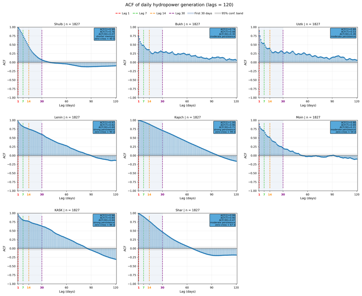
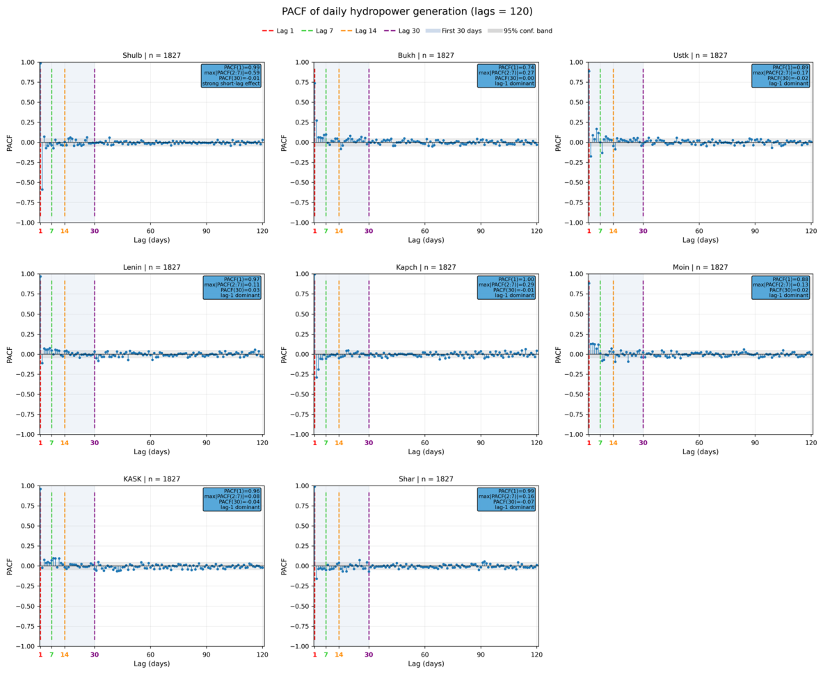
Table 2 shows that the selected memory depth differed both across stations and across model classes. This confirms that a single fixed lookback depth would not be appropriate for the analyzed hydropower system. For example, Kask frequently selected short memory depths of 7–14 days, whereas Shulb, Moin, and several neural network configurations required longer windows of 28–35 days. This variability is consistent with the heterogeneous operating regimes of the stations, including reservoir regulation, cascade effects, mountain-fed runoff, and snow-melt-related seasonal memory. The validation-based selection procedure therefore allowed each station–model pair to use the memory structure that was most informative on the 2023 validation period, while preserving a fully independent 2024 test evaluation.

River water level was treated as an optional exogenous predictor rather than a mandatory input for all stations. This decision was motivated not only by differences in predictive contribution, but also by differences in observational availability and hydrological representativeness. In particular, water-level measurements were not available for all plants from gauging stations located directly within the most relevant river reach controlling the hydropower inflow regime. For several stations, no hydrological post was available at the required hydraulic section, and the closest available regional gauging station had to be used as a proxy. Consequently, the informative value of water-level observations was expected to vary across stations depending on gauge placement, river regulation effects, and the degree to which the selected gauge reflected local hydrological conditions at the plant.

Where available, water-level series were collected over the full 2020–2024 study period and incorporated into the candidate predictor pool. However, to avoid test-driven feature selection, the decision to retain or exclude water level was made exclusively using the 2023 validation period. For each station, two otherwise identical configurations were compared: $M_0$, a model without water level, and $M_1$, a model with water level. The validation gain from water-level inclusion was computed as $\mathsf{\Delta }NS{E}_s$ (Equation (11)):

$$\mathsf{\Delta }NS{E}_s=NS{E}_s^{WL}-NS{E}_s^{NoWL},$$

(11)

where $\mathsf{\Delta }NS{E}_s$ denotes the validation gain for station $s$, $NS{E}_s^{WL}$ is the validation NSE obtained when the water level is included, and $NS{E}_s^{NoWL}$ is the validation NSE obtained without the water level.

The water level was retained only when ΔNSE > 0.01. This threshold was introduced to avoid adding an extra exogenous predictor when the validation gain was negligible or likely attributable to numerical noise. The corresponding station-specific validation results and final USE/DROP decisions are summarized in

Table 3. Validation-based ablation test for water-level inclusion. Validation NSE was computed on the 2023 validation period.

Station	NSE_no_wl	NSE_with_wl	Delta	Decision
Shulb	0.683	0.682	−0.0006	DROP
Bukh	0.083	0.192	0.1091	USE
Ustk	0.128	0.107	−0.0208	DROP
Lenin	0.758	0.464	−0.2935	DROP
Kapch	0.976	0.978	0.0015	DROP
Moin	0.526	0.538	0.0120	USE
Kask	0.802	0.851	0.0493	USE
Shar	0.933	0.920	−0.0123	DROP

. The independent 2024 test period was not used for this decision.

To keep the feature selection procedure transparent, leak-free, and comparable across models, water-level ablation was performed once on the 2023 validation period using Ridge regression (or Tikhonov regularization) as a parsimonious regularized linear reference model [39,40]. The resulting station-specific USE/DROP decision was then fixed and applied consistently to all downstream models. In this way, water-level inclusion was treated as a validation-based feature-selection step rather than as a model-specific hyperparameter, thereby avoiding unequal tuning effort across methods and preserving a fair comparison on the independent 2024 test set.

The ablation results show that water level was not uniformly beneficial across stations. A positive and practically meaningful validation gain was observed for Bukhtarma ($\mathsf{\Delta }NSE=+0.109$), Moinak ($\mathsf{\Delta }NSE=+0.012$), and Kaskad Almaty ($\mathsf{\Delta }NSE=+0.049$); therefore, water level was retained for these stations. For Shulbinsk, Ust-Kamenogorsk, Leninogorsk, and Shardara, including water level reduced validation NSE. For Kapchagay, the gain was positive but negligible ($\mathsf{\Delta }NSE=+0.002$) and below the predefined threshold; therefore, water level was not retained.

This station-specific behavior is physically plausible. In regulated hydropower systems, generation is not determined by river stage alone. It also depends on dispatch decisions, turbine availability, reservoir operation, cascade coordination, and plant-specific constraints. Therefore, a water-level gauge provides useful information only when it is sufficiently representative of the hydrological conditions controlling generation at a given plant. In other stations, water level may be redundant with autoregressive generation features, weakly synchronized with the target, affected by regulation, or too noisy to improve validation performance. For this reason, enforcing water level as a universal predictor would reduce model robustness and make the comparison less meaningful.

The model set included representative linear, statistical, tree-based, and neural approaches: Linear Regression (LR), SARIMAX, Random Forest (RF), Histogram Gradient Boosting Regressor (HGBR), Multilayer Perceptron (MLP), and Long Short-Term Memory (LSTM). In the revised experiments, operational baseline was also included to strengthen the interpretation of model skill. The Persistence baseline was defined as the most recent available daily generation value at the forecast origin (Equation (12)):

$${\widehat{P}}_{s,d+k}^{pers}=P_{s,d},$$

(12)

where ${\widehat{y}}_{s,d+h}^{pers}$ denotes the Persistence forecast for station $s$, forecast origin $d$, and lead time $h$, and $y_{s,d}$ is the observed daily generation at the forecast origin.

All experiments followed a strict chronological split: 2020–2022 for training, 2023 for validation and model selection, and 2024 for independent testing. Hyperparameters, lookback depth, water-level inclusion, and model-selection decisions were made exclusively on the validation period. After selection, final models were retrained on the combined training and validation data and evaluated once on the independent 2024 test period. This design prevents data leakage and approximates real operational deployment conditions.

Model performance was evaluated using Nash–Sutcliffe efficiency (NSE), root mean squared error (RMSE) and mean absolute error (MAE). NSE was computed as in Equation (13):

$$NSE=1-{\displaystyle \frac{{\displaystyle {\sum }_{i=1}^n}(y_i-{\widehat{y}}_i{)}^2}{{\displaystyle {\sum }_{i=1}^n}(y_i-\overline{y}{)}^2}},$$

(13)

where $y_i$ is the observed value, ${\widehat{y}}_i$ is the predicted value, $\overline{y}$ is the mean observed value over the evaluation sample, and $n$ is the number of evaluated samples.

RMSE and MAE were computed as in Equations (14) and (15):

$$RMSE=\sqrt{{\displaystyle \frac{1}{n}}{\displaystyle {\sum }_{i=1}^n}(y_i-{\widehat{y}}_i{)}^2},$$

(14)

and:

$$MAE={\displaystyle \frac{1}{n}}{\displaystyle {\sum }_{i=1}^n}\mid y_i-{\widehat{y}}_i\mid .$$

(15)

NSE was used as the primary performance metric because it is widely used in hydrological forecasting and provides an efficiency-based measure relative to the variance in the observed series. RMSE and MAE were reported alongside NSE to preserve engineering interpretability in MW.

2.4. Performance Uncertainty and Statistical Comparison

To quantify the uncertainty of the reported test-period metrics, an additional performance variability analysis was conducted for the D+1–D+7 forecasting task. Because the 2024 test predictions form temporally ordered and partially overlapping multi-step forecast sequences, individual forecast samples were not treated as independent. Instead, a moving-block bootstrap was applied over forecast-origin dates using 14-day blocks. For each bootstrap replicate, NSE, RMSE, and MAE were recomputed over the pooled D+1–D+7 test predictions. The 95% confidence intervals were obtained from the 2.5th and 97.5th percentiles of the bootstrap distributions.

In addition, rolling-window metrics were computed over the 2024 test period using 30-day windows shifted weekly. The standard deviation of rolling-window NSE, RMSE, and MAE was used to quantify within-year variability in model performance. Finally, paired moving-block bootstrap comparisons were performed for key model contrasts. For NSE, a positive difference indicates that the first model performs better; for RMSE and MAE, a negative difference indicates improvement. Differences were interpreted as statistically robust when the 95% bootstrap confidence interval did not overlap zero.

The overall experimental workflow is summarized in Figure 3. It consists of raw data harmonization, physical QC and controlled imputation, daily aggregation, feature construction, validation-based lookback and water-level selection, model training and hyperparameter tuning, and final independent testing. This design ensures that the reported results are based on a reproducible and leakage-safe forecasting protocol.

3. Results

This section reports out-of-sample forecasting results on the independent 2024 test period. The analysis covers eight hydropower plants with complete model outputs across all lead times: Shulbinsk (Shulb), Bukhtarma (Bukh), Ust-Kamenogorsk (Ustk), Leninogorsk (Lenin), Kapchagay (Kapch), Moinak (Moin), Kaskad Almaty (Kask), and Shardara (Shar). The results are presented in three steps. First, we summarize short-horizon performance over D+1–D+7 using the station-wise best model and compare it against the Persistence baseline. Second, we interpret the updated D+3 trajectory plots by forecastability regime. Third, we present the switched-hybrid results for Ust-Kamenogorsk and the medium-range envelope forecasting results for D+8–D+14.

Across all station–horizon combinations, predictive skill decreased with increasing lead time, as expected for multi-step hydropower forecasting. However, the rate of degradation was strongly station-dependent, indicating substantial heterogeneity in short-term forecastability across Kazakhstan’s hydropower plants.

3.1. Short-Horizon Performance (D+1 to D+7)

3.1.1. Cross-Model Performance Patterns

To summarize the short-horizon benchmark,

Table 4. Station-wise summary of the best short-horizon forecasting results (TEST 2024, D+1–D+7).

Station	Best Model	Mean NSE (D+1–D+7)	Mean NSE (Persistence)	NSE D+7	NSE D+7 (Persistence)	Class
Kapch	SARIMAX	0.941	0.938	0.874	0.862	Very high
Kask	SARIMAX	0.933	0.928	0.898	0.875	Very high
Shar	RIDGE	0.893	0.886	0.812	0.790	High
Lenin	RIDGE	0.854	0.831	0.780	0.755	High
Shulb	LSTM	0.848	0.793	0.732	0.598	High
Moin	SARIMAX	0.698	0.672	0.533	0.494	Moderate
Bukh	SARIMAX	0.411	0.139	0.329	−0.084	Low
Ustk	SARIMAX	0.362	0.209	0.145	−0.059	Low

reports the best-performing model for each station together with the mean NSE over D+1–D+7 and the corresponding NSE at D+7. The mean NSE is used as the primary summary metric because the forecasting task is explicitly multi-step and should be evaluated over the full weekly horizon rather than at a single lead time.

Table 4 shows substantial cross-station heterogeneity in forecastability. Kapchagay and Kaskad Almaty form the strongest group, with very high mean skill maintained up to D+7. Shardara, Leninogorsk, and Shulbinsk also remain reliably predictable, although with more visible horizon-wise degradation. In contrast, Moinak, Bukhtarma, and Ust-Kamenogorsk show lower robustness, indicating that forecast uncertainty grows more rapidly at these plants. Overall, the results confirm that short-term hydropower forecasting performance in Kazakhstan is strongly station-dependent, and that the best model is not uniform across all operational regimes.

The same table also reveals three forecastability regimes. Kapch and Kask belong to the very high class, with very strong mean NSE and high skill preserved even at D+7. Shar, Lenin, and Shulb form the high class, where short-horizon forecasts remain reliable but degradation with horizon is more visible. Moin belongs to the moderate class, while Bukh and Ustk fall into the low class, where uncertainty grows substantially toward weekly lead times. This grouped interpretation is more informative than a station-by-station list because it shows that forecast behavior clusters into broad operational patterns rather than following a single national-level regime.

In terms of model choice, the revised benchmark does not support a universal winner across all stations. SARIMAX remains the best-performing model for Kapch, Kask, Moin, Bukh, and Ustk, RIDGE is best for Shar and Lenin, and LSTM performs best for Shulb. This result reinforces the station-wise logic of this study: model preference depends on the local hydro-operational regime rather than on model family alone.

Figure 4, Figure 5 and Figure 6 present the D+3 observed-versus-predicted trajectories for the best model at each station, with an uncertainty band shown as ±1 standard deviation around the predicted series. These figures complement

Table 5. NSE summary for the very-high-forecastability class (best model per station, TEST 2024).

Station	Best Model	NSE D+1	NSE D+3	NSE D+5	NSE D+7	Mean NSE (D+1–D+7)	NSE Decline (D+1→D+7)
Kapch	SARIMAX	0.994	0.967	0.924	0.874	0.942	0.121
Kask	SARIMAX	0.979	0.944	0.918	0.898	0.933	0.081

by showing how forecast behavior changes across the forecastability regimes.

The very-high-forecastability class includes Kapch and Kask, both best represented by SARIMAX (Table 5). As shown in Figure 4, the predicted D+3 trajectories follow the observed generation closely throughout the year, and the uncertainty bands remain relatively narrow.

This visual behavior is consistent with the high mean NSE values and the limited loss of skill at D+7 reported in Table 5. Operationally, these stations are suitable for weekly planning with relatively modest uncertainty growth.

The high-forecastability class includes Shar, Lenin, and Shulb (

Table 6. NSE summary for the high-forecastability class (best model per station, TEST 2024).

Station	Best Model	NSE D+1	NSE D+3	NSE D+5	NSE D+7	Mean NSE (D+1–D+7)	NSE Decline (D+1→D+7)
Shar	RIDGE	0.967	0.916	0.871	0.812	0.893	0.156
Lenin	RIDGE	0.944	0.876	0.820	0.780	0.854	0.165
Shulb	LSTM	0.945	0.890	0.818	0.732	0.848	0.213

). In this group, the D+3 trajectories in Figure 5 still show good agreement between observed and predicted generation, but the uncertainty bands are wider and local deviations become more visible than in the very high class.

Shar and Lenin are best captured by Ridge, whereas Shulb is best represented by LSTM, as summarized in Table 6. This result is important because it shows that the best model need not be identical even within the same forecastability class. These plants remain operationally predictable, but uncertainty should be acknowledged more explicitly beyond the shortest horizons.

The moderate/low-forecastability group includes Moin, Bukh, and Ustk, all best represented by SARIMAX (

Table 7. NSE summary for the moderate/low-forecastability class (best model per station, TEST 2024).

Station	Best Model	NSE D+1	NSE D+3	NSE D+5	NSE D+7	Mean NSE (D+1–D+7)	NSE Decline (D+1→D+7)
Moin	SARIMAX	0.888	0.745	0.638	0.533	0.698	0.355
Bukh	SARIMAX	0.642	0.401	0.313	0.329	0.411	0.313
Ustk	SARIMAX	0.834	0.385	0.180	0.145	0.362	0.685

). As illustrated in Figure 6, the D+3 plots show much larger dispersion and visibly wider uncertainty bands than in the other two regimes.

At Ustk in particular, the mismatch between smoother model dynamics and high-variability periods becomes more apparent, which is consistent with the lower mean NSE and weaker D+7 performance reported in Table 7. This class therefore provides the strongest motivation for targeted methodological refinement, since the baseline short-horizon setup captures only part of the observed variability.

3.1.2. Flood-Sensitive Switched Hybrid Strategy for Ust-Kamenogorsk

To address the weakest station-level behavior observed in the standard D+1–D+7 setup, we introduced a flood-sensitive switched hybrid strategy for Ust-Kamenogorsk (Ustk). The aim was not to replace the station-wise benchmark globally, but to test whether forecast robustness could be improved during the spring high-variability period while preserving stable behavior outside it.

Ustk is an appropriate test case because it shows comparatively low short-horizon robustness in the baseline setting together with strong seasonal sensitivity. In such systems, inflow variability, operational constraints, and dispatch decisions may weaken the assumptions behind a single-regime forecasting model. The switched hybrid therefore separates a calm branch and a flood-sensitive branch and activates them according to an observed-generation high-flow window selected by a regime-score procedure.

To make the seasonal activation window quantitative, the broader spring search season was defined as 15 March–15 June. For each year in the selection period of 2020–2023, high-flow days and peak days were identified from observed daily generation using the 75th and 90th percentiles of spring generation, respectively. Candidate calendar windows were then ranked by a regime score that combined high-flow coverage, peak-day coverage, minimum year-wise coverage, and a length penalty to avoid unnecessarily wide activation periods. The resulting selection diagnostics are summarized in

Table 8. Observed-generation regime-score selection of the Ust-Kamenogorsk spring high-flow window.

Indicator	Value
Selection years	2020–2023
Spring search season	15 March–15 June
Selected high-flow window	5 April–15 June
Window length	72 days
Regime score	96.085
High-flow coverage	95.833%
Peak-day coverage	100.000%
Minimum yearly high-flow coverage	83.333%
Years with high-flow coverage ≥ 70%	4/4
Years with peak-day coverage ≥ 70%	4/4
Mean generation inside window	181.708 MW
Q90 generation inside window	251.846 MW
Maximum generation inside window	271.208 MW

. This procedure selected 5 April–15 June as the spring high-flow window for Ust-Kamenogorsk.

This experiment was intentionally limited to Ustk. It is presented as a targeted methodological extension for a difficult station rather than as a universal replacement for the full benchmark.

From the hourly QC data, we constructed daily predictors using the same aggregation logic as in the main pipeline, namely daily means for most variables and daily sums for precipitation. Two daily targets were defined as follows (Equation (16)):

$$y_d^{\mathrm{mean}}={\displaystyle \frac{1}{24}}{\displaystyle \sum _{h=1}^{24}}{P}_{d,h},y_d^{\max }=\underset{h\in \{1,\dots ,24\}}{\mathrm{m}\mathrm{a}\mathrm{x}}{P}_{d,h}.$$

(16)

For each base date $t$, multi-output samples (Equation (17)) were formed for horizons $h=1,\dots ,7$ (Equation (17)):

$${\mathrm{y}}_t^{\mathrm{mean}}=\left(y_{t+1}^{\mathrm{mean}},\dots ,y_{t+7}^{\mathrm{mean}}\right),{\mathrm{y}}_t^{\max }=\left(y_{t+1}^{\max },\dots ,y_{t+7}^{\max }\right)$$

(17)

Let ${\mathbf{z}}_t$ denote the daily feature vector (generation, temperature, precipitation, SWE, and optional water-level term with lag). With lookback $L$, the input is as shown in Equation (18):

$${\mathrm{X}}_t=\left[{\mathrm{z}}_{t-L+1},\dots ,{\mathrm{z}}_t\right]$$

(18)

A flood-window indicator is defined for each target day (Equation (19)):

$$I_{t+h}^{\mathit{flood}}=\left\{\begin{array}{cc}1,& \mathit{if} \mathit{date}(t+h)\in \left[5 \mathit{April}, 15 \mathit{June}\right]\\ 0,& \mathit{otherwise}\end{array}\right.$$

(19)

and the final prediction is as shown in Equation (20):

$${\widehat{y}}_{t+h}^{\mathrm{sw}}=\left(1-I_{t+h}^{\mathrm{flood}}\right){\widehat{y}}_{t+h}^{\mathrm{base}}+I_{t+h}^{\mathrm{flood}}{\widehat{y}}_{t+h}^{\mathrm{flood}}$$

(20)

Thus, the switching rule is purely calendar-based in the present implementation: predictions for days outside the spring flood window are taken from the base branch, whereas predictions for days inside the flood window are taken from the flood-sensitive branch.

Using the observed-regime-selected high-flow window, the switched hybrid strategy improved forecast robustness at Ustk across the full D+1–D+7 range, with the largest gains at medium-to-long lead times where spring variability most strongly degrades single-regime forecasts. For the RIDGE backbone, ΔNSE increased from +0.035 at D+1 to +0.343 at D+6, while RMSE and MAE were reduced by 29.7–39.3% and 26.8–28.4%, respectively (

Table 9. Ustk results for RIDGE: BASE vs. SWITCHED using the observed-regime-selected high-flow window, TEST 2024.

Horizon	BASE NSE	SWITCHED NSE	BASE RMSE	SWITCHED RMSE	BASE MAE	SWITCHED MAE
D+1	0.819	0.854	18.697	13.138	11.545	8.428
D+2	0.549	0.701	29.470	18.738	19.155	13.785
D+3	0.346	0.590	35.472	21.895	23.462	16.803
D+4	0.200	0.513	39.189	23.835	26.295	18.848
D+5	0.135	0.474	40.704	24.723	27.547	19.766
D+6	0.117	0.460	41.097	25.023	27.925	20.132
D+7	0.109	0.435	41.250	25.540	28.437	20.805

). For the SARIMAX backbone, the same pattern was even more pronounced: ΔNSE reached +0.407 at D+6, with RMSE and MAE reductions of 30.2–44.5% and 28.6–35.5%, respectively (

Table 10. Ustk results for SARIMAX: BASE vs. SWITCHED using the observed-regime-selected high-flow window, TEST 2024.

Horizon	BASE NSE	SWITCHED NSE	BASE RMSE	SWITCHED RMSE	BASE MAE	SWITCHED MAE
D+1	0.834	0.867	18.012	12.576	10.364	7.402
D+2	0.587	0.739	28.317	17.551	17.335	11.755
D+3	0.387	0.644	34.466	20.426	21.316	14.105
D+4	0.256	0.602	37.941	21.599	23.536	15.184
D+5	0.190	0.578	39.541	22.183	24.393	15.795
D+6	0.171	0.578	39.950	22.156	24.271	15.741
D+7	0.161	0.559	40.167	22.609	24.663	16.221

).

The fact that both Ridge and SARIMAX benefit from the same observed-regime-selected switching logic suggests that the main source of improvement is regime decomposition rather than learner-specific tuning. In other words, the gain arises primarily from separating calm and high-flow behavior, not merely from changing the forecasting model itself.

This interpretation is also supported by the updated figures. As shown in Figure 7, the switched forecasts follow the high-variability spring trajectories more closely than the corresponding base models. In turn, Figure 8 shows that the switched strategy yields consistent horizon-wise gains, especially from D+3 onward, when the limitations of the single-regime setup become more apparent.

3.1.3. Generalized Cross-Station Performance Analysis

The cross-station comparison of forecasting models over the TEST 2024 period (D+1–D+7) reveals stable and interpretable performance patterns across heterogeneous hydropower operating regimes. To provide an aggregated view, mean Nash–Sutcliffe efficiency (NSE) values were computed across all analyzed stations (Shulbinsk, Bukhtarma, Ust-Kamenogorsk, Leninogorsk, Kapchagay, Moinak, Kaskad Almaty, and Shardara) for each model and forecast horizon.

At short lead times, the strongest aggregated performance in the present benchmark is provided by the parsimonious statistical models. SARIMAX achieves the highest mean NSE at D+1 (0.903), while Ridge remains highly competitive throughout the full D+1–D+7 range and slightly exceeds SARIMAX from D+5 onward. This result indicates that, for the analyzed stations and evaluation period, regularized linear and seasonal autoregressive approaches remain strong operational choices for short-term hydropower forecasting.

As expected, forecasting skill decreases monotonically with increasing horizon for all methods. However, the rate of degradation differs by model class. From D+1 to D+7, the mean NSE decline is 0.271 for Ridge and 0.284 for SARIMAX, compared with 0.372 for HGBR and 0.357 for Persistence (

Table 11. Mean NSE by forecast horizon (D+1–D+7) across all analyzed hydropower stations (TEST 2024).

Horizon	HGBR	Ridge	LSTM	MLP	RF	SARIMAX	PERSIST
D+1	0.842	0.896	0.810	0.764	0.763	0.903	0.891
D+2	0.746	0.819	0.739	0.700	0.684	0.831	0.813
D+3	0.645	0.753	0.678	0.659	0.624	0.763	0.721
D+4	0.584	0.707	0.638	0.610	0.582	0.712	0.650
D+5	0.532	0.674	0.614	0.574	0.550	0.674	0.589
D+6	0.497	0.650	0.590	0.557	0.527	0.647	0.558
D+7	0.470	0.625	0.562	0.521	0.500	0.619	0.534

). LSTM, MLP, and RF show intermediate declines of 0.248, 0.243, and 0.263, respectively. These results indicate that no model family is universally dominant across all horizons and that the strongest aggregate performance in this benchmark is concentrated mainly in Ridge and SARIMAX.

The aggregated comparison also clarifies the role of model class in the present benchmark. Neural and tree-based approaches achieved competitive results for selected stations and horizons, but the strongest aggregate D+1–D+7 performance was obtained by Ridge and SARIMAX. For the analyzed stations, predictors, and the 2020–2024 evaluation period, increased model complexity alone was not a reliable indicator of higher operational forecasting skill.

Station-specific feature design also contributed to the final performance patterns. In particular, lag-0 water-level input was retained only for Bukhtarma, Moinak, and Kaskad Almaty, where the validation-based ablation results in Table 3 showed meaningful improvements in NSE. For the remaining stations, water level was excluded because its contribution was negligible and/or sufficiently continuous observations were unavailable. These results indicate that uniform feature enforcement across all plants would not have been appropriate.

For visualization, the aggregated trend is shown in Figure 9 as mean NSE versus forecast horizon. This representation makes the horizon-wise decline directly visible and highlights the relative robustness of the strongest models under weekly forecasting conditions.

3.1.4. Performance Uncertainty and Statistical Robustness

To complement the point estimates reported above, the pooled D+1–D+7 test predictions were additionally evaluated using moving-block bootstrap confidence intervals, rolling-window variability, and paired bootstrap comparisons. This analysis was performed across all analyzed stations and forecast horizons to quantify the stability of the reported metrics over the 2024 test period and to avoid interpreting small point-estimate differences as definitive model rankings.

First, moving-block bootstrap confidence intervals were computed for the pooled D+1–D+7 NSE, RMSE, and MAE values. The results are summarized in

Table 12. Moving-block bootstrap confidence intervals for pooled D+1–D+7 test metrics across all analyzed stations.

Model	NSE	NSE 95% CI	RMSE	RMSE 95% CI	MAE	MAE 95% CI
RIDGE	0.920	[0.894, 0.945]	36.161	[28.728, 44.791]	18.463	[15.824, 21.835]
SARIMAX	0.918	[0.885, 0.946]	36.626	[28.155, 46.153]	17.397	[14.476, 21.282]
LSTM	0.903	[0.879, 0.921]	39.786	[33.702, 47.481]	21.969	[18.835, 26.568]
Persistence	0.896	[0.850, 0.935]	41.200	[30.766, 52.122]	17.553	[14.278, 21.909]
HGBR	0.890	[0.852, 0.921]	42.236	[34.079, 52.634]	22.555	[18.832, 27.989]
RF	0.886	[0.859, 0.912]	43.031	[35.849, 51.781]	24.498	[20.711, 29.899]
MLP	0.878	[0.842, 0.911]	44.555	[35.312, 54.218]	24.022	[19.520, 28.799]

. This table provides the point estimate for each model together with the corresponding 95% confidence interval, allowing the uncertainty of the aggregated model comparison to be assessed directly.

Table 12 confirms that RIDGE and SARIMAX form the strongest performance group in the pooled D+1–D+7 evaluation. Their NSE confidence intervals overlap substantially, indicating that the small difference between their point estimates should not be interpreted as a statistically decisive ranking. Both models, however, show higher point NSE and lower RMSE than Persistence. LSTM remains competitive, but its pooled NSE is lower than those of RIDGE and SARIMAX. Therefore, the model ranking should be interpreted conservatively, with emphasis on robust model groups rather than a single universal winner.

Second, rolling-window metrics were computed to assess within-year variability over the 2024 test period. The corresponding rolling-window means and standard deviations are reported in

Table 13. Rolling-window variability in pooled D+1–D+7 performance over the 2024 test period.

Model	Rolling NSE Mean	Rolling NSE SD	Rolling RMSE Mean	Rolling RMSE SD	Rolling MAE Mean	Rolling MAE SD
SARIMAX	0.923	0.059	33.378	16.876	17.715	8.081
RIDGE	0.923	0.046	33.949	14.657	18.890	7.095
LSTM	0.906	0.041	38.084	14.153	22.539	8.136
Persistence	0.903	0.076	37.300	19.547	17.890	9.343
HGBR	0.897	0.061	39.511	17.746	23.305	10.627
RF	0.892	0.061	40.606	17.255	25.323	11.184

. This analysis complements the bootstrap confidence intervals by showing how model performance varies across different parts of the test year.

As shown in Table 13, performance variability within 2024 was non-negligible. Persistence had the largest rolling NSE standard deviation, indicating stronger sensitivity to within-year regime changes. RIDGE and LSTM had the lowest rolling NSE variability among the strongest learned models, while SARIMAX achieved the highest rolling mean NSE together with moderate variability. These results support the interpretation that point metrics should be read together with uncertainty estimates rather than as fixed deterministic rankings.

Third, paired moving-block bootstrap comparisons were conducted for the key model contrasts. The results are shown in

Table 14. Paired moving-block bootstrap comparisons for key model contrasts.

Model	ΔNSE	95% CI	p-Value	Interpretation
RIDGE−Persistence	0.024	[0.002, 0.046]	0.04	robust NSE improvement
SARIMAX−Persistence	0.022	[0.010, 0.038]	<0.01	robust NSE improvement
LSTM−Persistence	0.007	[−0.024, 0.040]	0.86	not robust
SARIMAX−RIDGE	−0.002	[−0.013, 0.011]	0.85	not robust
SARIMAX−LSTM	0.015	[−0.005, 0.035]	0.20	not robust
RIDGE−LSTM	0.017	[0.005, 0.029]	<0.01	robust NSE improvement

. Positive ΔNSE values indicate that the first model has higher NSE than the second model. A difference was interpreted as robust only when the 95% confidence interval did not cross zero.

Based on the station-level and aggregated evidence, four practical conclusions follow:

• Forecastability is strongly station-dependent, and model performance should therefore be interpreted at the plant level rather than only through a single aggregated ranking.
• Parsimonious models remain highly competitive under the evaluated operational conditions. In the present benchmark, Ridge and SARIMAX provide the strongest and most stable overall performance across the D+1–D+7 horizon.
• Model complexity alone is not a reliable indicator of forecasting accuracy. Tree-based and neural models are competitive in selected station- and horizon-specific cases, but they do not provide a consistent aggregate advantage over Ridge and SARIMAX in the present dataset.
• Persistence remains a relevant operational baseline, particularly at short horizons and at more regular stations. However, the strongest forecasting models generally provide better average weekly skill, especially at more variable stations.

3.2. Medium-Range Envelope Forecasting (D+8–D+14)

To assess whether useful predictability persists beyond the weekly horizon, envelope forecasting was performed for the D+8–D+14 window using two targets: MIN, representing a conservative lower bound, and Q90, representing an upper operational quantile. In line with the forecastability grouping introduced in Section 3.1, this experiment was restricted to the stations with stronger short-range performance, namely the very high class (Kapch, Kask) and the high class (Shar, Lenin, Shulb).

In the revised analysis, the D+8–D+14 envelope-forecasting benchmark includes MLP, LSTM, HGBR, RF, RIDGE, and SARIMAX. The overall cross-model results are summarized in

Table 15. Mean envelope forecasting metrics across the selected stations for D+8–D+14 (TEST 2024).

Model	Mean MIN NSE	Mean Q90 NSE	Mean MIN NSE (Persistence)	Mean Q90 NSE (Persistence)
MLP	0.533	0.686	0.556	0.653
LSTM	0.592	0.746	0.556	0.653
HGBR	0.417	0.601	0.556	0.653
RF	0.500	0.637	0.556	0.653
RIDGE	0.658	0.743	0.556	0.653
SARIMAX	0.664	0.676	0.556	0.653

and Figure 10 to provide a compact comparison across all evaluated methods. This study then discusses SARIMAX and RIDGE in greater detail because these parsimonious models are central to methodological interpretation and provide an operationally transparent reference for medium-range envelope forecasting.

As shown in Table 15, all reported mean NSE values remain positive, indicating retained medium-range predictability in the selected very high/high subset. For the MIN target, the strongest average performance is obtained by SARIMAX (0.664) and RIDGE (0.658). For the Q90 target, the strongest mean results are achieved by LSTM (0.746) and RIDGE (0.743), whereas SARIMAX (0.676) remains competitive but is less robust than RIDGE for the upper-envelope target. The Persistence baseline remains relevant, but it is generally matched or exceeded by at least one learned model in the aggregated comparison.

To clarify the relationship between the D+8–D+14 envelope formulation and probabilistic forecasting, an additional functional-envelope diagnostic analysis was performed. Since the proposed MIN and Q90 outputs are future-window descriptors rather than daily calibrated probabilistic intervals, they were evaluated as window-level functionals. Specifically, we assessed the absolute error of the predicted MIN, the absolute error of the predicted Q90, the error in the predicted envelope width, and the Q90 pinball loss as a quantile-oriented diagnostic. This analysis links the proposed envelope formulation to interval and quantile forecasting concepts while preserving its operational interpretation as a medium-range planning tool.

Since the D+8–D+14 experiment is formulated as window-functional envelope forecasting, its uncertainty was evaluated using diagnostics aligned with this target structure rather than by applying the same daily paired testing framework used for D+1–D+7. These diagnostics complement the formal D+1–D+7 bootstrap analysis by assessing the stability and quantile-oriented behavior of the medium-range envelope outputs.

The functional-envelope diagnostics in

Table 16. Functional-envelope diagnostics for the D+8–D+14 window on the 2024 test period.

Model	MIN MAE (MW)	Q90 MAE (MW)	Width MAE (MW)	Q90 Pinball Loss	Functional MAE Mean (MW)
SARIMAX	14.834	17.583	9.512	9.597	16.208
LSTM	16.560	15.996	9.511	9.579	16.278
RIDGE	16.592	18.777	9.955	10.470	17.685
RF	19.325	20.622	9.324	13.294	19.973
MLP	20.424	20.824	11.913	11.439	20.624
HGBR	22.719	24.106	10.837	16.056	23.413

support the interpretation of the D+8–D+14 task as an operational envelope-forecasting problem. Among the evaluated models, SARIMAX provides the strongest overall functional accuracy, with the lowest combined MIN/Q90 error. LSTM achieves the lowest Q90 MAE and the lowest Q90 pinball loss, indicating strong upper-envelope behavior. RIDGE remains competitive and provides a stable parsimonious alternative, although its functional errors are slightly higher than those of SARIMAX and LSTM.

The remaining models, RF, MLP, and HGBR, also retain informative envelope-forecasting behavior but show larger functional errors, especially for the Q90 target. This confirms that medium-range envelope forecasting remains model-dependent and target-dependent. Importantly, the functional diagnostics provide a clearer link to quantile-oriented forecasting: Q90 is evaluated as an upper-envelope quantile-like target using both absolute error and pinball loss. However, the method should not be interpreted as a fully calibrated probabilistic forecast, because no complete predictive distribution is estimated. Instead, the approach provides operationally interpretable lower-bound and upper-envelope descriptors for medium-range planning.

The station-wise comparison across all evaluated models is summarized in Figure 10, which shows that the medium-range ranking is not uniform across stations or targets. This confirms that envelope forecasting for D+8–D+14 remains both station-specific and target-specific.

The observed and predicted envelope trajectories for SARIMAX are shown in Figure 11, and the corresponding station-level metrics are summarized in

Table 17. Envelope metrics for SARIMAX, D+8–D+14 (TEST 2024).

Station	MIN RMSE	MIN MAE	MIN NSE	Q90 RMSE	Q90 MAE	Q90 NSE
Shulb	71.482	41.430	0.423	97.953	52.503	0.399
Lenin	4.815	3.255	0.612	3.619	2.451	0.713
Kapch	23.604	14.448	0.803	27.723	16.492	0.760
Kask	3.068	2.130	0.844	3.117	2.144	0.856
Shar	17.506	12.904	0.638	19.637	14.326	0.651

.

SARIMAX performs particularly well for the MIN target, especially at Kapch and Kask, where it achieves the highest or near-highest station-level skill. This supports the interpretation from Table 15 that SARIMAX is especially suitable for conservative lower-bound forecasting in the D+8–D+14 range. However, for the Q90 target its performance is less consistent, with especially weak behavior at Shulb, where the upper-envelope dynamics appear harder to capture using this model structure.

The observed and predicted envelope trajectories for RIDGE are shown in Figure 12, and the corresponding station-level metrics are summarized in

Table 18. Envelope metrics for RIDGE, D+8–D+14 (TEST 2024).

Station	MIN RMSE	MIN MAE	MIN NSE	Q90 RMSE	Q90 MAE	Q90 NSE
Shulb	70.377	45.886	0.441	77.515	56.398	0.399
Lenin	4.497	3.743	0.661	3.433	2.545	0.742
Kapch	24.149	17.753	0.794	28.753	20.382	0.742
Kask	4.289	2.968	0.694	2.333	1.752	0.919
Shar	15.985	11.746	0.698	18.623	13.688	0.686

.

RIDGE provides more balanced behavior across both envelope targets and is particularly strong for Lenin, Shar, and the Q90 target at Kask. This is consistent with the aggregated comparison in Table 15, where RIDGE shows highly competitive performance for MIN and one of the strongest average results for Q90. In practical terms, RIDGE appears to be the more stable choice when the upper operational envelope is of primary interest.

Taken together, the D+8–D+14 results support three main conclusions. First, envelope forecasting remains operationally meaningful beyond one week for stations with stronger short-range predictability. Second, model preference remains both station-specific and target-specific; so, medium-range performance should not be summarized by a single universal winner. Third, although Persistence remains a useful operational baseline, the strongest and most consistent medium-range performance in the present benchmark is concentrated in a small subset of models, especially SARIMAX for the MIN target and RIDGE for the Q90 target.

4. Discussion

The results show that short-term hydropower forecasting in Kazakhstan is governed primarily by station-specific predictability regimes rather than by a single model ranking that holds uniformly across all plants and horizons. Although all stations were evaluated under the same leak-free chronological design, their forecasting behavior differed substantially, indicating that plant-level hydro-operational context remains a dominant source of variability in achievable skill.

A first key finding is that the strongest short-horizon performance in the present benchmark was concentrated in a relatively small subset of models, especially SARIMAX and RIDGE. More complex ML/DL architectures remained useful in selected station-specific cases, but they did not provide a systematic aggregate advantage across the full D+1–D+7 benchmark.

The Persistence baseline helps clarify this point further. Persistence remained competitive at short horizons, particularly at the most regular stations, which confirms that recent daily generation carries substantial short-memory information. At the same time, the best-performing models generally improved the mean D+1–D+7 skill, especially at more variable plants such as Bukhtarma and Ust-Kamenogorsk. Thus, Persistence serves as a transparent low-complexity reference, while the stronger models provide the practical gain needed for operational forecasting.

To better interpret why SARIMAX and RIDGE remained strong and stable in the benchmark, we examined the temporal dependence structure of daily generation using the autocorrelation function (Figure 13) and partial autocorrelation function (Figure 14). The ACF shows persistent positive autocorrelation with gradual decay across lags, indicating substantial temporal memory and low-frequency or seasonal structure. In contrast, the PACF is dominated mainly by the first lag, with only a few additional early lags remaining relevant. Together, these patterns are consistent with a process in which a compact autoregressive structure explains a large share of predictable variance. This temporal structure helps explain why parsimonious statistical models remained competitive across the evaluated horizons.

Forecast degradation with lead time was clearly station-dependent. In the very-high-forecastability class (Kapch, Kask), skill remained strong up to D+7, indicating stable dynamics and reliable weekly operational predictability. In the high class (Shar, Lenin, Shulb), forecasts remained useful but became more sensitive to horizon growth. In the moderate/low class (Moin, Bukh, Ustk), uncertainty increased much more rapidly, with the strongest deterioration observed at Ustk. This confirms that short-term hydropower forecasting in Kazakhstan should be interpreted through plant-specific predictability regimes rather than through a single aggregate ranking.

This pattern is further supported by the switched-hybrid experiment for Ust-Kamenogorsk. The gains achieved by both RIDGE and SARIMAX indicate that a single-regime model is less suitable for this station during strong seasonal transitions. Because both backbones improved under the same switching logic, the main benefit appears to come from regime decomposition, not from learner-specific tuning alone. In practical terms, this suggests that for this difficult station, explicitly separating calm and high-variability periods was more effective than relying on model complexity alone.

The D+8–D+14 envelope results extend the same interpretation. Medium-range predictability remained positive for the stronger forecastability subset, but model ranking became even more target-specific than in the D+1–D+7 task. SARIMAX was slightly more favorable for the MIN target, whereas RIDGE was more balanced and more robust for Q90 in the main-text comparison. The additional functional-envelope diagnostics further clarify the probabilistic interpretation of the medium-range task. The Q90 target is related to quantile forecasting because it represents an upper-envelope characteristic of the future D+8–D+14 generation window and can be evaluated using quantile-oriented loss such as the pinball loss. At the same time, the proposed approach does not estimate a complete predictive distribution and therefore should not be presented as a fully calibrated probabilistic forecasting framework. Its contribution is operational: it reformulates the less stable medium-range point-forecasting problem into a lower-bound and upper-envelope forecasting task that is more directly aligned with planning needs.

This distinction also explains the different uncertainty treatment used for the two forecasting tasks. The D+1–D+7 benchmark produces daily multi-step point predictions and was therefore evaluated using moving-block bootstrap confidence intervals, rolling-window variability, and paired bootstrap comparisons. The D+8–D+14 task, by contrast, predicts window-level MIN and Q90 functionals; therefore, its uncertainty was assessed through functional-envelope errors and Q90 pinball loss, which are aligned with the target definition.

Several limitations should be acknowledged. First, the dataset covers only 2020–2024, which is operationally relevant but still relatively short from a hydroclimatic perspective. Therefore, the independent 2024 test period cannot fully represent the range of interannual variability, rare extremes, or longer-term changes in plant operation. Second, some stations exhibit operational artifacts, including prolonged low-generation periods, which may influence both metric behavior and model interpretation. Accordingly, the reported results should be interpreted as evidence under recent operational conditions rather than as fully exhaustive characterization of long-term system behavior.

Overall, the results support a practical conclusion: hydropower forecasting in Kazakhstan is best treated as a station-wise, regime-aware forecasting problem. For stable plants in the analyzed dataset, parsimonious models such as SARIMAX and RIDGE provided strong and operationally attractive baselines. For more variable plants, regime-aware design and uncertainty-oriented outputs became increasingly important.

5. Conclusions

This study developed and evaluated a station-wise forecasting framework for short- and medium-range hydropower generation prediction in Kazakhstan using daily data derived from hourly records for 2020–2024. The experimental design was intentionally operational, combining leakage-safe chronological splitting, validation-based model selection, and independent testing on the 2024 period. The framework addressed two related tasks: deterministic multi-step forecasting for D+1–D+7 and envelope-oriented forecasting for D+8–D+14.

For the short-horizon task, the results showed that forecastability is strongly station-dependent. In the very-high-forecastability regime, represented by Kapch and Kask, SARIMAX delivered consistently strong and stable performance across lead times, confirming that temporal dependence and regular operational dynamics dominate short-horizon predictability at these plants. In the high regime, the best model was not uniform: RIDGE performed best for Shar and Lenin, whereas LSTM was strongest for Shulb. In the moderate/low regime, SARIMAX remained the best-performing model for Moin, Bukh, and Ustk, although skill degraded more rapidly with horizon at these stations. These results indicate that no single model should be fixed globally across all plants; instead, model choice should remain station-specific and conditioned on local hydro-operational behavior.

The short-horizon benchmark also showed that Persistence is a meaningful operational baseline, especially at more regular stations. However, the selected forecasting models generally provided higher mean skill over D+1–D+7, particularly at more variable plants such as Bukhtarma and Ust-Kamenogorsk. At the system level, the aggregated comparison across stations confirmed that RIDGE and SARIMAX provided the strongest and most stable mean NSE profiles across the weekly horizon. More complex tree-based and neural models remained relevant in selected cases, but they did not deliver a systematic aggregate advantage in the present benchmark. Thus, the results support the use of parsimonious models as strong reference and deployment baselines under the evaluated hydroclimatic and operational conditions.

To address the weakest station-level behavior, this study additionally tested a flood-sensitive switched hybrid strategy for Ust-Kamenogorsk using an observed-generation high-flow window selected by a regime-score procedure (05 April–15 June). The hybrid combines a base branch and a flood-sensitive branch and switches predictions according to the target-date regime. This design improved robustness across D+1–D+7 for both backbone models. For RIDGE, NSE increased from 0.549 to 0.701 at D+2 and from 0.109 to 0.435 at D+7. For SARIMAX, NSE increased from 0.587 to 0.739 at D+2 and from 0.161 to 0.559 at D+7, together with substantial RMSE and MAE reductions. These findings show that regime-aware switching is a practical extension for stations with pronounced spring nonlinearity and seasonal instability.

For the medium-range horizon, the envelope formulation based on MIN and Q90 provided a practical uncertainty-aware representation of lower-bound and upper-envelope generation behavior for the stronger forecastability subset. The aggregated D+8 –D+14 comparison showed that model preference becomes more target-dependent at this horizon. For the MIN target, the highest mean NSE values were obtained by SARIMAX (0.664) and RIDGE (0.658). For the Q90 target, the strongest mean results were achieved by LSTM (0.746) and RIDGE (0.743), while the Persistence baseline remained lower on average. The added functional-envelope diagnostics further showed that SARIMAX provides the strongest overall MIN/Q90 functional accuracy, whereas LSTM gives the lowest Q90 MAE and Q90 pinball loss. These outputs are related to quantile-oriented forecasting through the Q90 upper-envelope target, but they should not be interpreted as fully calibrated probabilistic prediction intervals. Thus, the D+8–D+14 task is best viewed as an operational envelope-forecasting formulation, while calibrated probabilistic forecasting remains an important direction for future work.

From an operational perspective, the findings support a pragmatic deployment strategy:

• Use transparent and well-calibrated statistical models as primary baselines and reference models;
• Select the final model separately for each station and forecast horizon;
• Prefer envelope outputs for horizons beyond one week, where point forecasts alone become less stable.

Overall, this study shows that hydropower forecasting in Kazakhstan is best approached as a station-wise, regime-aware, and horizon-specific problem. Under the evaluated design, parsimonious models such as SARIMAX and RIDGE remain strong operational choices, while regime-aware switching and envelope forecasting provide additional value where station behavior becomes more variable or the planning horizon becomes longer. The results therefore support empirical, station-level model selection rather than general conclusions based only on model family or algorithmic complexity.