Simulation-Based Modeling of the Impact of Traffic Congestion on Vehicle Energy Consumption in Urban Conditions, Considering Traffic Dynamics and Organization

Abstract

Traffic congestion poses a critical challenge to urban transport systems, substantially increasing energy consumption and environmental impacts. This study investigates the mechanisms driving transport energy intensity by linking traffic microdynamics with macroscopic fuel consumption patterns, with particular emphasis on the role of traffic flow destabilization. The research is based on a case study of a complex urban intersection in Szczecin (Poland), integrating field observations, traffic microsimulation using the Eclipse SUMO (Simulation of Urban MObility), and energy modeling based on the HBEFA (Handbook Emission Factors for Road Transport) 4.2 methodology. The study provides empirical evidence that traffic flow destabilization constitutes a primary mechanism driving fuel consumption, independent of traffic volume, with implications transferable to other intersections in terms of underlying processes. Empirical traffic data collected during peak periods were used to calibrate the simulation model, and the resulting dataset was analyzed using a general linear model (GLM) to assess the effects of speed and vehicle type on fuel consumption. The results indicate that vehicle speed is the dominant factor influencing fuel consumption (η²p = 0.60), significantly outweighing the effect of vehicle type (η²p = 0.15). Vehicle speed emerged as the dominant determinant of fuel consumption, while vehicle type had a secondary but statistically significant effect. Results reveal a strong, near-linear relationship between time loss and fuel consumption, indicating that congestion-induced delay is a key proxy for energy intensity. These findings demonstrate that energy consumption is primarily driven by traffic flow instability rather than traffic volume alone, highlighting the potential of traffic management strategies aimed at stabilizing flow conditions, where even minor infrastructural interventions can substantially improve energy efficiency in urban transport systems.

1. Introduction

1.1. Presentation of the Research Problem

Around the world, traffic congestion is becoming a bigger issue for urban transportation systems, with serious negative effects on the environment and the economy. Increased reliance on automobiles for transportation and the growth of metropolitan populations have led to an increase in the frequency and intensity of traffic congestion [1,2]. Traffic congestion is a phenomenon that reflects the insufficient capacity of a road system. In the context of urban transport networks, it occurs when the demand for road infrastructure exceeds its throughput capacity. Congestion is particularly pronounced in large cities, where intensive use of the road network leads to bottlenecks, especially during peak commuting hours [3,4]. Traffic congestion increases vehicle energy consumption and pollutant emissions, which negatively impact the environment and hinder the achievement of sustainable development goals [5,6,7]. It has been observed that the level of urban transportation energy consumption is closely dependent on the degree of urbanization and the development level of a given region [8,9].

Assessing the environmental impact of urban transportation requires effective methods for estimating pollutant emissions and energy consumption [10,11,12,13]. Real-world driving is inherently dynamic, characterized by fluctuating speeds, frequent stop–start events, and variable idling patterns, which collectively shape vehicle energy demand and determine overall energy consumption behavior [14,15]. Microsimulation is commonly used to assess the impact of different traffic management scenarios on energy consumption and transportation-related emissions at intersections [16,17,18]. Microsimulation enables detailed analysis and optimization of urban traffic intersections and nodes, which can significantly reduce vehicle delays, queue lengths, fuel consumption, and CO₂ emissions [19,20]. Microsimulation, by offering a detailed approach to modeling real-world traffic conditions, demonstrates that road geometry, including its vertical and horizontal alignment, has a significant impact on vehicle energy consumption [21]. Microsimulation can assist in identifying road design solutions to improve traffic flow and reduce transportation energy consumption. It also shows that traffic coordination at intersections and optimization of highway traffic management can lead to lower vehicle energy use [22]. Microsimulation can be applied at different scales, ranging from short road segments to extensive urban networks. The use of corrective analytical terms helps reduce scaling-related errors, which is important for ensuring consistency in emission forecasts across different stages of the analysis [23]. Microsimulation enables accurate representation of vehicle dynamics and driver behavior, which is reflected in emissions [24,25]. However, their estimation requires the use of advanced models and techniques that realistically simulate and account for these aspects [26]. These models can be adapted for various purposes, such as minimizing errors in speed and acceleration estimates, which affects the accuracy of emission forecasts. Therefore, their calibration is crucial for precise emission estimation [27].

One of the most commonly used tools in Europe is HBEFA (Handbook of Emission Factors for Road Transport), which allows for precise estimation of emissions of harmful substances, such as greenhouse gases (GHGs), nitrogen oxides (NOx), carbon monoxide (CO), and particulate matter (PM) [28,29], and others. The model takes into account various factors, including fuel type, vehicle characteristics, and road conditions, making it a versatile tool for planning emission reduction strategies in urban transport [30,31]. HBEFA, used for simulating emissions under various traffic conditions, from urban congestion to high-speed roads such as highways, allows for an accurate approximation of emissions under real-world driving conditions. Additionally, accounting for different powertrain technologies and emission standards, it enables a precise assessment of emissions for different vehicle categories [13,32]. The widespread use of HBEFA in transport analyses, along with its ability to adapt to different conditions, makes it one of the key tools for assessing the environmental impact of road transport [33,34,35].

The application of this approach allows for the assessment of emissions both in terms of fuel combustion in vehicles (Tank-to-Wheels, TtW) and indirect emissions associated with fuel production and distribution (Well-to-Tank, WtT). A practical example of HBEFA’s application is a study conducted in Žilina, which evaluated the effects of modernizing the municipal bus fleet. The deployment of hybrid and electric buses in place of conventional diesel vehicles led to a substantial reduction in carbon dioxide (CO₂) emissions, demonstrating the effectiveness of this method for assessing the environmental impact of changes in transport fleet composition [30]. Therefore, this approach enables comprehensive emission modeling, which is highly relevant for transport policy planning and the implementation of strategies to reduce air pollution.

In addition to the HBEFA approach, other tools are also used for emission inventory, such as COPERT (Calculations of Emissions from Road Transport) [36,37,38]. Studies conducted in Madrid showed that HBEFA estimated higher nitrogen oxide (NOx) emissions compared to COPERT, which may result from differences in methodological approaches and the consideration of specific local conditions. These discrepancies highlight the need to select the appropriate analytical tool for a given region and type of study [31].

The use of these approaches allows not only detailed modeling of emissions under various traffic conditions but also the assessment of the effectiveness of measures aimed at reducing air pollution. However, differences in the results obtained using different methods highlight the need for careful model calibration and the adaptation of tool selection to local conditions and analytical objectives. Accordingly, a properly chosen methodology can provide a solid foundation for developing effective transport policies and pro-environmental actions in urban areas.

Despite extensive research on traffic congestion and fuel consumption, existing studies predominantly focus on average traffic conditions or specific operational scenarios, with limited attention to the underlying mechanisms linking traffic flow instability to system-level energy consumption. In particular, the role of flow destabilization as a fundamental driver of energy intensity remains insufficiently conceptualized and empirically validated.

This study addresses this gap by proposing a mechanism-based perspective, in which congestion is interpreted as a dynamic process of traffic flow destabilization that systematically increases energy consumption through speed variability and stop-and-go cycles. While the empirical analysis is conducted for a specific urban intersection, the objective is to identify generalizable mechanisms that are applicable to a broader class of urban transport systems characterized by flow asymmetry, mixed traffic composition, and local geometric constraints.

1.2. Organization of the Paper and Research Assumptions

The study aims to identify the mechanisms driving energy intensity in urban transport by linking traffic microdynamics with the macroscopic characteristics of fuel consumption, with particular emphasis on the impact of local geometric and organizational disruptions on traffic flow destabilization. In addition, three specific objectives were formulated:

• To determine vehicle energy intensity levels under traffic congestion during peak periods, considering both vehicle speeds and fleet composition.
• To determine whether variability in traffic conditions, rather than their average level, is the dominant factor influencing fuel consumption.
• To identify which vehicle types have the greatest influence on fuel consumption.

The research hypothesis was formulated as follows: energy intensity in urban transport is a function of traffic flow destabilization, but not solely of its volume and traffic composition, with local geometric and organizational disruptions generating a disproportionate increase in fuel consumption through forced stop-and-go and acceleration cycles.

The study employed the following methods: observational, corridor-based, simulation, statistical and econometric, cartographic, and spatial analysis of traffic flow.

The novelty of this study lies in identifying traffic flow destabilization as a primary mechanism driving transport energy intensity, linking micro-level traffic dynamics with system-level energy outcomes. The proposed framework enables the interpretation of congestion not merely as a function of traffic volume, but as a structural property of traffic flow instability, which can be generalized across urban transport systems with similar operational characteristics. To date, no similar analyses have been conducted at the intersection of Pawła Stalmacha and Ksawerego Lubeckiego-Druckiego streets in Szczecin. The research represents a significant contribution to the development of regional transport policy, providing valuable recommendations that can both improve traffic flow and reduce congestion and energy intensity in this area. By employing advanced simulation methods, the study delivers reliable insights into traffic dynamics and their consequences, which have a direct impact on residents’ daily mobility and transport-related decision-making.

The article is structured into six sections. Section 1 introduces the research problem and outlines the study’s objectives. Section 2 provides a concise review of the relevant literature. Section 3 describes the data and methodological framework, including the characteristics of the analyzed intersection and its traffic organization. Section 4 presents the results of the empirical analyses, based on fieldwork, microsimulation, as well as statistical, econometric, and spatial methods. Section 5 discusses the findings and formulates policy implications, with particular emphasis on mitigating the adverse effects of congestion, including transport energy intensity and urban emissions. Section 6 concludes by summarizing the main results and outlining directions for future research.

2. Brief Literature Review

Research on traffic congestion and energy consumption at signalized intersections has developed along several methodological directions, primarily relying on microsimulation, field measurements, and data-driven modeling approaches. Early studies predominantly used microscopic simulation frameworks (e.g., VISSIM) combined with fuel and emission models to evaluate the impact of signal timing, intersection design, and traffic demand on energy use and emissions [16,39,40,41,42,43,44,45,46]. These approaches provide controlled experimental environments but often rely on simplified assumptions regarding vehicle fleets, driver behavior, and environmental conditions.

In parallel, a significant body of work has focused on empirical and field-based measurements, including on-road driving data, fuel flow measurements, and standardized emission factors (e.g., COPERT or EN 16258). These studies offer higher realism but are typically limited in spatial and temporal scope, often focusing on single intersections or specific urban contexts [47,48,49].

More recent research has shifted toward data-driven and machine learning approaches, including regression models, clustering techniques, and neural networks (e.g., LSTM, random forests, XGBoost). These methods improve predictive accuracy for fuel consumption and emissions under complex traffic conditions, particularly in stop-and-go environments [44,50,51]. However, they often remain dependent on high-quality data availability and lack transferability across different cities and vehicle fleets.

Additionally, emerging studies explore connected and automated vehicle (CAV) technologies, eco-driving strategies, and optimization-based signal control, including reinforcement learning and multi-objective optimization methods. While these approaches demonstrate strong potential for energy reduction, most are still evaluated in simulation environments and under idealized communication or penetration assumptions [42,45,52,53].

To consolidate the diverse methodological approaches identified in the literature,

Table 1. Mapping of methods across studies on intersection congestion and energy consumption.

Approach\Reference	[16]	[39]	[40]	[41]	[42]	[43]	[44]	[45]	[46]	[47]	[48]	[49]	[50]	[51]	[52]	[53]	[54]	[55]	[56]	[57]	[58]	[59]
Microsimulation	✓	✓	✓	✓	✓	✓	✓	✓	✓								✓			✓
Regression models							✓		✓							✓		✓	✓		✓	✓
Machine learning							✓							✓	✓						✓
Clustering				✓			✓															✓
Optimization (signal/multi-objective)			✓		✓	✓		✓	✓						✓						✓
Optimal control (PMP/trajectories)					✓	✓		✓												✓
Reinforcement learning															✓						✓
Traffic flow/queue modeling					✓			✓								✓	✓			✓
Emission models (VT-Micro, COPERT, etc.)	✓		✓	✓			✓		✓	✓			✓					✓
Field measurements			✓				✓			✓	✓	✓							✓
Driving simulator																		✓
Probe/crowdsourced data							✓							✓		✓	✓					✓

Source: own elaboration based on sources from the first row of the table.

presents a comprehensive method–study mapping matrix, where the presence of specific techniques is indicated using a binary notation (“✓”). This representation allows for a systematic comparison across studies that differ in scope, scale, and analytical framework. In particular, it captures the coexistence of multiple methodological paradigms, including physics-based simulation, statistical modeling, machine learning, and control-oriented optimization. By organizing the literature in this manner, the table facilitates the identification of recurring methodological combinations, as well as gaps in the integration of complementary approaches, thereby providing a clearer understanding of the current state of research.

Given the heterogeneity of existing approaches, a structured classification is required to compare methodologies addressing the relationship between traffic congestion, energy consumption, and emissions. Accordingly,

Table 2. A structured review of traffic congestion-energy-emissions interactions.

Research Stream	Study Focus	Core Contribution	Key Limitations	Ref.
Microsimulation & energy modeling	intersection energy vs layout and demand	links layout and traffic volume to energy use and CO2	homogeneous gasoline fleet, no behavior, no weather effects	[16]
	stop-penalty modeling	quantifies the fuel penalty of stopping	hypothetical case, needs field validation	[41]
	signal timing for CO2 reduction	evaluates CO2, delay, and stops under mixed EV/ICE traffic	simplified assumptions, limited EV modeling	[46]
Signal control & optimization	delay reduction vs energy	shows the link between delay reduction and energy savings	limited traffic volume data from 15-min video	[40]
	signalized vs unsignalized control	compares fuel/emissions across control types	limited comparability due to varying vehicle volumes and video measurement lengths	[50]
Data-driven & ML prediction	Data-driven CO2/energy prediction	improves microscale prediction accuracy	limited scalability across diverse vehicle types and technologies	[44]
	LSTM-based fuel prediction	predicts the fuel use and delay relationship	one type of vehicle, data from one day, several hours	[51]
CAV-based approaches	CAV trajectory–signal co-optimization	reduces fuel, delay, emissions via joint control	simplified isolated intersection scenario, validated only through simulation without real-world mixed-traffic conditions	[42]
	eco-driving with SPaT	corridor-level eco-driving benefits	depends on ideal communication, weak in congestion	[45]
	queue-aware CAV eco-driving	incorporates queues into eco-driving	requires high CAV penetration	[57]
	energy from sparse CAV data	energy estimation without full trajectories	no lane changing, overtaking, or merging behaviors were included in the data; limited ability to capture full vehicle interactions	[54]
	urban driving cycles: congestion vs free flow	quantifies emission and fuel differences between congested and free-flow urban driving	simplified cycles, measurement only for 4 cars; limited behavioral/powertrain coverage	[49]
Empirical driving & measurements	real-world fuel–CO2 at signalized junctions	identifies waiting and acceleration as dominant contributors	simplified modeling assumptions, limited traffic scenarios	[47]
	idling emissions at intersections	estimates fuel loss and emissions from idling	simplified traffic behavior assumptions, and non-adaptive emission modeling focused on intersection idling	[48]
	EV energy modeling with probe data	improves EV energy estimation in traffic	no temperature, limited time range	[53]
Electrification & vehicle-level modeling	EV eco-driving at signals	optimizes EV driving at intersections	single scenario, simulation-only, without real-world deployment or large-scale mixed traffic scenarios	[43]
	EV energy vs traffic dynamics	links kinematics to EV energy demand	trip conditions are not fully repeatable	[56]
	Google Maps-based estimation	low-cost energy/emission estimation	adopted speed-flow curves and PCEFs may not accurately represent local traffic conditions	[59]
System-level & alternative data	right-of-way control emissions	emissions under stop/yield/signal control	single intersection, model-dependent	[39]
	mixed traffic	emissions in mixed-control environments	simplified stop/go action space without continuous control of vehicle behavior, penetration-dependent	[52]

Source: own elaboration based on sources from the last column of the table.

synthesizes the literature and, for each methodological stream, summarizes the study focus, core contribution to congestion-related energy and emission effects, and key methodological limitations.

3. Materials and Methods

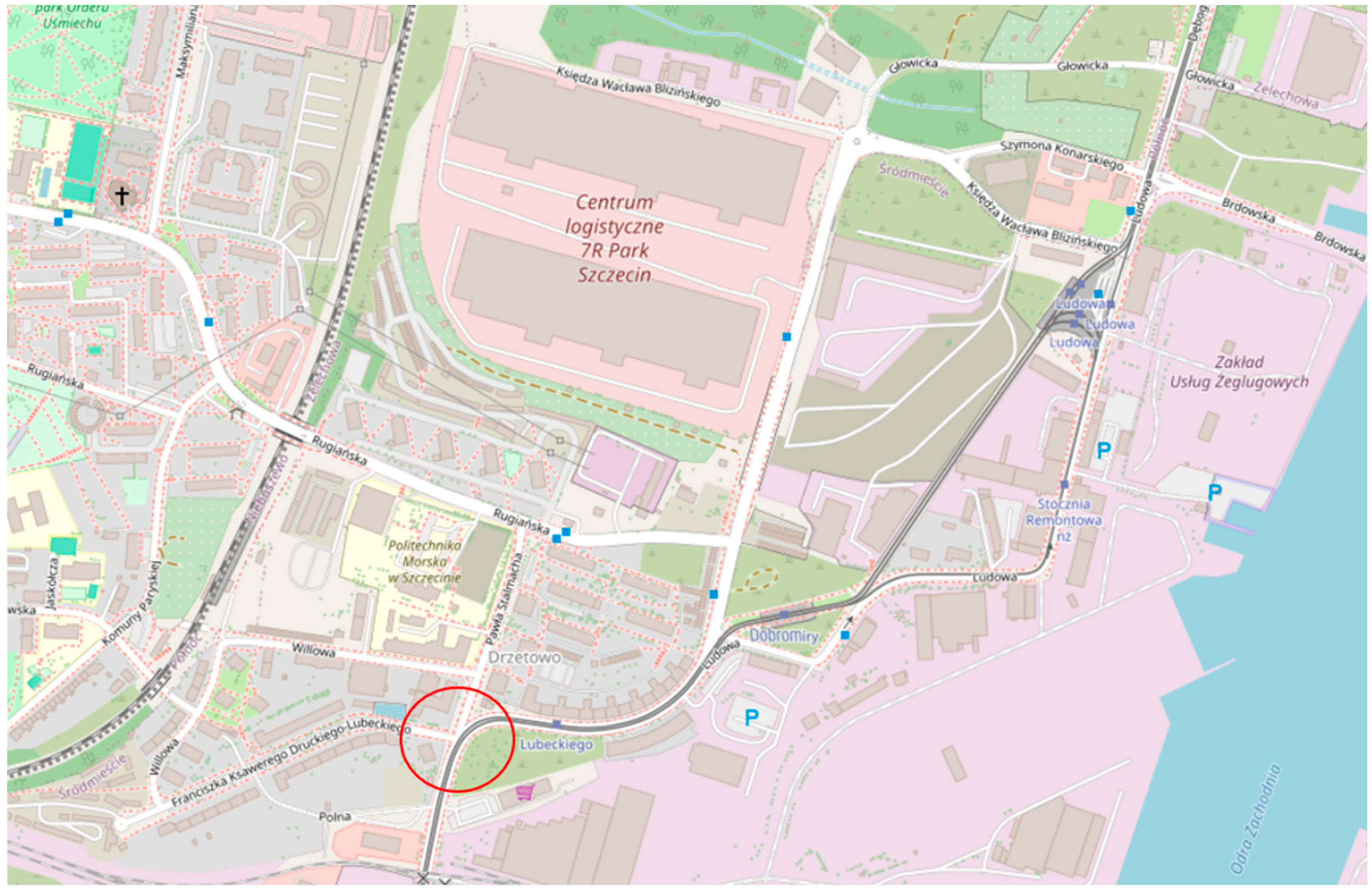
The traffic congestion analysis was conducted using the example of the intersection of Pawła Stalmacha Street and Ksawerego Lubeckiego-Druckiego Street in Szczecin (Figure 1). The intersection is located in the Drzetowo-Grabowo district and serves as a key transportation node in the northern part of the city. It connects traffic from the city center with industrial areas as well as the Oder Riverfront zones.

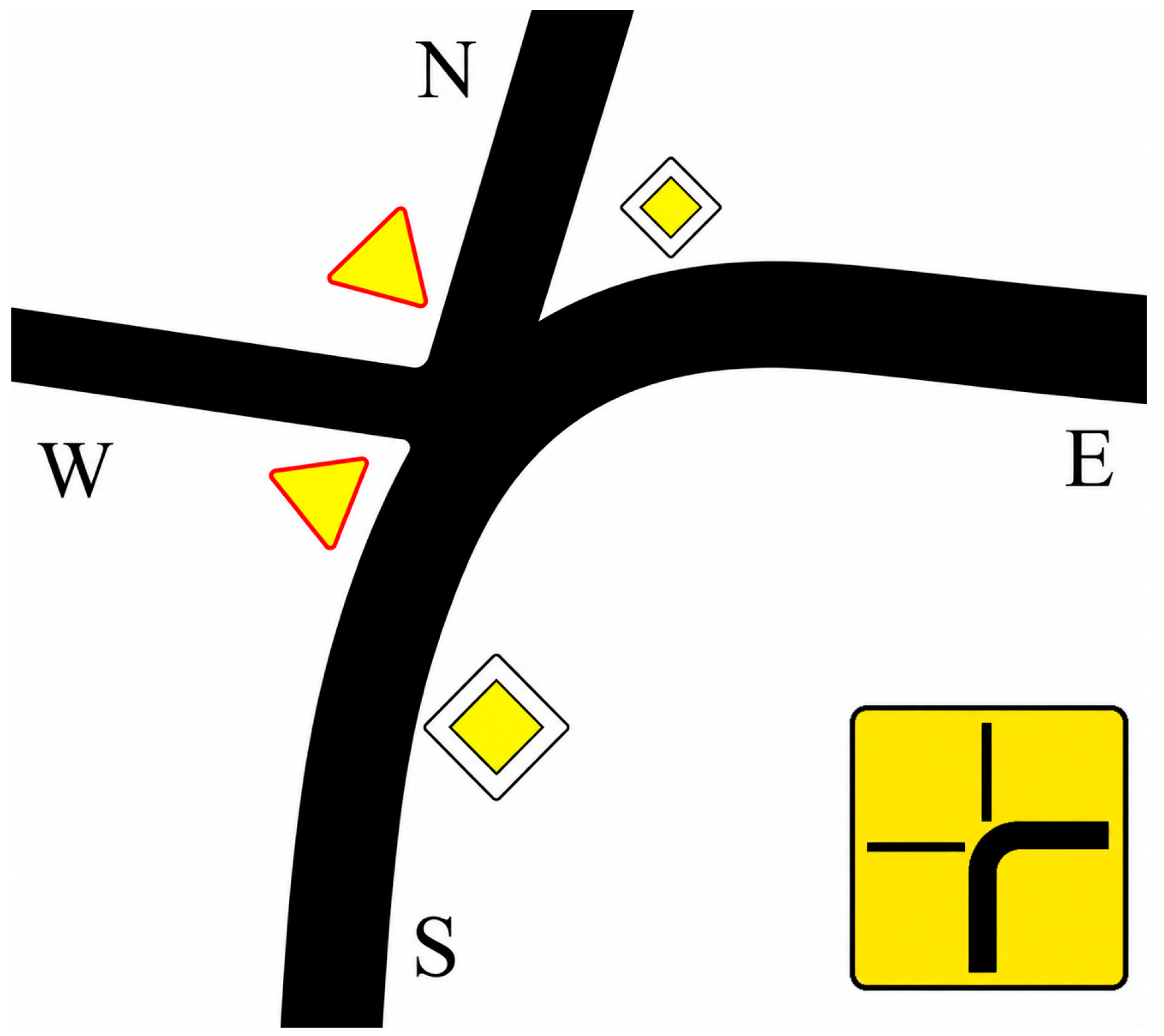
The intersection does not follow a conventional four-leg configuration but features an atypical, multileg, and asymmetric layout (Figure 2). Ksawerego Lubeckiego-Druckiego Street runs diagonally from the southwest to the northeast along a curved alignment. Pawła Stalmacha Street extends from south to north, forming an acute-angle intersection with the northeastern branch of Ksawerego Lubeckiego-Druckiego Street. The main traffic artery consists of the southern segment of Pawła Stalmacha Street together with the northeastern segment of Ksawerego Lubeckiego-Druckiego Street. These streets merge along a curve and are designated as priority roads (shown in gray), while the remaining approaches are secondary roads (shown in white).

An active tram track, integrated within the roadway, runs along the central axis of the main road, allowing trams to share the lane with vehicular traffic. The intersection is not signalized but is equipped with both vertical and horizontal traffic signage. A pedestrian crossing is located within the intersection area, in close proximity to the junction’s crown.

Figure 2. Plan of the intersection of Pawła Stalmacha Street–Ksawerego Druckiego-Lubeckiego Street. Source: own elaboration based on Figure 1.

Figure 2. Plan of the intersection of Pawła Stalmacha Street–Ksawerego Druckiego-Lubeckiego Street. Source: own elaboration based on Figure 1.

The intersection is located near residential neighborhoods, a large-format retail store, industrial areas, a shipyard, and a logistics center, which results in a high volume of heavy-vehicle traffic, particularly during peak hours. The analyzed intersection connects the center of Szczecin with northern districts, including Gocław, and provides access toward Police (a municipality neighboring Szczecin) and surrounding industrial areas, while also accommodating international traffic toward Germany. Furthermore, it serves as a significant public transport transfer point. The intersection handles both local and through traffic.

Traffic volume was measured in the field using direct observation methods. The measurements were conducted with video recording, enabling precise capture of traffic at the selected observation point. The camera position was chosen to provide a full view of the intersection cross-section. Each measurement session lasted 15 min, and the results were extrapolated to obtain hourly traffic volumes. This approach is commonly applied in traffic studies, where short-term observations are used as proxies for peak-hour conditions, provided that measurements are carried out during periods of relatively stable demand. The selected observation windows corresponded to peak traffic periods with no major disturbances, which supports their representativeness for the analyzed conditions. In some studies, a 15 min [61] (or at least 15 min [62]) measurement interval is recommended, with the results proportionally extrapolated to an hourly basis. However, other studies have applied shorter measurement intervals [63]. The recordings were subsequently analyzed in the laboratory, where all vehicles passing through the intersection were counted. Each vehicle was assigned to its respective travel direction and classified according to vehicle type. The collected data were entered into a preprepared analytical matrix.

Traffic measurements were carried out in February 2026 during two time intervals: 7:35–7:50 (morning peak) and 16:00–16:15 (afternoon peak). The data were processed to analyze traffic structure in terms of travel directions and vehicle categories. Hourly traffic volumes were calculated, considering fraction coefficients for each movement separately—both for the intersection approaches and the subsequent travel directions.

To clearly designate travel routes, a letter convention corresponding to cardinal directions was adopted: N (north), E (east), S (south), W (west). Movements between intersection approaches and travel directions were described using a two-letter code, where the first letter represents the intersection approach and the second indicates the travel direction (L—left, S—straight, R—right).

To assess congestion levels, a simulation approach was applied, modeling the road layout and traffic volumes based on the video-recorded data. The simulation was conducted in the Eclipse SUMO (Simulation of Urban MObility) environment [64], utilizing Python 3.13 [65] to automate the simulation process, data analysis, and result visualization.

The road network model was developed in the SUMO environment using the NETEDIT tool, and the representation of Szczecin’s street layout was based on a map from OpenStreetMap [60].

The key simulation parameters are presented in

Table 3. Calibrated parameters of the traffic simulation model in SUMO.

Parameter	Tractor-trailer with a semi-trailer	Trucks * (straight)	Trucks with trailers	Buses	Others (passenger cars and light delivery vehicles)
accel (m/s2)	0.8	1	0.7	1	2.6
decel (m/s2)	4	4.5	4	4.5	4.5
sigma (-)	0.5	0.5	0.5	0.5	0.5
tau (s)	1.6	1.5	1.7	1.7	1.2
minGap (m)	2.5	2	3	3	1.5

Note: * Heavy vehicles for transporting construction materials dominated. Source: own elaboration.

. The simulation uses the Krauss algorithm [66,67] implemented in SUMO. The parameter values, including acceleration, deceleration, driver reaction time (tau), minimum gap (minGap), and stochasticity factor (sigma), were selected based on the literature [68,69,70] values and calibrated using field measurements. Where possible, parameters were adjusted to better reflect observed traffic conditions using available field measurements of traffic flow and travel times. The chosen configuration enables a realistic representation of traffic interactions at the analyzed intersection.

Based on the conducted simulation and vehicle classification, the energy consumption of individual vehicles was calculated according to the HBEFA 4.2 (Handbook Emission Factors for Road Transport) methodology [71]. The calculations were based on HBEFA coefficients, which take into account factors such as:

• road type,
• traffic volume,
• vehicle category,
• speed,
• driving behavior (acceleration, braking, and steady-speed driving).

HBEFA is based on experimental data regarding fuel consumption under various traffic conditions. SUMO subsequently aggregates these values for the analyzed context (intersection, route, or road network) to calculate the total energy consumption of each vehicle. The comprehensive study, which included estimating total vehicle energy consumption based on the aforementioned factors, constructing appropriate road network models while accounting for traffic structure (by vehicle type), and performing validation, was conducted over two weeks (from 1 to 15 March 2026). Subsequent research stages took an additional two weeks.

The research approach is based on coupling microscopic traffic simulation in the SUMO environment with HBEFA 4.2 emission modeling at the individual vehicle level. Subsequently, for the purpose of analyzing system-level structure, the results were aggregated and subjected to econometric modeling. This approach enables a transition from the micro-level traffic dynamics to the macroscopic characterization of energy consumption within the transportation system.

In the subsequent stage of the analysis, the microsimulation outputs were aggregated and structured for econometric modeling. For each vehicle traversal through the analyzed intersection, a set of variables describing traffic conditions was derived, including average speed or time loss defined as the deviation from free-flow conditions. In parallel, vehicle-specific fuel consumption was estimated based on the implementation of HBEFA 4.2 emission factors within the simulation environment. This integrated dataset enabled the examination of relationships between traffic parameters and energy consumption at the level of individual observations, while preserving representativeness at the system level.

To identify the key determinants of fuel consumption, a general linear model (GLM) was employed, with unit fuel consumption as the dependent variable and vehicle speed and vehicle type as explanatory variables. Due to the strong correlation between time and speed, the time loss variable was not included simultaneously with the speed variable in the model specification, in order to avoid multicollinearity and potential inflation of effect estimates. The model was estimated using sigma-restriction parameterization, ensuring consistent interpretation of categorical effects.

Statistical significance was assessed using F-tests, while effect sizes were evaluated based on partial eta-squared. Additionally, non-centrality parameters and observed statistical power were examined to assess the robustness and generalizability of the results. To facilitate an interpretable representation of model outcomes, estimated marginal means (profile plots) were used to analyze the direction and functional form of the relationships while controlling for other factors in the model.

In the next step, utility-based approximations were analyzed to capture the relationship between traffic conditions and fuel consumption across different vehicle categories. This approach enabled the identification of nonlinear mechanisms associated with changes in traffic states, particularly transitions between free-flow and congested regimes. It also allowed for a comparative assessment of relative energy intensity across vehicle classes under varying operational conditions.

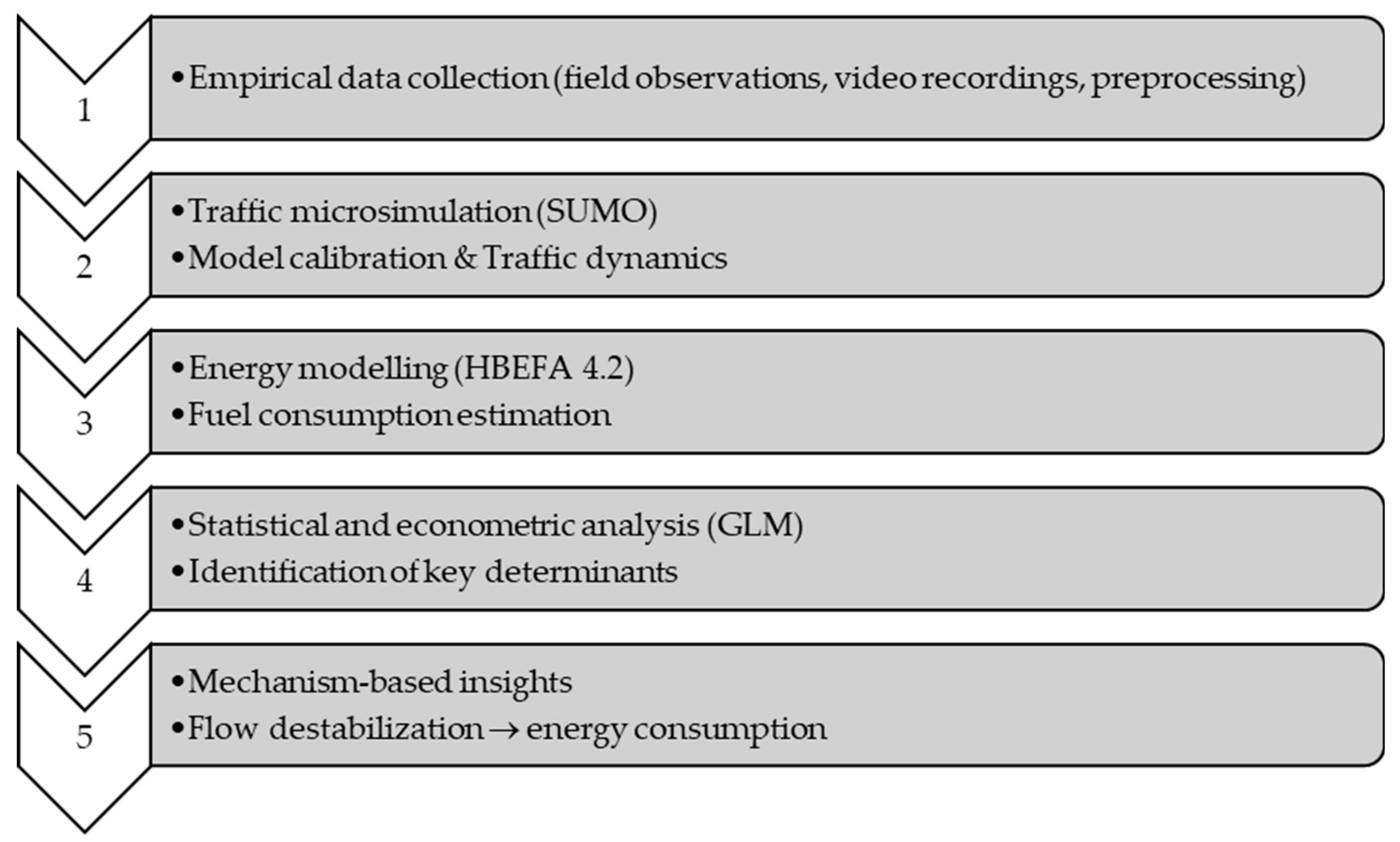
The research framework (Figure 3) conceptualized in this study is based on an integrated, multistage analytical structure linking empirical observation, traffic microsimulation, and energy modeling into a unified mechanism-oriented approach.

The framework consists of four sequential and interrelated layers:

• Empirical data acquisition layer (micro-level)—primary traffic data were collected through field observations using video recording under real-world peak-hour conditions. This stage ensures that the analysis is grounded in actual traffic behavior rather than synthetic or assumed inputs.
• Traffic microsimulation layer (meso-level)—the observed traffic structure was implemented in the SUMO environment, where vehicle interactions, speed dynamics, and flow instability were reproduced at a microscopic level. Model calibration was performed using empirical measurements to ensure consistency between simulated and real traffic conditions.
• Energy estimation layer (macro-level)—vehicle-level fuel consumption was estimated using the HBEFA 4.2 methodology, which translates dynamic driving patterns (speed, acceleration, stop–go cycles) into energy demand. This enables the direct linkage between traffic microdynamics and energy outcomes.
• Statistical and mechanism identification layer (macro-level)—the simulation outputs were aggregated and analyzed using a general linear model (GLM) to identify the relative contribution of key determinants, including vehicle speed and type. This stage allows the extraction of quantitative relationships and the identification of underlying mechanisms governing energy consumption.
• Mechanism-based insights (emergent level)—this stage integrates the statistically identified relationships into a mechanism-oriented representation of the system, focusing on interactions between traffic flow dynamics (e.g., speed variability, stop–go behavior) and energy consumption. The objective is to capture higher-order dependencies and formulate generalized patterns linking micro-level vehicle dynamics with macro-level energy outcomes.

Importantly, the framework is not purely simulation-based, but empirically anchored and mechanism-driven. Its primary objective is not only to estimate energy consumption levels, but to identify the structural processes through which traffic flow instability generates energy demand (emergent level). This integrated approach enables a transition from site-specific observations to generalizable insights at the level of transport system behavior.

The overall methodological framework was designed as an integrated approach combining empirical observations, traffic microsimulation, and statistical modeling within a unified analytical structure. This framework enables the simultaneous capture of micro-level driving dynamics and their macro-level implications for energy consumption within the transport system. As a result, it provides a comprehensive basis for evaluating the impact of traffic conditions and flow composition on energy demand at the level of an urban intersection.

4. Results

Traffic volume measurements conducted at the intersection of Pawła Stalmacha and Ksawerego Druckiego-Lubeckiego Streets in Szczecin provide critical data enabling a detailed analysis of vehicle flow characteristics, including its intensity, smoothness, and the operational efficiency of traffic organization in both temporal and directional dimensions. Based on these results, it is also possible to estimate the energy demand of transport in the study area using the advanced computational approach of HBEFA 4.2, representing a key component in assessing the environmental impact of the urban transport system.

Table 4. Traffic flow rate at the intersection of Pawła Stalmacha–Ksawerego Druckiego-Lubeckiego streets in Szczecin during the morning and afternoon peaks (veh/h) in February 2026.

Junction Entrance	Traffic Flow Rate (veh/h)
	Morning Peak	Afternoon Peak	Average
N	344	304	324
E	1004	588	796
S	728	1296	1012
W	68	40	54
Total	2144	2228	2186

Source: own study based on primary data obtained using the field method.

presents the traffic volumes at the approaches of the analyzed intersection during morning and afternoon peak periods.

Average vehicle flows across the junction approaches reveal pronounced spatial asymmetry in traffic distribution. The south (S) and east (E) approaches dominate the overall load, with 1012 and 796 veh/h, respectively, whereas the north (N) and west (W) approaches remain comparatively underutilized (324 and 54 veh/h). The total mean flow of 2186 veh/h indicates stability in overall junction demand despite marked heterogeneity among individual directions. This flow structure reflects an uneven allocation of traffic within the network, highlighting the primary corridors that drive junction movements and providing a critical reference point for system-level analysis and subsequent studies on junction dynamics. Importantly, the identified spatial asymmetry in traffic distribution is not unique to the analyzed location but reflects a broader structural characteristic of urban transport networks, where a limited number of dominant corridors disproportionately determine overall system performance.

For the purpose of this study, tram movements were excluded from the traffic analysis, as trams are classified within the track-based transport mode, distinct from road vehicle traffic.

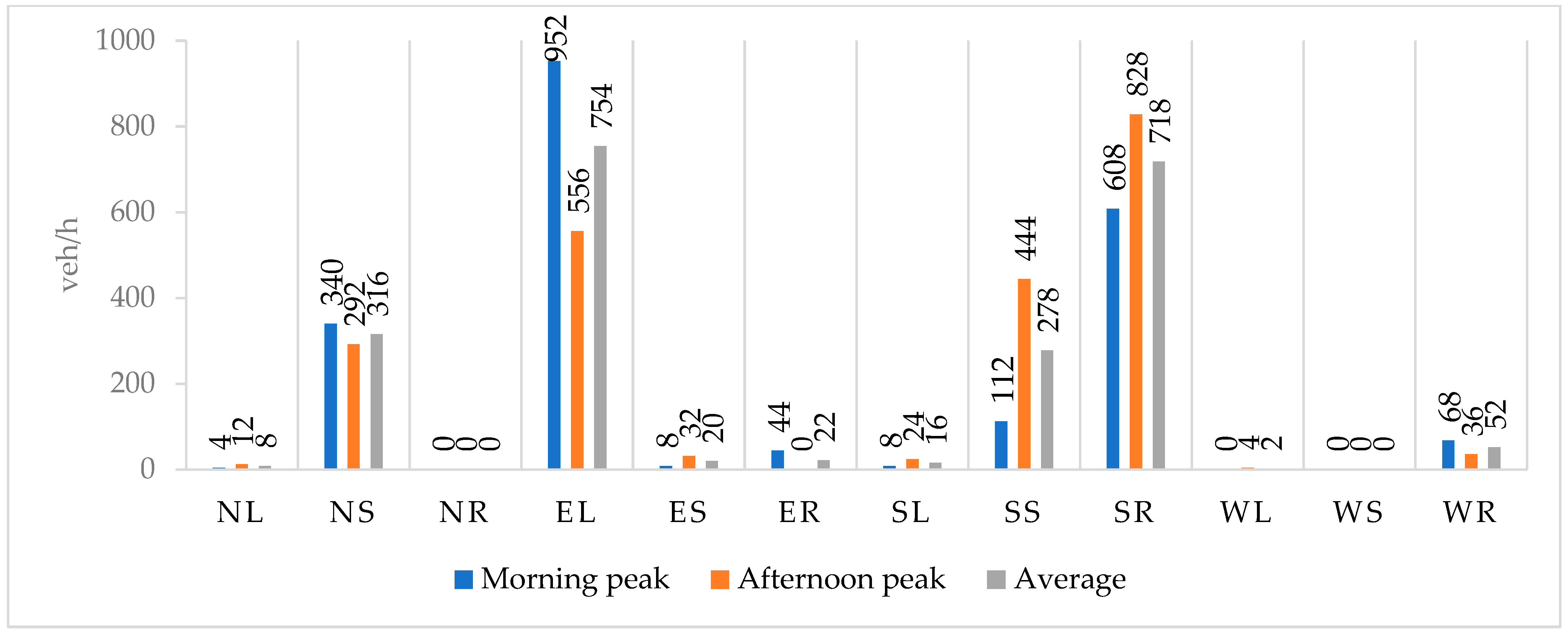
Figure 4 illustrates the variation in traffic volumes across individual turning movements at the study intersection for both peak periods and mean conditions. Movement labels follow an origin–destination convention, with the first letter indicating the approach direction and the second specifying the turning maneuver.

The observed traffic volumes at the study intersection exhibit pronounced spatiotemporal heterogeneity across both turning movements and peak periods, consistent with directional commuting dynamics and asymmetric demand profiles.

Overall, the highest volumes are concentrated along the east–west corridor, most notably for the EL (eastbound left-turn) movement. This movement attains a peak of 952 veh/h during the AM peak and sustains a high mean flow of 754 veh/h, indicating a dominant left-turn demand from the eastern approach. Such a pattern is likely associated with directional inbound commuting toward major employment centers, although this interpretation cannot be directly verified without a complementary survey. A marked reduction is observed in the PM peak (556 veh/h), underscoring a strong diurnal imbalance. A similarly critical movement is SR (southbound right-turn), which dominates during the PM peak (828 veh/h) and maintains a high average volume (718 veh/h). In contrast to EL, SR exhibits higher demand in the PM (608 veh/h in AM vs. 828 veh/h in PM), suggesting its role in outbound, home-based trip making. The elevated right-turn demand may further reflect lower operational impedance and favorable downstream network conditions. Movements from the northern approach are comparatively moderate and stable. The NS (northbound through) movement shows limited temporal variability (340 veh/h in AM and 292 veh/h in PM), yielding an average of 316 veh/h. This indicates a relatively balanced through-flow along the north–south axis, likely associated with background or distributed traffic rather than strongly directional commuting. Turning movements from this approach (NL, NR) are negligible or absent, potentially due to geometric design constraints or prohibited maneuvers. On the southern approach, the SS (southbound through) movement exhibits substantial temporal asymmetry, with low demand in the AM peak (112 veh/h) and a notable increase in the PM peak (444 veh/h). This pattern is indicative of directional return flows, likely toward residential areas located north of the intersection. All remaining movements (e.g., ES, ER, SL, WR) are characterized by low volumes, generally below 55 veh/h on average, and, therefore, contribute marginally to overall intersection performance. Several movements (e.g., NR, WS, and partially WL) are effectively inactive, suggesting either operational restrictions or negligible functional relevance within the network. From an operational standpoint, the concentration of demand in a limited number of critical movements—particularly EL and SR—implies a heightened risk of capacity constraints, queue spillback, and delay propagation. Without appropriate control strategies (e.g., protected signal phases or exclusive turn lanes), these dominant flows are likely to govern intersection performance.

Table 5. Empirical validation of a microscopic traffic simulation framework using multiclass boundary flow measurements.

Route		NL	NS	NR	N	EL	ES	ER	E	SL	SS	SR	S	WL	WS	WR	W	All
Tractor–trailer with a semi-trailer	SUMO [veh/h]	0	8	0	8	24	0	0	24	0	0	46	46	0	0	0	0	78
	Real [veh/h]	0	8	0	8	24	0	0	24	0	0	46	46	0	0	0	0	78
	Error [%]	-	0	-	0	0	-	-	0	-	-	0	0	-	-	-	-	0
Trucks * (straight)	SUMO [veh/h]	0	10	0	10	14	0	0	14	0	10	30	40	0	0	0	0	64
	Real [veh/h]	0	10	0	10	14	0	0	14	0	10	30	40	0	0	0	0	64
	Error [%]	-	0	-	0	0	-	-	0	-	0	0	0	-	-	-	-	0
Trucks with trailers	SUMO [veh/h]	0	0	0	0	4	0	0	4	0	0	6	6	0	0	0	0	10
	Real [veh/h]	0	0	0	0	4	0	0	4	0	0	6	6	0	0	0	0	10
	Error [%]	-	-	-	-	0	-	-	0	-	-	0	0	-	-	-	-	0
Buses	SUMO [veh/h]	0	0	0	0	2	0	0	2	0	0	2	2	0	0	0	0	4
	Real [veh/h]	0	0	0	0	2	0	0	2	0	0	2	2	0	0	0	0	4
	Error [%]	-	-	-	-	0	-	-	0	-	-	0	0	-	-	-	-	0
Others (passenger cars and light delivery vehicles)	SUMO [veh/h]	8	298	0	306	711	20	23	754	16	268	634	918	2	0	52	54	2032
	Real [veh/h]	8	298	0	306	710	20	22	752	16	268	634	918	2	0	52	54	2030
	Error [%]	0	0	-	0	0.14	0	4.35	0.27	0	0	0	0	0	-	0	0	0.1
All	SUMO [veh/h]	8	316	0	324	755	20	23	798	16	278	718	1012	2	0	52	54	2188
	Real [veh/h]	8	316	0	324	754	20	22	796	16	278	718	1012	2	0	52	54	2186
	Error [%]	0	0	-	0	0.13	0	4.35	0.25	0	0	0	0	0	-	0	0	0.09

Note: “-” denotes that the relative error is undefined in this case, as the reference value equals zero, resulting in division by zero in the percentage error formula. * Heavy vehicles for transporting construction materials dominated. Source: own study based on primary field data and simulation modeling.

presents the empirical validation of the microscopic traffic simulation framework using multiclass boundary flow measurements. The results compare simulated traffic volumes obtained from SUMO with field observations across different vehicle classes and movement directions. The analysis covers all major vehicle categories and demonstrates the level of agreement between simulation outputs and real-world data.

The results from Table 5 indicate perfect agreement for heavy vehicle categories, including tractor–trailers with semi-trailers, straight trucks, trucks with trailers, and buses, where the relative error is 0%. For passenger cars and light delivery vehicles, the relative error remains very low, reaching 0.10% at the total class level. At the directional aggregation level within this class, small deviations are observed, with the highest error equal to 4.35% for a single movement component, while most other movements exhibit errors below 0.3%. The total traffic volume shows a relative error of only 0.09%, confirming a very high level of agreement between simulated and empirical data.

The intersection operates under a highly unbalanced demand structure, with dominant, time-dependent turning flows shaping its performance. These findings provide a robust empirical basis for subsequent capacity analysis and advanced traffic modeling, including microsimulation-based evaluation of control strategies.

The morning peak (

Table 6. Road traffic structure during the morning traffic rush (%).

Junction entrance	Tractor–trailer with a semi-trailer	Trucks * (straight)	Trucks with trailers	Buses	Others (passenger cars and light delivery vehicles)	Total
N	3.49	2.32	0.00	0.00	94.19	100.00
E	4.78	2.79	0.80	0.40	91.23	100.00
S	9.34	9.89	1.10	0.55	79.12	100.00
W	0.00	0.00	0.00	0.00	100.00	100.00
Total	5.97	5.04	0.75	0.37	87.87	100.00

Note: * Heavy vehicles for transporting construction materials dominated. Source: own study based on primary data obtained using the field method.

) is characterized by a relatively high share of heavy vehicles, with a total contribution of approximately 11.76% when aggregating tractor–trailers, straight trucks, and trucks with trailers. This elevated presence is particularly pronounced on the southern approach, where heavy vehicles account for over 20% of the traffic stream (9.34% tractor–trailers with a semi-trailer and 9.89% straight trucks), indicating a strong influence of freight-related movements, likely associated with logistics and freight forwarding activity as noted. The eastern approach also exhibits a moderate share of heavy vehicles (approximately 8.37% combined), while the northern approach shows a lower, but still notable, contribution (5.81%). In contrast, the western approach is composed exclusively of passenger cars and light-duty vehicles, suggesting either functional differences in network connectivity or restrictions affecting heavy vehicle access. Bus shares remain marginal across all approaches, not exceeding 0.55%, indicating limited public transport penetration in the observed traffic stream. From an energy perspective, this elevated share of heavy vehicles in the morning peak is particularly critical, as heavy-duty vehicles exhibit disproportionately higher fuel consumption rates under stop-and-go conditions, thereby amplifying the overall energy intensity of traffic flow during this period.

In the afternoon peak (

Table 7. Road traffic structure during the afternoon traffic rush (%).

Junction entrance	Tractor–trailer with a semi-trailer	Trucks * (straight)	Trucks with trailers	Buses	Others (passenger cars and light delivery vehicles)	Total
N	1.31	3.95	0.00	0.00	94.74	100.00
E	0.00	0.00	0.00	0.00	100.00	100.00
S	1.85	0.62	0.31	0.00	97.22	100.00
W	0.00	0.00	0.00	0.00	100.00	100.00
Total	1.26	0.90	0.18	0.00	97.66	100.00

Note: * Heavy vehicles for transporting construction materials dominated. Source: own study based on primary data obtained using the field method.

), the traffic structure shifts markedly toward a dominance of light vehicles, with the “others” category accounting for 97.66% of total flow. The share of heavy vehicles decreases substantially to approximately 2.34% overall, reflecting a significant reduction in freight activity during this period. This decline is evident across all approaches, most notably on the southern approach, where the combined heavy vehicle share drops from over 20% in the morning to below 3%. Similarly, the eastern and western approaches become entirely dominated by passenger cars and light delivery vehicles (100%), indicating a near absence of heavy vehicle movements. The northern approach retains a small share of straight trucks (3.95%), suggesting residual freight activity, but at a much lower intensity than in the morning peak. Notably, buses are absent in the afternoon dataset, further emphasizing the private and light-duty character of traffic during this period. This structural shift toward light-duty vehicles implies not only a reduction in total fuel consumption but also a change in the sensitivity of the system to congestion, as passenger vehicles exhibit lower marginal fuel penalties under disrupted flow conditions compared to heavy-duty vehicles.

Overall, the results indicate a strong temporal differentiation in traffic composition, with freight traffic concentrated in the morning peak and largely dissipating in the afternoon. This pattern is consistent with logistics and freight forwarding supply schedules and has important implications for capacity analysis, pavement wear, and intersection control strategies, as heavy vehicles disproportionately affect both operational performance and infrastructure degradation.

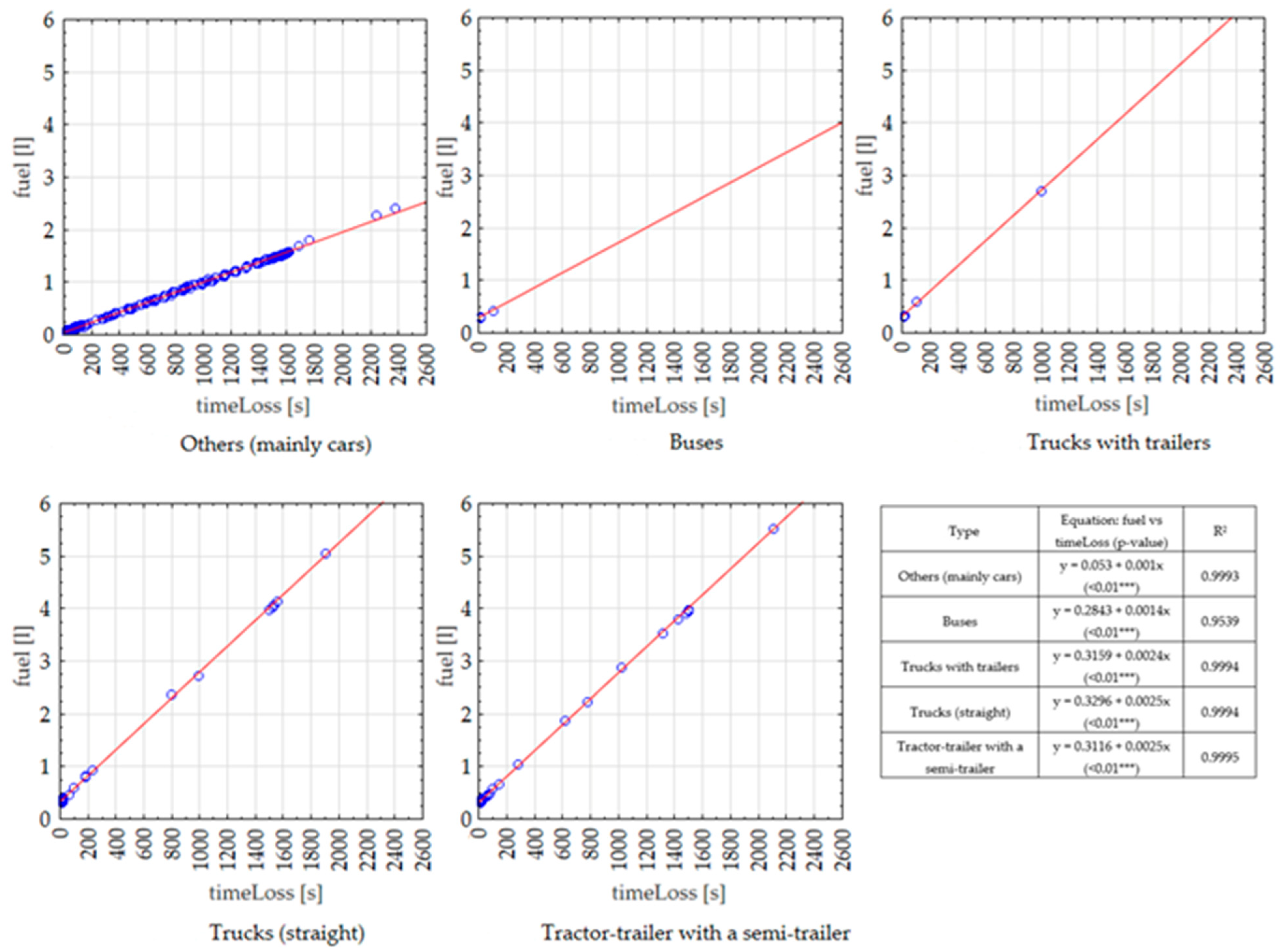
Fuel consumption estimated using SUMO with HBEFA 4.2 shows a near-linear relationship with travel time loss under congested traffic conditions, suggesting that delay is a strong proxy for energy intensity in stop-and-go traffic (Figure 5).

An important feature visible in Figure 5 is the consistency of the linear relationship across all vehicle categories, combined with clear differences in slope magnitude. This indicates that time loss acts as a universal driver of fuel consumption, while the sensitivity to this factor is vehicle-specific. In particular, heavier vehicle categories exhibit steeper gradients, suggesting that congestion-related delays translate into disproportionately higher energy penalties for these vehicles. This confirms that the impact of traffic disruption is not uniform, but systematically amplified by vehicle characteristics.

The empirical relationship between time loss and fuel consumption exhibits a strongly monotonic and near-deterministic pattern, indicating that disruptions to traffic flow constitute a primary driver of transport energy intensity. The consistency of this relationship across vehicle classes suggests that congestion-induced delay should not be viewed solely as a degradation of travel conditions, but, rather, as a direct carrier of energy and, by extension, environmental costs. This finding suggests that travel time delay may serve as an effective proxy variable in large-scale energy and emission modeling, particularly in data-constrained environments where direct fuel measurements are not available.

As shown in Figure 5, each second of time loss—defined as the difference between actual travel time under congested conditions and free-flow travel time—translates into a systematic increase in fuel consumption. The effect amounts to approximately 1 mL/s for other vehicles (primarily passenger cars and light commercial vehicles), 1.4 mL/s for buses, and 2.4–2.5 mL/s for heavy-duty vehicles.

When scaled to one hour of cumulative delay, this corresponds to an additional fuel consumption of approximately 3.6 L for passenger cars and light commercial vehicles, 5.04 L for buses, and 8.64–9 L for heavy-duty vehicles. These findings highlight the heterogeneous energy cost intensity of congestion, with heavy-duty vehicles exhibiting a disproportionately higher sensitivity to disruptions in traffic flow.

From an analytical perspective, not only does time loss under congestion conditions affect fuel consumption, but vehicle speed (as an indicator of prevailing traffic conditions) and vehicle type also play a significant role. Travel time is strongly correlated with speed. Therefore, it was not included simultaneously in the subsequent model specification to avoid multicollinearity and potential inflation of estimated effects (see

Table 8. Univariate test of significance of effects (parameterization with sigma-restrictions).

Effect	SS	Degree of freedom	MS	F	p	Partial eta-square	Non-centrality	Observed power (alpha = 0.05)
intercept	112.4801	1	112.4801	1498.757	<0.001	0.4071	1498.7570	~1.00
speed	249.5374	1	249.5374	3324.997	<0.001	0.6037	3324.9970	~1.00
type	35.8534	4	8.9633	119.433	<0.001	0.1795	477.7330	~1.00
error	163.8318	2180	0.0750

Note: y = fuel consumption (L). Source: own study based on primary field data and simulation modeling.

).

The analysis revealed a statistically significant effect of both vehicle speed and vehicle type on fuel consumption. Speed emerged as the strongest predictor (η²p = 0.60), accounting for the majority of the variance in fuel use. Vehicle type was also statistically significant (η²p = 0.18), although its effect was considerably weaker in comparison. The non-centrality parameters further indicated that the effect associated with speed was substantially stronger than that of vehicle type. The model exhibited very high statistical power (approximately 1.00). The residual mean square error (MS error = 0.075) reflects unexplained variability in fuel consumption and was low, indicating a good overall model fit. From a transport systems perspective, this result underscores the dominant role of traffic flow conditions over fleet composition in determining real-world fuel consumption, suggesting that operational interventions targeting speed stabilization may yield greater energy savings than structural changes in vehicle mix alone (for example, by introducing traffic restriction signs for vehicles with a GVM (gross vehicle mass) above a specified limit).

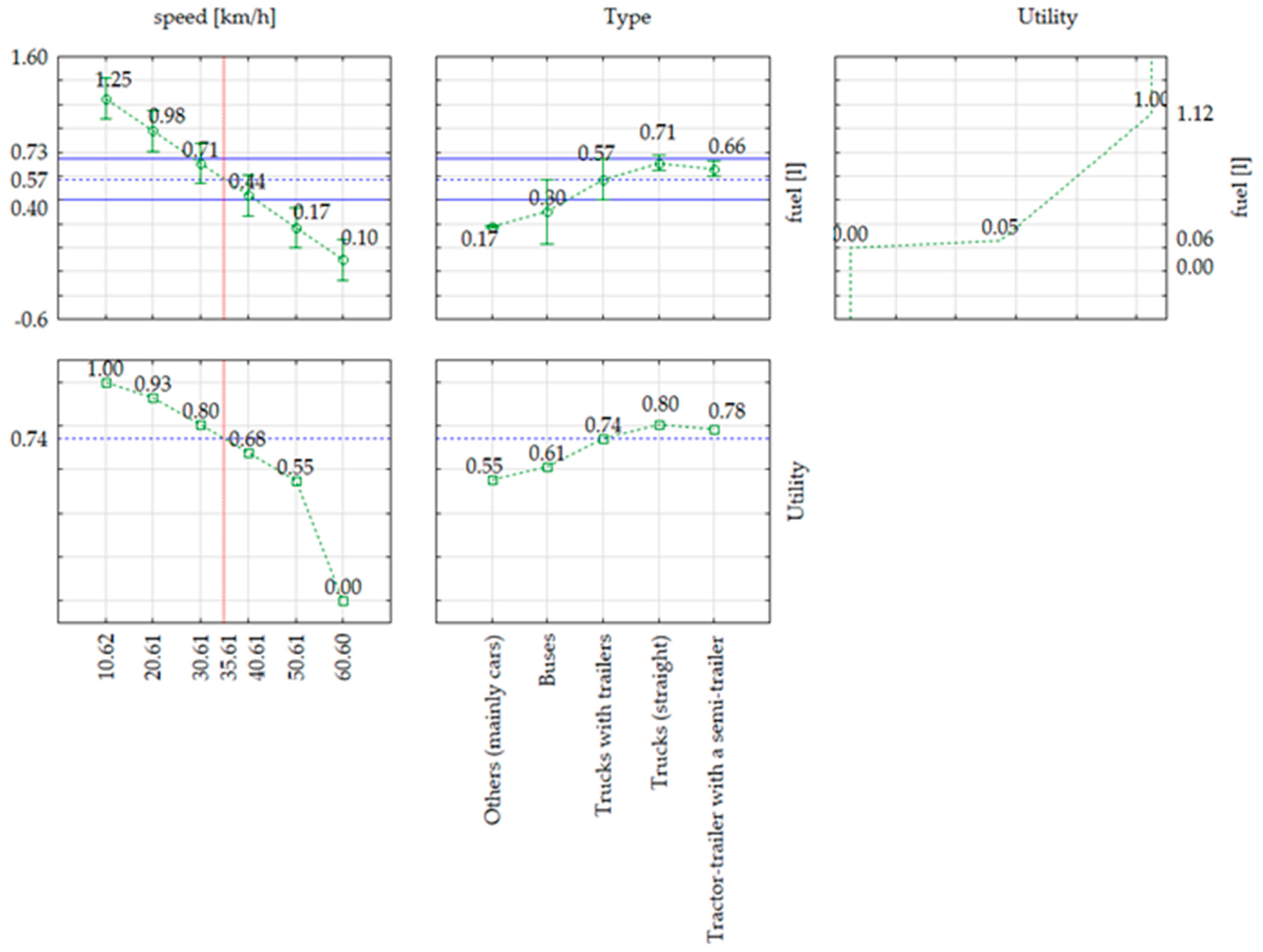
To complement the inferential results of the GLM (general linear model), estimated marginal means (profile plots) were employed to provide an interpretable representation of adjusted effects of vehicle speed and vehicle type on fuel consumption. Unlike significance testing, which identifies whether effects are statistically detectable, profile-based visualization allows for direct assessment of the functional form, direction, and relative magnitude of effects under model-adjusted conditions.

The profiles for vehicle speed indicate a clear and systematic relationship with fuel consumption, suggesting a strong monotonic effect whereby increases in speed are associated with substantial changes in fuel use. This pattern is consistent with the large effect size identified in the GLM results (η²p = 0.60), confirming that speed constitutes the dominant explanatory factor in the model. Importantly, the profile structure provides additional substantive insight beyond the ANOVA decomposition, as it allows the identification of how fuel consumption behaves across the observed speed range rather than only quantifying overall variance explained.

In the case of vehicle type, the profile plots reveal distinct but comparatively more moderate separations between categories, indicating heterogeneity in fuel consumption across vehicle classes. Although statistically significant, these differences are less pronounced than those associated with speed (η²p = 0.18), suggesting that vehicle configuration contributes to baseline variability in fuel consumption rather than driving its primary dynamics. The adjusted means further highlight that the effect of vehicle type is relatively stable across the range of speeds, with no evidence of strong divergence in profile shapes between categories.

Overall, the profile-based analysis reinforces the conclusions drawn from the GLM tests, while providing a more behaviorally interpretable depiction of model outputs. In particular, the results suggest that fuel consumption is primarily governed by dynamic driving conditions, proxied by speed, whereas vehicle type acts as a secondary structural determinant shaping baseline consumption levels. This distinction is critical from a transportation systems perspective, as it separates operational (speed-related) from structural (vehicle-related) sources of variability in energy demand.

Figure 6 provides further insight into the structure of the system by illustrating the combined effect of speed and vehicle type on fuel consumption through a utility-based representation. A key observation is the nonlinear response of the system to decreasing speed. While initial reductions in speed result in moderate changes, a threshold-like behavior becomes visible beyond a certain point (indicated by the vertical reference line), where fuel consumption increases more rapidly. This suggests that traffic systems operate in two distinct regimes: a relatively stable regime with gradual changes, and an unstable regime where small additional disturbances lead to disproportionately higher energy demand. This transition indicates that congestion should not be interpreted as a continuous process, but, rather, as a regime shift driven by flow destabilization. Additionally, the monotonic increase in utility across vehicle categories confirms that heavier vehicles systematically contribute more to overall energy demand, reinforcing their role as amplifiers of congestion effects under deteriorating traffic conditions.

The analysis of approximated utility profiles reveals a distinctly heterogeneous structure of fuel consumption burdens driven by traffic conditions and vehicle class composition. In particular, a pronounced nonlinear relationship emerges between traffic operating conditions and unit fuel consumption, indicating a strong sensitivity of the transport system to variations in traffic flow dynamics.

With respect to traffic speed, a clear monotonic decline in fuel consumption levels is observed as average speed increases. The highest fuel burdens occur under low-speed regimes, typically associated with congested or disrupted traffic states, where frequent stopping events and high-intensity acceleration phases dominate the driving cycle. As speed increases, traffic flow becomes progressively more stable, resulting in a systematic reduction in unit fuel consumption.

A pronounced hierarchical structure is evident across vehicle categories. The highest fuel consumption levels are observed for trucks (straight) (approx. 0.71 L), representing heavy rigid freight vehicles predominantly engaged in construction material and bulk freight transport. A slightly lower yet still substantially elevated level is identified for tractor–trailer with a semi-trailer (approx. 0.66 L), reflecting articulated heavy-duty vehicle combinations characterized by high inertial resistance and substantial stop-and-go energy losses in urban traffic conditions.

The next tier is formed by trucks with trailers (approx. 0.57 L), which exhibit moderately high fuel demand driven by both increased gross vehicle mass and constrained operational dynamics under interrupted traffic regimes. Buses (approx. 0.30 L) constitute an intermediate category, where higher vehicle mass is partially offset by comparatively more stable operational patterns and more regular service cycles.

The lowest fuel consumption levels are consistently observed for other vehicles (approx. 0.17 L), encompassing mainly passenger cars and light-duty delivery vehicles. This category provides a clear benchmark for comparison, reflecting substantially lower fuel intensity under urban driving conditions. The results highlight that both fleet composition and traffic flow stability exert dominant and strongly differentiated effects on unit fuel consumption. These effects are inherently nonlinear, underscoring the critical role of traffic composition and operational conditions in determining fuel demand within urban transport systems. Moreover, the structure of road traffic flow exhibits a strongly nonlinear mechanism governing fuel-related energy consumption, where the decisive factor is not the average speed level itself, but, rather, its distribution shaped by the dynamic reconfiguration of vehicular streams. The estimated utility approximations indicate the presence of distinct operational regimes of the transport system, in which transitions between smooth-flow and disturbed states induce a qualitative shift in fuel consumption patterns that extends beyond linear traffic volume effects. In this framework, congestion should be interpreted as a dynamic process of traffic flow destabilization that systematically increases fuel consumption through intensified speed fluctuations and repeated acceleration cycles.

The near-perfect linearity observed across all vehicle categories indicates that congestion-related energy losses scale proportionally with time loss, while the variation in slope reflects a systematic differentiation in sensitivity across vehicle types. This transition reflects a change in system behavior, where the relationship between traffic conditions and fuel consumption shifts from approximately linear to strongly nonlinear. Importantly, the combined interpretation of both figures indicates that the effect of time loss is not independent of traffic conditions, but is significantly amplified under unstable flow regimes. The consistency of these patterns across vehicle categories suggests that they reflect structural properties of traffic systems rather than scenario-specific effects.

Overall, the results indicate that urban transport energy demand is primarily governed by the structure of traffic flows and operational conditions, with speed variability and traffic composition across lanes and approaches playing a dominant role in shaping fuel consumption patterns.

Importantly, the observed relationships are not specific to the analyzed intersection but reflect a broader structural mechanism linking traffic flow destabilization to energy consumption. The consistency of the identified patterns across vehicle types and traffic conditions suggests that the results can be interpreted as representative of a wider class of urban traffic systems, particularly those characterized by asymmetric demand structures and frequent flow disruptions.

5. Discussion

5.1. Academic Polemic

Beyond confirming existing empirical findings, this study contributes to the conceptualization of congestion as a mechanism of traffic flow destabilization, which directly translates into increased energy consumption. This perspective extends the current literature by shifting the focus from static descriptors of traffic conditions (e.g., average speed or volume) toward dynamic system properties governing energy demand.

The concept of traffic flow destabilization differs fundamentally from traditional congestion measures such as delay or level of service (LOS) in that it captures dynamic variations in traffic conditions rather than average performance levels. Conventional metrics describe congestion using aggregated indicators (e.g., mean speed or delay), implicitly assuming relatively stable traffic states. In contrast, traffic flow destabilization reflects temporal fluctuations in vehicle behavior, such as speed variability and irregular acceleration patterns. This distinction is important because traffic scenarios with similar average speeds or delays may exhibit substantially different levels of instability, resulting in different fuel consumption outcomes. Therefore, destabilization provides a more behaviorally relevant measure, directly linked to energy use. The practical implication is that improving transport energy efficiency should focus not only on reducing average delay, but also on limiting traffic flow variability. This shifts the emphasis of traffic management toward strategies that enhance flow stability, as even moderate fluctuations can significantly increase fuel consumption.

The results of this study confirm that traffic flow conditions, particularly speed and congestion, constitute the primary determinants of fuel consumption in urban transport systems. This finding is consistent with recent research emphasizing the dominant role of traffic dynamics over static vehicle characteristics. In another study, empirical analyses show that traffic conditions, such as speed variability and flow instability, significantly influence fuel consumption and emissions in real-world urban driving conditions [49]. These findings directly confirm the strong effect of speed identified in our study (η²p = 0.60), confirming that speed acts as an integrated indicator of congestion and vehicle fuel consumption.

The near-linear relationship observed between time loss and fuel consumption further aligns with recent studies highlighting the critical role of congestion-induced operating conditions. In particular, vehicle idling and stop-and-go dynamics have been shown to substantially increase fuel consumption due to low engine efficiency under such conditions [72]. This supports the interpretation that delay is not merely a temporal inefficiency but a direct proxy for energy intensity. Similarly, recent intersection-based studies indicate that frequent stopping significantly increases fuel consumption in urban networks [73]. In this context, the present study contributes by demonstrating a highly regular and near-deterministic relationship between delay and fuel consumption, suggesting that travel time loss can be operationalized as a robust surrogate variable in fuel-intensity modeling. This is particularly relevant in large-scale applications where direct fuel measurements remain unavailable.

The relatively weaker, although still statistically significant, effect of vehicle type (η²p = 0.18) is also consistent with recent findings. While vehicle technology and configuration influence absolute fuel consumption levels, their impact is strongly moderated by traffic conditions and operational context. For instance, recent simulation-based research shows that fuel consumption varies significantly across vehicle types depending on congestion intensity and driving cycles, with stop-and-go traffic amplifying differences between vehicle categories [74].

The profile-based analysis further reveals a nonlinear structure of fuel consumption across traffic regimes, particularly under low-speed conditions. This is consistent with recent work in traffic flow theory and energy modeling, which demonstrates that unstable traffic states characterized by speed fluctuations and frequent accelerations lead to disproportionately high fuel consumption [49]. In this sense, the findings support a growing consensus that average speed alone is insufficient to explain energy use, and that variability and flow disruptions (profiles) must be explicitly considered.

From a network perspective, the pronounced spatial asymmetry observed at the analyzed intersection reflects broader structural patterns in urban transport systems. Recent studies highlight that traffic congestion and associated energy costs are highly unevenly distributed across networks, with critical nodes and corridors disproportionately shaping system performance [75,76,77]. The identification of dominant turning movements in the present study (e.g., EL and SR) is, therefore, consistent with this literature, confirming that localized bottlenecks play a central role in determining both operational efficiency and energy consumption.

Overall, the findings reinforce a key paradigm emerging in recent transportation research: urban transport energy demand is primarily governed by dynamic traffic conditions rather than static system attributes. In this framework, congestion should be understood not only as a loss of time but as a systemic process of traffic flow destabilization that directly translates into increased energy consumption. This perspective highlights the need for integrated approaches combining traffic flow theory, energy modeling, and traffic management strategies in order to effectively mitigate the environmental impact of urban transport systems.

The transferability of the identified mechanism is supported by the geometric and functional characteristics of the analyzed intersection. The junction is multileg and asymmetric, with a complex priority structure, which generates inherent flow disturbances at merging points. In combination with mixed traffic operation and the absence of signal control, this leads to frequent priority conflicts and variability in vehicle trajectories. These features are characteristic of many urban intersections, particularly those located at the interface between residential, industrial, and arterial corridors. While specific geometric parameters (e.g., turning radii or lane widths) may vary across locations, the key factors influencing traffic flow, namely interaction intensity, merging and diverging movements, and constrained maneuvering space, remain comparable. Therefore, the identified relationship between traffic flow instability and fuel consumption can be considered representative of a broader class of complex urban nodes.

5.2. Limitations

It should be emphasized that the presented research approach is based on the analysis of a single road intersection, which formally limits the direct generalizability of the results to entire transportation networks. However, the intersection under study features a high degree of geometric complexity, traffic flow asymmetry, and the presence of heavy vehicles, making it a representative case for many real-world urban layouts. Consequently, the results should be interpreted as generalizable in terms of underlying mechanisms rather than specific numerical values.

The use of microsimulation within the Eclipse SUMO environment, coupled with the HBEFA 4.2 model, relies on certain modeling assumptions, particularly regarding driver behavior and vehicle characteristics. Nonetheless, this approach represents the current standard in analyses of transportation fuel energy consumption and enables the capture of relationships that are not directly observable in field conditions. Importantly, integrating primary empirical data collected in the field with the simulation helps mitigate errors arising from the purely model-based nature of the analysis.

Another limitation lies in the use of data from only two time periods (morning and afternoon peak hours). This selection allows the study to capture contrasting states of the transportation system, but does not reflect the full diurnal variability. At the same time, it enables a focus on the most critical traffic conditions, which have the greatest influence on energy consumption and are particularly relevant for decision-makers and traffic management strategies.

It should be noted that the use of 15 min observation intervals represents a limitation of the study. The extrapolation of short-term measurements to hourly values assumes relatively stable traffic conditions within the analyzed period, which may not fully capture temporal fluctuations occurring over the entire peak hour. Although the measurements were conducted during periods of high and relatively consistent traffic demand, some variability may not be reflected in the extrapolated values. Therefore, the results should be interpreted as representative of typical peak conditions rather than exact hourly totals.

In the statistical modeling, time loss and speed were intentionally not included simultaneously due to their high interdependence. This choice does not constitute a limitation but a deliberate simplification of the model, allowing for stable and interpretable effect estimates. As a result, the analysis focuses on speed as a synthetic variable, integrating the influence of multiple aspects of traffic conditions.

6. Conclusions

The results provide strong empirical support for the proposed hypothesis, demonstrating that fuel consumption in urban transport systems is primarily driven by traffic flow destabilization rather than by traffic volume alone or fleet composition. This finding establishes a mechanism-based interpretation of transport energy demand, in which congestion is understood as a dynamic process generating energy-intensive speed fluctuations and stop-and-go cycles.

The findings further indicate that the geometric and organizational characteristics of the analyzed intersection induce forced speed reductions and stops, which directly increase fuel consumption through more frequent and intensive acceleration cycles. Thus, the main objective of the study, linking traffic microdynamics with the macroscopic characteristics of energy consumption, has been achieved. The specific objective has also been fulfilled, as it was demonstrated that variability in traffic conditions, rather than their average level, is of primary importance.

The novelty of this study lies in demonstrating that transportation energy consumption can be interpreted as an emergent outcome resulting from traffic flow destabilization, rather than merely as a function of macroscopic parameters. In particular, it is shown that the microstructure of the road network, including its geometry and traffic organization, can generate disproportionately high fuel consumption (and associated energy costs) that are not captured by classical models based on average speed or traffic volume, but, rather, on the full speed profiles. By combining microsimulation, emission modeling, and econometric analysis, the study provides an empirically validated, mechanism-based explanation of the relationship between congestion and energy consumption. The results obtained from the statistical analysis show a coherent mechanism-oriented representation of the system. Rather than focusing on individual variables or isolated relationships, the procedure aims to identify consistent patterns of interaction between traffic flow characteristics and energy consumption. The analysis involves the structured interpretation of statistically significant relationships (identified in the GLM) in the context of traffic flow theory, with particular attention to dynamic effects such as speed variability, stop–go behavior, and flow instability. These elements are treated as interconnected components of a broader system, rather than independent predictors. The results are reorganized to capture higher-order dependencies, allowing the formulation of generalized relationships that describe how energy consumption emerges from the interaction of multiple factors across analytical levels. The outcome of this step is a mechanism-based representation that links micro-level vehicle dynamics with macro-level energy outcomes through identifiable system processes. The results indicate that fuel consumption at the analyzed intersection is primarily determined by traffic conditions affecting vehicle speed profiles, rather than by the fleet composition itself. In particular, speed emerged as a key predictor of fuel consumption, reflecting the fact that this variable integrates the effects of local traffic interactions, such as forced braking, acceleration, and traversal through conflict zones.

While vehicle type was statistically significant, its effect was secondary, mainly reflecting baseline differences in fuel consumption across vehicle categories. This indicates that fleet composition modifies the absolute level of energy use, but does not alter the fundamental mechanism linking traffic conditions to energy consumption.

Time loss should be interpreted as a measure of deviation from free-flow conditions, resulting from local capacity constraints and traffic interactions within the intersection. Its importance in the model stems from the fact that it provides an aggregate description of traffic condition degradation, which directly affects vehicle speed profiles, increases the number of stop cycles, and raises the proportion of engine operation in transient phases. In this sense, time loss functions as an operational variable describing the source of energy variations rather than their direct equivalent. In the analyzed case, its value reflects the geometry of the road network, including narrowings near pedestrian crossings and limited sight distances, which necessitate speed reductions and vehicle stops. Thus, time loss does not constitute an energy variable, per se, but, rather, describes the operational conditions that generate speed variability, which in turn impacts fuel consumption.

The observed relationships are consistent with the microdynamic mechanism implemented in the HBEFA 4.2 model, where fuel consumption is a function of the speed trajectory over time rather than its average value alone. This implies that the key determinant of energy consumption is not only traffic volume relative to the fixed intersection capacity but also traffic smoothness, driving stability, and vehicle type, which adapt differently to sudden braking and acceleration in urban conditions. The integration of primary field data with simulation mitigates the risks associated with idealized traffic conditions and allows for a more realistic representation of processes occurring within the analyzed intersection.

Although the study may appear localized, focusing on a single intersection with specific geometry and traffic organization, this complexity enables the identification of mechanisms typical for urban nodes with high levels of traffic interaction, particularly under unsignalized conditions. The specific road layout and traffic organization can serve as a reference point for other locations in Poland or even internationally. Therefore, the intersection represents a typical urban node prone to flow destabilization, meaning that the results can be interpreted in terms of underlying mechanisms and processes rather than context-specific values.

In summary, the results clearly indicate that the key issue at the analyzed intersection is not merely the traffic volume, but, rather, its organization and geometry, which lead to flow destabilization. In particular, the presence of local narrowings near pedestrian crossings forces speed reductions and increases the number of stop cycles, directly contributing to higher fuel consumption.

Insufficient sight distance at the intersection approaches necessitates vehicle stops within the junction, generating additional traffic conflicts and causing secondary flow disruptions. In this context, implementing visibility-enhancing measures, such as large traffic mirrors with appropriate tilt, presents a high-potential intervention for reducing energy costs.

From a traffic management perspective, minimizing the number of forced stops by eliminating local flow bottlenecks is critical. In the case analyzed, this implies the need to revise the intersection geometry, particularly with respect to lane widths and the spatial organization around pedestrian crossings.

The study results indicate that even minor infrastructural interventions can lead to significant improvements in transport system energy efficiency if they contribute to stabilizing traffic flow. Accordingly, management measures should focus not on increasing capacity, but on reducing speed variability and eliminating disruptions in vehicle trajectories.

Future research should concentrate on the quantitative modeling of the impact of specific infrastructure elements (e.g., visibility narrowings, intersection geometry) on flow destabilization and the resulting energy costs. It would also be valuable to consider scenarios involving adaptive traffic signal control, signal coordination, and solutions aimed at mitigating stop-and-go phenomena. Another avenue for research is the integration of this approach with analyses of different intersection types and traffic organization scenarios, which would allow for the identification of both generalizable patterns and those specific to particular infrastructural configurations.

Additionally, measures managing fleet composition, such as restrictions on heavy vehicles during peak hours or their temporal redistribution, warrant consideration. In light of the results, strategies aimed at stabilizing vehicle speeds (particularly for heavy trucks) may be especially effective, as it is the variability of these vehicles’ speeds, rather than their mean speed, that generates the largest fuel losses in the system. Finally, it is important to account for the influence of emerging technologies, such as autonomous vehicles and V2X systems, on traffic flow stability and energy consumption.

Although the empirical analysis is based on a single intersection, the identified mechanisms are not location-specific but reflect general properties of urban traffic systems. In particular, the relationship between flow instability, speed variability, and energy consumption is expected to hold across a wide range of urban contexts, especially in networks characterized by heterogeneous traffic composition, local geometric constraints, and unsignalized or weakly coordinated nodes. Therefore, the findings can be interpreted as transferable at the level of underlying processes rather than specific numerical values.