Investigation on Diverse Sparse Signal Decomposition Techniques for Power Signal Representation

Abstract

Power quality disturbance signals must be continuously monitored, stored, and transmitted for effective analysis, protection, and system planning in modern power systems. The large volume of data generated during power quality monitoring necessitates efficient storage techniques. The sparse representation of power quality signals can significantly reduce memory requirements while preserving important signal characteristics. Since several techniques exist for obtaining sparse representations, it is important to identify the most suitable Sparse Signal Decomposition (SSD) technique for different power quality disturbances. This paper presents a comparative study of various SSD techniques, including Orthogonal Matching Pursuit (OMP), Matching Pursuit (MP), Least Squares–Orthogonal Matching Pursuit (LS-OMP), and Thresholding and Basis Pursuit (BP), along with diverse dictionaries for the representation of power quality disturbances such as sag, swell, transients, and harmonics. Mean Square Error (MSE) and the ratio between the actual signals and reconstructed signals (A/R ratio) are used to evaluate the accuracy, while computation time is considered to compare the computational speed of different techniques. Simulation studies are carried out in MATLAB to evaluate the effectiveness of the SSD techniques. From the simulation results, it is observed that OMP and LS-OMP provide accurate representations of power quality disturbance signals. For sag, swell, and transients, the impulse dictionary performs best with OMP, offering faster computation. However, for harmonics, OMP with DCT dictionary is found to be more effective.

1. Introduction

Disturbances occurring in power system voltage or current can lead to equipment failure or maloperation, making effective monitoring essential. To develop strategies for protection and disturbance correction, it is necessary to analyze power system voltage or current data. In many cases, this data must be transmitted to data centres for storage and future analysis. However, the large volume of such data requires efficient storage with minimal memory usage and no loss of information. Conventional signal processing techniques often demand high memory capacity. To address this challenge, sparse decomposition techniques can be used to represent signals thereby reducing memory requirement. The core idea is to represent a power signal using as few nonzero coefficients as possible from a chosen dictionary, often enabling compression, denoising, and feature extraction. Common frameworks include sparse coding with l₀ and l₁ regularizations, greedy algorithms (Matching Pursuit, Orthogonal Matching Pursuit), and convex relaxation algorithms (LASSO, Basis Pursuit) [1,2,3].

Signal representation in sparse form using overcomplete dictionaries were introduced in [4,5,6,7] for image processing applications. In power system signals, especially in situations, where sparsity exists, the sparse representations will reduce the number of measurements or processing time. Its application can improve system efficiency, save costs, and support more intelligent power management systems. In [1], Manikantan M.S. et al. investigated the effect of diverse dictionaries for representation of power signals, with Orthogonal Matching Pursuit (OMP) algorithm for obtaining the sparse form. Further investigation revealed that other greedy algorithms, such as Least Squares–Orthogonal Matching Pursuit (LS-OMP), Matching Pursuit (MP), and Thresholding algorithms, are also effective for obtaining sparse representations of signals [8,9,10,11,12,13,14,15,16]. Matching Pursuit has been established as a powerful tool for analyzing power signals containing harmonics, transients, and nonstationary phenomena. By leveraging sparse decomposition and overcomplete dictionaries, MP-based techniques offer superior time-frequency resolution and component isolation compared to traditional Fourier-based approaches [17]. Although the MP algorithm was used extensively for power signal representation, the other techniques like LS-OMP and Thresholding have received less attention in the literature. But these methods offer several advantages and therefore warrant further investigation. Least squares-enhanced variants of Orthogonal Matching Pursuit—including the LS-OMP algorithm—extend the standard greedy pursuit framework by integrating least squares error minimization directly into the atom selection process. These algorithms offer improved support recovery, better noise robustness, and potentially stronger performance when dictionary atoms are correlated—making them promising for the sparse decomposition of power quality disturbance signals such as harmonics and transients [18]. The Thresholding algorithm can perform sparse signal recovery at a faster rate, but with lesser accuracy [1].

Greedy algorithms are used to approximate the solution of l₀ norm minimization problem, which is NP hard (non-deterministic polynomial-time hard). An NP hard problem refers to a class of problems for which no polynomial time solution is known, making them computationally difficult to solve. In this context, minimizing the number of non-zero elements in a vector is such a problem. To address this, relaxation methods based on l₁ norm have been introduced in [19,20], providing a more computationally feasible alternative. Among the relaxation algorithms, Basis Pursuit (BP) has emerged as a powerful and theoretically sound approach for sparse decomposition of power signals. Its ability to provide high-resolution, noise-robust representations makes it particularly suitable for harmonic analysis, power quality assessment, transient detection, and compressed sensing applications. While computational challenges remain, ongoing advances in optimization and computing continue to expand BP’s applicability in power system signal processing [21].

A review of recent advances in Sparse Signal Decomposition (SSD) techniques was conducted, which identified algorithms such as BAT-OMP in the literature [22,23]. In particular, Ref. [23] introduces Adaptive Evolutionary Atomic Sparse Decomposition (AEA-SD), a sophisticated method for extracting nonstationary signals from complex background noise. This approach claims to improve computational speed and precision by integrating the Bat algorithm, thereby accelerating convergence and eliminating the need for redundant data structures. In addition, a study on improving Maximum Power Point Tracking (MPPT) using Particle Swarm Optimization (PSO) and Grey Wolf Optimization (GWO) was reported in [24]. However, the Mean Square Error (MSE) performance and computational time in these studies are not significantly better than those achievable using conventional techniques.

The review was further extended to advanced signal decomposition techniques for the classification of power quality disturbances [25,26,27,28,29,30,31]. These approaches involve the development of machine learning models and the application of artificial intelligence methods for power signal classification. However, such techniques typically require large memory resources and involve additional computational complexity, which can be avoided by using conventional SSD techniques.

Despite these developments, a systematic comparison of Sparse Signal Decomposition (SSD) techniques for the sparse representation of power quality disturbance signals remains limited. In particular, the relative performance of different SSD methods and the influence of dictionary selection have not been comprehensively analyzed. To address this gap, this paper presents a detailed investigation of various SSD techniques using diverse dictionaries for representing power quality disturbance signals.

The Orthogonal Matching Pursuit (OMP) algorithm and its effectiveness in representing power quality disturbance signals using diverse dictionaries were discussed in our earlier work [32]. That study focused on identifying the most suitable dictionary for signal representation under disturbances, with OMP employed as the sparse decomposition technique. The results in [32] demonstrated that Orthogonal Hybrid Dictionaries (OHD), which are widely used in the existing literature, are less effective compared to individual dictionaries such as DCT, DST, and impulse dictionaries.

Building on this, the present work extends the analysis by developing alternative sparse decomposition techniques through suitable modifications to the OMP algorithm. The objective is to identify a technique that can represent a wide range of signals with high precision while minimizing storage requirements. Ultimately, this enables the development of a framework for selecting the most effective sparse decomposition technique along with an optimal dictionary for achieving efficient sparse representation. The performance of the proposed methods is validated using the same evaluation metrics as in our previous work [32].

The scientific contributions of this paper are as follows:

• Investigation of the efficacy of different sparse signal recovery techniques, including greedy and relaxation-based methods, with diverse dictionaries for representing power quality disturbance signals, extending our previous work [32] beyond OMP-based analysis.
• Implementation of stripe-based representation for sparse signal generation to improve signal characterization.
• Development of a framework to identify the optimal combination of SSD technique and dictionary for specific power quality disturbances, advancing beyond the dictionary selection focus of [32].

The methodology adopted for signal representation, the operational principles of the algorithms, and the performance evaluation of the SSD techniques are discussed in the subsequent sections.

2. Methodology

The study focuses on the identification of the most suitable sparse decomposition technique and the dictionary for optimum representation of power quality disturbance signals. The overall methodology consists of data acquisition, data segmentation, implementation of SSD methods with dictionaries and performance evaluation.

Power quality disturbance signals like sag, swell, transients, harmonics and random disturbances are generated using mathematical formulations. The power signal procured from the system (global signal) is partitioned into multiple segments (stripes) as proposed in [21,33] to reduce the computational complexity. Subsequently, the SSD technique is applied to each stripe or segmented portion of the signal to obtain sparse representations. Then, they are merged to form the global sparse matrix (X). This sparse matrix is multiplied with an appropriate dictionary to obtain the global reconstructed signal. This reconstructed signal is compared with the actual power signal for testing the effectiveness of the SSD technique and the dictionary used. Diverse dictionaries like DCT, DST and impulse dictionaries are considered for each of the SSD techniques.

The sparse representation problem can be written as an l₀ minimization problem, as given in Equation (1), where the objective is to determine a sparse matrix ‘X’, with the minimum number of non-zero elements such that the product of the dictionary ‘D’ and the sparse matrix ‘X’ approximates the original signal ‘Y’. The signal obtained from the product of D and X is considered as the reconstructed signal ‘Y1’.

$${min}_X{‖X‖}_0 s.t. Y=DX$$

(1)

The optimization problem considered here is the $p_0^{ϵ}$ problem, since the difference between Y and DX is restricted to be less than a small positive constant ε and not zero. This enables us to get a solution for the optimization problem, as a stringent restriction may not provide an answer to the problem.

The comparison of different SSD methods with diverse dictionaries is done based on reconstruction accuracy, memory requirements, and speed of computation. Accuracy is evaluated using Mean Square Error (MSE) and the A/R ratio as given in Equations (2) and (3) [34,35,36]:

$$\mathrm{M}\mathrm{e}\mathrm{a}\mathrm{n} \mathrm{S}\mathrm{q}\mathrm{u}\mathrm{a}\mathrm{r}\mathrm{e} \mathrm{E}\mathrm{r}\mathrm{r}\mathrm{o}\mathrm{r}={\displaystyle \frac{1}{N}}{\sum }_{i=1}^N{\left(Y_i-{Y1}_i\right)}^2$$

(2)

$$\mathrm{A}/\mathrm{R} \mathrm{R}\mathrm{a}\mathrm{t}\mathrm{i}\mathrm{o}=\mathrm{l}\mathrm{o}\mathrm{g}({\displaystyle \frac{\sqrt{Y_i^2}}{\sqrt{{Y1}_i^2}}})$$

(3)

where N is the number of points considered;

Y_i is the actual signal at the instant I;

Y1_i is the reconstructed signal from sparse representation at instant i.

Smaller MSE and A/R ratio implies that the reconstructed signal closely resembles the original signal. Storage requirements are analyzed in terms of sparsity, which is related to the number of zero elements in the representation. Higher sparsity implies fewer non-zero values and thus lower storage requirements.

3. Sparse Signal Decomposition Techniques

A detailed discussion on various greedy and relaxation algorithms for obtaining sparse representations of power quality disturbance signals is presented in this section.

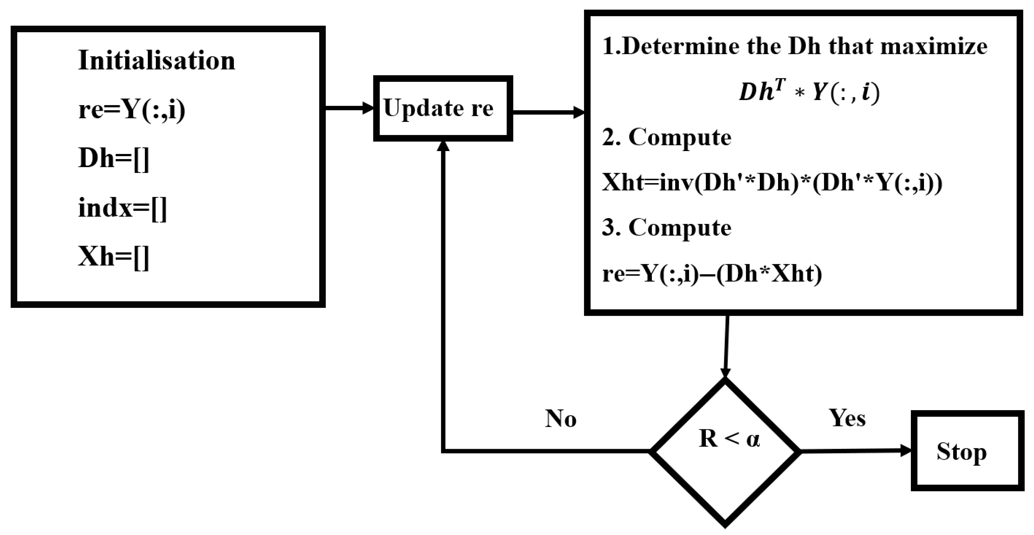
Figure 1 illustrates the algorithm of LS-OMP. The working of the algorithm may be explained as:

• The residue (re) is assigned as the first column of Y; the normalized squared mean (R) is taken and is compared with the product of sparse error constant (S) and a positive constant (eb); this product is represented by α.
• If residue is less than α, then the iteration stops, and the residue is assigned to the next column of Y.
• If the normalized residue (R) is greater than α, then the residue is multiplied with the transposed dictionary and its absolute value is calculated. The dictionary column which will contribute the maximum for the representation of the signal is identified and its column number is added to the index (indx) and the column is added to the temporary dictionary (Dh). The updated dictionary is used to calculate the temporary column of the sparse matrix (Xht). The iterations provide all the non-sparse elements of Xht, which are added to the intermediate sparse matrix (Xh) at appropriate positions.

Figure 1. Flow chart for LS-OMP algorithm.

Figure 1. Flow chart for LS-OMP algorithm.

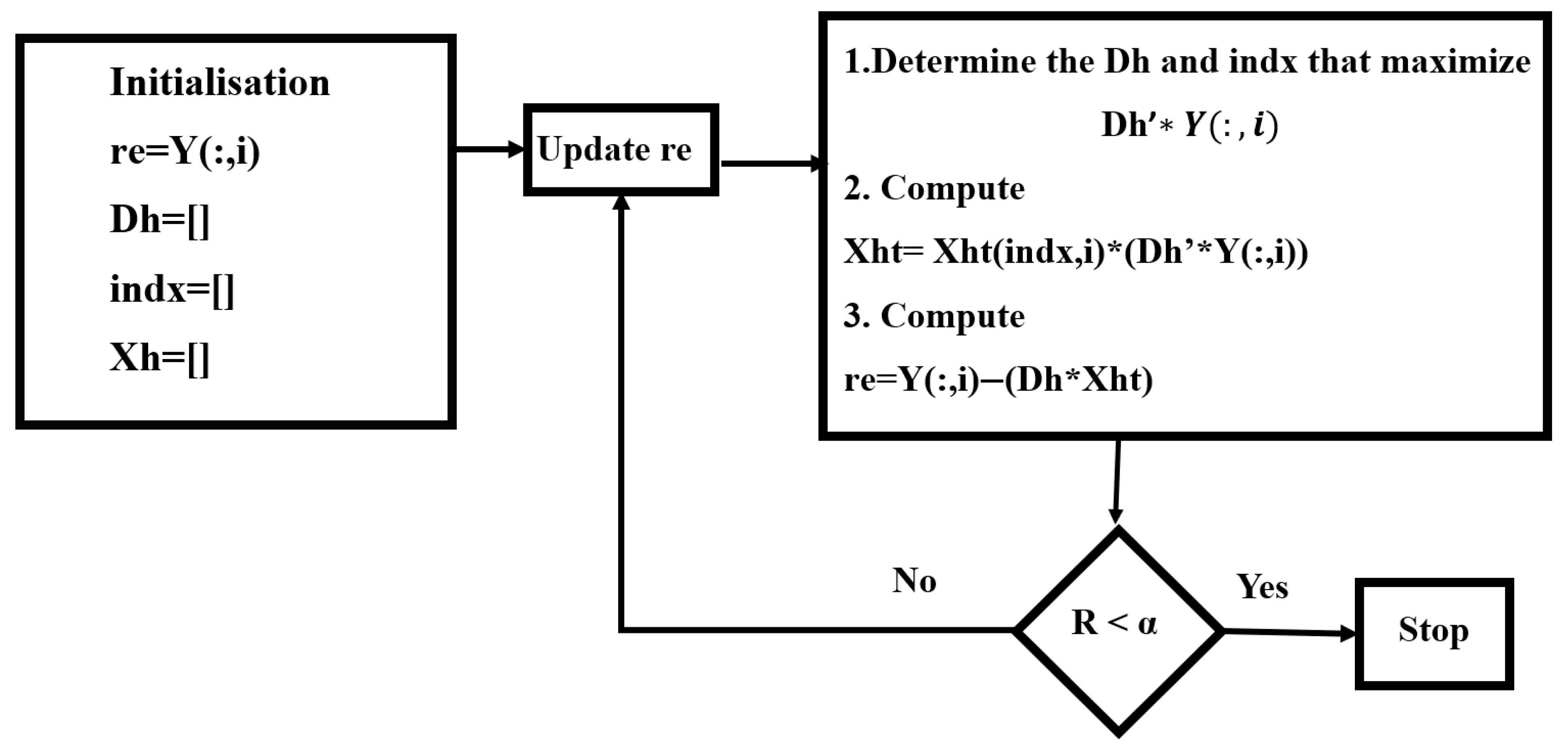
Unlike the OMP algorithm, the residue ‘re’ is used only as a stopping criterion and not for sparse signal generation. Instead, the error between the actual signal and reconstructed signal is calculated at every iteration and is used for sparse signal generation. This makes LS-OMP slower than OMP, but more accurate. In Matching Pursuit (MP), the sparse signal calculation is modified as shown in Figure 2. In this method, the column from the dictionary that contributes the maximum to the representation of the signal is directly chosen for sparse representation. The error is not calculated in each iteration.

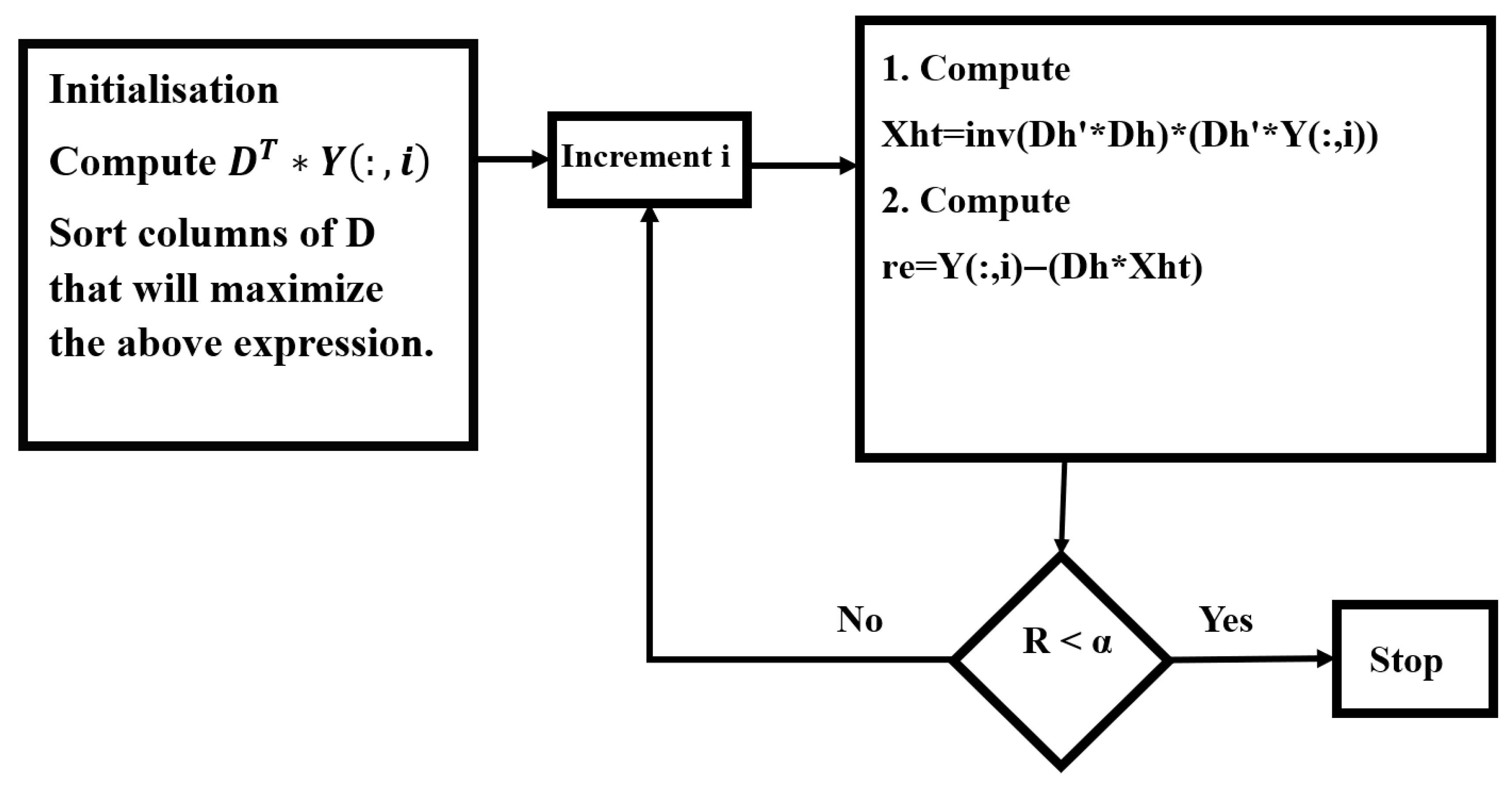
In the Thresholding algorithm as shown in Figure 3, the columns of the dictionary which contributes a maximum for the representation of the actual signal are ordered in descending order. Then, each such column is utilized for the sparse representation in the corresponding step.

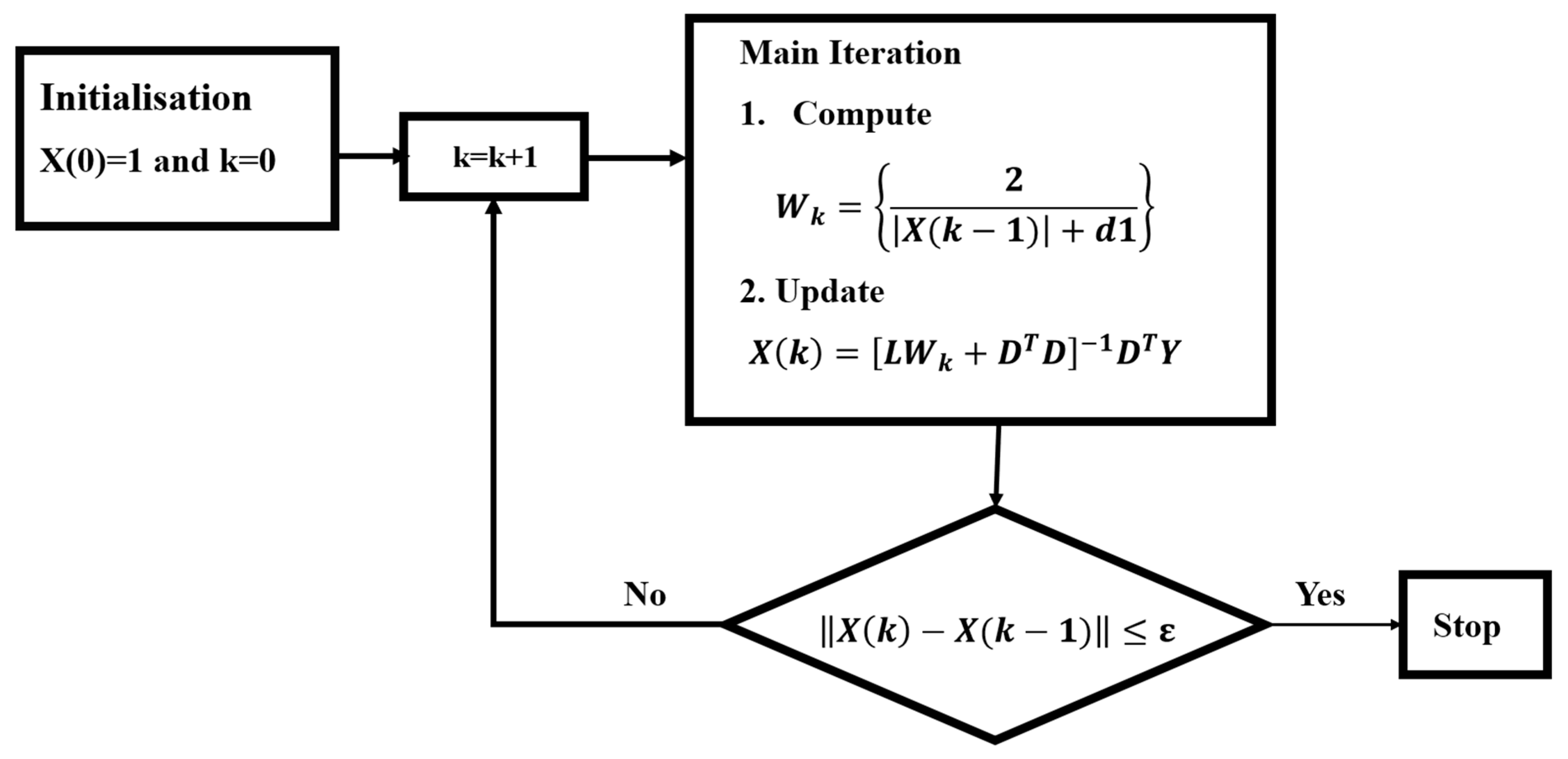
The Basis Pursuit is not based on l₀ norm, it uses l₁ norm for solving Equation (1), i.e., Basis Pursuit minimizes the first norm of the sparse matrix (X), as shown in Equation (4), with the $p_0^{ϵ}$ condition.

$$\widehat{X}=Arg {min}_X{‖X‖}_1 s.t. {‖Y-DX‖}_2\le ϵ$$

(4)

where ${\Vert \Vert }_1$ is the l₁ norm. The problem is to minimize the first norm of X, such that the second norm of Y − DX is less than or equal to a small positive constant ε. The implementation of Basis Pursuit using Iterative Reweighted Least Squares (IRLS) is shown in Figure 4. The diagonal weight matrix W_k is calculated from X as shown in Equation (5):

$$W_k=\left[\begin{array}{c}\begin{array}{ccc}{\displaystyle \frac{2}{\left|X\left(1\right)\right|+d1}}& 0& \dots \\ 0& {\displaystyle \frac{2}{\left|X\left(2\right)\right|+d1}}& \dots \\ 0& 0& {\displaystyle \frac{2}{\left|X\left(3\right)\right|+d1}}\end{array}\begin{array}{cc} 0& 0\\ 0& 0\\ 0& 0\end{array}\\ \begin{array}{ccc}⋮& ⋮& ⋮\\ ⋮& ⋮& ⋮\\ 0& 0& 0\end{array} \begin{array}{cc}\ddots & 0\\ \ddots & 0\\ \dots & {\displaystyle \frac{2}{\left|X\left(m\right)\right|+d1}}\end{array}\end{array}\right]$$

(5)

Here d1 is a small positive constant to avoid division by zero. X will be updated in each step until m steps, where m is the number of columns of Y. L is a small positive constant, which is considered in the constrained least squares problem.

4. Simulation Results

The efficacy of the SSD techniques discussed in the previous sections were evaluated based on accuracy and speed of computation. The techniques with higher accuracy and faster computation speed were considered more suitable for the sparse representation. The stripe representation of the signal was used for computation, as it reduces the dimension of the sparse matrix (X) as compared to treating the signal as a single data set.

In our earlier work [32], a comparative analysis of diverse dictionaries was carried out using OMP as the sole Sparse Signal Decomposition (SSD) technique. The study showed that individual dictionaries, particularly impulse dictionaries, provide better performance than hybrid dictionaries. In addition, an analysis of the sparsity constant—representing the number of columns selected for signal representation—was conducted, and a value of 0.01 was found to yield the best results in terms of accuracy.

Building on these findings, the optimal sparsity constant and individual dictionaries identified in [32] are used for the current analysis. This work focuses on identifying the most effective SSD technique for representing various power quality disturbances with high precision and minimal non-sparse components. The analysis is performed on signals with a fundamental frequency of 50 Hz, with disturbances introduced between 10 s and 50 s.

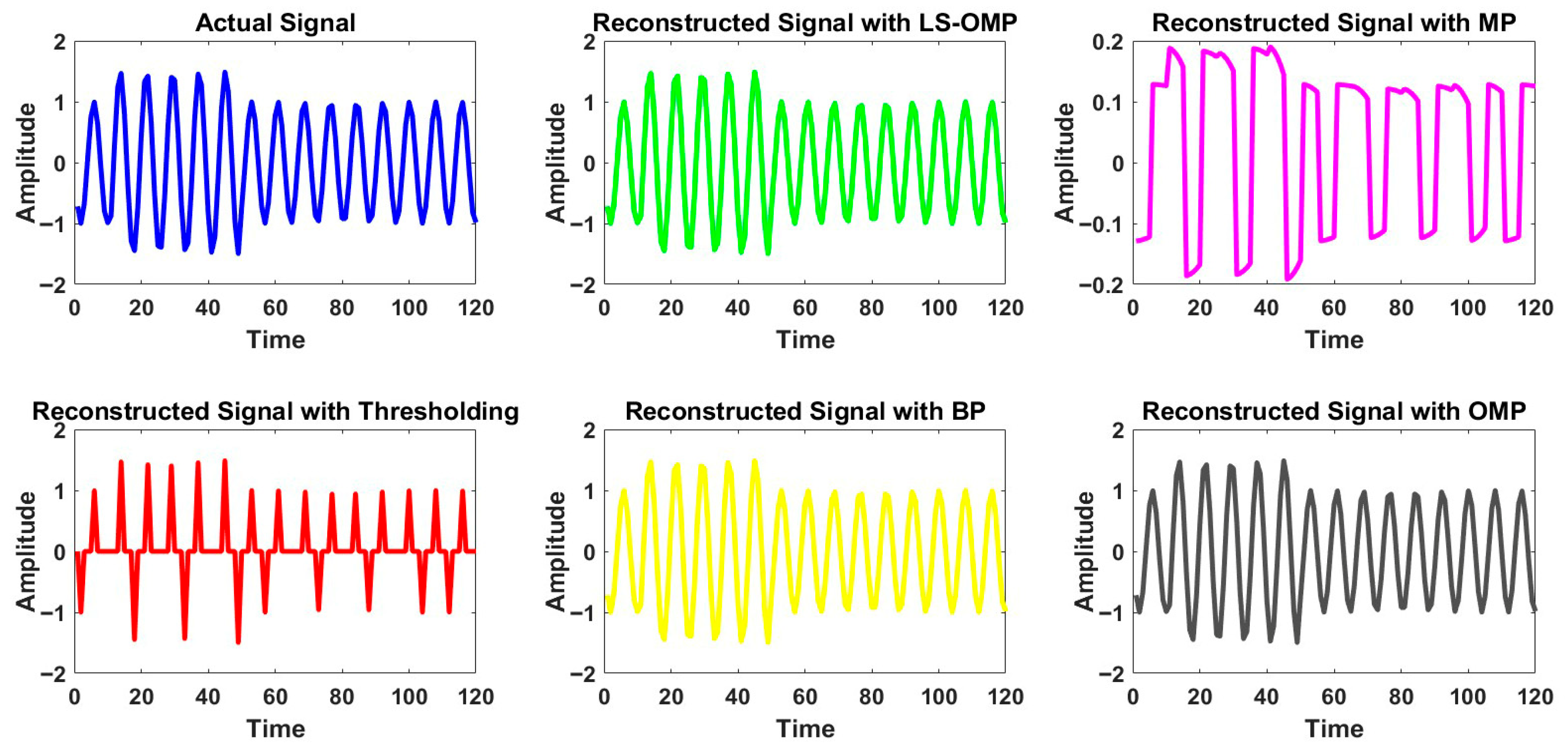
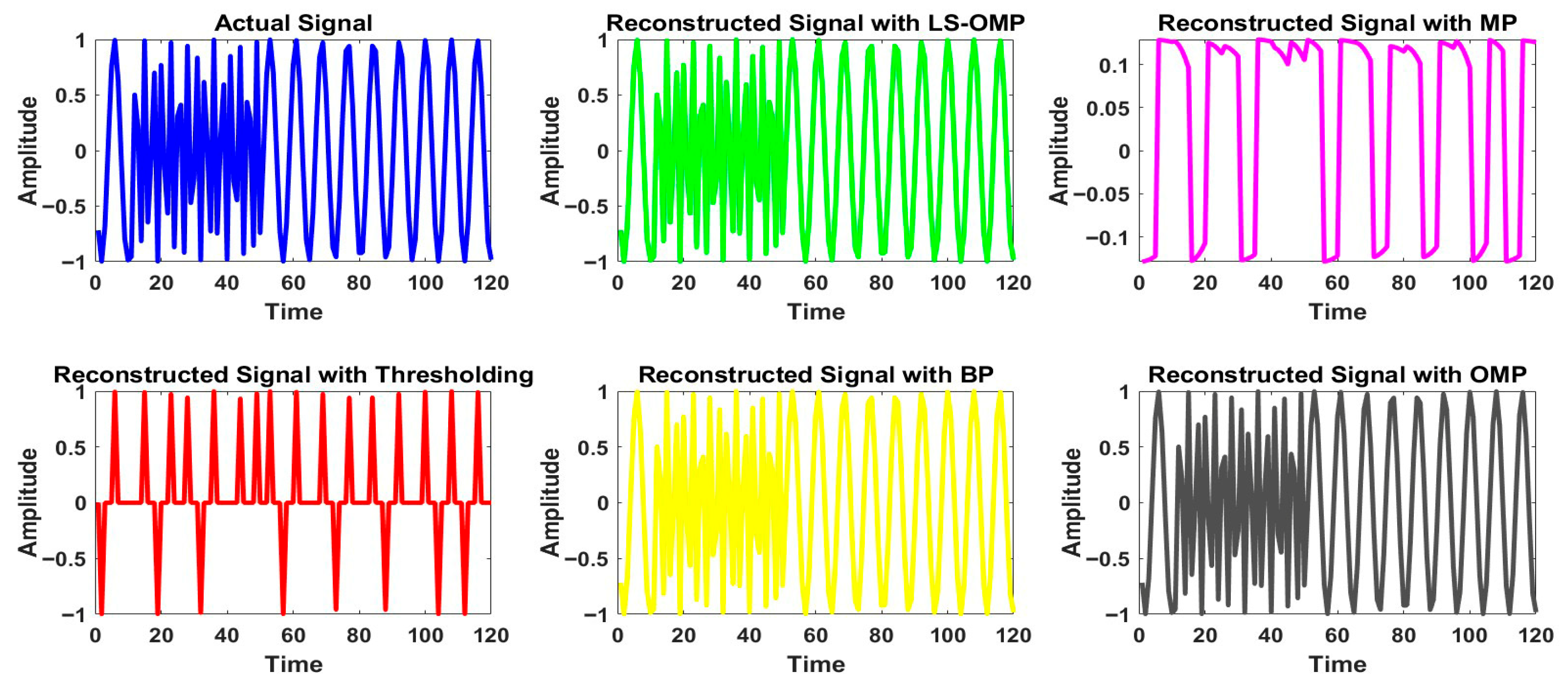
Figure 5 illustrates a power system signal with a swell disturbance (actual signal) along with reconstructed signals obtained using various Sparse Signal Decomposition (SSD) techniques, namely LS-OMP, MP, Thresholding, BP, and OMP with an impulse dictionary. From the figure, it is evident that the reconstructed signals using LS-OMP, BP, and OMP closely match the actual signal, whereas the MP and Thresholding techniques show comparatively poorer reconstruction performance.

Table 1. Performance of SSD techniques for swell disturbance with impulse dictionary.

SSD Technique	Ratio of Actual Signal to Reconstructed Signal (A/R Ratio)	Mean Square Error (MSE)	Percentage Sparsity
MP	3.79	0.3769	87%
Thresholding	1.29	0.1654	86%
Basis Pursuit	1.74 × 10−11	2.58 × 10−24	78%
LS-OMP	0	0	82%
OMP	0	0	82%

presents the reconstruction accuracy and the percentage sparsity of the stored matrix for each method. The results indicate that LS-OMP and OMP achieve perfect reconstruction, with zero A/R ratio and Mean Square Error (MSE) and a reasonably good percentage sparsity of 82%. Although MP attains the highest sparsity of 87%, its A/R ratio and MSE are significantly higher, indicating reduced reconstruction quality.

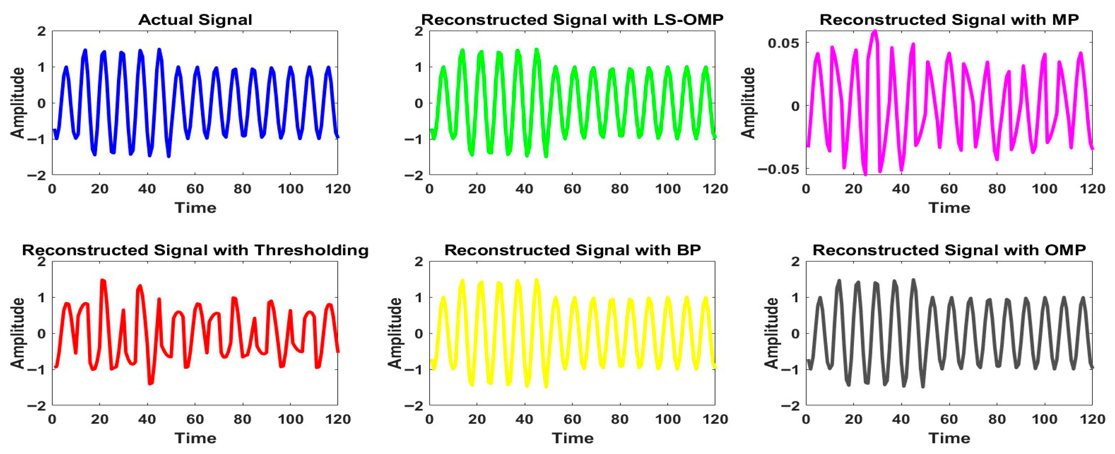
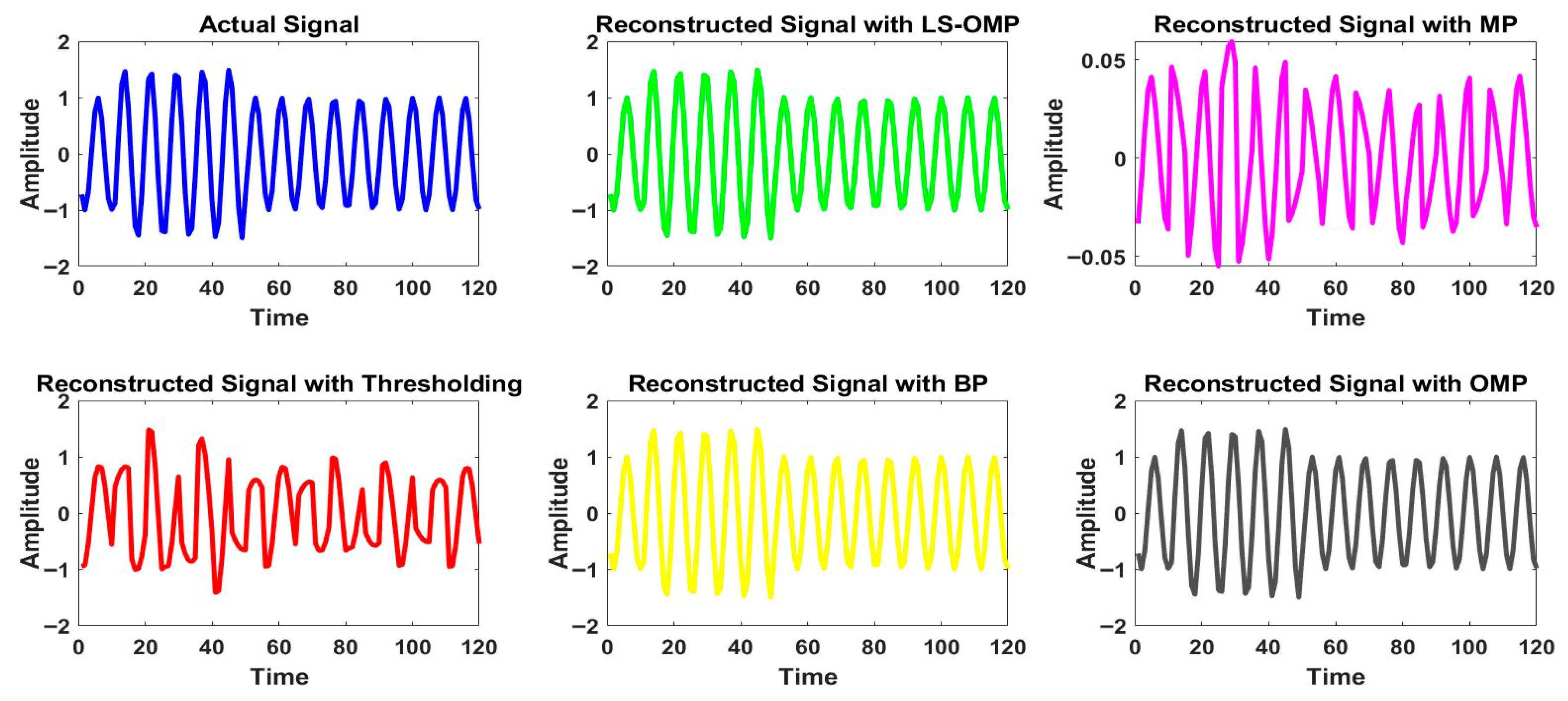
Figure 6 and Figure 7 present the comparison of various SSD techniques for representing swell disturbance using DCT and DST dictionaries, respectively, while

Table 2. Performance of SSD techniques for swell disturbance with DCT dictionary.

SSD Technique	Ratio of Actual Signal to Reconstructed Signal (A/R Ratio)	Mean Square Error (MSE)	Percentage Sparsity
MP	26.32	0.5973	87%
Thresholding	1.30	0.1676	86%
Basis Pursuit	3.21 × 10−4	9.79 × 10−7	78%
LS-OMP	2.68 × 10−7	1.85 × 10−14	82%
OMP	2.67 × 10−7	1.84 × 10−14	82%

and

Table 3. Performance of SSD techniques for swell disturbance with DST dictionary.

SSD Technique	Ratio of Actual Signal to Reconstructed Signal (A/R Ratio)	Mean Square Error (MSE)	Percentage Sparsity
MP	24.90	0.5988	87%
Thresholding	1.36	0.1735	86%
Basis Pursuit	1.6 × 10−3	2.25 × 10−5	78%
LS-OMP	1.04 × 10−6	8.02 × 10−13	82%
OMP	1.02 × 10−6	7.97 × 10−13	82%

summarize the corresponding performance metrics. The observations are consistent with those obtained using the impulse dictionary (Figure 5 and Table 1). In both cases, LS-OMP and OMP yield comparable performance, achieving near-zero A/R ratio and MSE with good sparsity (82%). MP, however, provides the highest sparsity (87%) at the expense of increased reconstruction error.

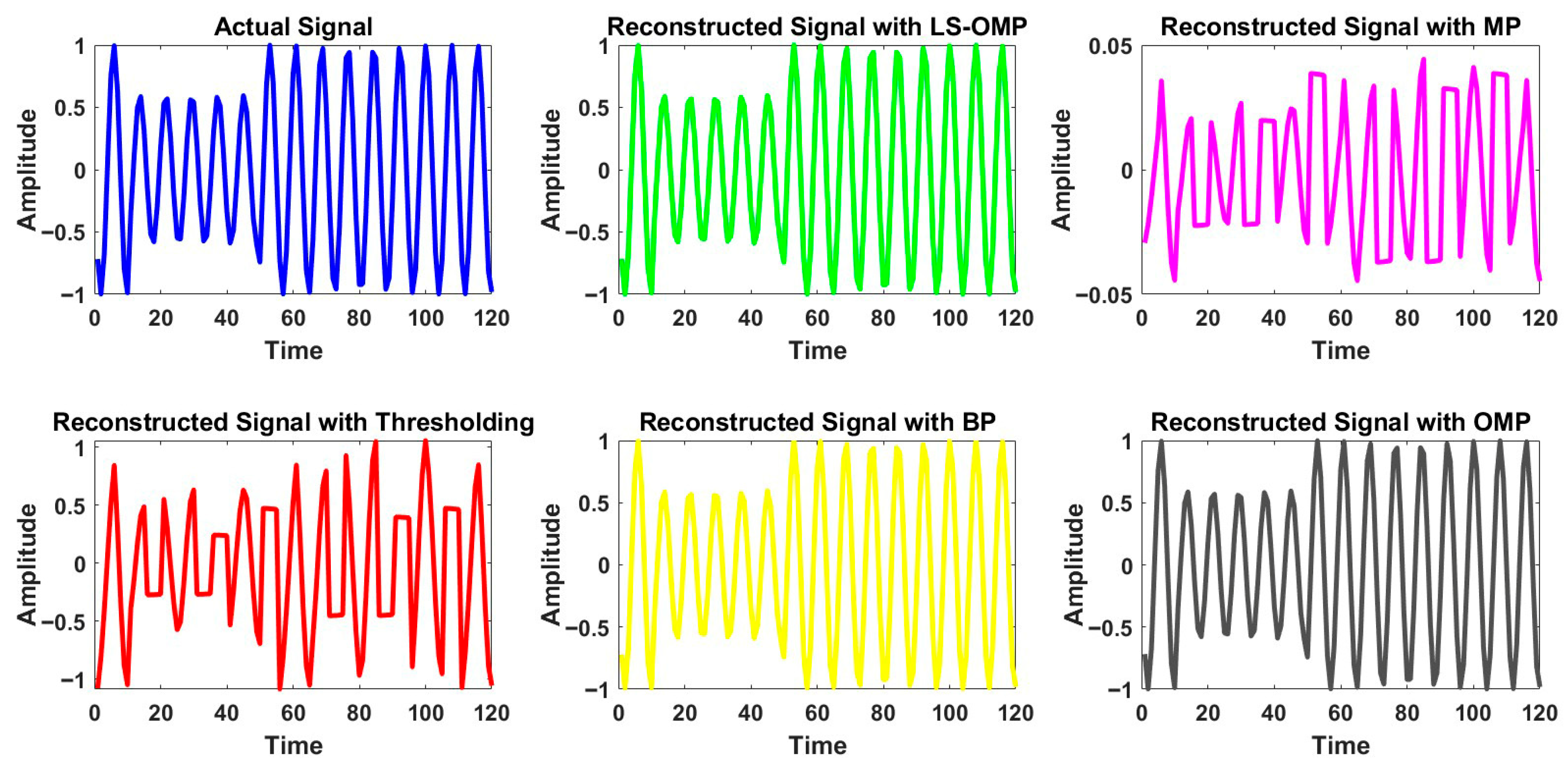
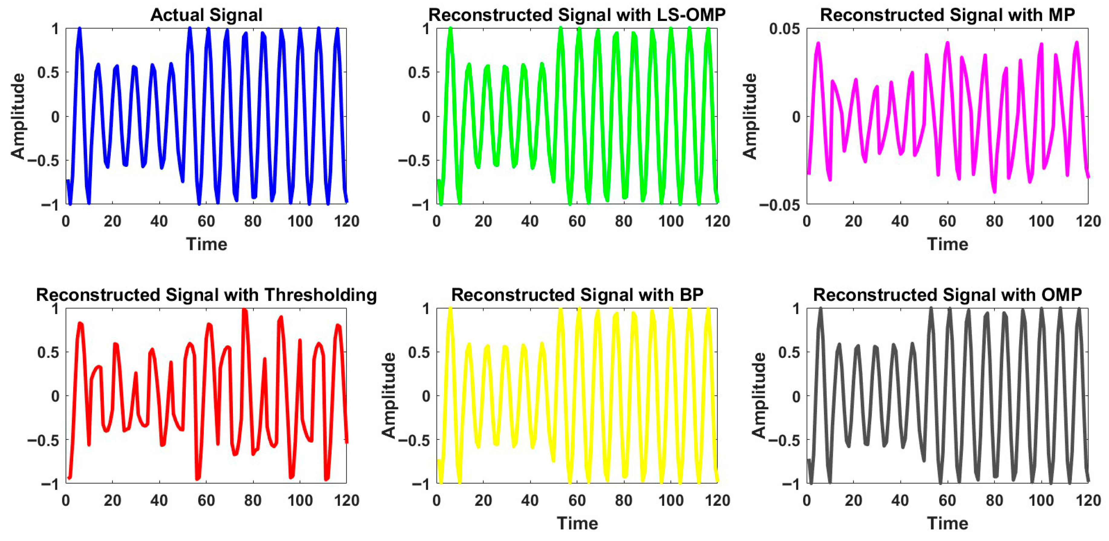
The results presented in Figure 5, Figure 6 and Figure 7 and Table 1, Table 2 and Table 3, indicate that OMP and LS-OMP, with the impulse dictionary, provide the best performance for swell disturbance. A similar comparative study was carried out to reconstruct signals affected by other disturbances such as sag, harmonics, and transients using the same set of algorithms and dictionaries.

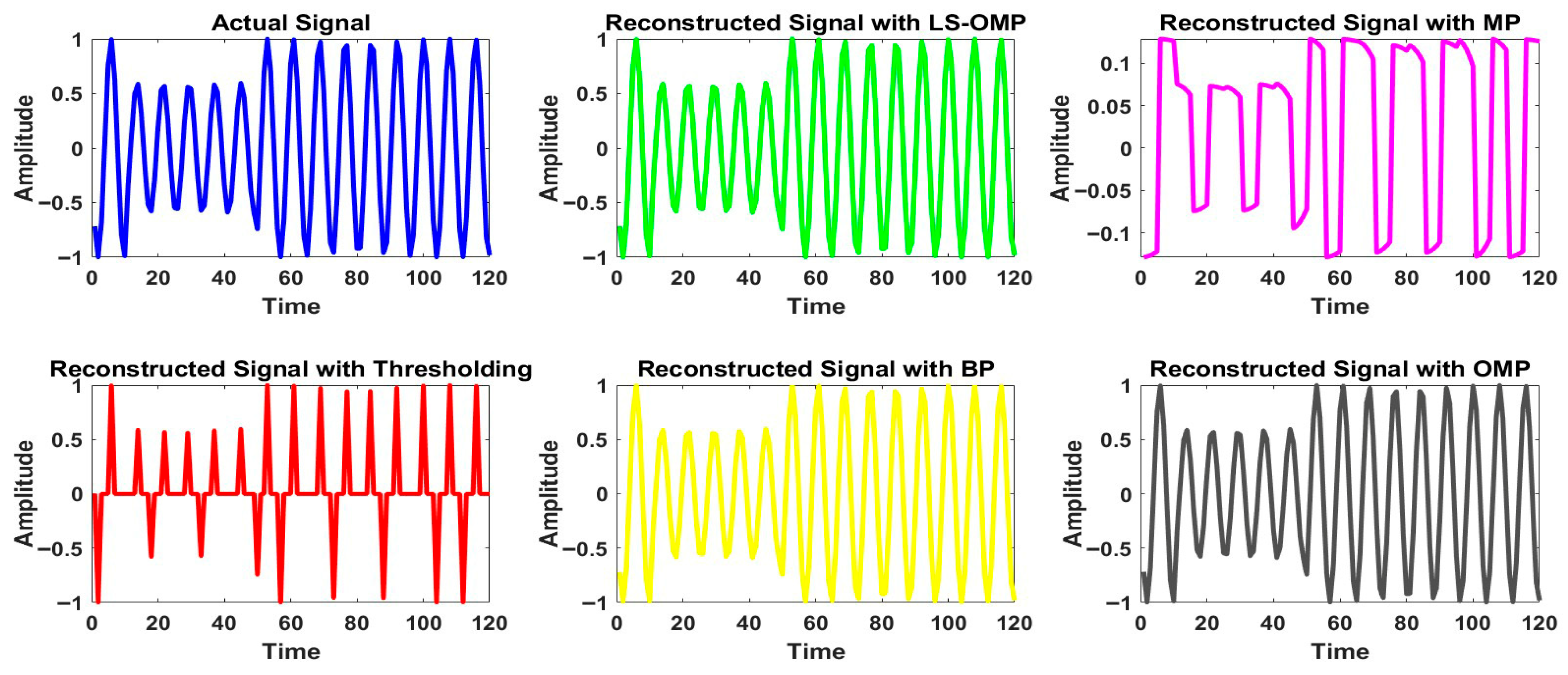
Figure 8, Figure 9 and Figure 10 illustrate the reconstruction results for sag disturbance, while

Table 4. Performance of SSD techniques for sag disturbance with impulse dictionary.

SSD Technique	Ratio of Actual Signal to Reconstructed Signal (A/R Ratio)	Mean Square Error (MSE)	Percentage Sparsity
MP	3.68	0.3755	87%
Thresholding	1.21	0.1454	86%
Basis Pursuit	1.74 × 10−11	2.62 × 10−24	78%
LS-OMP	0	0	82%
OMP	0	0	82%

,

Table 5. Performance of SSD techniques for sag disturbance with DCT dictionary.

SSD Technique	Ratio of Actual Signal to Reconstructed Signal (A/R Ratio)	Mean Square Error (MSE)	Percentage Sparsity
MP	23.94	0.5993	87%
Thresholding	1.41	0.1817	86%
Basis Pursuit	3.57 × 10−4	1.10 × 10−6	78%
LS-OMP	3.43 × 10−7	1.57 × 10−14	82%
OMP	3.24 × 10−7	1.52 × 10−14	82%

and

Table 6. Performance of SSD techniques for sag disturbance with DST dictionary.

SSD Technique	Ratio of Actual Signal to Reconstructed Signal (A/R Ratio)	Mean Square Error (MSE)	Percentage Sparsity
MP	29.30	0.6213	87%
Thresholding	1.24	0.1631	86%
Basis Pursuit	1.7 × 10−3	2.41 × 10−5	78%
LS-OMP	2.38 × 10−7	1.24 × 10−12	82%
OMP	1.78 × 107	1.11 × 10−12	82%

present the corresponding performance metrics in terms of MSE and A/R ratio. As in the case with swell disturbance, the best performance is exhibited by OMP and LS-OMP. The performance of Basis Pursuit, Thresholding and MP is comparatively inferior to LS-OMP and OMP. MP exhibits higher MSE and greater deviation from the actual signal, whereas Thresholding performs better than MP in terms of accuracy but remains less effective than Basis Pursuit and LS-OMP. Basis Pursuit exhibits good accuracy, even though inferior to LS-OMP and OMP, but the main disadvantage is its percentage sparsity. BP has the lowest sparsity (78%) as compared with all the techniques.

Figure 8, Figure 9 and Figure 10 and Table 4, Table 5 and Table 6 further confirm that LS-OMP and OMP, when used with the impulse dictionary, provide the best reconstruction performance for sag disturbance. Basis Pursuit (BP) also yields good results, though with slightly lower accuracy and sparsity compared to LS-OMP and OMP.

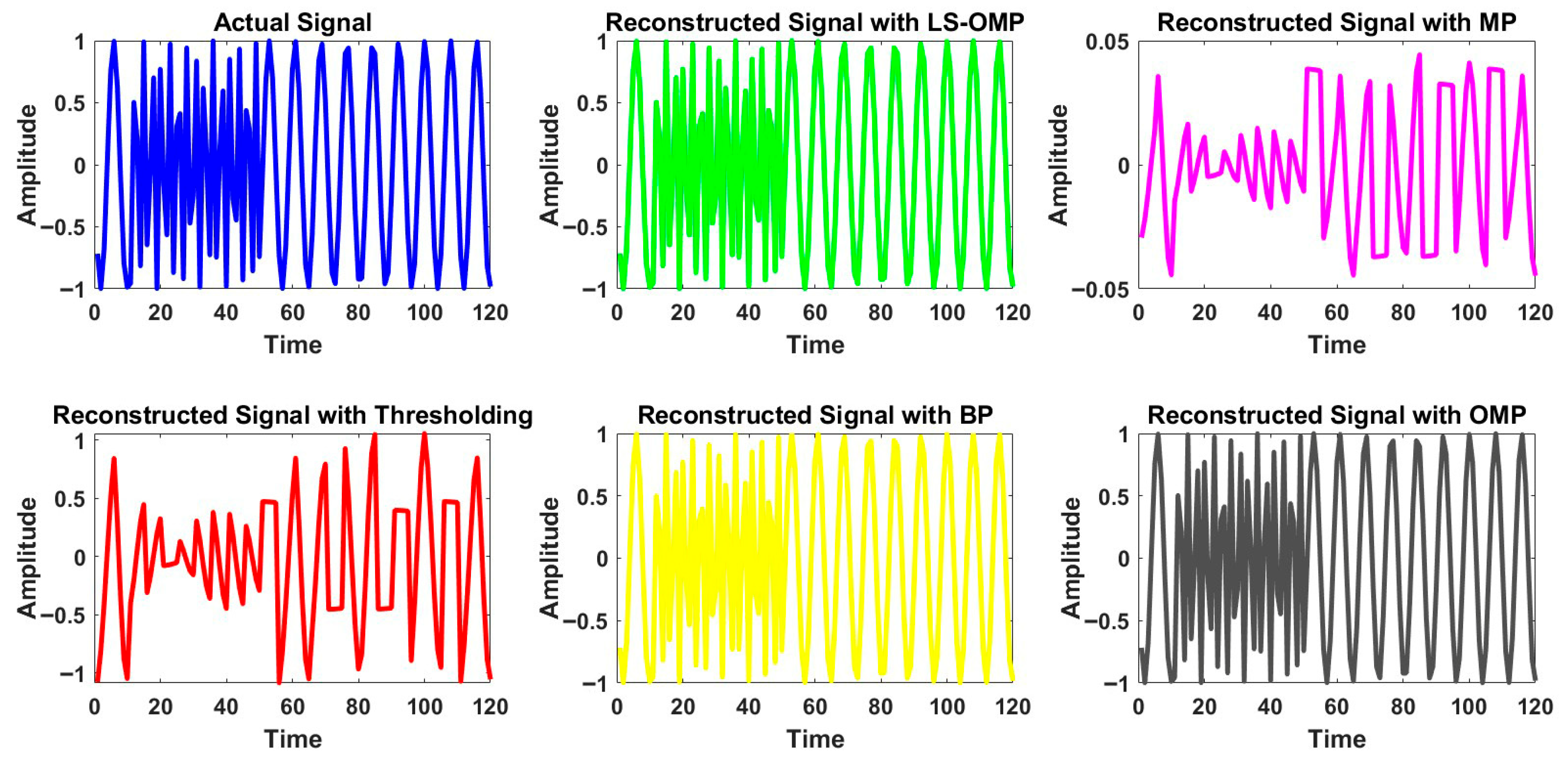
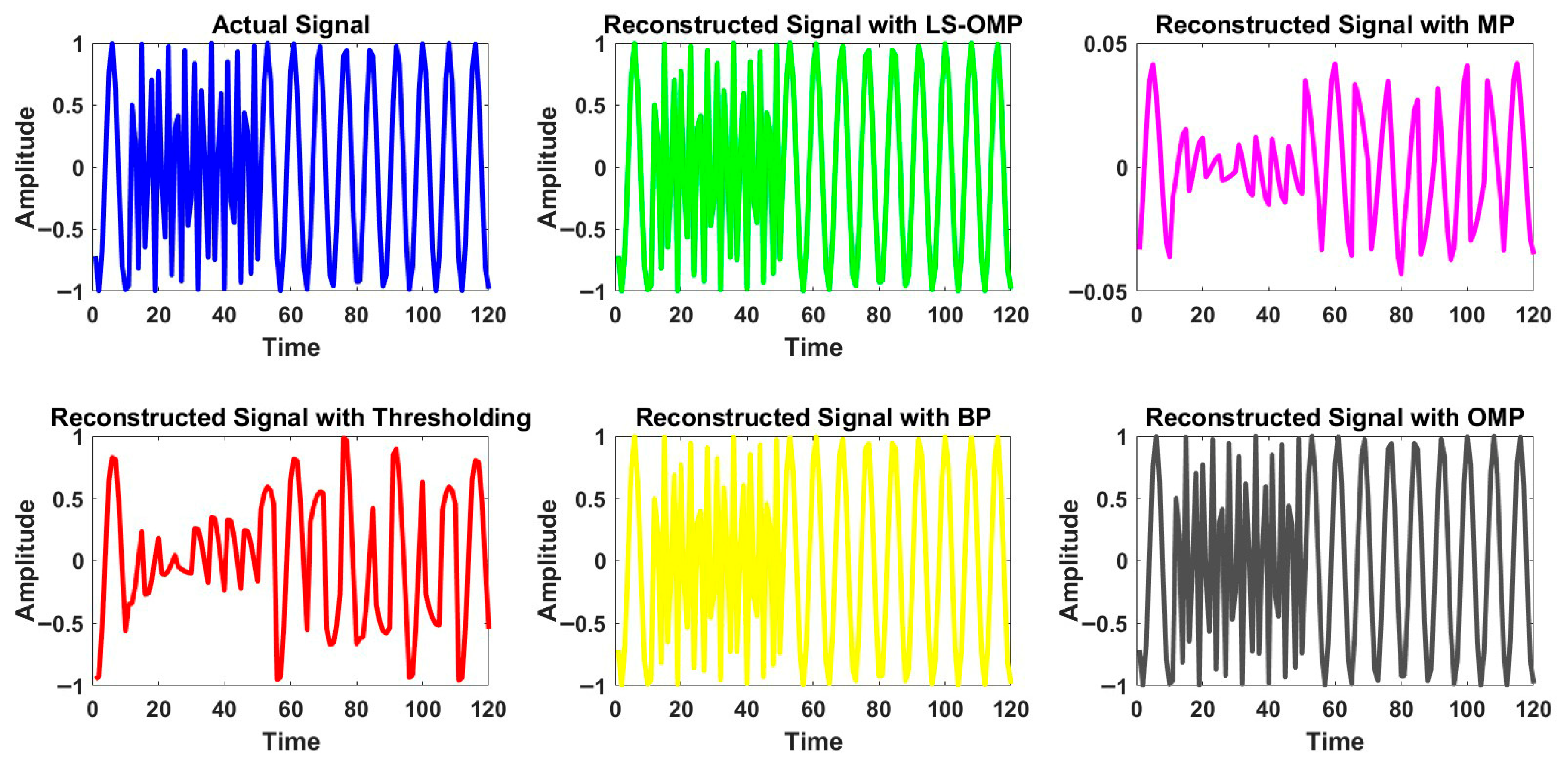
The analysis was then extended to harmonic disturbances, as illustrated in Figure 11, Figure 12 and Figure 13 and

Table 7. Performance of SSD techniques for harmonics disturbance with impulse dictionary.

SSD Technique	Ratio of Actual Signal to Reconstructed Signal (A/R Ratio)	Mean Square Error (MSE)	Percentage Sparsity
MP	15.41	0.4840	87%
Thresholding	4.22	0.3164	86%
Basis Pursuit	1.73 × 10−11	2.03 × 10−24	78%
LS-OMP	5.012 × 10−5	5.88 × 10−6	82%
OMP	4.93 × 10−5	5.56 × 10−6	82%

,

Table 8. Performance of SSD techniques for harmonics disturbance with DCT dictionary.

SSD Technique	Ratio of Actual Signal to Reconstructed Signal (A/R Ratio)	Mean Square Error (MSE)	Percentage Sparsity
MP	29.05	0.4842	87%
Thresholding	2.49	0.2221	86%
Basis Pursuit	3.7 × 10−2	8.74 × 10−5	78%
LS-OMP	3.50 × 10−7	2.25 × 10−14	82%
OMP	3.45 × 10−7	2.14 × 10−14	82%

and

Table 9. Performance of SSD techniques for harmonics disturbance with DST dictionary.

SSD Technique	Ratio of Actual Signal to Reconstructed Signal (A/R Ratio)	Mean Square Error (MSE)	Percentage Sparsity
MP	30.48	0.4924	87%
Thresholding	3.04	0.2561	86%
Basis Pursuit	0.1462	0.0015	78%
LS-OMP	8.12 × 10−7	6.76 × 10−13	82%
OMP	7.67 × 10−7	6.24 × 10−13	82%

. For harmonics, although LS-OMP and OMP remain the most effective SSD techniques, their combination with the DCT dictionary produces better results compared to the impulse dictionary.

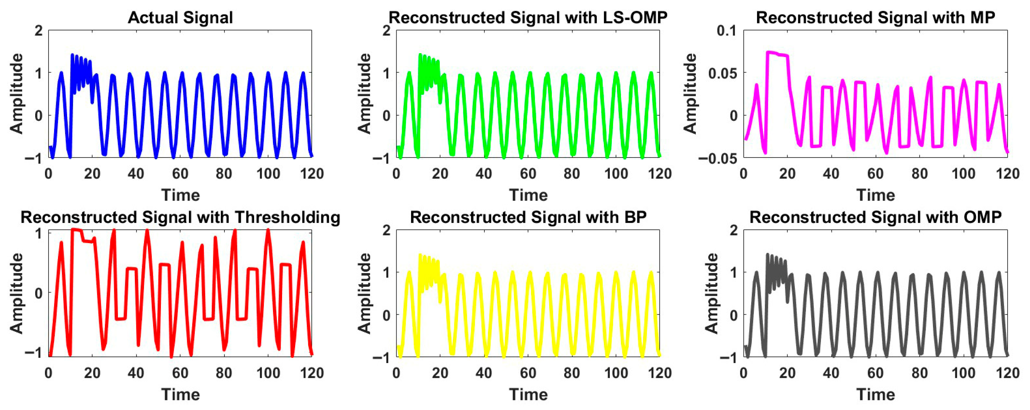
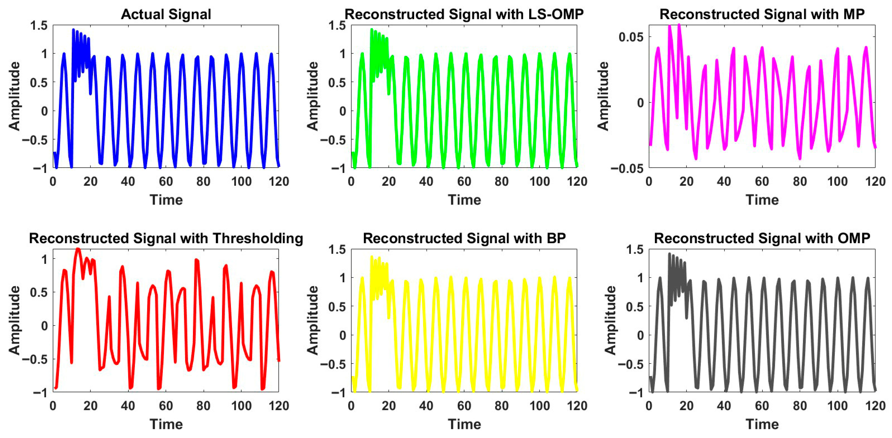
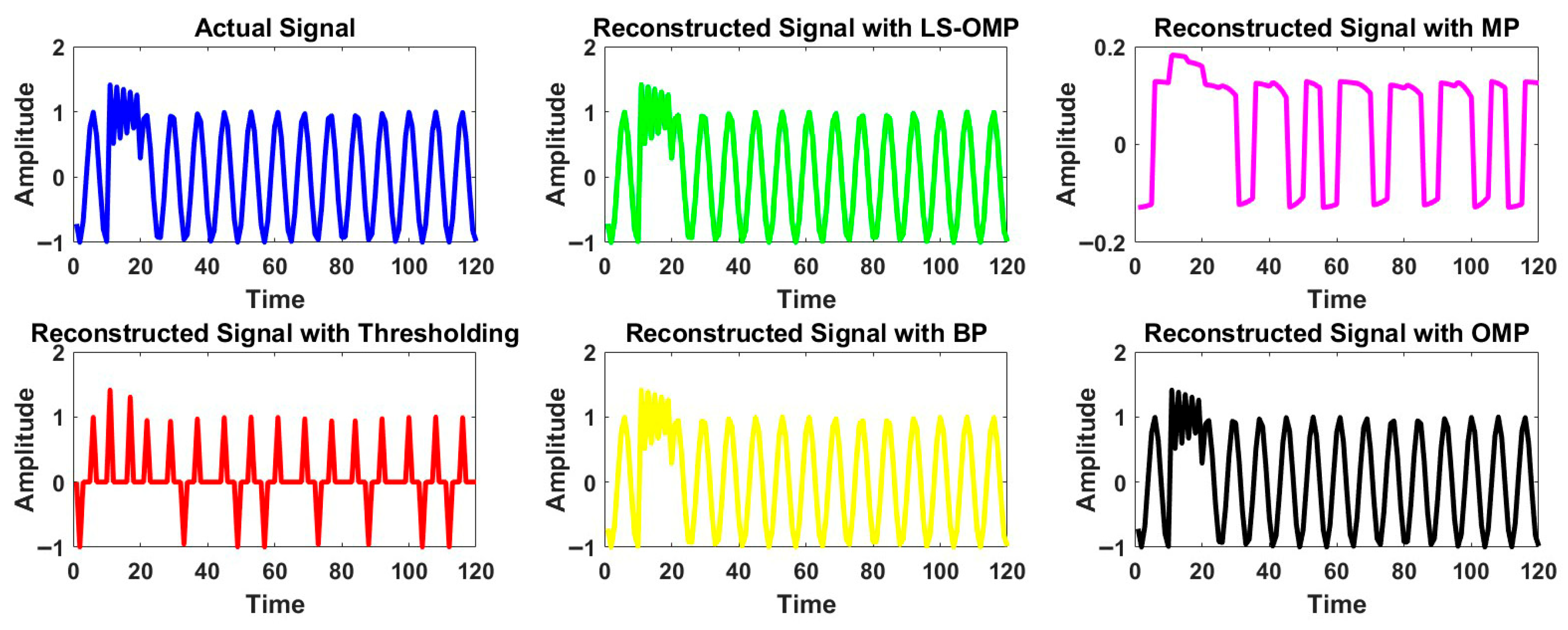
An analysis of the signal with transient disturbance was also conducted, as shown in Figure 14, Figure 15 and Figure 16 and

Table 10. Performance of SSD techniques for transient disturbance with impulse dictionary.

SSD Technique	Ratio of Actual Signal to Reconstructed Signal (A/R Ratio)	Mean Square Error (MSE)	Percentage Sparsity
MP	30.68	0.8755	87%
Thresholding	4.08	1.02	86%
Basis Pursuit	1.73 × 10−11	6.72 × 10−24	78%
LS-OMP	0	0	82%
OMP	0	0	82%

,

Table 11. Performance of SSD techniques for transient disturbance with DCT dictionary.

SSD Technique	Ratio of Actual Signal to Reconstructed Signal (A/R Ratio)	Mean Square Error (MSE)	Percentage Sparsity
MP	32.94	0.8993	87%
Thresholding	1.37	0.4565	86%
Basis Pursuit	5.01 × 10−4	3.87 × 10−6	78%
LS-OMP	8.03 × 10−7	9.63 × 10−14	82%
OMP	7.88 × 10−7	9.31 × 10−14	82%

and

Table 12. Performance of SSD techniques for transient disturbance with DST dictionary.

SSD Technique	Ratio of Actual Signal to Reconstructed Signal (A/R Ratio)	Mean Square Error (MSE)	Percentage Sparsity
MP	29.30	0.8213	87%
Thresholding	1.85	0.5852	86%
Basis Pursuit	0.0036	1.30 × 10−4	78%
LS-OMP	8.40 × 10−6	1.27 × 10−11	82%
OMP	8.23 × 10−6	1.18 × 10−11	82%

. The results are consistent with those observed for sag and swell disturbances, where LS-OMP and OMP, along with the impulse dictionary, provide the best accuracy with reasonably good sparsity.

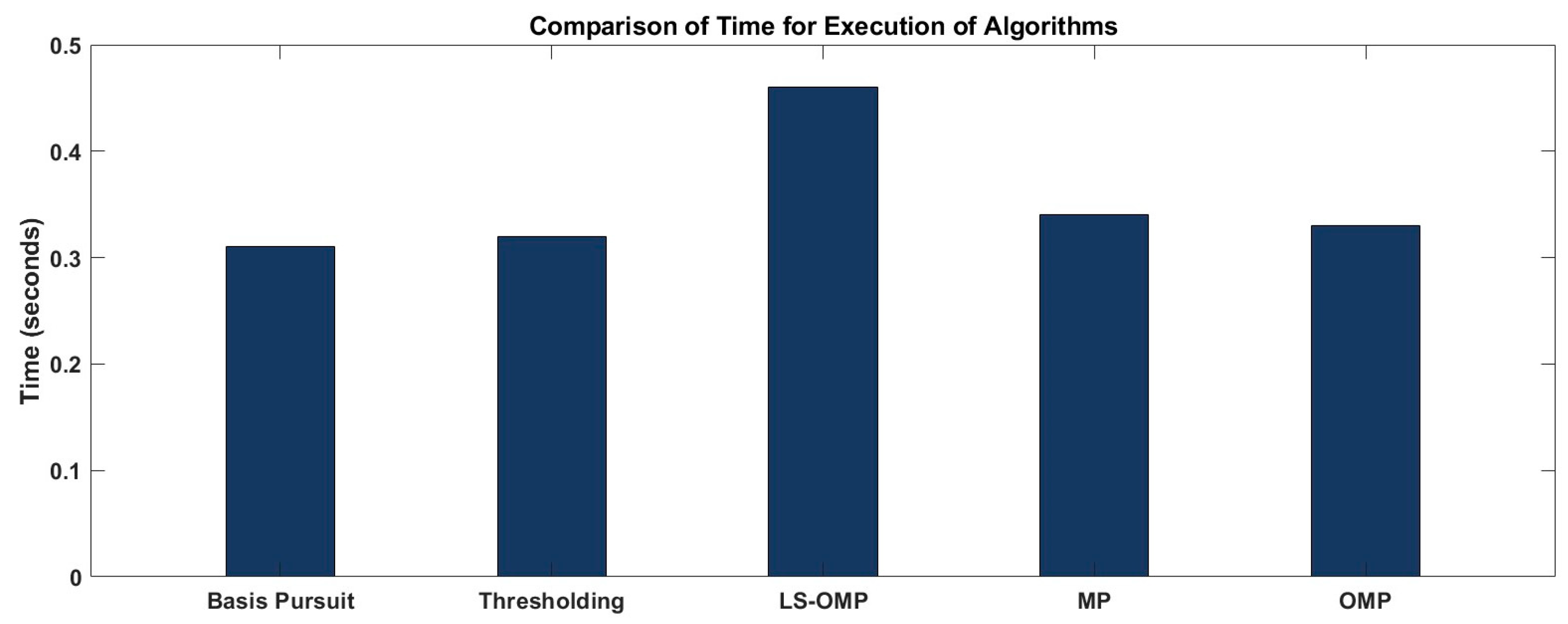
From the analysis, it is found that the choice of dictionary has a significant role on the accuracy of sparse representation. The LS-OMP and OMP with impulse dictionary is found to be the best option for representing all disturbance signals except harmonics. DCT dictionary provided better accuracy for signals with harmonics. An analysis on time of computation of techniques were also done as shown in Figure 17. All the techniques had similar time of computation, which was around 0.3 s, with LS-OMP having a slightly higher computation time.

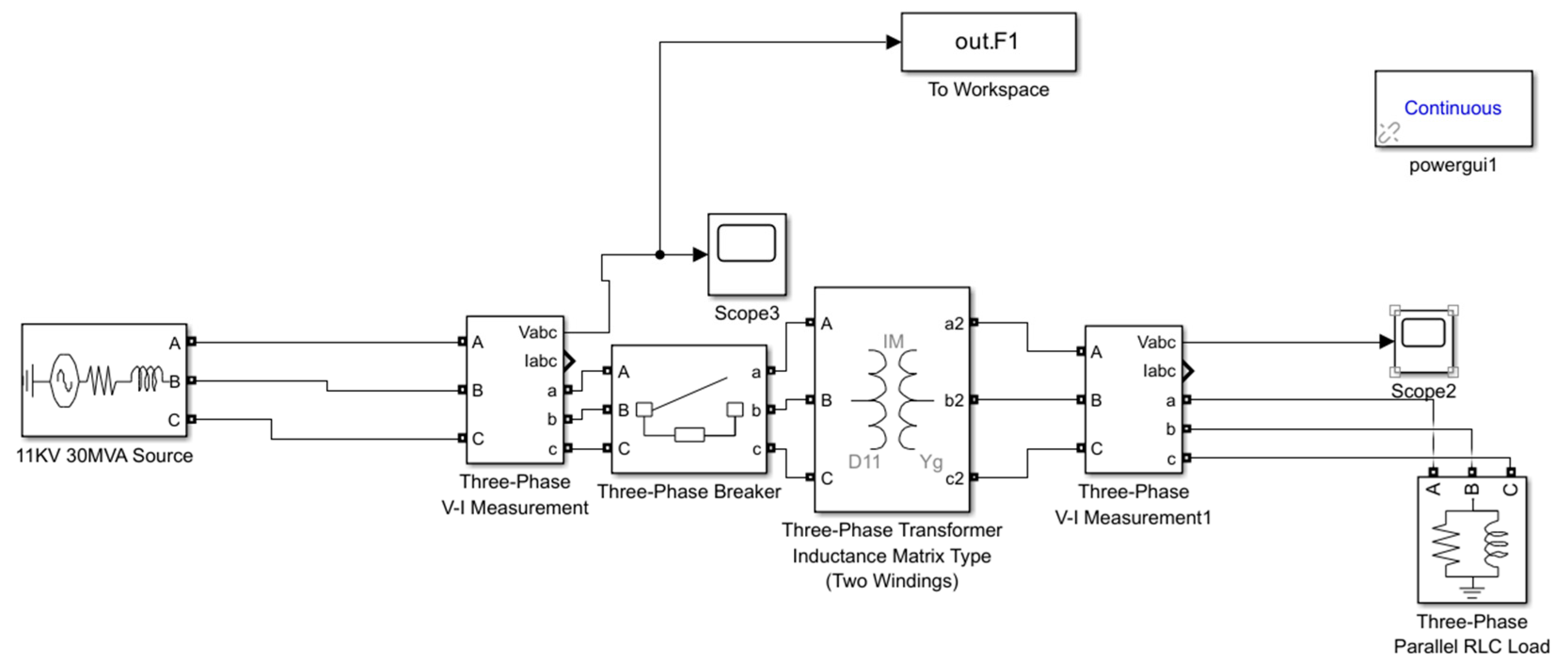
The analysis presented in the previous section was carried out using synthetic data generated from mathematical models of power quality disturbances. To validate these results, power quality disturbance signals were also generated using a MATLAB/Simulink (R2023b) model, as shown in Figure 18. The model, adopted from [37], represents a standard power system configuration that produces a voltage sag disturbance when the transformer is switched on. The resulting voltage signal was exported and analyzed using different SSD techniques.

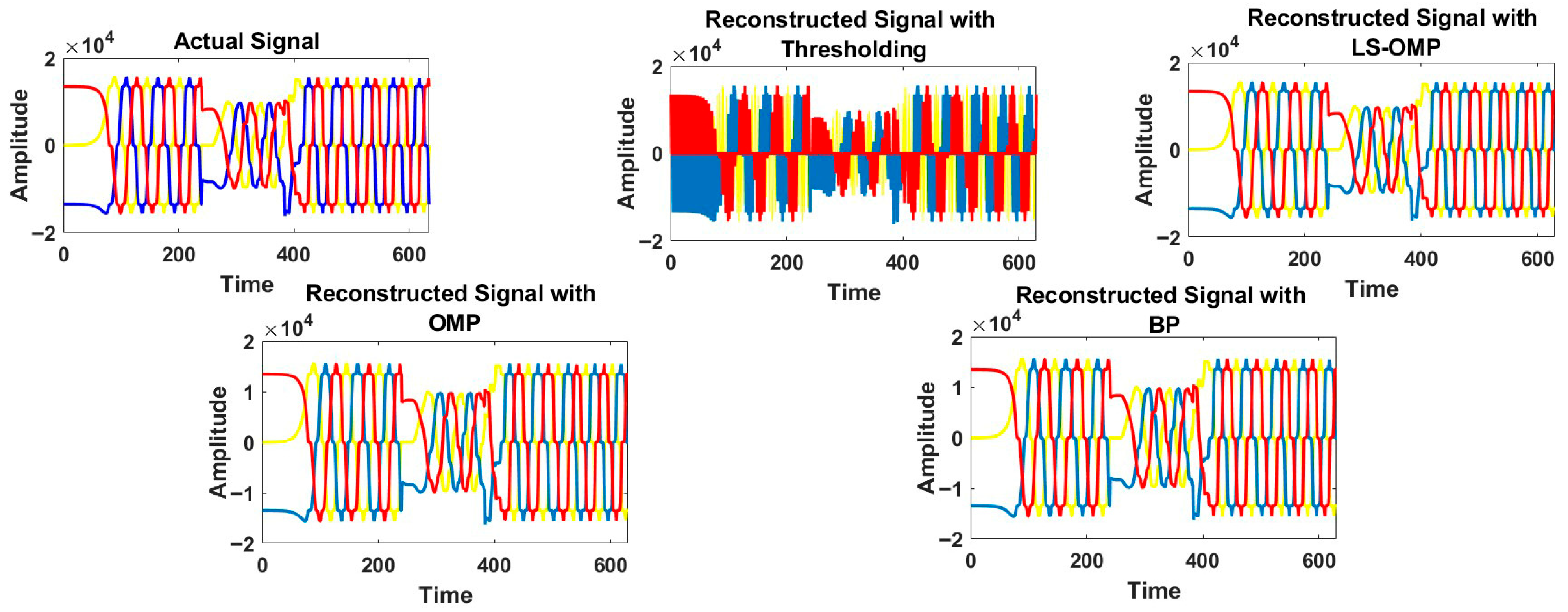
The results represented in Figure 19 indicate that LS-OMP and OMP provide accurate reconstruction of the signal, with near-zero MSE and A/R ratio. The corresponding performance metrics are presented in

Table 13. Performance of SSD techniques for signal obtained from Simulink model.

SSD Technique	Ratio of Actual Signal to Reconstructed Signal (A/R Ratio)	Mean Square Error (MSE)	Percentage Sparsity
Thresholding	5.9943	7.74	86%
Basis Pursuit	1.73 × 10−11	4.13 × 10−16	78%
LS-OMP	0	0	82%
OMP	0	0	82%

. Since the Simulink-generated signals exhibit accuracy and memory requirements comparable to those obtained with synthetic data, these results serve as a validation of the findings of this study.

The performance of sparse decomposition techniques in the analysis proved that all the power signals, even with disturbances, can be represented in sparse form with precision by suitably choosing the sparse decomposition technique, with the appropriate dictionary. This could contribute to developing a framework that will store signal data in the most precise and efficient way.

5. Conclusions

This paper examined different Sparse Signal Decomposition techniques to identify the most suitable method for representing power quality disturbance signals with high accuracy and reduced data size. The results show that for disturbances such as sag, swell, and transients, both OMP and LS-OMP perform well when used with an impulse dictionary. These combinations provide high reconstruction accuracy along with lower memory requirements due to better sparsity.

When computation time is also considered, OMP has a clear advantage over LS-OMP, making it the more efficient choice overall. Therefore, for achieving a good balance of accuracy, sparsity, and computation speed, OMP with an impulse dictionary is found to be the most effective approach for most disturbance types.

However, for harmonic signals, the results indicate that the DCT dictionary performs better than the impulse dictionary for greedy algorithms. The relaxation algorithm (Basis Pursuit) along with impulse dictionary provided better accuracy for representing signals with harmonics. This signifies the requirement for choosing the apt technique for representing the signal, depending on the type of disturbances.

The study highlights that both the choice of sparse recovery technique and the selection of dictionary is important for the optimized representation of the power quality disturbance signal. Choosing the right combination based on the type of disturbance can lead to efficient and accurate signal representation. This could aid in developing a framework that can store power signal data with maximum precision and minimum memory requirements. These data can then be sent to monitoring centres, so that they can take appropriate action effectively and easily, as the data they have to process will be less.

References

1. Manikandan, M.S.; Samantaray, S.R.; Kamwa, I. Detection and Classification of Power Quality Disturbances Using Sparse Signal Decomposition on Hybrid Dictionaries. IEEE Trans. Instrum. Meas. 2015, 64, 27–38. [Google Scholar] [CrossRef]
2. Karimi-Ghartemani, M.; Bakshai, A.; Eren, S. New generation of signal processing techniques for power system applications. In Proceedings of the 2007 IEEE Canada Electrical Power Conference, EPC 2007, Montreal, QC, Canada, 25–26 October 2007; IEEE: Piscataway, NJ, USA, 2017; pp. 256–260. [Google Scholar]
3. Wang, J.; Kwon, S.; Li, P.; Shim, B. Recovery of sparse signals via generalized orthogonal matching pursuit: A new analysis. IEEE Trans. Signal Process. 2016, 64, 1076–1089. [Google Scholar] [CrossRef]
4. Elad, M. Sparse and Redundant Representations: From Theory to Application in Signal and Image Processing; Springer: New York, NY, USA, 2010; pp. 1–376. [Google Scholar]
5. Aharon, M.; Elad, M.; Bruckstein, A. K-SVD: An Algorithm for Designing Overcomplete Dictionaries for Sparse Representation. IEEE Trans. Signal Process. 2006, 54, 4311–4322. [Google Scholar] [CrossRef]
6. Rubinstein, R.; Bruckstein, A.M.; Elad, M. Dictionaries for Sparse Representation Modeling. Proc. IEEE 2010, 98, 1045–1057. [Google Scholar] [CrossRef]
7. Qayyum, A.; Malik, A.S.; Naufal, M.; Saad, M.; Mazher, M.; Abdullah, F.; Abdullah, T.A.R.B.T. Designing of overcomplete dictionaries based on DCT and DWT. In Proceedings of the 2015 IEEE Student Symposium in Biomedical Engineering & Sciences (ISSBES), Shah Alam, Malaysia, 4 November 2015. [Google Scholar]
8. Bruckstein, A.M.; Donoho, D.L.; Elad, M. From sparse solutions of systems of equations to sparse modeling of signals and images. SIAM Rev. 2009, 51, 34–81. [Google Scholar] [CrossRef]
9. Liu, X.; Xia, S.; Fu, F. Reconstruction Guarantee Analysis of Basis Pursuit for Binary Measurement Matrices in Compressed Sensing. IEEE Trans. Inf. Theory 2017, 63, 2922–2932. [Google Scholar] [CrossRef]
10. Li, H.; Liu, G. Perturbation Analysis of Signal Space Fast Iterative Hard Thresholding with Redundant Dictionaries. IET Signal Process. 2017, 11, 462–468. [Google Scholar] [CrossRef]
11. Stanković, L.; Sejdić, E.; Stanković, S.; Daković, M.; Orović, I. A Tutorial on Sparse Signal Reconstruction and Its Applications in Signal Processing. Circuits Syst. Signal Process. 2019, 38, 1206–1263. [Google Scholar] [CrossRef]
12. Liu, X.; Liu, B.; Xu, D. Recognition and classification of power quality disturbances on the basis of pattern linguistic values. J. Electr. Eng. Technol. 2016, 11, 309–319. [Google Scholar] [CrossRef][Green Version]
13. Ray, P.; Budumuru, G.K.; Mohanty, B.K. A comprehensive review on soft computing and signal processing techniques in feature extraction and classification of power quality problems. J. Renew. Sustain. Energy 2018, 10, 025102. [Google Scholar] [CrossRef]
14. Wang, Q.; Pang, C.; Qian, C. Sparse Dictionary Learning for Transient Stability Assessment. Front. Energy Res. 2022, 10, 932770. [Google Scholar] [CrossRef]
15. Kathirvel, P.; Manikandan, M.S.; Maya, P.; Soman, K.P. Detection of power quality disturbances with overcomplete dictionary matrix and ℓ1-norm minimization. In Proceedings of the International Conference on Power and Energy Systems, Chennai, India, 22–24 December 2011; IEEE: Piscataway, NJ, USA, 2011; pp. 1–6. [Google Scholar]
16. Chawda, G.S.; Shaik, A.G.; Shaik, M.; Padmanaban, S.; Holm-Nielsen, J.B.; Mahela, O.P.; Kaliannan, P. Comprehensive Review on Detection and Classification of Power Quality Disturbances in Utility Grid with Renewable Energy Penetration. IEEE Access 2020, 8, 146807–146830. [Google Scholar] [CrossRef]
17. Ruiz, M.; Montalvo, I. Electrical Faults Signals Restoring Based on Compressed Sensing Techniques. Energies 2020, 13, 2121. [Google Scholar] [CrossRef]
18. Chandran, L.R.; Karuppasamy, I.; Nair, M.G.; Sun, H.; Krishnakumari, P.K. Compressive Sensing in Power Engineering: A Comprehensive Survey of Theory and Applications, and a Case Study. J. Sens. Actuator Netw. 2025, 14, 28. [Google Scholar] [CrossRef]
19. Oubrahim, Z.; Amirat, Y.; Benbouzid, M.; Ouassaid, M. Power Quality Disturbances Characterization Using Signal Processing and Pattern Recognition Techniques: A Comprehensive Review. Energies 2023, 16, 2685. [Google Scholar] [CrossRef]
20. Khetarpal, P.; Tripathi, M.M. A critical and comprehensive review on power quality disturbance detection and classification. Sustain. Comput. Inform. Syst. 2020, 28, 100417. [Google Scholar] [CrossRef]
21. Papyan, V.; Sulam, J.; Elad, M. Working Locally Thinking Globally: Theoretical Guarantees for Convolutional Sparse Coding. IEEE Trans. Signal Process. 2017, 65, 5687–5701. [Google Scholar] [CrossRef]
22. Ge, S.-C.; Zhou, S. Nonstationary signal extraction based on BatOMP sparse decomposition technique. Sci. Rep. 2021, 11, 17869. [Google Scholar] [CrossRef]
23. Ge, S.; Gao, Z.; Li, J.; Zhang, X.; Huang, W.; Feng, K.; Zhang, C.; Sun, J. Novel sparse decomposition with adaptive evolutionary atoms for nonstationary signal extraction. Sci. Rep. 2025, 15, 39744. [Google Scholar] [CrossRef]
24. Huang, B.; Song, K.; Jiang, S.; Zhao, Z.; Zhang, Z.; Li, C.; Sun, J. A Robust Salp Swarm Algorithm for Photovoltaic Maximum Power Point Tracking Under Partial Shading Conditions. Mathematics 2024, 12, 3971. [Google Scholar] [CrossRef]
25. Battula, V.V.R.; Padmavathi, K.; Sravanthi, K. Comparison of advanced signal decomposition techniques for the classification of PQDs by machine learning algorithms. Sci. Rep. 2025, 15, 38164. [Google Scholar] [CrossRef]
26. Zaman, W.; Siddique, M.F.; Khan, S.U.; Kim, J.-M. A new dual-input CNN for multimodal fault classification using acoustic emission and vibration signals. Eng. Fail. Anal. 2025, 221, 110216. [Google Scholar] [CrossRef]
27. Sun, S.; Wang, Q.; Yan, H.; Lin, X.; Du, T. Application of EEMD in power harmonic detection. Proc. CSU-EPSA 2024, 28, 25–31. [Google Scholar]
28. Gong, Z.; Zou, Y.; Jin, T.; Liu, Y.; Lan, M.; Liu, Z. Power Quality Disturbance Classification Method Based on Feature Fusion Parallel Optimization Model. Proc. CSEE 2023, 43, 1017–1027. [Google Scholar]
29. Xiao, D.; Liu, J.; Liu, H.; Zhao, Y. A Lightweight Method for Power Quality Disturbance Recognition Based on Optimized VMD and CNN–Transformer. Electronics 2026, 15, 1832. [Google Scholar] [CrossRef]
30. Zhang, J.; Yang, S.; Yang, Y.; Yuan, Y.; Wang, X. A Hybrid Forecasting Framework with Adaptive Parameter Optimization and Multi-Scale Feature Fusion for Non-Stationary Power Grid CPS Time Series. J. Electr. Eng. Technol. 2026, 21, 1–22. [Google Scholar] [CrossRef]
31. Liu, K.; Han, J.; Chen, S.; Ruan, L.; Liu, Y.; Wang, Y. Power quality disturbance identification method based on improved CEEMDAN-HT-ELM model. Processes 2025, 13, 137. [Google Scholar] [CrossRef]
32. Anjali, V.; Panikker, P.P.K. Investigation of the Effect of Diverse Dictionaries and Sparse Decomposition Techniques for Power Quality Disturbances. Energies 2024, 17, 6152. [Google Scholar] [CrossRef]
33. Fu, Y.; Zhu, T.; Xiang, Y.; Chen, Z.; Cai, L. Stability Analysis of ℓ0,∞-Norm Based Convolutional Sparse Coding Using Stripe Coherence. IEEE Trans. Signal Process. 2020, 68, 5810–5823. [Google Scholar] [CrossRef]
34. Ahmed, I.; Khalil, A.; Ahmed, I.; Frnda, J. Sparse Signal Representation, Sampling, and Recovery in Compressive Sensing Frameworks. IEEE Access 2022, 10, 85002–85018. [Google Scholar] [CrossRef]
35. Chakraborty, S.; Chatterjee, A.; Goswami, S.K. A sparse representation-based approach for recognition of power system transients. Eng. Appl. Artif. Intell. 2014, 30, 137–144. [Google Scholar] [CrossRef]
36. Dabou, R.T.; Kamwa, I.; Tagoudjeu, J.; Mugombozi, F.C. Sparse Signal Reconstruction on Fixed and Adaptive Supervised Dictionary Learning for Transient Stability Assessment. Energies 2021, 14, 7995. [Google Scholar] [CrossRef]
37. Tan, R.H.G.; Ramachandaramurthy, V.K. A Comprehensive Modeling and Simulation of Power Quality Disturbances Using MATLAB/SIMULINK. In Power Quality Issues in Distributed Generation; InTech: London, UK, 2015. [Google Scholar] [CrossRef]
Figure 2. Flow chart for MP algorithm.
Energies 19 02399 g002
Figure 3. Flow chart for Thresholding algorithm.
Energies 19 02399 g003
Figure 4. Flow chart for Basis Pursuit algorithm.
Energies 19 02399 g004
Figure 5. Comparison of diverse SSD techniques for representing swell disturbance using impulse dictionary.
Energies 19 02399 g005
Figure 6. Comparison of diverse SSD techniques for representing swell disturbance using DCT dictionary.
Energies 19 02399 g006
Figure 7. Comparison of diverse SSD techniques for representing swell disturbance using DST dictionary.
Energies 19 02399 g007
Figure 8. Comparison of diverse SSD techniques for representing sag disturbance using impulse dictionary.
Energies 19 02399 g008
Figure 9. Comparison of diverse SSD techniques for representing sag disturbance using DCT dictionary.
Energies 19 02399 g009
Figure 10. Comparison of diverse SSD techniques for representing sag disturbance using DST dictionary.
Energies 19 02399 g010
Figure 11. Comparison of diverse SSD techniques for representing harmonics disturbance using impulse dictionary.
Energies 19 02399 g011
Figure 12. Comparison of diverse SSD techniques for representing harmonics disturbance using DCT dictionary.
Energies 19 02399 g012
Figure 13. Comparison of diverse SSD techniques for representing harmonics disturbance using DST dictionary.
Energies 19 02399 g013
Figure 14. Comparison of diverse SSD techniques for representing transient disturbance using impulse dictionary.
Energies 19 02399 g014
Figure 15. Comparison of diverse SSD techniques for representing transient disturbance using DCT dictionary.
Energies 19 02399 g015
Figure 16. Comparison of diverse SSD techniques for representing transient disturbance using DST dictionary.
Energies 19 02399 g016
Figure 17. Comparison of execution time of SSD algorithms.
Energies 19 02399 g017
Figure 18. Simulink model for sag disturbance.
Energies 19 02399 g018
Figure 19. Comparison of diverse SSD techniques for representing signal obtained from the Simulink model.
Energies 19 02399 g019