A Guideline for Developing Time Series Forecasting Models to Predict Industrial Energy Demands

Abstract

Forecasting energy demand is crucial in industry to increase energy use efficiency and reduce greenhouse gas emissions. Although extensive research has been conducted in this field, it is still challenging for industrial companies to identify suitable methods for forecasting energy demand. Therefore, a new categorisation of energy forecasting models is developed in this paper. This categorisation is based on the available data and not on the methodology, as is usually the case. Thus, the intention is to make it easier to create a forecasting model and to identify the appropriate methodology. It also indicates what is needed to improve the forecast. The focus of this paper is on forecasting energy demand in industrial companies. To facilitate application, a guideline is established. The guideline describes which methodologies can be used based on the available data. The development of the guideline is based on various research projects for which forecasting models are created. The guideline starts with simple forecasting methods and gradually increases in complexity, including examples for each forecasting method. In addition, the methods available for each forecasting category are specified, and references are made to the relevant literature. After the description of the guideline, further explanation is provided on how the created forecasting model can be checked and integrated into a continuous improvement process.

1. Introduction

The need to achieve European climate targets, the geopolitical situation and changes in the energy supply due to the reinforced integration of renewables are increasing energy prices in Europe and increasing price variability. Therefore, it is essential for European industries to utilise the available energy efficiently. Various technologies and optimisation processes are needed to reduce industrial energy requirements. The foundation for this is understanding industrial processes and how they can be optimised to reduce the energy demand and/or shift the demand to times when energy prices are favourable. For this, it is essential to forecast the future energy demand to carry out accurate planning. This paper focuses on forecasting the future energy demand of industrial companies.

Forecasts can be used for different applications; thus, there are various forecasting methods and categorisations. The areas of application for forecasting are, according to Islam et al. [1], the following:

• Optimum supply schedule: The forecast of the future energy demand allows power producers to dispatch power optimally, reducing risks of additional costs of under- or oversupply.
• Fuel mix selection: The forecast of the future energy demand facilitates the planning of fuel supplies and the selection of fuel mix for power plants.
• Power plant and network planning: Energy demand forecasting is essential for deciding on the size, location, route, and types of future power plants as well as power transmission and distribution networks.
• Demand-side management: Energy demand forecasting allows utilities or policymakers to structure plans for managing demand through incentives, penalties, and other demand management measures.
• Renewable planning: Energy demand forecasting facilitates decisions on the location and size of renewable energy generation plants.

Time series forecasting is commonly used to forecast energy demand. In time series forecasting, an entire time series is forecast, not only a single time step [2]. The number of time steps to be forecast depends on the forecasting horizon and the resolution of the time series. The forecasting horizon and the resolution of the time series differ according to the application. The forecasting horizon can range from a few minutes to days, weeks, months or years. Similarly, the resolution of the time series can range from seconds or minutes to hours and days. Higher resolutions of the time series are rather unusual in the energy sector.

Furthermore, the availability of data is decisive in selecting appropriate forecasting methods. There are three different possibilities for data availability:

• Only energy demand data from the past are available (historical energy demand).
• Additional data are available for the past and the future time horizon (historical energy demand + historical and future additional data).
• The additional data are only available for the past and not for the future time horizon to be forecast (historical energy demand + historical additional data).

These additional data consist of various parameters that influence the energy demand, such as the ambient temperature, production plan, shift plan, maintenance schedule etc. The additional data can differ for every industrial use case. Parameters having an influence in a steel company can be irrelevant for an automobile plant. Furthermore, it is also crucial whether the additional data can be measured and predicted. In industry, it frequently occurs that during the development of energy forecasts, parameters with a high influence on the energy demand are identified, but there are no recorded data. It is even more difficult to have a reliable prediction of the additional data. It then remains questionable whether a prediction of the additional data is possible or cost-effective. Often, these predictions are too expensive for industry and other methods must be used. Which method fits best and when is explained in Section 4.4. For example, Zawodnik et al. [3] identified that the scrap quality has a significant influence on the energy demand of an electric arc furnace, but there is no prediction of the scrap quality available, so a combined forecasting approach (see Section 4.5.2) is used. For the prediction of the additional data, it must be considered that the predicted additional data can change or deviate from the prediction. Hence, the accuracy of the energy demand forecast model depends on the reliability of the prediction of the additional data. The prediction of the additional data is assumed to be deterministic. In this work, only deterministic forecasts are considered. As data availability in European industry is currently limited, stochastic approaches are hardly feasible. This work focuses on practical solutions in industry. Further research is needed into how stochastic approaches can be implemented in industry and under which conditions they are beneficial.

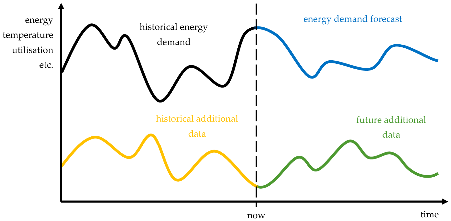
Figure 1 illustrates the three different possibilities for data availability. The difference between a forecast based solely on historical energy demand data and a forecast with additional data is also called a univariate or multivariate forecast [4]. The multivariate forecast describes forecasting methods in which additional data are considered. However, multivariate forecasts do not differ between historical additional and future additional data. Nevertheless, it is essential to distinguish between these two cases for the guideline established in Section 4. Therefore, the subdivision, as shown in Figure 1, is used. The blue curve represents the energy demand, which needs to be forecast. The black one is the corresponding energy demand from the past. These data are at least necessary to predict the future energy demand. The additional data (input parameters) are represented in yellow and green. The yellow curve is the available additional data in the past, and the green curve is the available additional data from the future. In Figure 1, only one input parameter for the additional data is represented. For the forecast, more than one input parameter can be used.

Industrial companies need to determine which methods are best suited to forecasting their energy demand while considering their specific process characteristics. For this purpose, this paper develops a guideline that describes which methods are best suited for creating a forecasting model based on the available data. The guideline focuses on time series forecasting of industrial energy demand. An additional limitation is that the guideline is designed for a forecasting horizon of between a few minutes and a week, with time resolutions of one minute to one hour. Whether the guideline can be used beyond these restrictions remains to be investigated.

2. State of Research

Forecasts play an essential role in energy system engineering. They often form the basis for various optimisation procedures and system analyses (e.g., demand-side management, operational optimisation, control systems, validation of different scenarios, building air conditioning and other energy loads, etc.). This is why an increasing amount of research is being carried out on energy demand forecasting. Technologies such as artificial intelligence and enhanced hardware capabilities also offer new forecasting possibilities that require investigation. This leads to an increased need for research in this area. 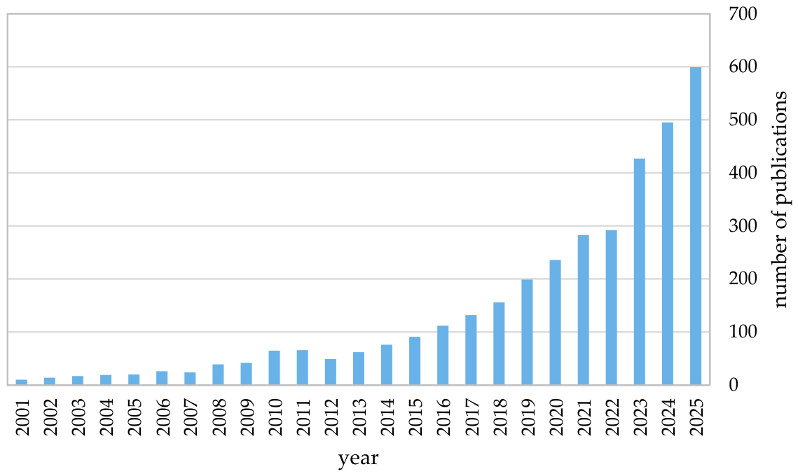Figure 2 shows the increasing interest in forecasting methods in energy research. Figure 2 illustrates the number of published articles on energy demand forecasting. This steady increase in publications emphasises the necessity for research into energy demand forecasting.

Current research focuses on applying new technologies to various problems, defining their advantages and disadvantages, and comparing them with existing forecasting methods. In addition, the forecasting methods are analysed based on their methods and assigned to the respective categories. The review papers by Deb et al. [5], Klyuev et al. [6] and Makridakis et al. [7] present investigations of different forecasting methods. It is noted that current scientific research focuses on the design of methods and their improvement and refinement. For example, Li et al. [8] and Zawodnik et al. [3] investigated which methods are best to improve the forecast or to find the best operation strategy in an energy system. This research is important, and further research is needed in this area, but it is criticised that a uniform terminology is not available. A holistic classification of the various methods is lacking. However, forecasting methods are mainly categorised according to the type of method, prediction horizon and time resolution. Classifications according to the area of application (buildings, industry, energy sector, transport, etc.), the basis of the data availability (which data are available for the forecast), industry sectors or other categorisation criteria are rarely considered.

Deb et al. [5] show how much research has already been carried out in the building sector and the corresponding methods used. In comparison, not as much research has been performed in the industrial sector. Klyuev et al. [6] mention the lack of research to determine which forecasting method suits the industry sector. The methods are always used individually and adapted to the specific problems. According to Klyuev et al. [6], a general analysis of the forecasting methods for usage in industry is still lacking. Furthermore, the quality and applicability of a forecast model is still strongly dependent on the knowledge of the person who builds the model [9].

This work is intended to contribute to a holistic categorisation of energy demand forecasting methods that are especially suitable for industrial processes. In contrast to previous works, the categorisation of forecasting methods is not based on the type of forecast but on the available data. Data availability has a more decisive influence on the forecasting method compared to, for example, the industry sector. A guideline was developed to make the industry’s application as easy as possible.

The central research question in this paper is as follows: “Can a guideline be developed that, based on data availability, indicates which method is most suitable for forecasting industrial energy demand?” The following restrictions apply to the guideline:

• Only methods for time series forecasting are considered. Several time steps are required for the further use of the forecast.
• The forecasting horizon ranges from minutes over several hours and days to a maximum of one week. Forecasts outside this range are not analysed in this paper.
• The resolution of the time steps is between one minute and one hour. Lower or higher resolutions are not investigated.
• The guideline refers to industrial companies that want to forecast the energy demand of their production processes.

Unlike previous research, this study introduces a new classification dimension. The focus is on the data available. Depending on the data available, different methods must be used, which are assigned to the relevant categories. The guideline is based on these findings and is designed to help industrial companies identify the appropriate method for forecasting energy demand based on data availability.

3. Methodology

The guideline originates from six projects carried out in collaboration with industry partners. During the implementation of these projects, it became apparent that the data available to the industry partners varied considerably. Consequently, the methods used to forecast energy demand had to be adapted to the specific circumstances of each individual project. To better select the appropriate methods based on the available data, a methodology has been developed, as no corresponding classification is currently available in the literature (see Section 2).

As a first step, the six projects with the industry partners are examined to identify the categories in which data might be available. The following three categories of data availability are identified:

• Historical energy demand
• Historical additional data + historical energy demand
• Historical and future additional data + historical energy demand

In addition, a further category is added for simple energy demands. Analysis of the projects shows that different methods must be used for simple energy demand patterns than for complex energy demand patterns. Furthermore, the projects reveal that data are often split and separate forecasting models are developed for the different parts to improve accuracy. When splitting the energy demand, a distinction is made between two cases. The first case is dividing the energy demand based on the time horizon (e.g., summer and winter, weekdays, day and night, etc.), and the second case is dividing it by consumer (e.g., machines, departments, buildings, production lines, etc.). This results in six different categories for the data availability. In

Table 1. Categories of data availability and reference to the project.

	Data Availability
	Historical Energy Demand	Historical Additional Data + Historical Energy Demand	Historical and Future Additional Data + Historical Energy Demand	Simple Energy Profiles	Splitting Energy Demand Based on Time Horizon	Splitting Energy Demand Based on Consumer
Project 1: PCB industry	x			x	x	x
Project 2: Steel industry 1	x	x				x
Project 3: Steel industry 2	x
Project 4: Automobile industry		x	x		x	x
Project 5: Chemical industry				x	x
Project 6: Recycling industry				x	x

, all the categories are summarised, and for each project, the data availability is indicated.

In the second step, the methods used in the projects are assigned to the individual data availability categories. The two splitting categories are set aside because no forecasting methods are used here; instead, the data are simply divided. However, they are considered in a separate section on data preparation, specifically to improve the quality of the forecast. To ensure that all the forecasting methods are covered, various literature sources are assigned to the individual categories. This analysis results in method blocks for the individual data availability categories, which are listed in

Table 2. Forecasting methods sorted by data availability.

Data Availability	Methods
Historical energy demand	Univariate forecasting
Historical additional data + Historical energy demand	Univariate forecasting, combined approach
Historical and future additional data + historical energy demand	Curve fitting, anticipatory forecasting
Simple energy profiles	Methods for simple energy profiles

. Detailed information for each method block, with examples, is provided in Section 4.

Table 3. Reference of methods to literature sources and projects.

		Methods
		Univariate Forecasting (Historical Energy Demand)	Univariate Forecasting (Historical Energy Demand and Historical Additional Data)	Combined Approach	Curve Fitting	Anticipatory Forecasting	Simple Energy Profiles
Literature/project	Project 1				x		x
	Project 2	x	x	x			x
	Project 3		x				x
	Project 4				x	x
	Project 5						x
	Project 6						x
	Abraham [10]						x
	Box et al. [11]						x
	Vogel [12]			x	x		x
	Virtanen et al. [13]			x	x
	Auffarth et al. [14]			x		x
	Kulkarni et al. [15]			x		x
	Legaard et al. [16]			x		x
	Bourdeau et al. [17]	x	x	x
	Palma et al. [18]	x	x	x
	Vagropoulos et al. [19]	x	x	x
	Makridakis et al. [7]	x	x	x
	Wei [20]	x	x
	Kling et al. [21]	x	x
	Mendis et al. [22]		x
	Zawodnik et al. [3]			x
	Zawodnik et al. [23]			x

shows which projects and literature sources are taken into account in the individual method blocks.

Once the forecasting methods have been assigned to the data categories, the next step is to determine the order in which they should be implemented. For industrial applications, it is important to know which methods to start with, and if these do not achieve the specified accuracy, which method to use next. For this purpose, it is reasonable to rank the individual methods according to the effort required for implementation. This also includes considering the level of expertise required from staff, the tools needed, and the effort involved in maintaining the methods. The following sequence, in ascending order of complexity, is determined:

• Simple energy profiles
• Curve fitting
• Anticipatory forecasting methods
• Univariate forecasting (historical energy demand)
• Univariate forecasting (historical energy demand and historical additional data)
• Combined approach

Simple energy profiles require the least effort. Therefore, it is advisable to first try these methods to see if they can achieve the desired result. If this is not the case, curve fitting and anticipatory forecasting methods are used. This requires that additional historical and future data are available. If these data are available, it is the easiest way to achieve good accuracy in the forecast models. Start with curve fitting, as there are many standard procedures and good tools available here. With anticipatory forecasting methods, there is a wide and complex range of options, particularly regarding AI. To implement this, highly trained staff is required who can identify the correct methods and set the necessary parameters effectively. Additionally, specific software and hardware requirements may also apply. If no additional data are available, univariate forecasting can be used. These methods are more complex than curve fitting, yet they are significantly simpler than anticipatory forecasting methods. However, without additional data, it is difficult to create good models for complex energy demand behaviour. The advantage of curve fitting is that additional data can also be considered, but only historical additional data, not future data. With curve fitting, it is advisable to start without additional data and to add it gradually as required. By far the most complex method is the combined approach. This should only be used if no other option is sufficient.

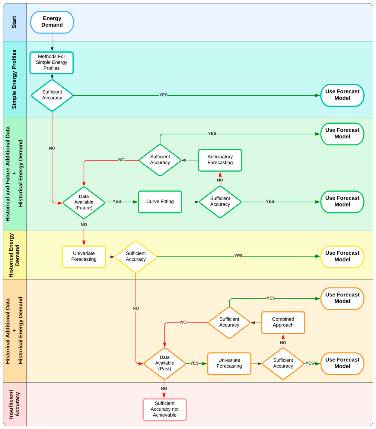
Finally, based on the conclusions drawn from the first three points, the guideline shown in Figure 3 has been developed to enable industry partners and other researchers to easily select the appropriate forecasting method based on the available data. A detailed description of the guideline is provided in Section 4.

To present all the newly defined terms clearly and concisely, they are summarised in

Table 4. Definitions of the data availability categories and forecasting methods.

Data Availability Categories
Terminology	Definition
Historical energy demand	Only historical energy demand is available and no other information.
Historical additional data + Historical energy demand	In addition to historical energy demand, further historical data are available (e.g., production data, weather forecast, shift plans etc.).
Historical and future additional data + Historical energy demand	In addition to historical energy demand, further data for the past and the future are available (e.g., production data, weather forecast, shift plans etc.).
Simple energy profiles	For simple energy profiles, only historical energy demand is available, as in the category “historical energy demand”. The difference here is the behaviour of the energy demand. If the energy demand has very simple and constant behaviour, special and easy-to-implement methods can be used. Therefore, these datasets have their own category.
Splitting energy demand based on time horizon	These are datasets that can be split based on time horizon (e.g., summer and winter, day and night, weekdays etc.). A specialised model can be developed for each part of the dataset with different methods.
Splitting energy demand based on consumer	These are datasets that can be split based on consumer (e.g., machines, buildings, shifts, lines etc.). A specialised model can be developed for each part of the dataset with different methods.
Forecasting Methods
Terminology	Definition
Univariate forecasting (historical energy demand)	This method predicts the energy demand based on its own history, patterns, and trends, without using additional data.
Univariate forecasting (historical energy demand and historical additional data)	This method predicts the energy demand based on its own history, patterns, and trends, using additional data from the past.
Combined approach	This approach is used if historical additional data and historical energy demand are available. It combines different methods to predict the energy demand. One method is used to predict the future additional data. This enables the use of methods that require historical and future additional data.
Curve fitting	With curve fitting, a function is created to predict the future energy demand. Therefore, future and past additional data are needed.
Anticipatory forecasting	Anticipatory forecasting methods require both future and past additional data, in parallel with historical energy consumption. These methods are commonly AI-based and can also be used when no additional data are available. However, the terminology anticipatory forecasting is implemented to emphasise that the additional data are used (past and future).
Methods for simple energy profiles	Methods that can be used for simple energy profiles (linear regression, polynomial regression, moving average, synthetic load profiles etc.).

.

4. Guideline for Developing Time Series Forecasting Models to Predict Industrial Energy Demand

This section describes the guideline for developing time series forecasting models to predict industrial energy demand. Figure 3 shows the entire process of the guideline. The guideline is based on categorising the data availability according to Figure 1. Each process step is described in detail in a separate section:

• Start
• Simple energy profiles
• Historical and future additional data
• Only historical energy demand data
• Historical additional data
• Insufficient accuracy

Step 1: Starts in Section 4.1, which explains the preparation for the development of the forecast model. Steps 2–6 (Section 4.2, Section 4.3, Section 4.4, Section 4.5 and Section 4.6): Explain when the different methods are applied and under which conditions. The process flow shown in Figure 3 must be followed. For each process step, an example from the analysed industrial projects is given. Furthermore, Table 5, Table 6, Table 7, Table 8, Table 9 and Table 10 present the characteristics for each process step.

The guideline is structured so that the methods that require the least effort to create and maintain are described at the beginning. The further the guideline progresses, the more complex and elaborate the methods become, and the corresponding expertise is required to apply the methods.

In addition, Step 7 (Section 4.7) is added to the guideline. Since the model needs to be updated and maintained and can be improved with new data, it is advisable to implement a monitoring system. A monitoring system ensures a reliable and stable operation of the forecast model. Thus, changes over time and new influences on the energy demand (implementation of new machines, changes in production, growth of the company, etc.) can be considered in the forecasting model. Furthermore, the monitoring system implements a continuous improvement process. As data collection will continue after the implementation of the forecasting model. In Step 7, it is described how these new data can be considered to improve the accuracy of the model.

Figure 3. Core guideline flow chart for developing time series forecasting models to predict industrial energy demand.

Figure 3. Core guideline flow chart for developing time series forecasting models to predict industrial energy demand.

4.1. Start

When starting with the guideline, the energy demand for which a forecast model needs to be created must be selected. This can be an individual unit, a group of several units or the entire company’s overall energy demand and can comprise different energy sources (e.g., electricity, heat, cooling, compressed air, etc.). At least a time-resolved profile from the analysed energy demand from the past is needed to develop a forecast model. If the energy demand of an entire plant is to be forecast, it is best to consider the company’s total energy demand and subdivide it according to the individual energy sources.

4.1.1. Splitting the Energy Demand Based on the Time Horizon

Splitting the data and creating a separate model for each segment can be helpful when creating a forecast model. In contrast to the splitting in Section 4.6.2, the data are split over time. If, for example, the behaviour of the energy demand differs significantly between weekdays and weekends, or between summer and winter, it can be helpful to divide the energy demand into these segments and create a separate model for each segment. For example, the following subdivisions were made for the forecast of heat demand:

• Weekday summer
• Weekday winter
• Weekday transitional period
• Saturday
• Sunday and public holidays

A separate forecast model was created for each segment. This made it possible to achieve higher accuracy in project 1 than with a single model for the entire period. Li et al. [8] also show that different models are preferable depending on the season (winter or summer).

4.1.2. Defining the Required Accuracy

Before starting with the selection of forecasting methods, it is necessary to determine what accuracy should be achieved with the forecasting methods. This depends on what the forecast is used for. One possibility is to improve existing forecasts. Then it is sufficient for the new forecasting methods if their accuracy is better than that of the current forecasting methods. The other possibility is that new methods are introduced for which a forecast is necessary (e.g., an optimisation method to minimise energy demand). In this case, the new method places certain requirements on the accuracy of the forecast. These form the basis for the minimum accuracy that the forecast must achieve. It is difficult to make a general statement as to when sufficient accuracy has been achieved. This depends not only on the sector and size of the industrial company but also on the current state of development of the company, the experience of the employees, the behaviour of the energy demand, the methods for which the forecast is to be used and the data availability and quality. Hence, it is not possible to make a general estimation of the accuracy for a specific method and research in this field is also lagging. Therefore, the required accuracy must be defined by the company itself.

4.2. Simple Energy Profiles

The first step is to analyse the selected energy demand in general to determine its complexity. There are three cases in which it makes sense to predict the energy consumption with simple profiles:

• Simple behaviour
• Low share of total energy demand
• Dead end

The last two points (low share of total energy demand and dead end) occur if no suitable forecast model is established when the guideline’s end is reached.

4.2.1. Simple Behaviour

If the analysed energy demand at the outset shows a clear trend or a recognisable pattern, the simplest possible methods should be used first for the forecast. If one of these methods achieves the desired accuracy, it is used for the forecast. If the desired accuracy is not achieved or none of the methods are applicable, continue with the next step in the guideline.

4.2.2. Low Share of Total Energy Demand

Section 4.6.2 describes how it is sometimes necessary to subdivide the analysed energy demand to achieve higher accuracy. If only a part of the original energy demand is analysed in the guideline, the share of that part of the original energy demand must be considered.

It is not expedient to use complex methods to achieve high accuracy for energy demands that only contribute a small percentage to the original energy demand. For example, assuming that the share of the analysed energy demand is only 5% of the original energy demand and the accuracy of the forecasting method is +/− 50%, that results in a fluctuation in the initially considered energy demand of only +/− 2.5%. It is, therefore, sufficient to use simple forecasting methods for energy demands that only contribute a small share to the overall forecast. This reduces the effort required to create and maintain the forecast models. Of course, the suitability of this approach must be verified individually for each case.

If the desired accuracy of the forecasting model is achieved, considering the share of the original energy demand, the developed forecasting model is used. If the accuracy is insufficient, continue with the next step of the guideline.

4.2.3. Dead End

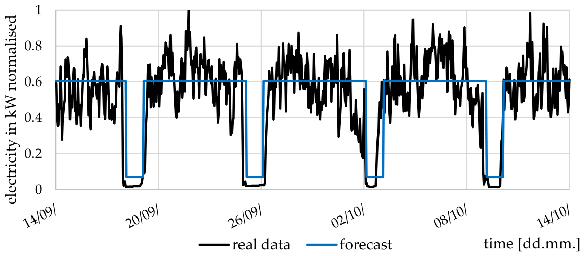
Sometimes, it is not possible to find a forecast model with sufficient accuracy (see Section 4.6.3). In this case, it is best to predict this energy demand as simply as possible. For example, the energy demand shown in Figure 4 fluctuates significantly. It is not possible to determine when the peaks occur without additional data. Further investigation is needed to understand this behaviour. Therefore, the average value was assumed for this energy consumption until more information about this production process could be determined.

4.2.4. Methods for Forecasting Simple Energy Profiles

Basic methods such as linear regression or moving average are used for the simple energy profiles. Further basic methods can be found in Abraham et al. [10] and Box et al. [11]. An overview of the characteristics of simple energy profiles is provided in Table 5.

Table 5. Overview of the forecast with methods for simple energy profiles.

Scope of application	– Energy demand with simple behaviour – Unpredictable energy demand (e.g., due to lack of information, energy behaviour, etc.)
Requirements	– Energy demand data from the past – Simple behaviour of the energy demand
Advantages	– Fast and simple implementation – Low maintenance effort – No special equipment or programmes necessary (but some are practical to support the user and reduce the workload) – No special knowledge is needed, because the methods are simple – Easily understandable models
Disadvantages	– To achieve high accuracy, simple behaviour (constant, repeating, low fluctuation) of the energy demand is essential
Methods	Linear regression, polynomial regression, moving average, synthetic load profiles, etc.
Literature	[10,11,12]

Table 5. Overview of the forecast with methods for simple energy profiles.

Scope of application	– Energy demand with simple behaviour – Unpredictable energy demand (e.g., due to lack of information, energy behaviour, etc.)
Requirements	– Energy demand data from the past – Simple behaviour of the energy demand
Advantages	– Fast and simple implementation – Low maintenance effort – No special equipment or programmes necessary (but some are practical to support the user and reduce the workload) – No special knowledge is needed, because the methods are simple – Easily understandable models
Disadvantages	– To achieve high accuracy, simple behaviour (constant, repeating, low fluctuation) of the energy demand is essential
Methods	Linear regression, polynomial regression, moving average, synthetic load profiles, etc.
Literature	[10,11,12]

Example:

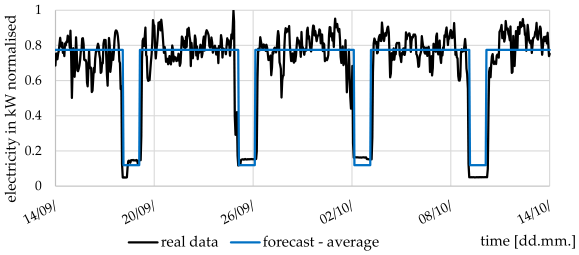
Figure 5 shows how to generate a forecast for a time series by averaging. A time series of eight weeks was analysed. The working days and the weekends were separated, and the mean value was calculated for the two categories. Figure 5 only shows a part of the eight weeks.

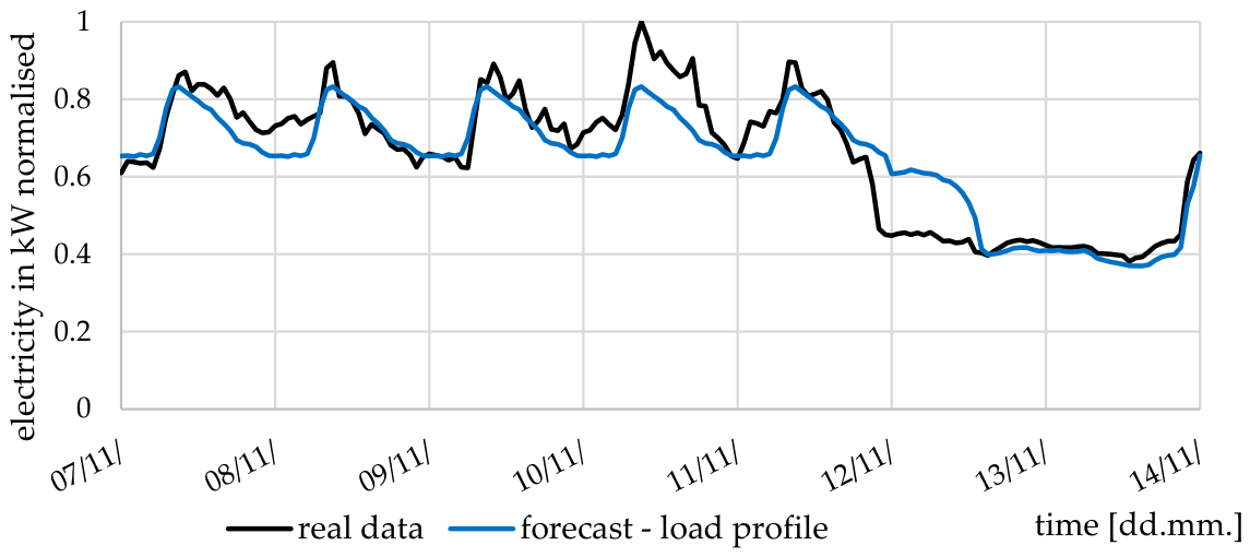
Synthetic load profiles are another option for creating a simple forecast model. These are particularly suitable if the behaviour of the time series is repetitive and characteristic. In Figure 6, a synthetic load profile is created for one day from a time series of eight weeks. Figure 6 shows the synthetic load profile compared to the real energy demand for one week. The load profile for one week is represented by the same five profiles for the working days from Monday to Friday and a separate profile for Saturday and Sunday. Every week, the load profile looks the same. The tool Visplore [24] is well-suited for creating synthetic load profiles.

4.3. Historical and Future Additional Data

If it is impossible to forecast energy demand using simple energy profiles, the next options are curve fitting and anticipatory forecasting. These forecasting methods require historical and future additional data (see Section 1 Introduction) that influence the energy demand to be forecast. If such additional data are known, they can improve the accuracy of the forecast models. If several datasets are considered as additional data, those datasets that significantly influence the energy demand should be used. Datasets without influence on energy demand should not be used, making it more challenging to create the forecast models. Correlation analyses are suitable for the selection of relevant input parameters. Further information on correlation analyses can be found in Cohen et al. [25] and Rönz et al. [26]. Visplore and Excel are suitable software tools for an initial quick check of the correlation, although many other tools, such as Python and MATLAB, are available. The choice is limited by the tools provided by the company and the knowledge of the creator of the forecast model. If no additional data are available for the future, proceed to the next step of the guideline.

When creating forecasting models with known data from the future, the first step is to try to develop the forecasting models using curve fitting. Anticipatory forecasting methods should be used only if this does not achieve the required accuracy. Anticipatory forecasting methods are more complex to develop than curve fitting and are particularly suitable for complex systems where the curve fitting method is no longer sufficient. Approaches from machine learning are mainly used for anticipatory forecasting.

4.3.1. Curve Fitting

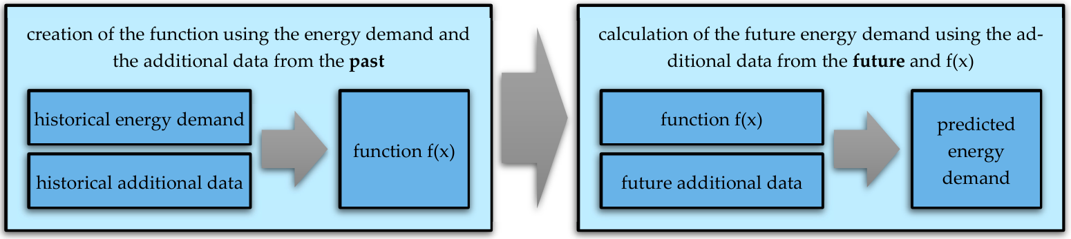
Curve fitting is about finding a function to calculate the energy demand from the available additional data. The function is created based on the data from the past (historical energy demand + historical additional data). Figure 7 shows the entire process from creating the curve fitting function to predicting the future energy demand. The created function reflects the relationship between the additional data and the energy demand. If additional data are available in the future, the future energy demand can be calculated using the developed function.

The function can be created in two ways using curve fitting. The first option is to create the entire function, meaning that the function type (linear, quadratic, etc.) and the corresponding coefficients are determined during the workflow. This can be achieved with the support of programmes such as Visplore. However, these have a disadvantage in that they are limited in terms of the function type. Visplore, for example, can only consider polynomial functions up to the fourth degree, not higher-order polynomial, exponential or sine functions. The other option is that the function type is specified, and only the coefficients are calculated. This has the advantage that any function can be investigated. However, it has the disadvantage that the different function types must be configured manually. For example, the Python package SciPy [12] offers curve fitting in this way.

The characteristics of curve fitting are summarised in Table 6.

Table 6. Overview of the forecast with curve fitting.

Scope of application	– Curve fitting is used when additional data from the past and the future are available and have a favourable correlation with the energy demand – It is an advantage if a good knowledge of the processes is available, as the correlations between the additional data and the energy demand can be determined more easily
Requirements	– Energy demand data from the past – Additional data from the past and the future – Correlation between additional data and energy demand
Advantages	– With a good correlation between additional data and energy demand, high accuracy is easy to reach – After the determination of the forecast model, it is easy to implement it in production as the outcome is a formula where the additional data from the future must be inserted to calculate the future energy demand – Simple maintenance of the forecast model—for an update of the model, only the formula has to be changed
Disadvantages	– To achieve a high level of accuracy, there must be sufficient correlation between the additional data and the energy demand – The prediction of the energy demand cannot have a higher accuracy than the prediction of the additional data from the future – A high level of knowledge is needed for interpreting the data and detecting the relation between energy demand and the additional data – Preliminary evaluation is needed for detecting the relation between energy demand and the additional data (e.g., correlation matrix, fast Fourier transformation, etc.)
Methods	Curve fitting and regression methods
Literature	[12,13]

Table 6. Overview of the forecast with curve fitting.

Scope of application	– Curve fitting is used when additional data from the past and the future are available and have a favourable correlation with the energy demand – It is an advantage if a good knowledge of the processes is available, as the correlations between the additional data and the energy demand can be determined more easily
Requirements	– Energy demand data from the past – Additional data from the past and the future – Correlation between additional data and energy demand
Advantages	– With a good correlation between additional data and energy demand, high accuracy is easy to reach – After the determination of the forecast model, it is easy to implement it in production as the outcome is a formula where the additional data from the future must be inserted to calculate the future energy demand – Simple maintenance of the forecast model—for an update of the model, only the formula has to be changed
Disadvantages	– To achieve a high level of accuracy, there must be sufficient correlation between the additional data and the energy demand – The prediction of the energy demand cannot have a higher accuracy than the prediction of the additional data from the future – A high level of knowledge is needed for interpreting the data and detecting the relation between energy demand and the additional data – Preliminary evaluation is needed for detecting the relation between energy demand and the additional data (e.g., correlation matrix, fast Fourier transformation, etc.)
Methods	Curve fitting and regression methods
Literature	[12,13]

Example:

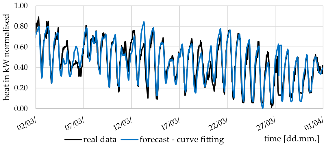
Among the analysed use cases, curve fitting was particularly suitable for forecasting the heat demand. Additional data on outdoor temperature and humidity were available. The data for these two datasets and the heat demand were available for one year. These data made it easy to visualise the relationship between the datasets and create formulas that could be used to calculate the heat demand. As the heat demand shows seasonal periodicity and differs significantly throughout the week, the dataset was split into different segments. For each segment, a corresponding fit function needs to be created, as subdividing the data increases the accuracy of the forecast (as already discussed in Section 4.1.1). The formula for calculating the heat demand (h_d) on all working days in winter is given here as an example:

$$h_d=1618.06+2.22\times h+0.00212\times t^4-88.58\times t$$

(1)

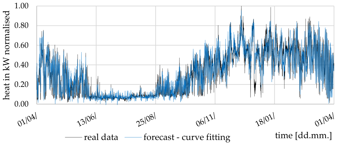
In Formula (1), only the outside temperature (t) and the hour of the day (h: integer values from 1 to 24) are needed. For some of the other segments, humidity is also required to achieve satisfactory accuracy. Figure 8 and Figure 9 show the comparison between the real heat demand and the calculated heat demand for one year and a section of 30 days. The curve fitting model reaches a coefficient of determination of 0.898. It should be noted that these calculations assumed that the outside temperature and the humidity were predicted correctly. This means that uncertainty in terms of the outdoor temperature and humidity forecast was not considered.

4.3.2. Anticipatory Forecasting

As already mentioned, anticipatory forecasting mainly uses machine learning approaches. Therefore, proper data preparation is important. Inaccurate data or data with outliers make it challenging to create a forecast model in a sufficient manner. These methods have the advantage compared to curve fitting that not only the correlation between energy demand and additional data is considered; patterns in the history (e.g., chart characteristics, seasonal influences, etc.) are also considered with anticipatory forecasting methods. All the advantages and disadvantages of the anticipatory forecasting and its characteristics are summarised in Table 7.

In the analysed use cases, neural networks, especially long short-term memory (LSTM) neural networks, have proved to be particularly suitable for time series forecasting. Further information on neural networks can be found in Legaard et al. [16] and Auffarth et al. [14]. Kulkarni et al. [15] provide a general overview of methods for developing forecasting models using machine learning.

Table 7. Overview of the forecast with anticipatory forecasting.

Scope of application	– Anticipatory forecasting is used when additional data from the past and the future are available and have a favourable correlation with the energy demand – Especially when the correlation between energy demand and additional data is hard to determine anticipatory forecasting can increase the accuracy compared to curve fitting – Anticipatory forecasting should only be used when the required accuracy cannot be achieved with curve fitting or the relation between energy demand and additional data is too complex to handle
Requirements	– Energy demand data from the past – Additional data from the past and the future – Correlation between additional data and energy demand
Advantages	– With a good correlation between additional data and energy demand, high accuracy can be reached – Possibility to improve during application—with new data, the model can improve itself and increase accuracy (lower maintenance is needed) – Relations between energy demand and additional data can be determined that are difficult to detect with other methods – No preliminary evaluation of the data is needed – Patterns in the history are also considered
Disadvantages	– To achieve a high level of accuracy, there must be sufficient correlation between the additional data and energy demand – The prediction of the energy demand cannot have a higher accuracy than the prediction of the additional data from the future – A high level of expertise in machine learning is required – Special hardware and software are needed – A maintenance strategy is needed
Methods	Machine learning and other AI methods
Literature	[14,15,16]

Table 7. Overview of the forecast with anticipatory forecasting.

Scope of application	– Anticipatory forecasting is used when additional data from the past and the future are available and have a favourable correlation with the energy demand – Especially when the correlation between energy demand and additional data is hard to determine anticipatory forecasting can increase the accuracy compared to curve fitting – Anticipatory forecasting should only be used when the required accuracy cannot be achieved with curve fitting or the relation between energy demand and additional data is too complex to handle
Requirements	– Energy demand data from the past – Additional data from the past and the future – Correlation between additional data and energy demand
Advantages	– With a good correlation between additional data and energy demand, high accuracy can be reached – Possibility to improve during application—with new data, the model can improve itself and increase accuracy (lower maintenance is needed) – Relations between energy demand and additional data can be determined that are difficult to detect with other methods – No preliminary evaluation of the data is needed – Patterns in the history are also considered
Disadvantages	– To achieve a high level of accuracy, there must be sufficient correlation between the additional data and energy demand – The prediction of the energy demand cannot have a higher accuracy than the prediction of the additional data from the future – A high level of expertise in machine learning is required – Special hardware and software are needed – A maintenance strategy is needed
Methods	Machine learning and other AI methods
Literature	[14,15,16]

Example:

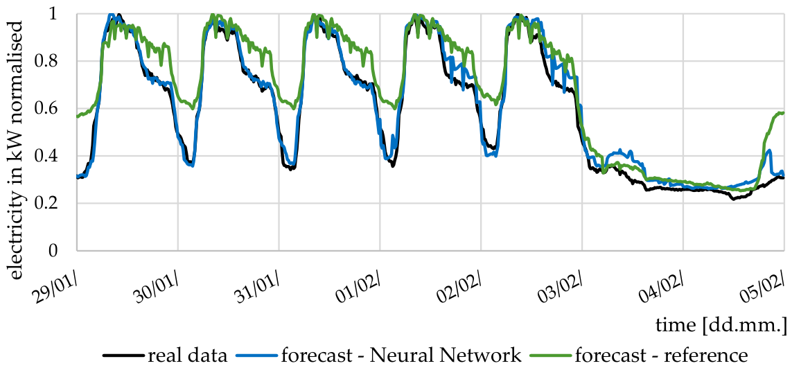
A forecasting model based on anticipatory forecasting was created for an automotive manufacturer. In addition to the energy demand from the past, production data such as shift plans and manufactured products are available. The production data are provided for both the past and the future, as they can be derived from the planned production programme. A neural network was trained using data from the past (data of one year) and subsequently tested in operation (for half a year). The trained neural network was used to forecast the energy demand for one week and then compared with the real data. Compared to the previously used forecasting method of the company (reference model), it was possible to improve the coefficient of determination from 0.91 to 0.98. Figure 10 compares the forecasts of the reference model, the neural network, and the real energy demand for one week. The improvements are achieved because the reference model does not consider the production data.

4.4. Only Historical Energy Demand Data

Univariate forecasting methods can be used if no additional data are available for the forecast and only the past energy demand is available. Due to the dependence on historical data, these approaches can be classified as data-driven (e.g., support vector machines, deep learning, machine learning, etc.) and mathematically describable relationships (including thermodynamic laws and basic laws of physics and chemistry) [7]. They can be derived based on the pattern of the historical energy demand. In comparison to the simple energy profiles, data-driven approaches are used in this process step of the guideline. Forecast models can be derived based on the past behaviour of the energy demand. The more irregular and random the behaviour of energy demand in the past, the more difficult it is to develop a reliable forecasting model using this methodology. Bourdeau et al. [17], Palma et al. [18], Vagropoulos et al. [19] and Makridakis et al. [7] have analysed and compared different methods for this purpose. Some of the methods mentioned in Section 4.3 are also used within the investigated use cases. Table 8 discusses univariate forecasting when it is only used with energy data from the past (for the characteristics which also include historical additional data, consider Table 9).

Table 8. Overview of the forecast with univariate forecasting (only historical energy demand available).

Scope of application	– Univariate forecasting is used when there are only historical energy demand data available
Requirements	– Energy demand data from the past
Advantages	– No additional data are needed—forecasts are possible only using the energy demand data from the past – Some methods of univariate forecasting can also consider additional data from the past (see Section 4.5.1)
Disadvantages	– Repeating behaviour of the energy demand is needed – If the energy demand depends on parameters other than time, such as temperature, production programme, etc., a forecast with high accuracy is difficult to achieve (no external influences considered) – Regular manual maintenance of the forecast model is needed (automated maintenance difficult to implement) – A high level of knowledge is needed to choose the right method—depending on the data, some methods are preferable to others—usually the different methods have to be tested to find the right one for the specific case – Special software and hardware can reduce the effort needed to establish and evaluate the forecasting models
Methods	Statistical methods (ARIMA, SARIMA, exponential smoothing, etc.), machine learning (LSTM neural networks, support vector machines, etc.) and combinations of them
Literature	[7,17,18,19,20,21]

Table 8. Overview of the forecast with univariate forecasting (only historical energy demand available).

Scope of application	– Univariate forecasting is used when there are only historical energy demand data available
Requirements	– Energy demand data from the past
Advantages	– No additional data are needed—forecasts are possible only using the energy demand data from the past – Some methods of univariate forecasting can also consider additional data from the past (see Section 4.5.1)
Disadvantages	– Repeating behaviour of the energy demand is needed – If the energy demand depends on parameters other than time, such as temperature, production programme, etc., a forecast with high accuracy is difficult to achieve (no external influences considered) – Regular manual maintenance of the forecast model is needed (automated maintenance difficult to implement) – A high level of knowledge is needed to choose the right method—depending on the data, some methods are preferable to others—usually the different methods have to be tested to find the right one for the specific case – Special software and hardware can reduce the effort needed to establish and evaluate the forecasting models
Methods	Statistical methods (ARIMA, SARIMA, exponential smoothing, etc.), machine learning (LSTM neural networks, support vector machines, etc.) and combinations of them
Literature	[7,17,18,19,20,21]

Example:

As part of a research project, the energy demand of an electric arc furnace (EAF) had to be predicted. As knowledge about future process parameters is not available due to inherent process conditions during electro-steel making, Zawodnik et al. [19] developed ultra-short-term forecasts (max. time horizon: 1 h) of the temporally resolved energy demand using historical data on the energy demand. This was realised with an LSTM neural network.

Depending on the predicted time horizon, different accuracies are reached. For a time horizon of 45 min and a resolution of 1 min, a mean absolute percentage error (MAPE) of approximately 18.7% could be reached with this forecast model.

4.5. Historical Additional Data

If, in addition to historical energy demand data, additional data are available as in Section 4.3, but only for the past and not for the future, univariate forecasting and a combined forecasting approach can be used. Whether the combined approach or the multivariate approach performs better depends on the specific characteristics of the time series data.

4.5.1. Univariate Forecasting (With Historical Additional Data)

As already mentioned in Section 4.4, the univariate forecasting approach can also be used to consider historical additional data. Wei [20], Kling et al. [21] and Mendis et al. [22] investigated univariate forecasting with historical additional data in detail. The methods and the procedure are the same as in Section 4.4. In contrast to the methods in Section 4.4, this method considers historical additional data. Table 9 presents the characteristics of the univariate forecasting with historical additional data.

Table 9. Overview of the forecast with univariate forecasting (historical energy demand and historical additional data).

Scope of application	– Univariate forecasting is primarily used when there are only historical energy demand data available, but can also be used if additional data from the past are available
Requirements	– Energy demand data from the past – Additional data from the past – Correlation between additional data and energy demand
Advantages	– Additional data from the past can be easily considered – With historical additional data, the accuracy of univariate forecasting can be improved
Disadvantages	– Repeating behaviour of the energy demand is needed – Regular manual maintenance of the forecast model is needed (automated maintenance difficult to implement) – A high level of knowledge is needed to choose the right method—depending on the data, some methods are preferable to others—usually the different methods have to be tested to find the right one for the specific case – Special software and hardware can reduce the effort needed to establish and evaluate the forecasting models
Methods	Statistical methods (ARIMA, SARIMA, exponential smoothing, etc.), machine learning (LSTM neural networks, support vector machines, etc.) and combinations of them
Literature	[7,17,18,19,20,21,22]

Table 9. Overview of the forecast with univariate forecasting (historical energy demand and historical additional data).

Scope of application	– Univariate forecasting is primarily used when there are only historical energy demand data available, but can also be used if additional data from the past are available
Requirements	– Energy demand data from the past – Additional data from the past – Correlation between additional data and energy demand
Advantages	– Additional data from the past can be easily considered – With historical additional data, the accuracy of univariate forecasting can be improved
Disadvantages	– Repeating behaviour of the energy demand is needed – Regular manual maintenance of the forecast model is needed (automated maintenance difficult to implement) – A high level of knowledge is needed to choose the right method—depending on the data, some methods are preferable to others—usually the different methods have to be tested to find the right one for the specific case – Special software and hardware can reduce the effort needed to establish and evaluate the forecasting models
Methods	Statistical methods (ARIMA, SARIMA, exponential smoothing, etc.), machine learning (LSTM neural networks, support vector machines, etc.) and combinations of them
Literature	[7,17,18,19,20,21,22]

4.5.2. Combined Forecasting Approach

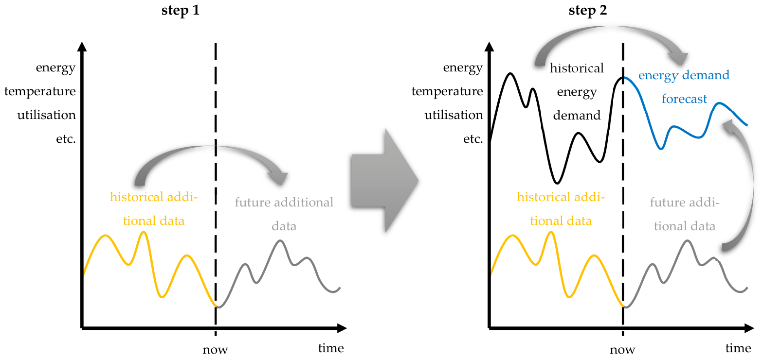
The combined approach is by far the most complex and should only be used if the other methods do not provide a suitable result. Moreover, as the input parameters used are also forecast, errors for the final forecast energy demand accumulate. The process of the combined forecasting approach is shown in Figure 11. Step 1 is to set up a model to predict the future additional data (marked grey in Figure 11) based on the historical additional data (marked yellow in Figure 11). Univariate forecasting methods from Section 4.4 are used for this, see Table 8. In Step 2, the model for predicting the energy demand is developed with the methods in Table 6 and Table 7 from Section 4.3. Therefore, follow the instructions in Section 4.3. As a result, two forecast models (one for the future additional data and one for the energy demand forecast) are developed. During application, first, the model from Step 1 must be executed to provide the future additional data for the forecast model to predict the energy demand.

The difference from the combined forecast approach to the method in Section 4.3 is that the future additional data are not available and a separate forecast model for the future additional data is needed.

Table 10. Overview of the forecast with the combined forecasting approach.

Scope of application	– The combined approach is used when the additional data are only available from the past and simple energy profiles or univariate forecasting cannot reach the required accuracy
Requirements	– Energy demand data from the past – Additional data from the past – Correlation between additional data and energy demand
Advantages	– Additional data can also be considered when they are only available from the past – Depending on the data, it is possible to achieve better accuracy compared to univariate forecasting – Same methods as for anticipatory forecasting and curve fitting can be used
Disadvantages	– Two models have to be developed and maintained—one for Step 1 and one for Step 2 – Accuracy depends on two models—if one model has low accuracy, the entire prediction has a low accuracy – A high level of expertise in the different methods is required – Special hardware and software are needed when machine learning methods are used
Methods	For Step 1: same as for univariate forecasting (statistical methods, e.g., ARIMA, SARIMA, exponential smoothing, etc., machine learning, e.g., LSTM neural networks, support vector machines, etc., and combinations of them) For Step 2: same as for curve fitting and anticipatory forecasting (curve fitting and regression methods—machine learning and other AI methods)
Literature	[3,7,12,13,14,15,16,17,18,19,23]

Table 10. Overview of the forecast with the combined forecasting approach.

Scope of application	– The combined approach is used when the additional data are only available from the past and simple energy profiles or univariate forecasting cannot reach the required accuracy
Requirements	– Energy demand data from the past – Additional data from the past – Correlation between additional data and energy demand
Advantages	– Additional data can also be considered when they are only available from the past – Depending on the data, it is possible to achieve better accuracy compared to univariate forecasting – Same methods as for anticipatory forecasting and curve fitting can be used
Disadvantages	– Two models have to be developed and maintained—one for Step 1 and one for Step 2 – Accuracy depends on two models—if one model has low accuracy, the entire prediction has a low accuracy – A high level of expertise in the different methods is required – Special hardware and software are needed when machine learning methods are used
Methods	For Step 1: same as for univariate forecasting (statistical methods, e.g., ARIMA, SARIMA, exponential smoothing, etc., machine learning, e.g., LSTM neural networks, support vector machines, etc., and combinations of them) For Step 2: same as for curve fitting and anticipatory forecasting (curve fitting and regression methods—machine learning and other AI methods)
Literature	[3,7,12,13,14,15,16,17,18,19,23]

Example:

In this example, the long-term energy demand of an EAF is to be forecast for a time horizon spanning up to 36 h [3]. Due to the statistically significant correlation between the required energy demand and the scrap mass used per charge, the scrap mass was predicted in the first step. Historical records of the scrap mass were available. Using a seasonal auto-regression integrated moving average (SARIMA) approach, the scrap masses of future batches could be reliably predicted (more information about SARIMA can be found in Palma et al. [18] and Vagropoulos et al. [19]). When calculating the future scrap masses, an rRSME value of less than 3.7% and an MAPE of less than 3.0% were achieved by Zawodnik et al. [3]. Studies have shown that SARIMA approaches are more accurate on average in predicting future scrap masses than machine learning methods or historical coincidence [7,23]. 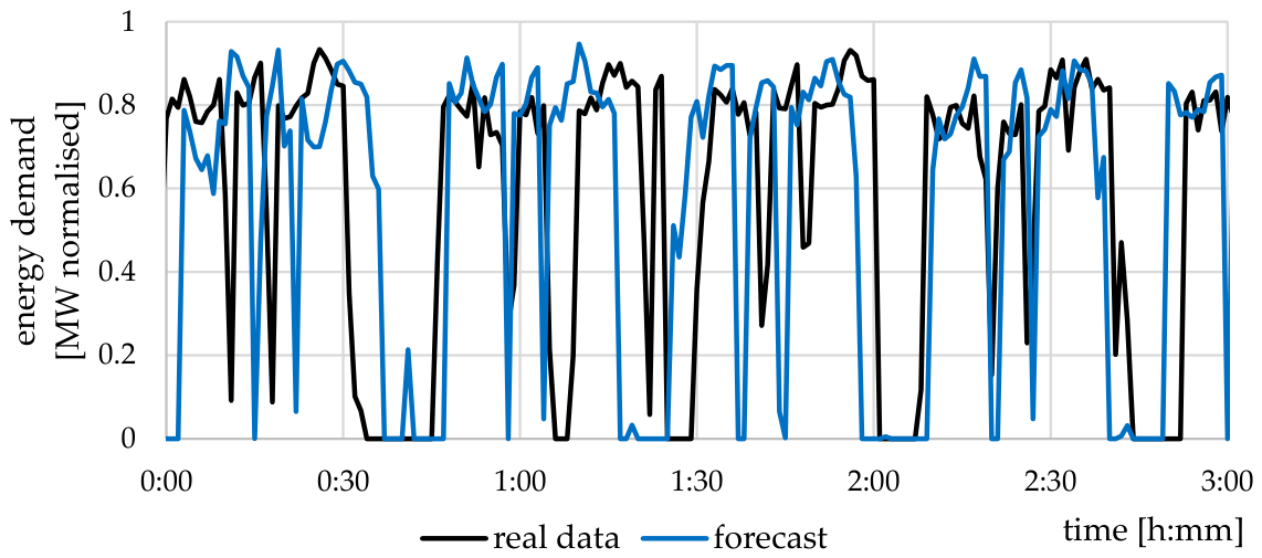However, methods based on SARIMA cannot process additional input parameter data, in contrast to approaches referenced in Section 4.3. The future energy consumption for one EAF batch can then be forecast based on the forecast scrap mass using the linear relationship to the required energy demand, followed by EAF operation phase-specific Markov chains to depict the stochastic operational behaviour of the EAF and generate the temporally resolved load profile. An example of the forecast and the actual data is shown in Figure 12. The forecast model achieves an average MAPE of 16.0% for a period of 36 h in a temporal resolution of one minute.

4.6. Insufficient Accuracy

If it is not possible to develop a forecast model with the methods mentioned above that achieves the required accuracy, the following options are available:

• Acquire new data
• Splitting of the energy demand
• Dead end

4.6.1. New Data

The energy demand often depends on external factors such as the outside temperature, maintenance intervals, production capacity utilisation, etc. If the required accuracy cannot be achieved, it is helpful to analyse which parameters are responsible for the fluctuations. The data of the newly determined influencing variables must then be extracted from the data management system, or if they are not yet recorded, appropriate measuring systems must be integrated. Once the new data have been prepared accordingly, continue developing the forecast model with the instructions in Section 4.3 or 4.5.

Example:

In one use case, the electricity demand of a production area with several plants fluctuated significantly and was therefore difficult to forecast. Additional data were required. It turned out that the share of machines in use, on standby or switched off influences the energy demand. After processing these data and integrating them into the development of the forecasting model, the MAPE could be reduced from 13.70% to 7.12%.

4.6.2. Splitting the Energy Demand Based on Consumer

For splitting, the analysed energy demand is subdivided more precisely. This requires additional measuring points to divide the energy demand between production areas or individual machines and systems, for example. This allows the behaviour of the individual areas to be analysed more accurately. Additional data on energy demand can presumably be identified more effectively than by analysing the overall energy demand.

Applying the Pareto principle [23] to divide into individual areas is helpful. In most cases, only a few systems are responsible for the largest share of the energy demand and several smaller ones only for a low share. In the steel industry, the arc furnace has the highest energy share, and in the pulp and paper industry, the drying process needs about 50% of the energy demand. In other industries and plants, too, a few machines, or one process, are commonly responsible for the main energy demand. Therefore, when creating the forecast models, the focus should be on the areas with a large share of energy demand. Smaller areas should be considered as simply as possible or can also be summarised.

When dividing into individual areas, it should be noted that the individual areas’ accuracy depends on the areas’ share in the originally considered energy demand. If the accuracy of areas with small shares is inferior, this can have a minor impact on the original energy demand.

It is possible that an area must be split again to create a forecast model. Multiple splitting can result in a tree structure. It is helpful to document this tree structure to maintain an overview of the splitting and the assignment of the individual forecast models.

4.6.3. Dead End

It may also be the case that the desired accuracy cannot be achieved, and neither splitting nor additional data can be conducted. If this is the case, selecting the simplest possible forecasting method from Section 4.2 is best.

If you reach the dead end, you must decide whether the forecasting model is sufficient for further use despite its inaccuracy. If it is insufficient, further investigations must be conducted to increase the accuracy. It may be necessary to install new measurement methods to generate additional data or to split the energy demand. Examining existing databases can also help find measurement points that have not yet been considered and influence the energy demand.

4.7. Controlling of the Models

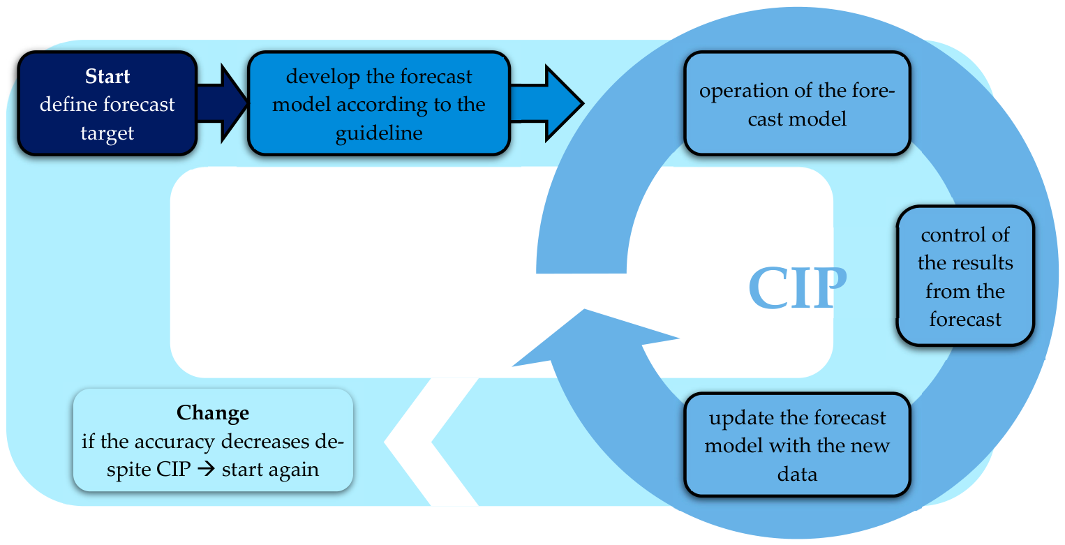
If a forecast model has been created and used, it must also be checked and updated during use. This involves comparing the forecast values with the real data. The accuracy of the forecast model may decrease over time. Changed processes, the installation of new machines and systems or behaviour patterns that were not considered when the forecast model was created can cause unwanted errors. The forecast model’s accuracy can be improved if the existing model is updated with new data. When calculating the mean value, as in Section 4.2, the mean value is recalculated with the current data; when using a neural network, it is retrained with the current data, etc. Ideally, the forecasting model is updated with the new data regularly. This works as a continuous improvement process (CIP) that can continually maintain or even increase the accuracy of the forecasting model. Sometimes, however, the accuracy of the forecast deteriorates despite updating with new data. If this happens, starting the process from the beginning and testing the different methods is necessary. This is referred to as a change. Figure 13 illustrates the workflow for the continuous improvement and the change process.

5. Discussion

Beginning with very simple methods and progressing to highly sophisticated methods, the guideline provides step-by-step instructions to determine the best solution for forecasting energy demand. If the accuracy is insufficient with the method used, follow the next step in the guideline to improve the accuracy. The accuracy depends strongly on the available data and the behaviour of the energy demand. Although it can be generally assumed that more data can improve the accuracy of the forecast, it does not guarantee that the accuracy improves. This depends on the quality of the data and whether all the significant parameters are added to the model. If a crucial parameter is missing or not predictable, the accuracy can only improve to the point possible without this parameter. It is also not possible to estimate the accuracy beforehand. The accuracy can only be determined after the forecast model has first been implemented and tested. As mentioned in Section 4.6, apart from adding new data, splitting the energy demand into parts (e.g., by room, machine or season) can help. It is then possible to identify where the lowest accuracy occurs and where new data or other methods are needed.

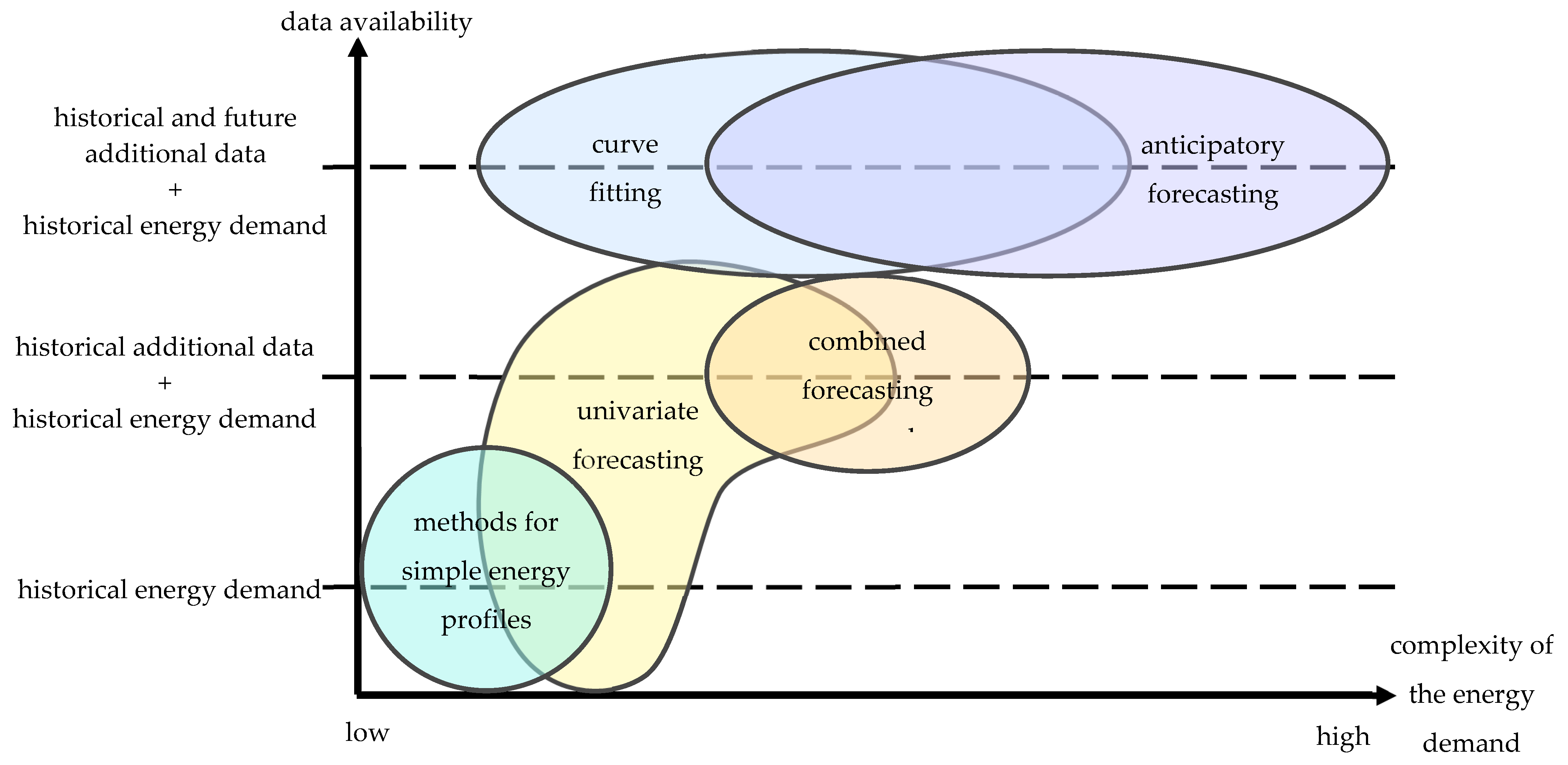
Depending on the data availability and the complexity of the energy demand (in this context, complexity refers to the influence of different parameters, such as temperature, production programme, raw material quality and human behaviour, on energy demand), different methods can be used. Every method mentioned in Section 3 and Section 4 can be assigned to the different levels of data availability and complexity, as presented in Figure 14. It shows where the different methods are most efficiently used.

Figure 14 has a blank top left corner for energy demands with low complexity and additional data availability. This does not mean that no other methods than simple energy profiles can be used (assuming the data are available), but there might be only a slight improvement of the accuracy due to the simple behaviour of the energy demand. Furthermore, the effort for implementation and maintenance is much higher than for simple energy profiles. Therefore, for energy demands with simple behaviour, more sophisticated forecasting models are not recommended as the effort is much higher and the improvement of the accuracy is negligible in most cases.

For energy demands with highly complex behaviour, forecasting becomes challenging. This is especially true if the data availability is low. If the energy demand depends heavily on additional data, it is not possible to set up a meaningful forecast model without any additional data. Hence, for complex energy demands, no methods are available when additional data is missing, as shown in Figure 14.

A prerequisite for using the guideline is that the data are available in one of the following three formats:

• Historical energy demand
• Historical energy demand + historical additional data
• Historical energy demand + historical and future additional data

Based on this information, the guideline leads you through the most suitable methods for establishing a deterministic model for forecasting energy demand. The guideline contains six different categories of methods (methods for simple energy profiles, univariate forecasting with historical energy demand, univariate forecasting with historical energy demand and historical additional data, combined forecasting approach, curve fitting and anticipatory forecasting). The literature listed here is a selection of the methods available. Listing all the possible methods would go beyond the scope of this study. Furthermore, research is currently increasing in this field (see Section 2) and new methods are constantly emerging that refine existing ones to achieve higher accuracy. Nevertheless, if a method can be assigned to one of the six method categories, it is covered by the guideline. The aim is for the literature provided in this paper to provide the user with a direction to follow. The literature used here consists of review papers and standard publications that outline the basic methods.

6. Conclusions

In contrast to existing research, this study categorises the methods used for forecasting the energy demand on the basis of the data availability. The available data determine which method can be used to forecast the energy demand. This classification is intended to make it easier for industrial companies to identify the right method. To make this as straightforward as possible for industrial companies, a dedicated guideline has also been developed.

The main purpose of the guideline is to provide a methodology to establish the best forecasting method according to the available data and the effort for setting up the forecast model. The methodology is demonstrated using different use cases and examples from the literature. This should ensure that the guideline covers all possible cases within the set restrictions. The current investigation of use cases and literature examples shows that the guideline is soundly developed, but comprehensive practical testing of its usability in industry is pending.

In this research, the focus is on deterministic forecasting methods. These methods are commonly used in industrial applications. Stochastic methods have negligible relevance for industrial companies. There are several reasons for the limited use of stochastic methods, such as a lack of data, no suitable installed tools, missing knowledge, and a poor cost-benefit ratio. Therefore, stochastic methods are not included in the guideline in this research. Nevertheless, in a holistic view of forecasting methods, stochastic methods should be included.

Another restriction concerning this guideline is the prediction horizon. This guideline is developed and tested for a prediction horizon from one hour to one week. No studies were conducted outside this time frame. Hence, further research is needed to determine whether the guideline can also be applied outside this range.

Predicting energy demand is a broad field of research. A wide variety of factors must be considered, ranging from the area of application (households, grid demand, industrial plants, transport, cities, etc.) to energy sources (electricity, natural gas, hydrogen, etc.) and the time horizon to be predicted (a few seconds, days, weeks or several years). There is currently no clear structure or procedure for finding the best method for forecasting energy demand in these different cases. Further research is needed to provide a structure for finding the best forecasting method for a given energy demand. The guideline developed in this paper aims to make a small contribution to this complex research topic.

References

- Islam, M.A.; Che, H.S.; Hasanuzzaman, M.; Rahim, N.A. Energy demand forecasting. In Energy for Sustainable Development; Elsevier: Amsterdam, The Netherlands, 2020; pp. 105–123. ISBN 9780128146453. [Google Scholar]
- Weigend, A.S. Time Series Prediction: Forecasting the Future and Understanding the Past; Routledge: Boulder, NV, USA, 2018; ISBN 9780429961199. [Google Scholar]
- Zawodnik, V.; Schwaiger, F.C.; Sorger, C.; Kienberger, T. Tackling Uncertainty: Forecasting the Energy Consumption and Demand of an Electric Arc Furnace with Limited Knowledge on Process Parameters. Energies 2024, 17, 1326. [Google Scholar] [CrossRef] [Scilit]
- Makridakis, S.G.; Wheelwright, S.C. Interactive Forecasting: Univariate and Multivariate Methods, 2nd ed.; Holden-Day: San Francisco, CA, USA, 1978; ISBN 9780816254163. [Google Scholar]
- Deb, C.; Zhang, F.; Yang, J.; Lee, S.E.; Shah, K.W. A review on time series forecasting techniques for building energy consumption. Renew. Sustain. Energy Rev. 2017, 74, 902–924. [Google Scholar] [CrossRef] [Scilit]
- Klyuev, R.V.; Morgoev, I.D.; Morgoeva, A.D.; Gavrina, O.A.; Martyushev, N.V.; Efremenkov, E.A.; Mengxu, Q. Methods of Forecasting Electric Energy Consumption: A Literature Review. Energies 2022, 15, 8919. [Google Scholar] [CrossRef] [Scilit]
- Makridakis, S.; Spiliotis, E.; Assimakopoulos, V.; Semenoglou, A.-A.; Mulder, G.; Nikolopoulos, K. Statistical, machine learning and deep learning forecasting methods: Comparisons and ways forward. J. Oper. Res. Soc. 2023, 74, 840–859. [Google Scholar] [CrossRef] [Scilit]
- Li, W.; Sui, W.; Cheng, L.; Ji, Y.; Guo, Y.; Zhu, J. Quantifying seasonal demand-side flexibility in residential air conditioning under diverse control strategies. Energy Build. 2026, 352, 116764. [Google Scholar] [CrossRef] [Scilit]
- Barker, J. Machine learning in M4: What makes a good unstructured model? Int. J. Forecast. 2020, 36, 150–155. [Google Scholar] [CrossRef] [Scilit]
- Abraham, B. Statistical Methods for Forecasting; Wiley: New York, NY, USA, 1983; ISBN 978-0-471-76987-3. [Google Scholar]
- Box, G.E.P.; Jenkins, G.M.; Reinsel, G.C.; Ljung, G.M. Time Series Analysis: Forecasting and Control, 5th ed.; Wiley: Hoboken, NJ, USA; EBSCO Industries: Hoboken, NJ, USA; Ipswich, MA, USA, 2016; ISBN 9781118674925. [Google Scholar]
- Vogel, J. Prognose von Zeitreihen; Springer Fachmedien Wiesbaden: Wiesbaden, Germany, 2015; ISBN 978-3-658-06836-3. [Google Scholar]
- Virtanen, P.; Gommers, R.; Oliphant, T.E.; Haberland, M.; Reddy, T.; Cournapeau, D.; Burovski, E.; Peterson, P.; Weckesser, W.; Bright, J.; et al. SciPy 1.0: Fundamental algorithms for scientific computing in Python. Nat. Methods 2020, 17, 261–272. [Google Scholar] [CrossRef] [Scilit] [PubMed]
- Auffarth, B. Machine Learning for Time-Series with Python: Forecast, Predict, and Detect Anomalies with State-of-the-art Machine Learning Methods; Packt Publishing Limited: Birmingham, UK, 2021; ISBN 9781801816106. [Google Scholar]
- Kulkarni, A.R.; Shivananda, A.; Kulkarni, A.; Krishnan, V.A. Time Series Algorithms Recipes: Implement Machine Learning and Deep Learning Techniques with Python, 1st ed.; Apress: New York, NY, USA; Imprint Apress: Berkeley, CA, USA, 2023; ISBN 9781484289778. [Google Scholar]
- Legaard, C.; Schranz, T.; Schweiger, G.; Drgoňa, J.; Falay, B.; Gomes, C.; Iosifidis, A.; Abkar, M.; Larsen, P. Constructing Neural Network Based Models for Simulating Dynamical Systems. ACM Comput. Surv. 2023, 55, 1–34. [Google Scholar] [CrossRef] [Scilit]
- Bourdeau, M.; Zhai, X.q.; Nefzaoui, E.; Guo, X.; Chatellier, P. Modeling and forecasting building energy consumption: A review of data-driven techniques. Sustain. Cities Soc. 2019, 48, 101533. [Google Scholar] [CrossRef] [Scilit]
- Palma, W. Time Series Analysis, 1st ed.; John Wiley & Sons Incorporated: Newark, NJ, USA, 2016; ISBN 9781118634349. [Google Scholar]
- Vagropoulos, S.I.; Chouliaras, G.I.; Kardakos, E.G.; Simoglou, C.K.; Bakirtzis, A.G. Comparison of SARIMAX, SARIMA, modified SARIMA and ANN-based models for short-term PV generation forecasting. In Proceedings of the 2016 IEEE International Energy Conference (ENERGYCON), Leuven, Belgium, 4–8 April 2016; IEEE: Piscataway, NJ, USA, 2016; pp. 1–6. ISBN 978-1-4673-8463-6. [Google Scholar]
- Wei, W.W.S. Multivariate Time Series Analysis and Applications; John Wiley & Sons: Hoboken, NJ, USA, 2019; ISBN 9781119502852. [Google Scholar]
- Kling, J.L.; Bessler, D.A. A comparison of multivariate forecasting procedures for economic time series. Int. J. Forecast. 1985, 1, 5–24. [Google Scholar] [CrossRef] [Scilit]
- Mendis, K.; Wickramasinghe, M.; Marasinghe, P. Multivariate Time Series Forecasting: A Review. In Proceedings of the CVIPPR 2024: 2024 2nd Asia Conference on Computer Vision, Image Processing and Pattern Recognition, Xiamen, China, 26–28 April 2024; ACM: New York, NY, USA, 2024; pp. 1–9. ISBN 9798400716607. [Google Scholar]
- Zawodnik, V. Prognosemodellierung des Energiebedarfs eines Elektrolichtbogenofens—Die Herausforderung im Umgang mit begrenztem Wissen. Wien, 16 February 2023. Available online: https://view.officeapps.live.com/op/view.aspx?src=https%3A%2F%2Fiewt2023.eeg.tuwien.ac.at%2Fdownload%2Fcontribution%2Fabstract%2F15%2F15_abstract_20221110_104721.docx&wdOrigin=BROWSELINK (accessed on 7 May 2026).
- Visplore. Visplore—Software for Visual Time Series Analysis. Available online: https://visplore.com/ (accessed on 19 April 2024).
- Cohen, J.; Cohen, P.; West, S.G.; Aiken, L.S. Applied Multiple Regression/Correlation Analysis for the Behavioral Sciences, 3rd ed.; Taylor and Francis: Mahwah, NJ, USA, 2003; ISBN 9781134800940. [Google Scholar]
- Rönz, B. Regressions- und Korrelationsanalyse: Grundlagen—Methoden—Beispiele; Springer Gabler. in Springer Fachmedien Wiesbaden GmbH: Wiesbaden, Germany, 1992; ISBN 9783322964960. [Google Scholar]