Measuring Peak Shaving Efficiency of an Energy Storage Device Under Load Uncertainty with Machine Learning-Based Forecasting Techniques

Abstract

Energy storage systems enhance grid efficiency by mitigating peak demand and balancing generation variability. This work addresses the challenge of achieving optimal peak shaving without prior knowledge of the actual load profile. To this end, we introduce the Forecast-Integrated Shortest Path (FISP) framework, which integrates load forecasting with the shortest-path optimization algorithm to determine optimal generation and storage strategies under forecast uncertainty. A penalty-based metric is proposed to quantify the deviation between forecast-driven and ideal operation, providing a unified measure of forecast-to-optimization performance. The proposed approach is validated using real load data from the European Network of Transmission System Operators for Electricity (ENTSO-E) and evaluated with two forecasting techniques—Long Short-Term Memory (LSTM) networks and Autoregressive Moving Average (ARMA) models. The results show that LSTM-based forecasts yield substantially lower penalties than ARMA, demonstrating that accurate prediction combined with intelligent storage control can significantly enhance operational reliability and peak-shaving performance.

1. Introduction

Modern power systems face persistent challenges arising from fluctuating load demands, peak load management, and the increasing integration of renewable energy sources. The ongoing transition to smarter, more sustainable grids requires innovative strategies to ensure efficient planning, control, and operation. In distribution networks, the growing penetration of renewable generation has introduced higher variability and bidirectional power flows between distribution and transmission systems [1].

Beyond technical reliability, economic efficiency has become equally critical. The high startup costs of thermal generation units underscore the importance of effective operational management [2]. Peak-demand charges and off-peak underutilization remain major issues in grid economics, motivating the adoption of strategies such as peak shaving and valley filling [3,4]. Energy storage systems play a central role in these strategies by enabling load shifting, balancing, and backup capacity. However, while renewable integration improves sustainability, its inherent intermittency and low system inertia necessitate the use of storage to maintain stability and cost-effectiveness [5,6].

Accurate load forecasting plays a vital role in optimizing power generation, reducing fuel consumption, and minimizing operational costs. However, forecasting uncertainty remains a major challenge for reliable grid management [5]. Traditional approaches rely on statistical models such as the Autoregressive Moving Average (ARMA) model [5,7], while more advanced techniques employ machine learning architectures, including artificial neural networks (ANNs) and long short-term memory (LSTM) networks, to better capture nonlinear and long-term dependencies in the data.

In parallel, numerous studies have focused on operational optimization and peak shaving strategies. Analytical approaches have been proposed for sizing and controlling energy storage systems based on historical load profiles [8], while smart grid control and market-based mechanisms have been developed to manage peaks through demand-side participation [1,9]. Other works highlight the use of aggregated battery systems and joint optimization frameworks for storage management under uncertainty [3,4].

A particularly relevant study is presented in [7], where the authors propose an analytical shortest-path algorithm to determine the minimum achievable generation peak based on the load profile and available storage capacity, while this method provides an elegant and computationally efficient framework for optimal storage utilization, it assumes perfect knowledge of the load profile—an assumption that rarely holds in real-world operation, where forecasts are inherently uncertain.

This gap motivates the present work, which aims to bridge the divide between load forecasting and generation optimization by integrating forecasted profiles directly into the shortest-path optimization framework. In doing so, we evaluate how forecasting uncertainty affects operational performance and introduce a quantitative penalty metric to measure the impact of forecast accuracy on optimal control decisions. Motivated by the aforementioned limitations of the Shortest Path algorithm—particularly its dependence on perfect knowledge of the load profile—this work builds upon those constraints to propose a unified framework that integrates load forecasting with operational optimization.

We introduce the Forecast-Integrated Shortest Path (FISP) framework, a numerical optimization approach that refines forecasted electricity loads while accounting for the characteristics and constraints of available energy storage systems. The proposed methodology bridges the gap between forecasting and control, enabling quantitative evaluation of how forecast uncertainty influences operational decisions. The main contributions of this work are summarized as follows:

• Optimal energy-storage management under uncertainty:
  We present a method for peak-shaving that integrates load-forecasting techniques with a shortest-path-based optimization algorithm. This formulation achieves optimal operation while mitigating the effects of forecast errors. In addition, we introduce a dedicated performance metric to evaluate the effectiveness of the proposed approach.
• Validation on real-world data:
  The framework is evaluated using data from the European Network of Transmission System Operators for Electricity (ENTSO-E) and compared across two forecasting models—the statistical ARMA model and the deep-learning-based LSTM network.
• Penalty-based evaluation metric:
  We define a novel penalty metric that quantifies the discrepancy between the optimal generation profile obtained from the actual load and that derived from the forecasted load, thereby providing a practical means to assess forecast-driven control performance.

2. Related Works

Accurate load forecasting has long been recognized as a cornerstone of reliable and efficient power system operation. Comprehensive surveys of forecasting methodologies [10,11] have detailed the evolution from statistical models, such as ARMA and ARIMA, to advanced deep-learning architectures including LSTM, GRU, and hybrid networks. These reviews underline the superior predictive capacity of neural models in capturing nonlinear consumption dynamics and temporal dependencies. However, they primarily assess forecast accuracy, without addressing how forecast uncertainty influences downstream operational decisions—a gap that motivates the present study.

Complementary analyses, such as [11], provide extensive performance comparisons of machine learning and deep learning models based on standard error metrics (MAE, RMSE, MAPE). While these benchmarks effectively quantify prediction accuracy, they do not extend to the operational layer, where forecast errors can propagate into suboptimal generation or storage scheduling. This distinction is crucial in practical grid management, where forecasting precision alone does not guarantee efficient operation.

Beyond pure forecasting studies, recent reviews have explored the integration of artificial intelligence into energy management systems and smart grid optimization [12]. These works highlight the growing use of LSTM and CNN models to manage the stochasticity of renewable generation and demand, and discuss how metaheuristic algorithms can enhance scheduling performance. Nevertheless, most of these frameworks focus on long-term coordination or heuristic optimization and do not explicitly quantify the operational impact of short-term forecast errors. The proposed Forecast-Integrated Shortest Path (FISP) framework complements this line of research by directly coupling load forecasting with an analytical optimization layer, and by introducing a penalty-based metric to systematically evaluate forecast-to-operation performance.

Recent advances in load forecasting have increasingly focused on adaptive and hybrid learning techniques to improve accuracy under dynamic grid conditions. Reference [13] introduced an adaptive online learning framework based on hidden Markov models for probabilistic load forecasting, effectively capturing uncertainty and concept drift in evolving consumption patterns. Building upon such adaptive principles, ref. [14] proposed a CNN-LSTM network optimized for multi head attention with particle swarms that integrates deep learning and evolutionary optimization to improve short-term load prediction accuracy, achieving mean absolute percentage errors below 2%. Similarly, ref. [15] developed DA-LSTM, a drift-adaptive recurrent neural framework that dynamically adjusts to shifting load behaviors, improving interval forecasts without predefined drift thresholds. Together, these studies highlight the growing role of adaptive and data-driven models in achieving robust and accurate load forecasting for modern smart-grid applications.

In parallel, optimization and energy management strategies for system with batteries have increasingly attracted attention. In the study [16], a polynomial-time algorithm is presented for the lossless battery charging problem by reformulating the mixed-integer linear programming (MILP) model as a shortest-path problem, allowing efficient and exact scheduling under ideal conditions ($\eta =1$). Building on the theme of optimization in energy storage management, ref. [17] propose a cycle-based control strategy combined with cluster-level power allocation optimized through particle swarm optimization (PSO), demonstrating improvements in capture and release rates, as well as an increase in capacity utilization from 75.1 % to 79.9% and a 3.7% reduction in energy losses for peak cleaning applications. Complementing these approaches, ref. [18] introduce an optimization-based control method that computes an optimal shave level from historical load data—augmented by statistical confidence modeling—to dynamically guide battery charge and discharge operations while accounting for the finite charging and discharge rates of real battery systems.

Recent research in energy systems increasingly leverages modern deep–learning architectures such as BiLSTM networks combined with multi-head self-attention mechanisms [19] and hybrid CNN-BiLSTM-attention models for battery state-of-charge estimation [20]. Such models are capable of capturing long-range temporal dependencies, nonlinear degradation patterns, and multi-variable correlations more effectively than classical recurrent networks. In parallel, advanced multi-objective optimization frameworks—such as deep reinforcement learning-based energy management strategies accounting for fuel-cell degradation and future terrain information—have demonstrated significant improvements in economic cost and component longevity [21].

These strands of work illustrate the rapid evolution of data-driven forecasting and multi-objective control in modern energy systems. In the present study, however, our goal is fundamentally different: to introduce and validate the Forecast-Integrated Shortest Path (FISP) framework, focusing on how forecast uncertainty interacts with the analytical shortest-path operator. Accordingly, we intentionally employ classical ARMA and standard LSTM models as baselines—not to exhaust the forecasting frontier, but to provide a clean evaluation of how any forecasting model (simple or advanced) propagates through the SP optimization layer. The advanced architectures above represent promising future extensions that can be seamlessly integrated into the FISP pipeline to further enhance forecast-to-operation consistency.

3. Technical Background

This section provides the theoretical foundations required to understand the proposed Forecast-Integrated Shortest Path (FISP) framework. We begin by reviewing the principles of peak shaving and the role of energy storage systems in modern power grids. Then, we describe the Shortest Path Algorithm, which forms the optimization core of the proposed method. Together, these concepts establish the technical basis for integrating load forecasting with operational optimization in subsequent sections.

3.1. Peak Shaving and Energy Storage Management

Energy storage technologies play a central role in enabling modern power systems to operate flexibly and efficiently. By absorbing surplus energy during periods of low demand and discharging it during peak hours, storage devices support key operational objectives such as load leveling, reserve provision, congestion relief, and peak shaving [6].

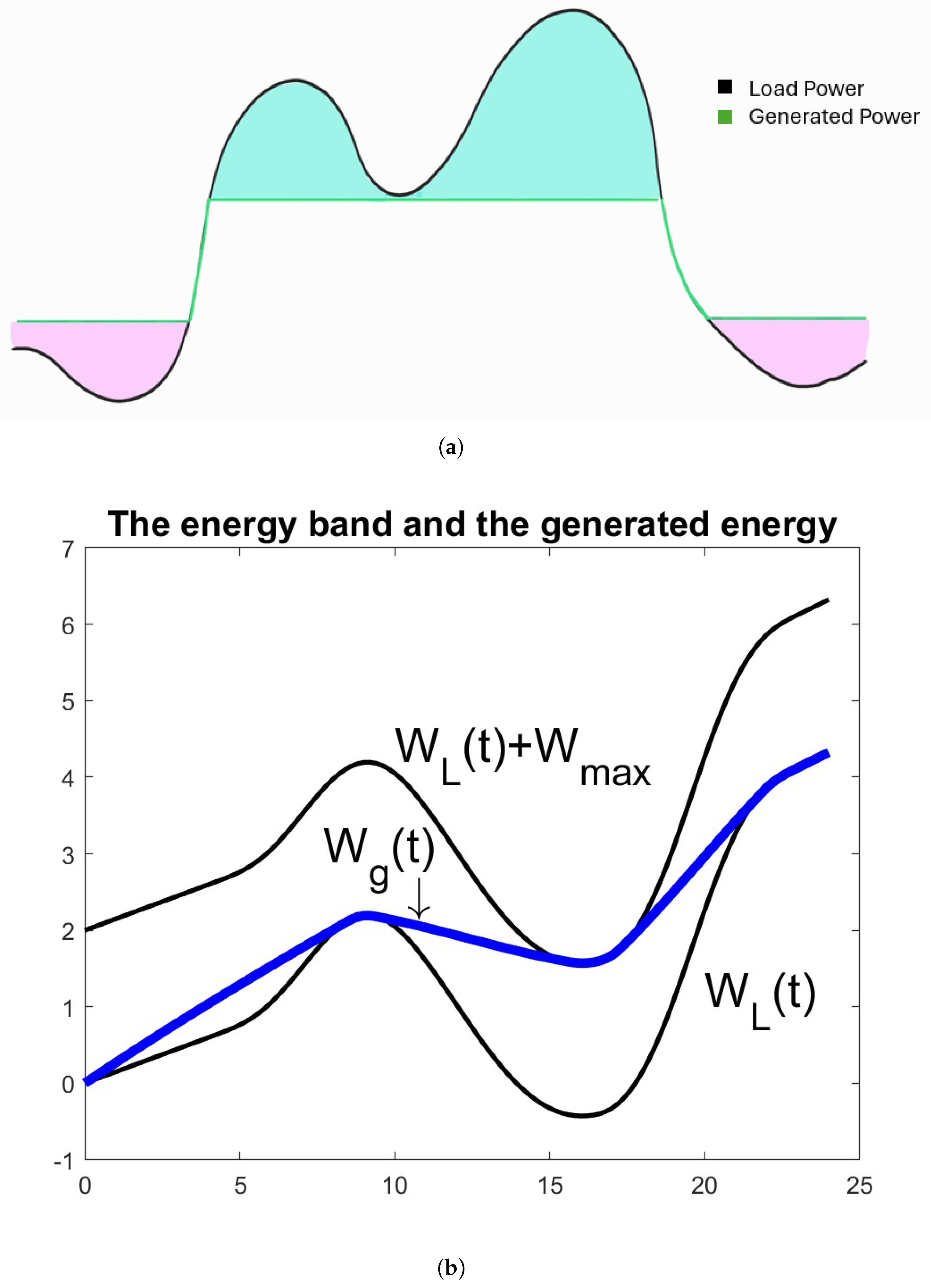
Peak shaving—illustrated in Figure 1a—mitigates extreme demand peaks by shifting energy temporally. This reduces stress on generation assets and transmission infrastructure, lowers operational costs, and reduces dependence on high-emission peaker plants, thereby contributing to a cleaner and more resilient grid [6,7]. Because storage interacts directly with the net load, the effectiveness of peak shaving depends not only on physical capacity but also on the controller’s ability to anticipate demand variations. This need becomes even more critical as renewable generation introduces additional variability and uncertainty into daily load profiles. Accurate short-term forecasting becomes essential: when the charging and discharging decisions are aligned with future load trajectories, storage can be deployed more efficiently, achieving deeper peak reductions with the same energy capacity. Conversely, forecast errors can lead to suboptimal use of storage—mis-timed charging, insufficient discharge during peaks, or unnecessary cycling—all of which reduce the operational benefit of the device.

These considerations motivate the integration of forecasting and optimization in a unified framework. The FISP approach developed in this work builds precisely on this principle: using predictive models to inform peak-shaving scheduling, enabling storage to achieve near-optimal performance even under uncertainty.

3.2. The Shortest-Path Algorithm

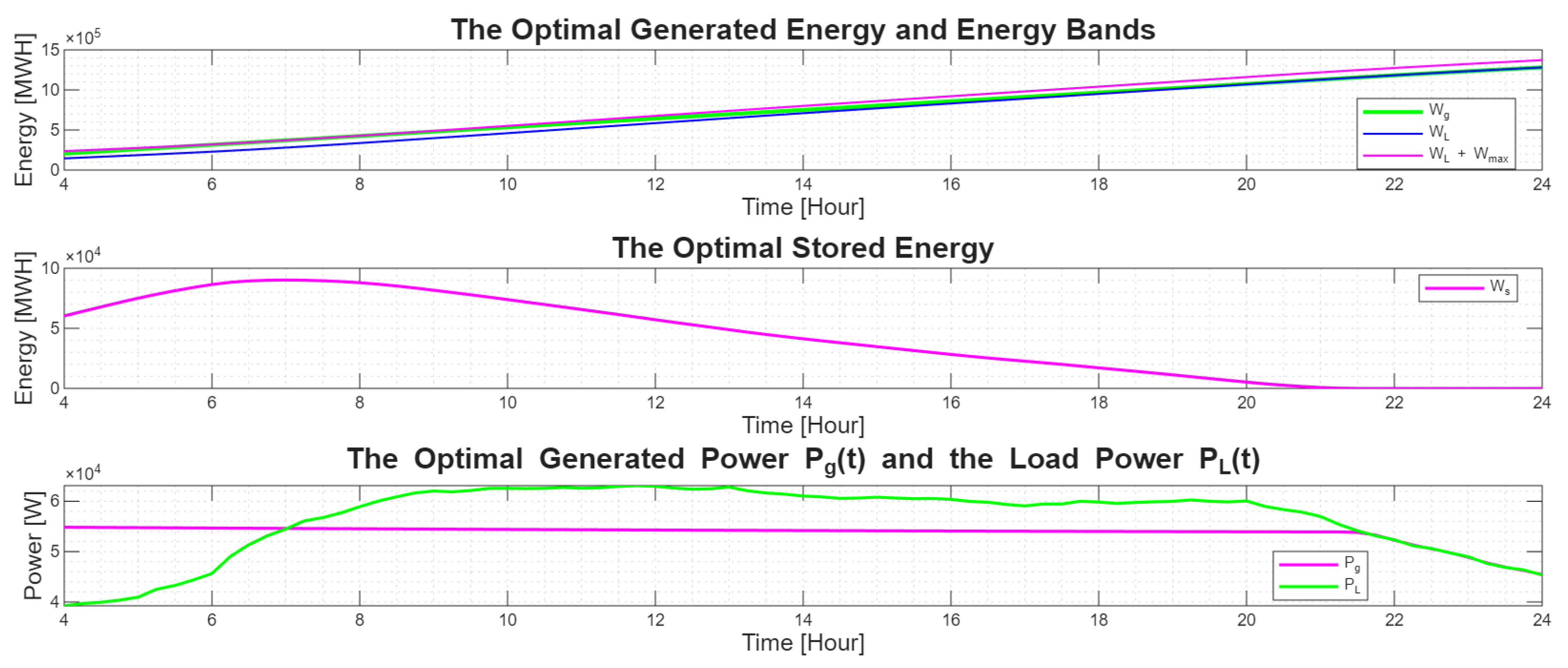
The Shortest-Path formulation used in this work follows the derivation of [7], where the peak-shaving problem is expressed in the energy domain. An example of the optimal generated power and stored energy trajectories obtained by applying the Shortest-Path algorithm to the actual load profile is illustrated in Figure 2.

3.2.1. Modeling Assumptions for the Shortest-Path

The classical Shortest-Path (SP) method relies on a set of structural assumptions that enable its analytical energy-band solution. For clarity and completeness, we list these assumptions explicitly:

• Ideal, lossless storage- the storage device is assumed to have no charging or discharging losses, no efficiency degradation, and no aging effects. Its energy

  $$W_s\left(t\right)=W_g\left(t\right)-W_L\left(t\right).$$

  (1)

  which leads directly to the energy-band constraint

  $$W_L\left(t\right)\le W_g\left(t\right)\le W_L\left(t\right)+W_{max}$$

  (2)
  This lossless model is required for the analytical SP formulation; introducing losses breaks the band structure and would require a different optimization method (e.g., MPC or DP).
• No charging/discharging power limits- the SP solution does not impose constraints on the instantaneous charging or discharging rate (no C-rate limits). The controller is therefore free to react instantaneously to load fluctuations within the energy-band boundaries. Incorporating realistic power limits again removes the closed-form SP solution and constitutes a separate research direction.
• Perfectly known storage capacity- the maximum reservoir size $W_{max}$ is treated as a deterministic, time-invariant parameter.
• Load profile drives the feasible region- the feasible generation trajectory is entirely determined by the load evolution and $W_{max}$. Any uncertainty in $P_L\left(t\right)$ therefore leads to deviations between the true and forecast-based optimal trajectories—precisely what the penalty metric measures.

These assumptions are standard in the analytical energy-band formulation of the Shortest-Path method and are necessary for deriving its closed-form solution. In this work, our primary objective is to address one of the two fundamental limitations of SP—its reliance on perfect prior load knowledge—by integrating forecasting models within the optimization loop. Extending the framework to include realistic efficiencies or C-rate limits requires replacing the analytical SP operator with a different optimization framework, and is therefore identified as an important direction for future work.

3.2.2. Energy Bands Theory

The generated power at time t, denoted $p_g\left(t\right)$, is fully controllable and may be supplied directly to the load or routed into storage. Its operational cost is modeled by a strictly convex, monotonically increasing function $F\left(p_g\left(t\right)\right)$, yielding the total cost

$$F_{\mathrm{tot}}={{\displaystyle \mathit{\int }}}_0^{T}F\left(p_g\left(t\right)\right)d\tau .$$

(3)

Under strict convexity, minimizing $F_{\mathrm{tot}}$ is equivalent to minimizing the peak value ${max}_t{p}_g\left(t\right)$.

The power balance at each instant is

$$p_s\left(t\right)=p_g\left(t\right)-p_L\left(t\right),$$

(4)

where $p_L\left(t\right)$ is the net load. To incorporate renewable generation, we define

$$p_L\left(t\right)=p_{\mathrm{load}}\left(t\right)-\left|p_{\mathrm{ren}}\left(t\right)\right|,$$

so that renewable contributions reduce the effective demand on the dispatchable generator.

Cumulative energies are given by

$$W_g\left(t\right)={{\displaystyle \mathit{\int }}}_0^t{p}_g\left(\tau \right)d\tau , W_L\left(t\right)={{\displaystyle \mathit{\int }}}_0^t{p}_L\left(\tau \right)d\tau , W_s\left(t\right)={{\displaystyle \mathit{\int }}}_0^t{p}_s\left(\tau \right)d\tau ,$$

(5)

with the storage capacity constraint

$$0\le W_s\left(t\right)\le W_{max}.$$

(6)

The analytical solution requires an ideal storage device, with no charging or discharging losses, satisfying (1) which transforms the storage constraint into the energy-band condition (2). Thus, $W_g\left(t\right)$ must remain within an upper and lower boundary defined entirely by the load and the storage capacity. The peak-shaving problem then becomes

$$\begin{array}{cc}\hfill \mathrm{minimize} & F_{\mathrm{tot}}={{\displaystyle \mathit{\int }}}_0^{T}F\left(p_g\left(t\right)\right)dt,\hfill \\ \hfill \mathrm{subject} \mathrm{to} & W_L\left(t\right)\le W_g\left(t\right)\le W_L\left(t\right)+W_{max}.\hfill \end{array}$$

(7)

Geometrically, the optimal generated-energy trajectory $W_g\left(t\right)$ is the shortest feasible path within the energy band. For large $W_{max}$, this path approaches a straight line whose slope equals the average net load; for small $W_{max}$, $W_g\left(t\right)$ is forced to follow $W_L\left(t\right)$ closely.

Following [7], consider cost functions of the form $F\left(p\right)={\left|p\right|}^m$. In the limit $m\to \infty$,

$$\underset{m\to \infty }{lim}{\left({{\displaystyle \mathit{\int }}}_0^T{\left|p_g\left(t\right)\right|}^{m}dt\right)}^{1/m}=\underset{t}{max}{p}_g\left(t\right).$$

As proved in [22], the shortest Euclidean path of $W_g\left(t\right)$ is precisely the one that minimizes $F_{\mathrm{tot}}$, linking the geometric interpretation directly to the analytical optimality condition. The trajectory $W_g\left(t\right)$ minimizing this limiting quantity is therefore the shortest feasible path within the energy band, and its derivative $p_g\left(t\right)$ achieves the minimal possible generation peak. These assumptions provide the theoretical foundation for the Shortest-Path method used in this study. They yield an analytical characterization of optimal peak-shaving behavior and offer a clear geometric interpretation that connects storage capacity, load variability, and the resulting generation strategy.

3.3. Load Forecasting

Load forecasting methods are generally divided into three main categories: statistical, artificial intelligence (AI), and hybrid approaches. Statistical models such as the Autoregressive Moving Average (ARMA) model capture linear temporal dependencies effectively but may struggle with nonlinear patterns in modern power demand [2,23]. In contrast, AI-based approaches such as artificial neural networks and recurrent neural networks (RNNs) can model complex and nonlinear relationships, though they require longer training times and may suffer from overfitting [2,23].

In this study, we employ two representative forecasting methods: the classical ARMA model and the deep-learning-based Long Short-Term Memory (LSTM) network. The ARMA $(p,q)$ model expresses the current load ${\widehat{P}}_t$ as a linear combination of past values and previous error terms:

$${\widehat{P}}_t=AR\left(p\right)+MA\left(q\right)=\mu +\sum _{i=1}^p{\phi }_i{P}_{t-i}+\sum _{i=1}^q{\theta }_i{\epsilon }_{t-i}+{\epsilon }_t.$$

(8)

where $\mu$ is the mean load, ${\phi }_i$ and ${\theta }_i$ denote the autoregressive and moving average coefficients, and ${\epsilon }_t$ represents white noise.

The LSTM network, a specialized type of RNN [24], overcomes the vanishing gradient problem of traditional recurrent models by introducing a gated memory structure that selectively retains long-term dependencies. This design enables LSTM models to capture both short- and long-range temporal correlations in load demand data [25,26]. Formally, the input $x_t$, previous cell state $c_{t-1}$, and hidden state $h_{t-1}$ define the operation of an LSTM cell. A detailed schematic illustration of the standard LSTM cell can be found in [24].

Both model outputs serve as inputs to the proposed optimization layer, allowing direct evaluation of how forecasting quality influences operational performance.

4. Proposed Framework—Forecast-Integrated Shortest Path (FISP)

4.1. System Model

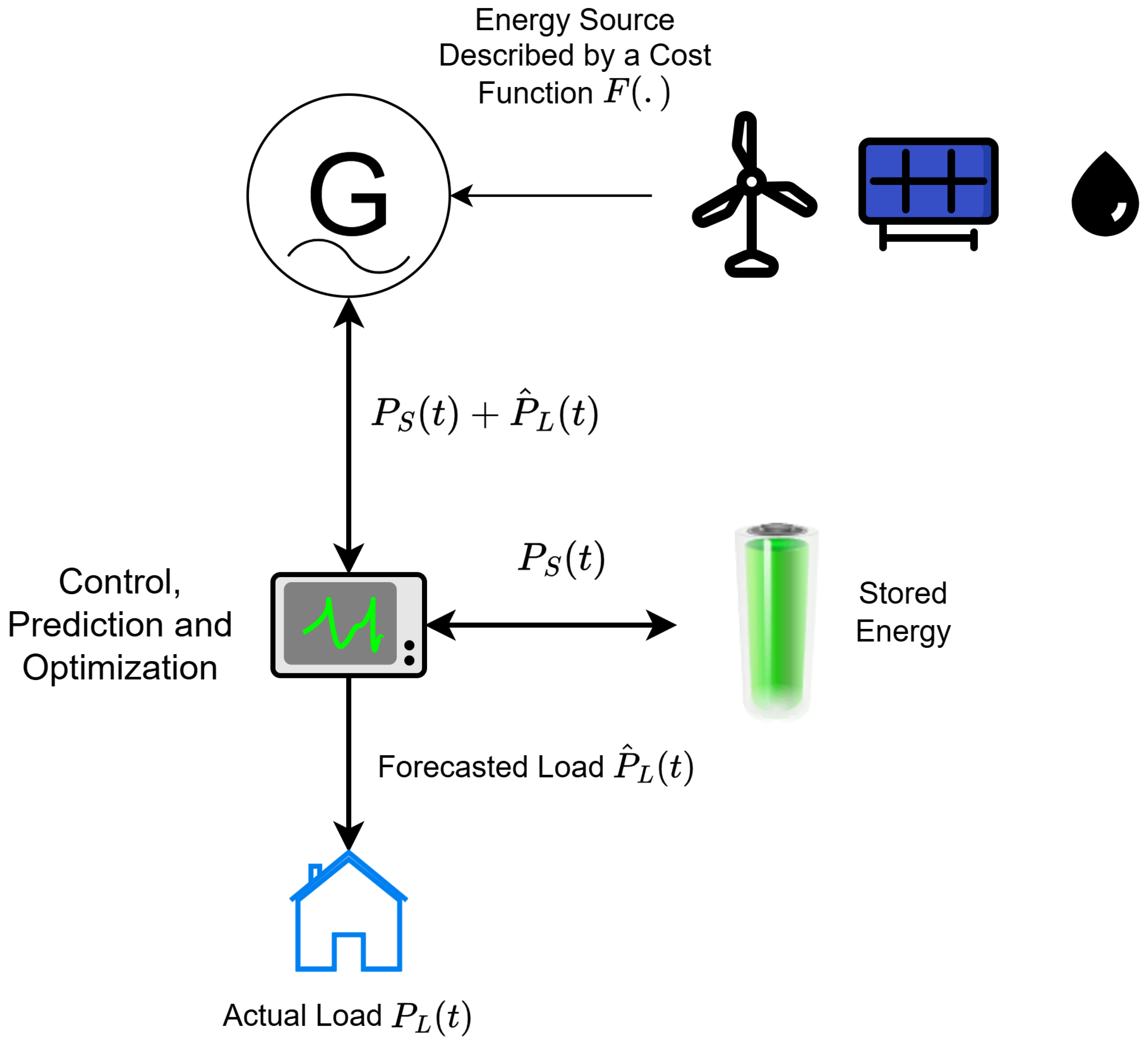
We consider a simplified power system composed of a controllable generation unit, an uncontrollable load, and an energy-storage device, as illustrated in Figure 3. The system operates as a single-bus microgrid, where the generated power can either supply the load directly or be routed into storage through a control and optimization unit. Although the framework naturally extends to multi-bus or network-level settings, we focus on the single-bus case for clarity.

In accordance with the classical energy-band formulation of the Shortest-Path method, the storage device is modeled as ideal and lossless. This assumption enables an analytical solution and isolates the effect of forecasting and control decisions from secondary efficiency losses. Incorporating realistic charging and discharging efficiencies can be addressed in future studies.

For consistency across daily cycles, we assume that the storage unit begins each day fully discharged and returns to the same state by the end of the day. Thus, all energy stored during the day is released within the same horizon, reflecting typical daily peak-shaving operation without long-term energy accumulation.

In this work, we intentionally do not include a monetary cost–benefit analysis or explicit modeling of battery degradation, cycling cost, round-trip efficiency, or C-rate limits. A full economic evaluation requires many system-specific assumptions—battery chemistry, aging coefficients, energy tariffs, reserve activation cost, and market participation rules—which differ widely across applications. Including a particular cost model would therefore reduce the generality and analytic clarity of the proposed framework.

Instead, the operational penalty defined in Section 4.3 serves as a system-agnostic proxy for operational cost. By weighting under- and over-generation differently, this metric captures the practical consequences of imperfect forecasts (e.g., unmet demand vs. curtailment) without committing to a specific economic model. This choice preserves generality while enabling meaningful comparison of forecasting and storage strategies within the FISP framework.

At each time step t, the system determines the generation level $p_g\left(t\right)$ and storage power $p_s\left(t\right)$ that satisfy the power balance while minimizing the peak of $p_g\left(t\right)$. The corresponding optimization formulation is presented in (7). The classical Shortest-Path algorithm computes the optimal generation trajectory when the full load profile is known a priori.

The proposed FISP framework removes this limitation by incorporating the forecasted load profile ${\widehat{P}}_L\left(t\right)$, produced by the ARMA and LSTM models, into the optimization layer, enabling systematic evaluation of forecast-driven operational deviations.

4.2. Process Flow and Optimization Layer

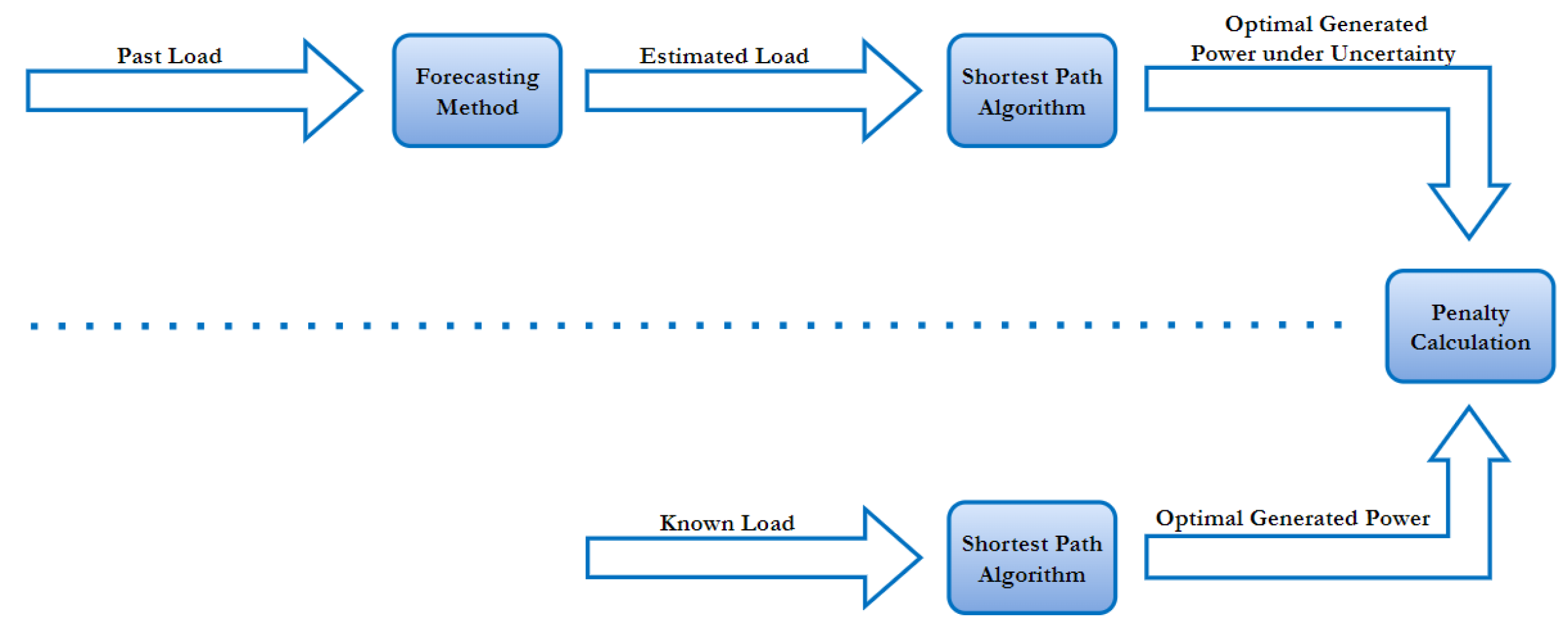
The proposed FISP framework integrates load forecasting and generation optimization through a sequential pipeline. Historical load data are first used to train the forecasting models, which produce predicted load profiles ${\widehat{P}}_L\left(t\right)$. These forecasts are then supplied to the shortest-path optimization algorithm $\varphi (·)$, which computes the corresponding optimal generation trajectory under forecast uncertainty. For benchmarking, the same optimization procedure is applied to the actual load profile $P_L\left(t\right)$, yielding the reference optimal generation trajectory.

The reference trajectory $\varphi \left(P_L\left(t\right)\right)$ represents the ideal solution achievable with complete knowledge of the true load. It serves as a benchmark for quantifying the degradation in operational performance arising solely from forecast uncertainty, independent of real-world control or actuation imperfections. Accordingly, the deviation between $\varphi \left(P_L\left(t\right)\right)$ and $\varphi ({\widehat{P}}_L\left(t\right))$ isolates the pure effect of forecast error on the optimization outcome.

The two trajectories are subsequently compared using the proposed penalty metric, which measures the operational impact of forecasting inaccuracies. The overall process of the FISP framework is illustrated in Figure 4, where load forecasts generated by ARMA and LSTM models are processed through the shortest-path optimization layer and evaluated using the penalty-based performance measure.

4.3. Penalty Metric Definition

To assess the effectiveness of the proposed method, we define a penalty metric that quantifies the deviation between the optimal generation profile obtained using the forecasted load and that derived from the actual load. The Shortest-Path algorithm, denoted by $\varphi (·)$, is applied to both the predicted load profile ${\widehat{P}}_L$ and the actual load profile $P_L$, generated by either the LSTM or ARMA forecasting models.

In this work, we distinguish between two types of generation errors that may occur when the optimization operates on forecasted load data rather than on the true load profile:

• Under-generation- when the produced power is insufficient to meet the true demand, leading to an unmet load. This is considered the more severe case.
• Over-generation- when the generated power exceeds the actual demand, while the surplus energy could, in principle, be stored or curtailed, it still represents a deviation from the optimal schedule.

To reflect the relative importance of these two cases, the total penalty is formulated as a weighted sum of the under- and over-generation components. A weighting factor $\alpha \in [0,1]$ determines the relative severity, with larger values of $\alpha$ penalizing under-generation more strongly. The computation process is summarized in Algorithm 1.

Algorithm 1 Computation of Weighted Penalty Metric

1: Initialize $R_{\mathrm{under}}=0$, $R_{\mathrm{over}}=0$

2: for $t=1$ to N do

3:        $\mathrm{\Delta }=\varphi \left(P_L\left(t\right)\right)-\varphi \left({\widehat{P}}_L\left(t\right)\right)$

4:        if $\mathrm{\Delta }>0$ then

5:            $R_{\mathrm{under}}\leftarrow R_{\mathrm{under}}+\left|\mathrm{\Delta }\right|$

6:        else

7:            $R_{\mathrm{over}}\leftarrow R_{\mathrm{over}}+\left|\mathrm{\Delta }\right|$

8:        end if

9: end for

10: $R_{\mathrm{total}}=\alpha ·R_{\mathrm{under}}+(1-\alpha )·R_{\mathrm{over}}$

The resulting penalty is normalized by the total optimal generation obtained under the actual load, ensuring independence from absolute power levels. The normalized penalty metric is therefore expressed as

$$R\left(\varphi \left({\widehat{P}}_L\right)\right)={\displaystyle \frac{R_{\mathrm{total}}}{{\sum }_{t=1}^N\varphi \left(P_L\left(t\right)\right)}}.$$

(9)

A smaller value of $R\left(\varphi \left({\widehat{P}}_L\right)\right)$ indicates higher alignment between the forecast-based and true optimal generation trajectories, demonstrating greater robustness of the forecasting model when integrated within the proposed FISP optimization framework. Empirically, we observe that while ARMA tends to exhibit larger over-generation components, LSTM achieves lower total penalties with smaller deviations of both types, indicating superior operational reliability.

5. Data and Forecasting Framework

5.1. Data and Preprocessing

The load datasets employed in this study were obtained from the ENTSO-E Transparency Platform—the official data repository of the European Network of Transmission System Operators for Electricity. ENTSO-E provides publicly accessible, high-resolution time-series records of electricity demand, generation, and system operation across all European member states [27].

Our analysis uses national load consumption data from Germany and Italy covering the years 2015—2023, with 2024 reserved exclusively for testing. Only weekday profiles were retained, as weekend demand exhibits fundamentally different behavioral patterns that can degrade forecasting performance if mixed with working-day dynamics.

To enhance model generalization and capture distinct seasonal characteristics, the datasets were separated by both country and season. Germany was selected for the summer period (June–September), representing an industrial system with a largely self-sufficient generation mix and relatively stable domestic demand.

Italy was selected for the winter period (December–February), where heating-driven consumption and higher import dependence create a a complementary operational scenario. This dual-region, dual-season configuration enables evaluation of the proposed FISP framework under diverse operational conditions.

Due to recent updates in ENTSO-E reporting formats, the German summer dataset is available at 15 min resolution, whereas the Italian winter dataset is available at 1 h resolution. Since each model is trained and evaluated solely within its own seasonal dataset, these differences in temporal granularity do not compromise cross-country comparability; results are examined in relative terms rather than direct numerical error values.

5.2. Model Architectures and Training Strategy

5.2.1. Data Splitting and Training Protocol

All forecasting models were trained using absolute power values (MW) to retain physical interpretability. Normalization was applied only during the evaluation stage to compare performance across countries and seasons with different demand magnitudes.

Because electricity consumption evolves gradually over time and exhibits strong temporal dependencies, the datasets were partitioned strictly chronologically. Random sampling across years would mix structurally different demand regimes and introduce information leakage, artificially improving validation accuracy. Instead, we adopted the following time-ordered structure:

• Training set (2015–2020) used for learning model parameters.
• Validation set (2021–2023) used exclusively for hyperparameter tuning and model selection.
• Test set (2024) a completely unseen year reserved for final performance evaluation.

Within each training block, individual days were randomly shuffled during mini-batch construction to stabilize gradient descent and reduce sensitivity to local temporal patterns. However, the global chronological order between the training, validation, and test sets was strictly preserved. This setup mirrors real-world deployment, where forecasting models must generalize from historical data to future demand without access to upcoming trends.

5.2.2. LSTM Architecture

The LSTM model is designed as a sequence-to-sequence predictor that maps one day’s load profile to the next day’s profile. Its architecture consists of a stack of LSTM layers followed by a nonlinear readout module. The fixed architectural components are summarized in

Table 1. LSTM Architecture and Training Configuration (shared across all experiments).

Component	Specification
Input dimension	1 feature (MW)
LSTM layers	D stacked layers (tuned)
Hidden units per layer	H units (tuned)
Fully connected layer	100 neurons
Activation	ReLU
Dropout layer	rate $\rho$ (tuned)
Output layer	1 regression output (MW)
Loss function	MSE
Optimizer	Adam
Mini-batch size	20
Training epochs	300

.

Hyperparameters were optimized using random search within MATLAB R2025a Experiment Manager. Random search offers strong empirical performance for low-dimensional hyperparameter spaces and provides a good compromise between efficiency and exploration. Separate hyperparameter searches were conducted for German summer data and Italian winter data, reflecting their structurally different load patterns.

The tuned hyperparameters are listed in

Table 2. Optimal LSTM hyperparameters for German summer and Italian winter datasets.

Hyperparameter	Germany (Summer)	Italy (Winter)
Number of LSTM layers D	3	3
Hidden units per layer H	59	60
Initial learning rate	0.000908	0.008909
Dropout rate $\rho$	0.262	0.548

. These values were selected based on the lowest mean absolute error on the season-specific validation set.

Once trained, the LSTM models were used to generate day-ahead forecasts for the year 2024, which were subsequently evaluated through the FISP optimization layer described in Section 4.2.

5.2.3. ARMA Model

To provide a transparent statistical baseline for comparison, we trained seasonal ARMA models using a systematic grid-search procedure. In the ARMA framework, the autoregressive and moving-average orders $(p,q)$ fully determine the model structure; therefore, these values serve as the model’s hyperparameters.

We evaluated all combinations in the ranges resulting in 80 distinct ARMA configurations. For each candidate pair $(p,q)$:

• The model was fitted to the training years using maximum-likelihood estimation.
• Day-ahead forecasts were generated sequentially for the validation years.
• The Mean Absolute Error (MAE) was computed over all validation days.
• Non-convergent or non-stationary models were automatically skipped.

This search identifies the ARMA order that best captures the temporal dynamics of each seasonal dataset without imposing assumptions about correlation length or linearity scale.

Crucially, the grid search yielded different optimal ARMA orders for summer and winter, reflecting the distinct load variability and peak timing patterns characteristic of each season. This result confirms that the ARMA model is sensitive to seasonal statistical structure and must therefore be trained separately for each dataset.

The resulting optimal orders are summarized in

Table 3. Optimal ARMA hyperparameters selected via grid search. Seasonal differences in temporal structure lead to different optimal orders, highlighting the necessity of season-specific ARMA training.

Season	Optimal p	Optimal q
Germany Summer	5	5
Italy Winter	7	3

.

Unlike the LSTM, which automatically learns nonlinear dependencies through its hidden state and depth, the ARMA model must explicitly encode temporal correlations via its $(p,q)$ parameters.

The observed differences in seasonal optimal orders reflect this limited flexibility: ARMA adapts to the exact statistical structure of each season, whereas the LSTM inherently generalizes across more complex patterns.

This motivates the use of the LSTM forecasts as the principal predictive component in the FISP framework, while retaining ARMA as a transparent and interpretable baseline.

6. Operational Evaluation via FISP

6.1. Forecasting Performance

To evaluate the quality of the short-term load forecasts, we compare two representative prediction models: a Long Short–Term Memory (LSTM) neural network and an Autoregressive Moving Average (ARMA) model. Both models were trained and evaluated on the same chronologically partitioned datasets described in Section 5. Forecast accuracy was quantified over the entire test year using the Mean Absolute Error (MAE).

Across the full evaluation period, the LSTM model achieved substantially lower MAE compared with the ARMA baseline, indicating a closer match to the true load dynamics. This behavior is expected: the LSTM architecture can capture nonlinear temporal dependencies and state transitions, whereas ARMA is limited to fixed linear relationships and cannot adapt to rapidly changing load shapes.

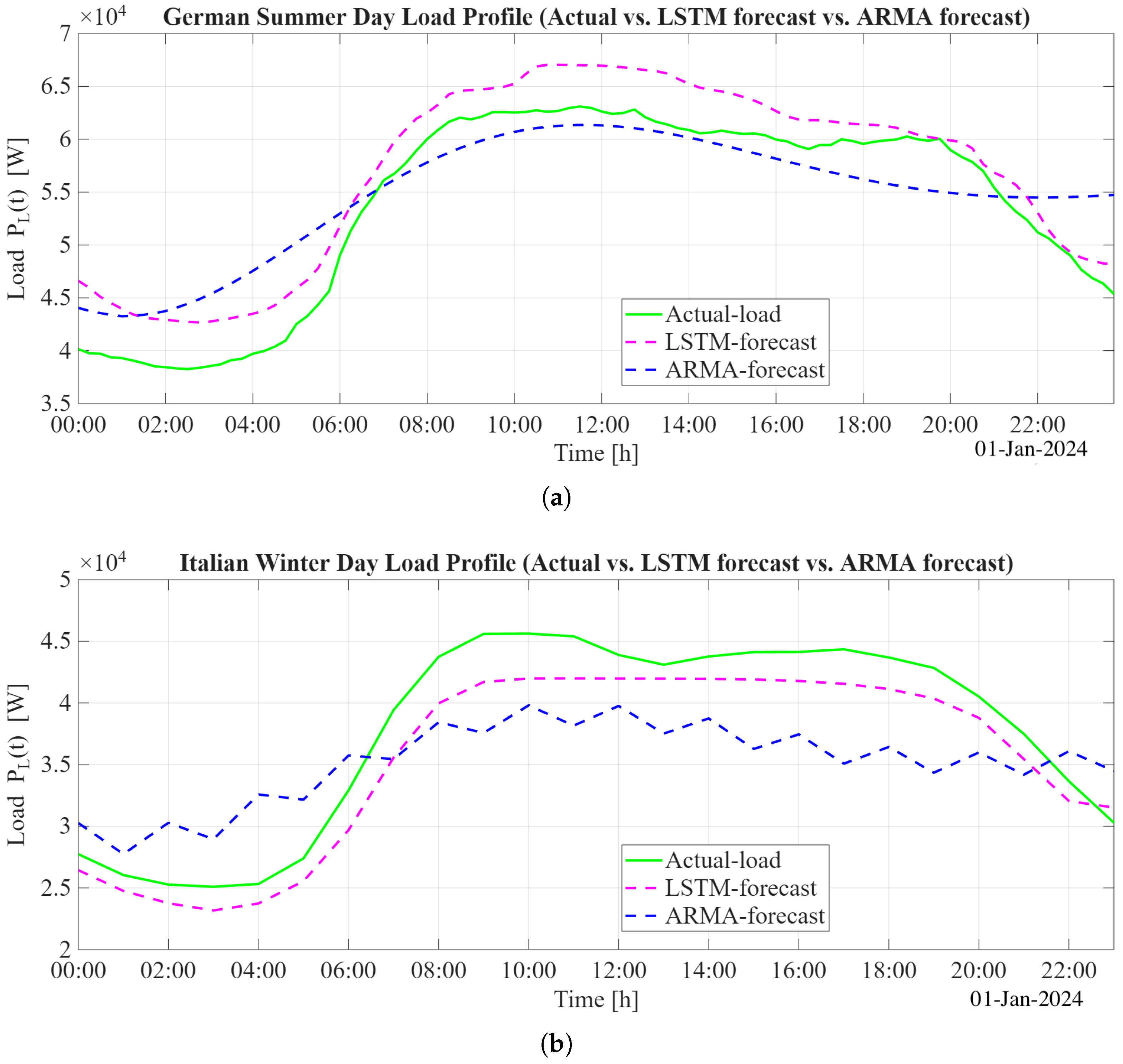
To provide a qualitative illustration, Figure 5 shows both forecasts alongside the actual load for a representative test day. The LSTM forecast tracks the true demand profile more closely throughout the morning ramp-up and evening decline. In contrast, the ARMA model reproduces the overall diurnal trend but exhibits noticeable lag during sharp transitions and tends to underestimate the evening load.

Importantly, these day-level examples are consistent with the aggregate statistical evaluation: the LSTM model provides more accurate and responsive forecasts than the ARMA model across the full test horizon. These forecasts serve as the input to the shortest-path smoothing procedure presented in Section 3.2, enabling an integrated assessment of prediction quality and storage-aware penalty minimization.

Graphical Illustration of the Penalty Metric

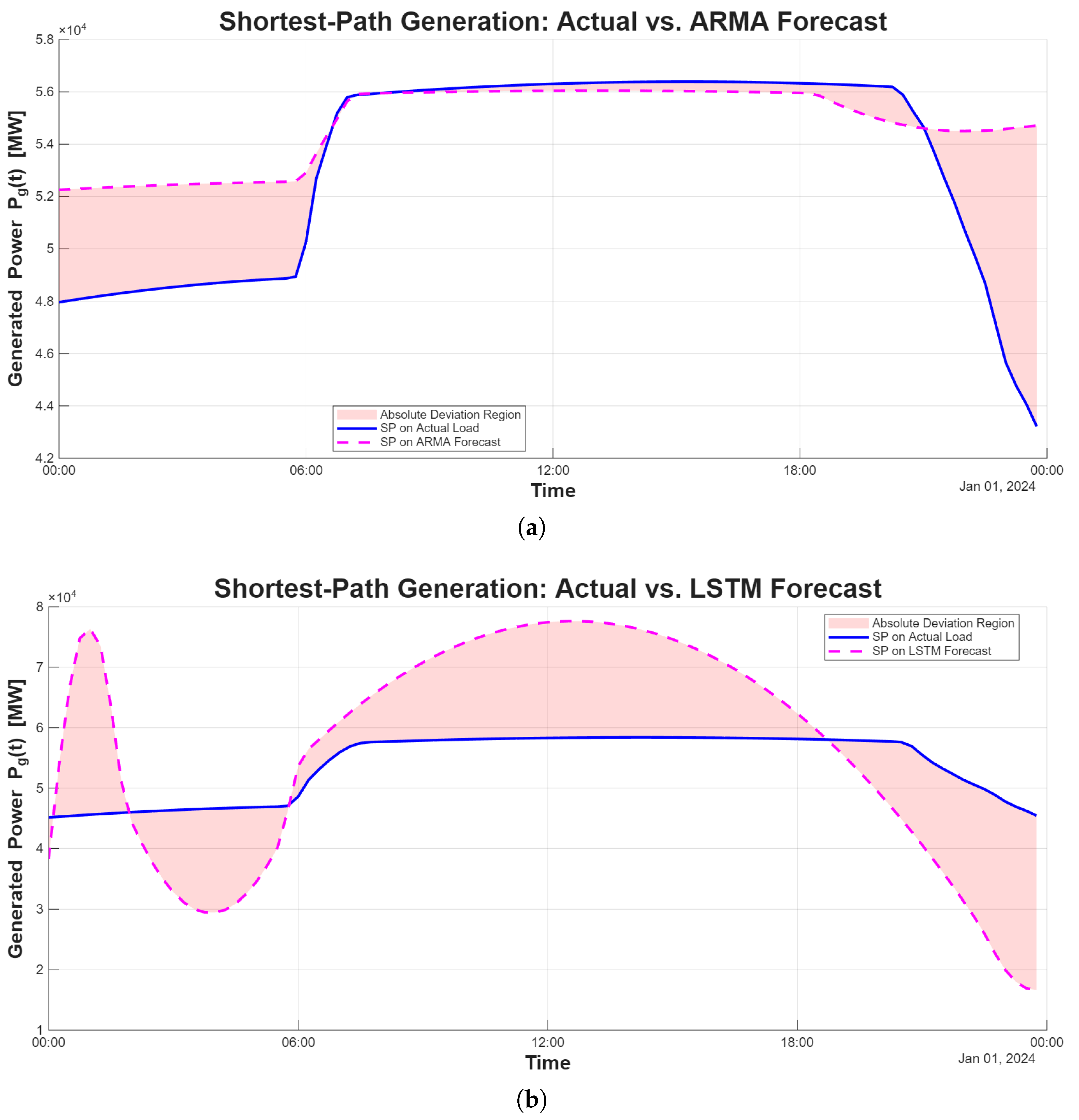
After generating the LSTM- and ARMA-based forecasts, each predicted load profile was processed through the shortest-path operator $\varphi (·)$ described in Section 4. This step maps a load trajectory into the corresponding optimal generation trajectory under the assumed storage capacity. To visualize the penalty construction in (9), Figure 6 compares, for a representative German summer test day and a fixed storage capacity, the optimal generation trajectory obtained from the true load profile with those derived from the LSTM and ARMA forecasts. In each panel, the solid curve denotes the optimal generation $p_g\left(t\right)$ computed from the actual load, while the dashed curve shows the generation trajectory resulting from the forecasted load. The shaded region represents the absolute deviation $|\varphi \left(P_L\left(t\right)\right)-\varphi ({\widehat{P}}_L\left(t\right))|$ at each time step, which corresponds to the numerator of the weighted penalty metric.

Panel (a) shows the case of the ARMA forecast. The deviation region is concentrated mostly above the actual-operation curve, indicating that the ARMA-based trajectory tends to over-generate relative to the ideal schedule. In contrast, panel (b) presents the LSTM-based forecast, where the deviation region is more balanced and includes intervals of both over- and under-generation.

Because the weighted penalty assigns a higher cost to under-generation (via the factor $\alpha >0.5$), this asymmetry helps explain why the ARMA-based penalties can be numerically smaller in some settings: the ARMA forecast is not more accurate in a symmetric sense, but it tends to err on the conservative side by producing more energy than required. This single-day visualization therefore clarifies the qualitative difference between the two forecasting models and illustrates how the choice of weighting in the penalty metric shapes the resulting assessment of operational risk.

6.2. Determination of Storage Capacity Range

To explore the influence of storage capacity on peak-shaving performance, we first establish a data-driven upper bound on the feasible storage size. To do so, we compute the theoretical amount of energy that an unconstrained, lossless storage device would exchange under the ideal shortest–path solution.

For each test-day d, we compute the optimal storage trajectory using the Shortest-Path algorithm under the assumption of effectively infinite storage capacity. This yields the maximum amount of energy that would be stored on that day if the device were unconstrained. For a given day d, let

$$W_s^{\left(d\right)}\left(t\right)=W_g^{\left(d\right)}\left(t\right)-W_L^{\left(d\right)}\left(t\right)$$

(10)

denote the optimal stored-energy trajectory. The maximal storage utilization for that day is

$$E_{max}^{\left(d\right)}=\underset{t}{max}{W}_s^{\left(d\right)}\left(t\right).$$

(11)

This value represents the minimum storage size required for that day to achieve perfect (unconstrained) shortest–path smoothing. To obtain a capacity that guarantees perfect smoothing for all days in the test set, we take the maximum over all daily requirements,

$$E_{max}=\underset{d}{max}{E}_{max}^{\left(d\right)}.$$

(12)

Thus, $E_{max}$ is the smallest storage capacity that enables the ideal shortest–path trajectory on every test day, while any smaller device would be insufficient for at least one day. It therefore defines a natural normalization scale for evaluating the impact of finite storage. All experiments in Section 6 use storage capacities expressed as fixed percentages of $E_{max}$.

6.3. Quantitative Penalty Evaluation Across Storage Capacities

We now analyze how storage capacity influences the operational penalty defined in Section 4.3. For each storage level, the shortest-path (SP) operator is applied to the actual load and to the load forecasted by either the LSTM or ARMA model. The resulting penalty quantifies the deviation between the forecast-driven schedule and the ideal schedule derived from perfect load information

A key observation from

Table 4. Average penalty values for different storage capacities using LSTM and ARMA forecasts (Germany–summer dataset).

Storage Size (Relative to (12))	LSTM $\overline{\mathit{R}}\left(\mathit{\varphi }\left({\widehat{\mathit{P}}}_{\mathit{L}}\right)\right)$	ARMA $\overline{\mathit{R}}\left(\mathit{\varphi }\left({\widehat{\mathit{P}}}_{\mathit{L}}\right)\right)$
5%	$0.0308$	$0.019$
10%	$0.0501$	$0.0187$
20%	$0.0637$	$0.0183$
30%	$0.0867$	$0.0179$
40%	$0.1275$	$0.0177$
100%	$0.2427$	$0.0141$

and

Table 5. Average penalty values for different storage capacities using LSTM and ARMA forecasts (Italy winter dataset).

Storage Size (Relative to (Relative to (12))	LSTM $\overline{\mathit{R}}\left(\mathit{\varphi }\left({\widehat{\mathit{P}}}_{\mathit{L}}\right)\right)$	ARMA $\overline{\mathit{R}}\left(\mathit{\varphi }\left({\widehat{\mathit{P}}}_{\mathit{L}}\right)\right)$
5%	$0.0445$	$0.0621$
10%	$0.0402$	$0.0625$
20%	$0.0803$	$0.0617$
30%	$0.1887$	$0.0621$
40%	$0.1271$	$0.0535$
100%	$0.1659$	$0.0316$

is that, under the weighted penalty definition, the deviation between the forecast-based and the true-load-based SP trajectories increases with the storage capacity. This trend is natural and reflects an important property of the SP operator: As storage becomes larger, the SP operator possesses greater flexibility and therefore reacts more aggressively to the predicted load profile. When the forecast is not perfect, these amplified charge–discharge actions generate correspondingly larger deviations from the true optimal trajectory, leading to an increase in the penalty. In this sense, larger storage magnifies the operational impact of forecasting error.

The LSTM-induced deviations grow with capacity, but they remain tightly bounded, reflecting stable forecast-to-operation consistency. This indicates that the LSTM forecasts—although not perfect—are sufficiently accurate for the SP operator to make beneficial use of the available flexibility.

In contrast, the ARMA forecasts are substantially noisier and less aligned with the true load dynamics. As a result, enlarging the storage reservoir does not systematically reduce their penalty; the SP operator cannot leverage additional flexibility when the underlying forecast is too inaccurate to guide meaningful charge–discharge decisions.

Notably, ARMA may occasionally yield lower penalties at small storage levels due to its tendency to over-generate, which is less heavily weighted under the asymmetric penalty metric. However, this behavior does not translate into more reliable or consistent performance as storage increases.

In summary, the quantitative results demonstrate that while larger storage amplifies the effect of forecasting errors for both models, the LSTM forecasts maintain significantly stronger alignment with the true-load-based SP trajectory. The ARMA driven system does not benefit from increased flexibility, as forecast inaccuracy prevents meaningful optimization. These findings reinforce the suitability of LSTM forecasting as the predictive front-end of the proposed FISP framework.

6.4. Qualitative Comparison of FISP Operation Under Actual and Forecasted Loads

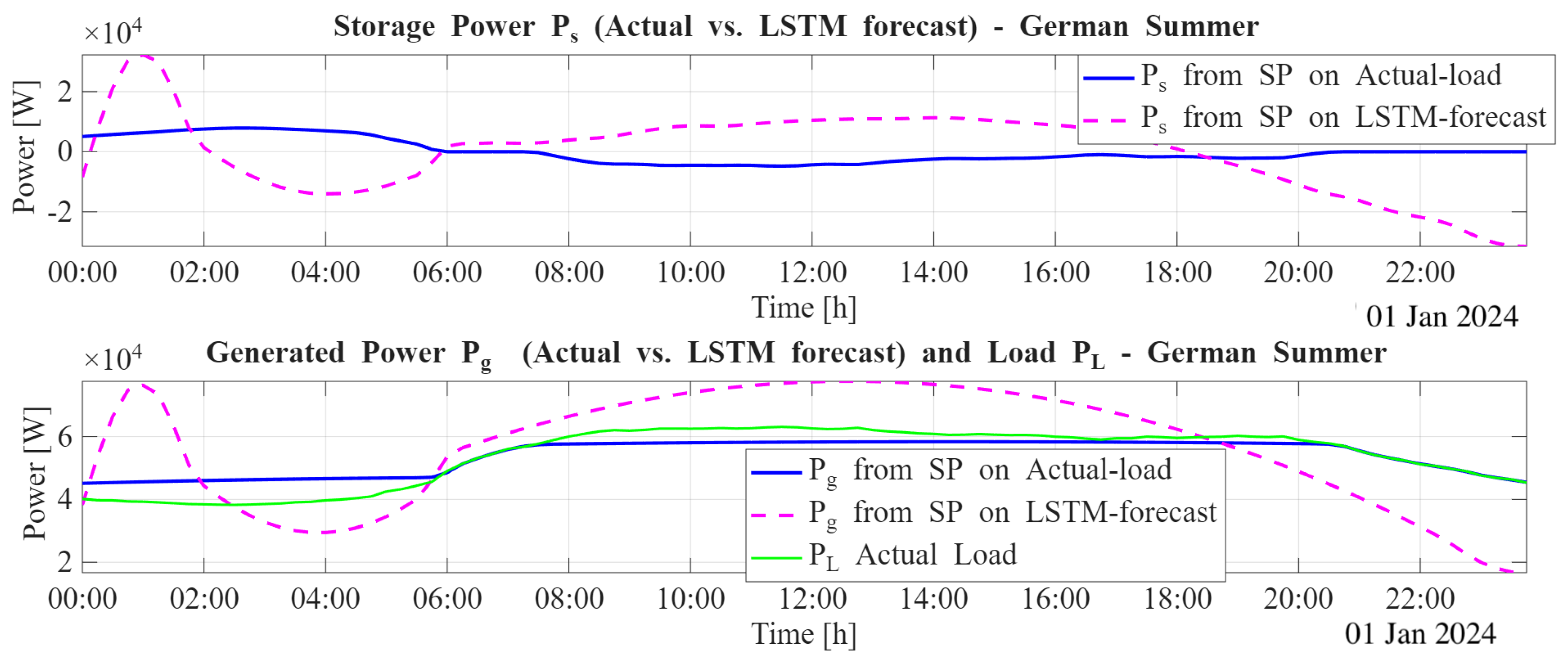
To complement the quantitative penalty results, we provide a qualitative comparison of the FISP–optimized operation obtained using the actual load profile and the LSTM-forecasted load profile. Figure 7 presents, for a representative summer test day, the storage power $p_s\left(t\right)$ and generation power $p_g\left(t\right)$ trajectories resulting from the shortest-path optimization.

The upper panel illustrates how the storage unit reacts when the controller operates with perfect knowledge (actual load) versus imperfect information (LSTM forecast). Even relatively small forecast deviations generate visible differences in charge–discharge behavior. This is expected: the shortest-path operator is highly sensitive to the slope of the input load, since it determines both the direction and timing of storage actions.

The lower panel shows the corresponding generation trajectories $p_g\left(t\right)$ alongside the load profiles. Here, the effect of forecast errors becomes more pronounced. Because the shortest-path algorithm attempts to remain on one of the optimal energy boundaries, even small load mismatches can lead to amplified differences in the generated power. This amplification is a known and intrinsic property of boundary-based optimal scheduling and does not indicate instability or over-reaction; rather, it reflects the algorithm’s attempt to maintain feasibility under a perturbed input signal.

Despite these local differences, the overall temporal structure of the two trajectories remains aligned: both solutions exhibit the same broad phases of supply, storage use, and return to baseline. This confirms that the LSTM-driven FISP operation preserves the main qualitative attributes of the ideal schedule derived from perfect load knowledge.

These observations are consistent with the penalty trends in Table 4 and Table 5: for both datasets, LSTM-based operation remains close to the ideal trajectory, whereas ARMA-based operation exhibits larger deviations. The qualitative plot thus reinforces the core conclusion of this study: integrating deep-learning forecasts within the shortest-path framework yields an operational behavior that stays robust, structured, and physically consistent even in the presence of forecast uncertainty.

7. Discussion

The results reveal a nuanced interaction between forecasting accuracy, storage capacity, and the structure of the shortest-path (SP) optimization. Several key insights emerge from the analysis.

7.1. Forecast Quality and Operational Behavior

Across both datasets, the LSTM forecasts consistently outperform ARMA in terms of numerical accuracy. However, the operational impact of these errors depends strongly on the storage size. The SP operator is highly sensitive to variations in the input load: even small discrepancies in the forecasted profile can lead to amplified differences in the resulting power and storage trajectories. This behavior is intrinsic to boundary-based optimal scheduling and should not be interpreted as instability. Instead, it highlights that the SP solution reflects structural differences in the signals rather than direct pointwise error.

7.2. Role of Storage Capacity

The penalty results demonstrate that storage capacity plays a decisive role in absorbing forecast mismatches. For moderate to large reservoirs, the SP solution becomes more responsive to deviations between the actual and forecasted loads. This increased reactivity can lead to higher penalties for larger capacities when the forecast errors are sufficiently structured, as observed in both datasets. Importantly, this trend does not imply degraded performance; rather, it reflects a shift in operational regime where the available flexibility allows the SP to follow different optimal boundaries under each input profile.

In contrast, when storage is very small, the SP solution is constrained and therefore less sensitive to forecast errors—resulting in artificially lower penalties. This helps explain why the penalty does not always decrease with storage size under the new metric.

7.3. Comparison Between LSTM and ARMA

Despite these effects, LSTM-based operation generally remains closer to the ideal schedule derived from the true load, especially in terms of qualitative trajectory structure. ARMA-based results exhibit larger deviations and, in many cases, reduced sensitivity to storage flexibility, consistent with the limited expressiveness of linear time-series models. The penalty trends for ARMA are comparatively flat, reflecting that the forecast quality is not sufficient for additional storage to provide operational benefit.

7.4. Implications for Practical Deployment

These observations suggest that forecasting accuracy and physical flexibility interact in non-trivial ways. High-quality forecasts enable storage to be used effectively, while poorer forecasts may render additional capacity less useful or even counterproductive under aggressive scheduling. For grid operators, this highlights the importance of jointly considering forecasting strategy and storage dimensioning rather than optimizing them independently.

Overall, the study demonstrates that the FISP framework provides a robust and operationally interpretable link between prediction and optimal scheduling. Even under uncertainty, the integration of forecasting and shortest–path optimization yields structured, physically consistent operation and offers a principled pathway for coordinating storage and generation at scale.

8. Conclusions

This work introduced the Forecast-Integrated Shortest Path (FISP) framework, a principled method for combining load forecasting with boundary-based optimal scheduling. By integrating forecasting models such as LSTM and ARMA into the shortest–path operator, the framework enables peak-shaving decisions under realistic, forward-looking conditions rather than assuming perfect knowledge of the load. A weighted penalty metric was developed to quantify the operational impact of forecast uncertainty. The results showed that forecasting accuracy and storage flexibility interact in nontrivial ways: larger reservoirs allow the SP operator to react more aggressively to structure in the forecasted load, which can magnify differences between the forecast-based and ideal trajectories. Across both datasets, LSTM forecasts generally maintained closer qualitative alignment with the true load, whereas ARMA demonstrated limited sensitivity to storage capacity.

The findings highlight that forecasting quality and storage sizing must be considered jointly when designing real-world peak-shaving strategies. Future work should expand the analysis to additional seasons, incorporate weather and event features, explore advanced models such as Transformers, and include practical considerations such as storage losses, inverter constraints, and generator cost functions.

Overall, the FISP framework provides a scalable and interpretable bridge between prediction and optimal operation, demonstrating how forecasting and storage management can be co-designed to support reliable and efficient grid operation.