Article

Demand Response Potential Evaluation Based on Multivariate Heterogeneous Features and Stacking Mechanism

by
Chong Gao
1,
Zhiheng Xu
1,
Ran Cheng
1,
Junxiao Zhang
1,
Xinghang Weng
1,
Huahui Zhang
2,
Tao Yu
2 and
Wencong Xiao
2,*
1
Power System Planning Research Center of Guangdong Power Grid Co., Ltd., Guangzhou 510623, China
2
School of Electric Power Engineering, South China University of Technology, Guangzhou 510641, China
*
Author to whom correspondence should be addressed.
Energies 2026, 19(1), 194; https://doi.org/10.3390/en19010194 (registering DOI)
Submission received: 31 October 2025 / Revised: 21 December 2025 / Accepted: 25 December 2025 / Published: 30 December 2025
(This article belongs to the Section F1: Electrical Power System)

Abstract

Accurate evaluation of demand response (DR) potential at the individual user level is critical for the effective implementation and optimization of demand response programs. However, existing data-driven methods often suffer from insufficient feature representation, limited characterization of load profile dynamics, and ineffective fusion of heterogeneous features, leading to suboptimal evaluation performance. To address these challenges, this paper proposes a novel demand response potential evaluation method based on multivariate heterogeneous features and a Stacking-based ensemble mechanism. First, multidimensional indicator features are extracted from historical electricity consumption data and external factors (e.g., weather, time-of-use pricing), capturing load shape, variability, and correlation characteristics. Second, to enrich the information space and preserve temporal dynamics, typical daily load profiles are transformed into two-dimensional image features using the Gramian Angular Difference Field (GADF), the Markov Transition Field (MTF), and an Improved Recurrence Plot (IRP), which are then fused into a single RGB image. Third, a differentiated modeling strategy is adopted: scalar indicator features are processed by classical machine learning models (Support Vector Machine, Random Forest, XGBoost), while image features are fed into a deep convolutional neural network (SE-ResNet-20). Finally, a Stacking ensemble learning framework is employed to intelligently integrate the outputs of base learners, with a Decision Tree as the meta-learner, thereby enhancing overall evaluation accuracy and robustness. Experimental results on a real-world dataset demonstrate that the proposed method achieves superior performance compared to individual models and conventional fusion approaches, effectively leveraging both structured indicators and unstructured image representations for high-precision demand response potential evaluation.

1. Introduction

With the increasing global energy demand and the growing integration of renewable energy sources, modern power systems are confronted with unprecedented challenges and opportunities [1]. To address these challenges and enhance grid flexibility and operational efficiency, demand response has emerged as a pivotal enabling strategy and has been extensively studied and deployed. Demand response plays a critical role in balancing electricity supply and demand, alleviating grid congestion, and improving the reliability and sustainability of power systems [2]. Moreover, by enabling demand-side adaptability, it facilitates the effective utilization of intermittent renewable generation [3]. However, accurate demand response potential evaluation at the individual user level remains a fundamental prerequisite for the successful implementation and optimization of demand response programs [4].
In existing research, the extraction of demand response (DR) resource characteristics and the evaluation of DR potential have been explored from multiple perspectives. Wang proposed a large-scale resource potential inference framework based on fuzzy set theory and principal component analysis (PCA). The core idea is to handle uncertainties in user behavior and external factors through fuzzy sets and to identify key influencing parameters via dimensionality reduction with PCA. This method offers good interpretability at the system level but has limited capability in characterizing fine-grained behaviors of individual users and relies on expert knowledge for defining fuzzy rules [5]. Luo constructed a residential user profiling model based on load adjustability and transferability characteristics, evaluating DR potential by extracting typical electricity consumption patterns. This study highlights the value of user behavior profiling in residential response assessment; however, the model does not sufficiently integrate dynamic external factors such as weather and electricity prices, limiting its generalizability across different scenarios [6]. Li employed price elasticity theory combined with support vector machine (SVM) regression to estimate users’ price responsiveness from historical data and thereby assess their incremental response potential. This approach has certain advantages in capturing nonlinear relationships between price signals and load changes, but it exhibits weak capability in fusing high-dimensional heterogeneous features and does not fully account for the temporal dynamics of load profiles [7]. Furthermore, Wang introduced set pair analysis (SPA) theory, which addresses uncertainty and ambiguity in DR evaluation by systematically analyzing identity, discrepancy, and contrary relationships within datasets. This method provides a novel perspective for uncertainty modeling in DR potential assessment; however, its outcomes depend heavily on the construction of indicator systems, and computational efficiency is relatively low at large-scale user levels. These studies each emphasize different methodological aspects but commonly suffer from insufficient feature representation, inadequate characterization of load profile dynamics, and a lack of differentiated fusion mechanisms for structured indicators and unstructured temporal information [8]. As a result, further improvements in evaluation accuracy and model generalization remain constrained.
Mechanism-driven models incorporate domain-specific knowledge and physical or behavioral constraints into their structures to study user electricity consumption behavior underprice-based control mechanisms, offering strong interpretability. However, these models typically rely on simplified linear or affine mappings between price signals and load adjustments, which limits their ability to accurately capture the inherent complexity, heterogeneity, and non-linear dynamics of actual user behavior [9,10,11].
Data-driven methods leverage large-scale historical data to automatically learn complex patterns. Rooted in real-world operational scenarios, this methodology analyzes massive volumes of metering and load data to extract valuable insights into users’ price-responsive behaviors, enabling more accurate modeling of the non-linear and time-varying characteristics of electricity consumption and thus providing a more realistic representation of actual usage patterns. Liang et al. [12] proposed a data-driven method to evaluate comprehensive energy and power response potential using smart meter data, enabling fine-grained analysis at the consumer level. However, such methods are typically highly dependent on data quantity and quality and, due to their “black-box” nature, often suffer from low transparency and poor interpretability, posing significant challenges for model validation, regulatory acceptance, and practical deployment [13,14].
Although data-driven methods have demonstrated significant potential in demand response potential evaluation, existing studies still exhibit notable limitations in feature utilization, data representation, and heterogeneous information fusion. First, most models rely on shallow or manually designed feature engineering, which hinders their ability to fully capture the complex interactions between user load patterns and external environmental factors (e.g., weather conditions, electricity prices). This results in insufficient representation of critical response-related information, thereby impairing model learning efficiency and discriminative capability [15]. Second, conventional methods typically represent load data in the form of numerical sequences or statistical features, lacking effective characterization of the overall shape and dynamic variation patterns of load profiles, which limits the model’s capacity to uncover deeper behavioral characteristics [16]. Third, when handling heterogeneous features—such as scalar metrics and electricity consumption curves—existing fusion strategies often adopt uniform or simplistic concatenation methods, lacking differentiated modeling mechanisms for distinct feature types. This may lead to information redundancy or suppression of salient features, ultimately degrading the model’s overall performance and generalization ability [17].
Therefore, this paper proposes a demand response potential evaluation method based on multivariate heterogeneous features and a Stacking-based fusion mechanism. The main contributions are summarized as follows:
(1)
To enhance model evaluation performance, multidimensional feature indicators are extracted from users’ historical electricity consumption data and associated external environments, ensuring effective representation of critical information relevant to demand response potential and providing the model with clear learning patterns.
(2)
To further expand the model’s information space, typical daily electricity consumption curves are transformed into image-based features and jointly utilized with indicator features in the evaluation process. The incorporation of image features enriches the input data modality and enables the model to more deeply uncover latent behavioral characteristics.
(3)
To address the fusion challenge of heterogeneous features, a differentiated input strategy is proposed. For scalar indicators, multiple classical machine learning models are employed; for image-based features, an SE-ResNet-20 model integrating a Squeeze-and-Excitation (SE) module is introduced. Finally, a Stacking ensemble mechanism is adopted to effectively integrate the outputs of sub-models, thereby further improving evaluation performance.
The following sections are organized as follows: Section 2 presents the overall framework of the proposed method. Section 3 details the feature extraction method for demand response potential evaluation. Section 4 describes the construction of the demand response potential evaluation model. Section 5 outlines the experimental setup and presents the results with comprehensive analysis. Finally, Section 6 concludes the study and discusses potential directions for future research.

2. Framework for Demand Response Potential Evaluation

The framework for demand response potential evaluation proposed in this paper is illustrated in Figure 1, consisting of the following steps:
(1)
Preprocess raw data to obtain typical daily electricity consumption curves for individual users.
(2)
Extract multivariate feature indicator features that characterize the demand response potential. Furthermore, the typical daily electricity consumption curve is transformed into image features, which, together with the multivariate indicator features, are used in the evaluation of demand response potential.
(3)
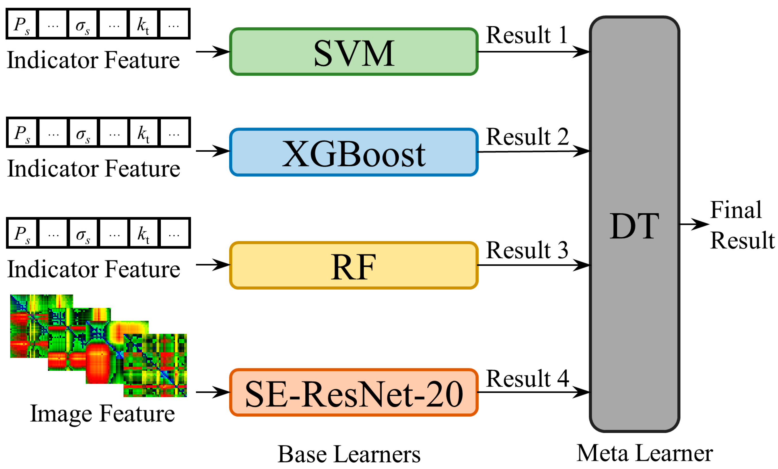
Construct the demand response potential evaluation model using Support Vector Machine (SVM), Random Forest (RF), XGBoost, and SE-ResNet-20 as base learners, and Decision Tree (DT) as the meta learner. Specifically, image features are input into SE-ResNet-20, while indicator features are input into the other base learners.
(4)
Train the demand response potential evaluation model based on both multivariate feature indicators and graphical features, followed by an analysis of the results.
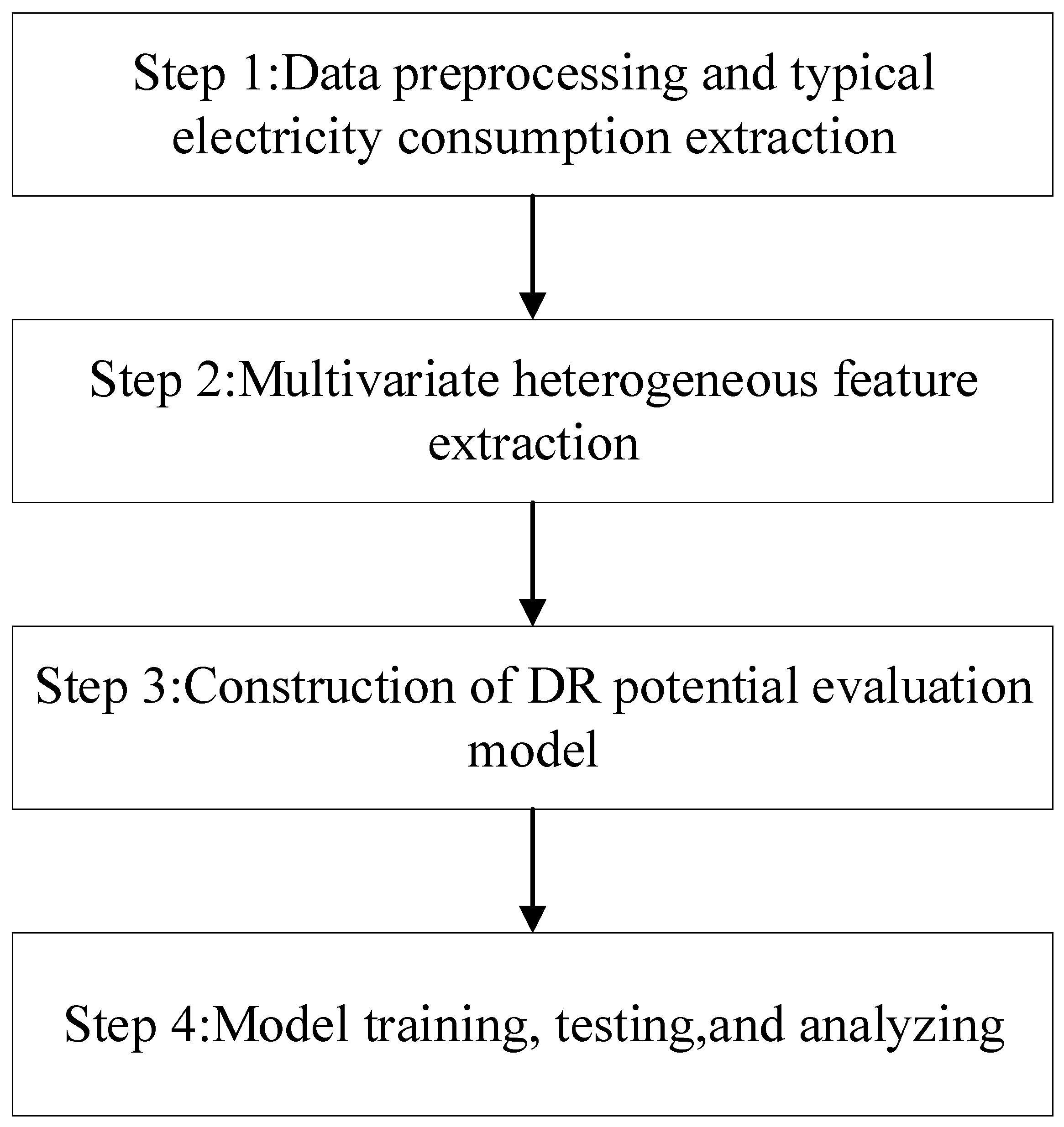
Figure 1. Flowchart of the proposed demand response potential evaluation method.
Energies 19 00194 g001

3. Heterogeneous Demand Response Potential Feature Extraction

3.1. Data Preprocessing

Due to issues such as equipment malfunctions or unstable communications, raw data inevitably suffers from data loss or anomalies. Preprocessing of such data is conducive to achieving more optimal and reliable evaluation results. For normally generated small-scale random data corruption (within a span of 6 h), which still holds analytical value, data can be repaired through outlier detection and by filling in with similar day load profiles.
Initially, historical electricity consumption data of individual users that have not participated in demand response are obtained from measurement devices. Specifically, given the differing data characteristics across various day types, data from working days and holidays are processed independently. This data is then transformed into a matrix format as shown below:
X = x 1 , 1 x 1 , 2 x 1 , j x 1 , N x 2 , 1 x 2 , 2 x 2 , j x 2 , N     x i , 1 x i , 2 x i , j x i , N     x M , 1 x M , 2 x M , j x M , N
where xi,j represents the electricity consumption of the user at the j-th sampling time on day i, M indicates the total number of days recorded, and N denotes the number of sampling points in one day. Each row Xi,: of the matrix represents the daily load profile for a specific date, while each column X:,j represents the historical electricity consumption at a specific sampling time.
Considering that the distribution of electricity consumption data is unknown and highly variable, this paper uses the Median Absolute Deviation (MAD) to detect outliers, which does not require assumptions about data distribution and exhibits high robustness against fluctuations. Additionally, considering that users’ electricity consumption patterns may have slight temporal variations, for the electricity consumption value at a specific time, historical data from one hour before and after that sampling point are selected. The absolute deviation between each data point and the median value Ei,j = xi,j − median (X:,j–⌈N/24⌉:j+⌈N/24⌉) is calculated, along with the median of these absolute deviations EMAD (i.e., MAD). For a data point under examination, a parameter n is set; if Ei,j > n × EMAD, the data point is identified as an outlier and excluded from further analysis, after which it is replaced by the imputed value derived from similar days. In this study, n is set to 3.5, which effectively filters out conspicuous outliers caused by metering faults or communication disturbances while preserving normal electricity consumption fluctuations.
The mean value from similar days is used to fill in missing values and the excluded outliers. Specifically, for the electricity consumption curve to be completed, the Euclidean distance between the non-missing portion and the corresponding parts of other daily electricity consumption curves is computed, as Euclidean distance effectively captures the overall similarity of daily load profiles. The 10 curves with the smallest Euclidean distances are selected. Using multiple nearest curves improves robustness and implicitly reflects similar operating conditions embedded in the load patterns. The average of the data at the corresponding missing time points from these curves is then used to fill the gaps.

3.2. Acquisition of Typical Daily Electricity Consumption Curves

Due to the large volume of historical load data and the fact that most data exhibit similar consumption patterns and characteristics, this section extracts typical daily electricity consumption curves from the historical data to reflect general user consumption behavior and features related to demand response potential, facilitating the subsequent methodology. The steps for extracting typical daily electricity consumption curves are as follows:
(1) Calculate the distance between daily electricity consumption curves in the historical data:
d i j = k = 1 M x i , k x j , k 2
where dij denotes the Euclidean distance between daily electricity consumption curve i and curve j.
(2) For each curve, compute the sum of its distances to all other curves:
Δ i = j i d i j
(3) Select the curve corresponding to the minimum as the medoid [18,19]. For each curve, compute the softmax weight wi based on its distance to the medoid curve m:
w i = exp d i m j = 1 M exp d j m
(4) Compute the typical daily electricity consumption curve l by taking a weighted average of all curves:
l = i = 1 M w i X i , :
Compared to directly averaging daily electricity consumption curves, this method ensures the central curve is an actual observed curve. By incorporating weighting, it balances central and group characteristics, effectively suppressing noise interference while avoiding excessive smoothing, resulting in a more stable and reliable representation.
Furthermore, to eliminate the influence of load magnitude and emphasize the relative shape of the load profile, each daily electricity consumption curve is normalized by dividing by its maximum value, as shown in Equation (6). The normalized typical daily electricity consumption curve l is then obtained by following the above steps.
x i , j * = x i , j max X i , :
Figure 2 presents the typical daily electricity consumption curves derived from three months of historical data for two representative users. The light-colored lines represent historical electricity consumption curves, while the dark-colored lines indicate the corresponding typical electricity consumption curves. The extracted typical curves reveal two distinct patterns of electricity-use behavior. For User 1, the electricity consumption exhibits a double-peak pattern, defined by pronounced morning and evening peaks separated by low-consumption periods at midday and late night, reflecting the lifestyle of residents who are away from home during daytime hours. In contrast, User 2 follows a sustained daytime-dominant pattern, characterized by a single extended daytime plateau and minimal nighttime usage, which is typical of commercial or institutional entities with continuous daytime operations.

3.3. Extraction of Multivariate Indicator Feature

This section introduces the process of extracting multivariate indicator features based on historical electricity consumption data to serve as inputs for the model. These features explicitly convey information related to demand response potential, aiding the model in efficiently understanding and processing the data, thereby enhancing the performance of demand response potential evaluation. For clarity, the proposed multivariate feature indicators can be categorized into the following three types: load shape features, load variability features, and load correlation features.
(1)
Load Shape Features
Load shape features describe the overall level of a user’s load and its intra-day variation structure. Generally, if a user has a high load level and significant fluctuations within a day, it indicates a foundational capacity for load adjustment, and such users typically have a higher willingness to reduce electricity costs and are more cooperative in participating in demand response. Firstly, the average power over the entire day for the typical daily electricity consumption curve will be calculated, along with the average power during several periods. Despite variations in peak and valley hours among different users, for the sake of unified analysis, this paper divides the day into four periods according to common human activity patterns: morning (6:00–12:00), afternoon (12:00–18:00), early night (18:00–24:00), and late night (0:00–6:00). Therefore, the calculation methods for these indicators are as follows:
P = 1 N × j = 1 N l j
P s = 1 N s × j = 1 N s l j , s T mo , T af , T en , T ln
where Tmo, Taf, Ten, and Tln represent the sets of sampling intervals corresponding to the morning, afternoon, early night, and late night periods, respectively, and Ns denotes the number of sampling points within each respective period.
To emphasize the magnitude of load variation, for the typical daily electricity consumption curve, the peak-to-average ratio ξp2m and the normalized peak-to-valley difference ξp2v are calculated as follows:
ξ p 2 m = max l P
ξ p 2 v = max l min l max l
To characterize the variability of user load across different periods, two features are constructed: the upper deviation magnitude and the lower deviation magnitude. Both are defined as relative deviations between the multi-day historical average electricity consumption and the typical daily average electricity consumption for each period, and together they quantify the maximum extent to which the load may deviate upward or downward under ordinary operating conditions. The calculation is as follows:
ξ s p 2 b = max i 1 N s j s x i , j 1 N s j s l j 1 N s j s l j
ξ s v 2 b = 1 N s j s l j min i 1 N s j s x i , j 1 N s j s l j
The upper deviation magnitude ξ s p 2 b compares the maximum historical average electricity consumption in a given period with the corresponding typical-day value. If the user’s electricity consumption is substantially higher than the typical level on certain days, this indicates a considerable margin for consumption increase, reflecting the user’s ability to contribute to valley filling. Conversely, the lower deviation magnitude ξ s v 2 b compares the minimum historical average electricity consumption with the typical value, thereby capturing the user’s ability to reduce consumption and contribute to peak shaving.
(2)
Load Variability Features
Load variability features reflect the elasticity of a user’s electricity consumption. Higher variability generally indicates greater adjustment capability, implying better controllability and responsiveness in demand response programs.
The historical load matrix X is divided into four sub-matrices Xs according to the periods defined in Section 3.3 (1). For each sub-matrix, the standard deviation is computed across rows (intra-day variation) and across columns (inter-day variation at the same time), and the average of these standard deviations is taken:
σ s row = 1 M i = 1 M 1 N s j = 1 N s x i , j 1 N s k = 1 N s x i , k 2
σ s col = 1 N s j = 1 N s 1 M i = 1 M x i , j 1 M k = 1 M x k , j 2
where σ s row characterizes the intra-day fluctuation within daily electricity consumption curves, and σ s col characterizes the inter-day fluctuation at the same time points across different days. These indicators collectively capture the temporal variability of user load behavior, providing insight into the user’s flexibility and potential responsiveness in demand response scenarios.
(3)
Load Correlation Features
In addition to inherent consumption patterns, a user’s electricity consumption may also be influenced by external factors. Incorporating the correlation between electricity consumption and such factors as features enables the model to gain a more comprehensive understanding of user behavior, thereby enhancing the reliability of the evaluation results. Specifically, this paper considers temperature and date types (weekday vs. holiday) as influencing factors.
The Spearman correlation coefficient between electricity consumption and temperature is used to capture the temperature-consumption relationship. It is calculated as:
k t = 1 M × i = 1 M ρ X i , : , θ i
where θi denotes the temperature profile on day i, with sampling time points synchronized with the electricity consumption data. The Spearman correlation coefficient between two sequences A = {a1, a2, …, an} and B = {b1, b2, …, bn} is defined as:
ρ A , B = i = 1 N α i α ¯ β i β ¯ i = 1 N α i α ¯ 2 i = 1 N β i β ¯ 2
where αi = rank(ai) and βi = rank(bi) represent the rank positions of the elements in the sequences (i.e., their indices after ascending sorting). In the case of tied values, the average rank is used.
To extract the correlation between date types and electricity consumption, the historical data are divided into two subsets: weekdays and holidays. Typical daily electricity consumption curves for weekdays and holidays are then extracted separately using the method described in Section 3.2. The Spearman correlation coefficient kh between these two curves is computed as:
k h = ρ l wd , l we
where lwd and lwd denote the typical daily electricity consumption curves for weekdays and holidays, respectively. This indicator quantifies the similarity in consumption patterns across different date types, providing insight into how user behavior changes with the day type, which is a key factor in demand response potential evaluation.

3.4. Image Feature Extraction

Two-dimensional image features can explicitly provide multi-level texture information, such as local trends, abrupt changes, and state transition characteristics. These features reveal information related to demand response potential that is implicitly embedded in one-dimensional time series. Moreover, leveraging well-established computer vision models, image features can be thoroughly exploited, thereby enhancing the performance of demand response potential evaluation.
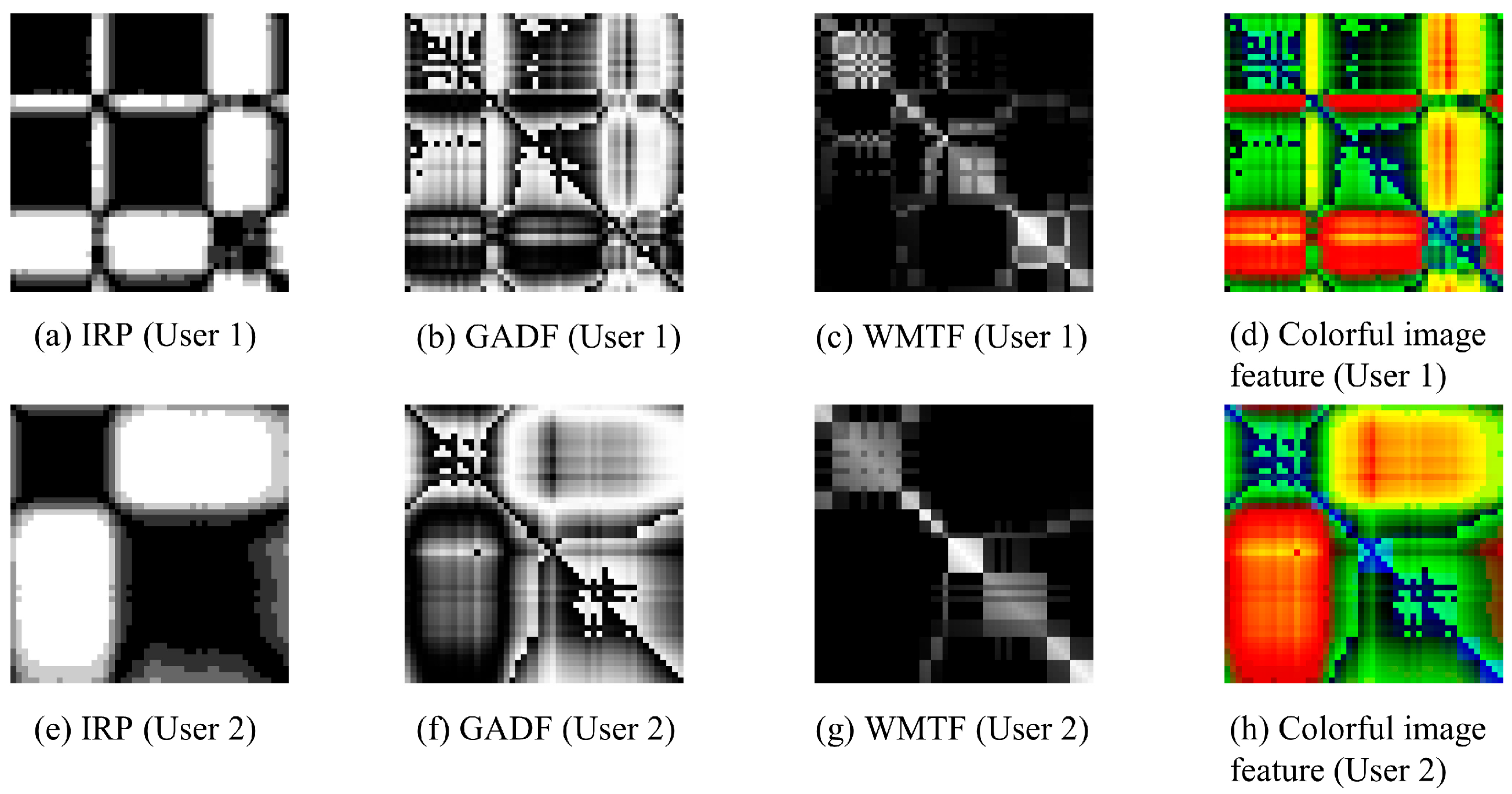
Therefore, this section constructs an improved recurrence plot (IRP) based on the typical daily electricity consumption curve, and further transforms the curve into two-dimensional grayscale images using the Gramian Angular Field (GAF) and Markov Transition Field (MTF) algorithms [20]. The three generated grayscale images are assigned to the red (R), green (G), and blue (B) channels of a single RGB image, respectively, forming a fused color image. This color image serves as an augmentation to the multivariate feature indicators, enriching the input representation for the subsequent evaluation model.
(1)
Improved Recurrence Plot
The Recurrence Plot (RP) is a visualization tool that detects and portrays the recurrence of states in a phase space, which can be used to analyze the dynamics of time series data such as daily electricity consumption curves. It achieves this by measuring similarities between different points in time, resulting in an image with symmetrical and block-like structures that reveal the repetitive and abrupt patterns within the curve. For a normalized typical electricity consumption curve l, the traditional RP is defined as a matrix R = [ri,j]∈{0,1}N×N, where:
r i , j = Θ ε l i * l j *
where ε is a distance threshold, and Θ(·) is the Heaviside step function, which outputs one if its argument is positive or zero, and zero otherwise.
However, traditional binary recurrence plots suffer from information loss during the simple thresholding process, which hinders further feature extraction and limits model performance improvements. To address these limitations, an Improved Recurrence Plot (IRP) method is proposed according to [21]. By introducing a discretization level η, the IRP extends the values of the recurrence plot elements beyond the binary state to η + 1 based on the distances between sampling points. This method effectively enriches the information contained within the image. Furthermore, it reduces the interference of data noise compared to using a distance matrix directly. It is calculated as follows:
r i , j = f l i * l j *
f d = 1 , d ε 1 η η d ε , d < ε
where ⌊·⌋ denotes the floor function.
(2)
Gramian Angular Field
The Gramian Angular Field (GAF) transforms a time series into an image by using polar coordinate mapping and sum/difference calculations. Specifically, the Gramian Angular Difference Field (GADF) encodes the angular differences of curve data, effectively preserving the trend and directionality between sequence data points.
The computation process for GADF is as follows. Firstly, to ensure that each point in the typical daily electricity consumption curve l can serve as an input for the cosine angle, the curve is scaled to the range [−1, 1]:
l ˜ i * = l i * min l * max l * min l * × 2 1
Subsequently, each point is then mapped to an angle ϕi in polar coordinates:
ϕ i = arccos l ˜ i *
The sine of the angular difference between every two points is then calculated to form the Gramian matrix G = [gi,j] ∈ [−1, 1]N×N:
g i , j = sin ϕ i ϕ j
(3)
Markov Transition Field
The Markov Transition Field (MTF) is a method for converting one-dimensional time series data into two-dimensional images by encoding the Markov transition probabilities between different states, effectively preserving the state evolution characteristics of the original time-domain data.
For a normalized typical daily electricity consumption curve l, this curve is divided into Q equal-frequency discrete quantile bins, where each element in the curve corresponds to a quantile qk (k ∈ [1, Q]). The first-order Markov transition frequencies between states are calculated to construct the transition probability matrix U = [uk,h] ∈ [0, 1]Q×Q:
u k , l = p l t + 1 q k | l t q h             = t = 1 N 1 I l t + 1 q k l t q h m = 1 Q t = 1 N 1 I l t + 1 q k l t q m
where uk,h represents the probability of a transition from quantile qk to quantile qh, and II(·) is an indicator function that equals one when the expression inside is true and zero otherwise.
For each pair of sampling points (i,j) in the curve, their transition probability is queried to construct the MTF matrix B = [bi,j]∈ [0, 1]N×N:
b i , j = u k , h
where yiqk and yjqh.
Given that electricity consumption curves typically exhibit strong local temporal dependencies, and patterns related to demand response potential are often concentrated within shorter time scales, this paper enhances the local information representation by weighting each element of the original MTF matrix based on the time interval. The weighted MTF (WMTF) matrix is computed as follows:
b i , j = exp γ i j 2 u k , h
where γ is a parameter that controls the decay rate of the weights, emphasizing more recent transitions over distant ones.
Figure 3 shows the image features constructed from the typical daily electricity consumption curves of the two users in Figure 2. The image features exhibit distinguishable characteristics for different users. The fused color image integrates these features with emphasis on their spatial composition, thereby enriching the information content and helping the model achieve better performance and training efficiency.

4. Demand Response Potential Evaluation Model Construction

4.1. Traditional Machine Learning Methods

Traditional machine learning methods focus on discovering statistical patterns in user electricity consumption data to evaluate demand response potential. Commonly used methods include Support Vector Machines (SVMs), XGBoost, and Random Forests (RFs).
For demand response potential evaluation, SVM aims to find an optimal regression hyperplane within a high-dimensional feature space. This is achieved by constructing a “margin” that maximizes the distance between different data points while minimizing prediction errors. The training process involves balancing model complexity and prediction error, often using kernel functions to address non-linear relationships effectively [22].
XGBoost is an ensemble learning method based on gradient boosting. It builds multiple weak prediction models (decision trees) sequentially, where each new tree fits the residuals of the current model, improving predictions through weighted accumulation. Specifically, XGBoost approximates loss functions using second-order Taylor expansion at each iteration and incorporates regularization terms to control model complexity, enhancing generalization and preventing overfitting [23].
Random Forest constructs numerous decision trees, trained on random subsets of the data and features, and aggregates their predictions via averaging or voting for the final output. This double randomness during training increases robustness and generalization. RF excels in providing stable ensemble structures and assessing feature importance [24].
Compared to deep learning, traditional machine learning methods, especially tree-based models (i.e., XGBoost and RF), are more suited for indicator features. SVM is adept at modeling smooth non-linear boundaries. XGBoost is proficient at capturing complex interactions and non-linear features. RF offers robust ensemble architecture and feature evaluation capabilities [25]. To leverage the predictive advantages of each model, this paper combines predictions from multiple models, as detailed in Section 4.3.

4.2. SE-ResNet Convolutional Neural Network

Compared to indicator features, images are sparse low-level features that require deep learning for deeper feature extraction. Convolutional neural networks (CNNs) leverage local perception, weight sharing, and hierarchical structures. These properties enable CNNs to efficiently extract spatial features from images. As a result, they have achieved remarkable success in computer vision and have given rise to many classic models. Among these, ResNet [26] introduces skip connections that allow the original input to bypass several convolutional layers and directly add to the output, effectively alleviating the vanishing gradient problem in deep networks. This allows networks to be trained deeper and more stably, significantly improving performance in tasks utilizing image features.
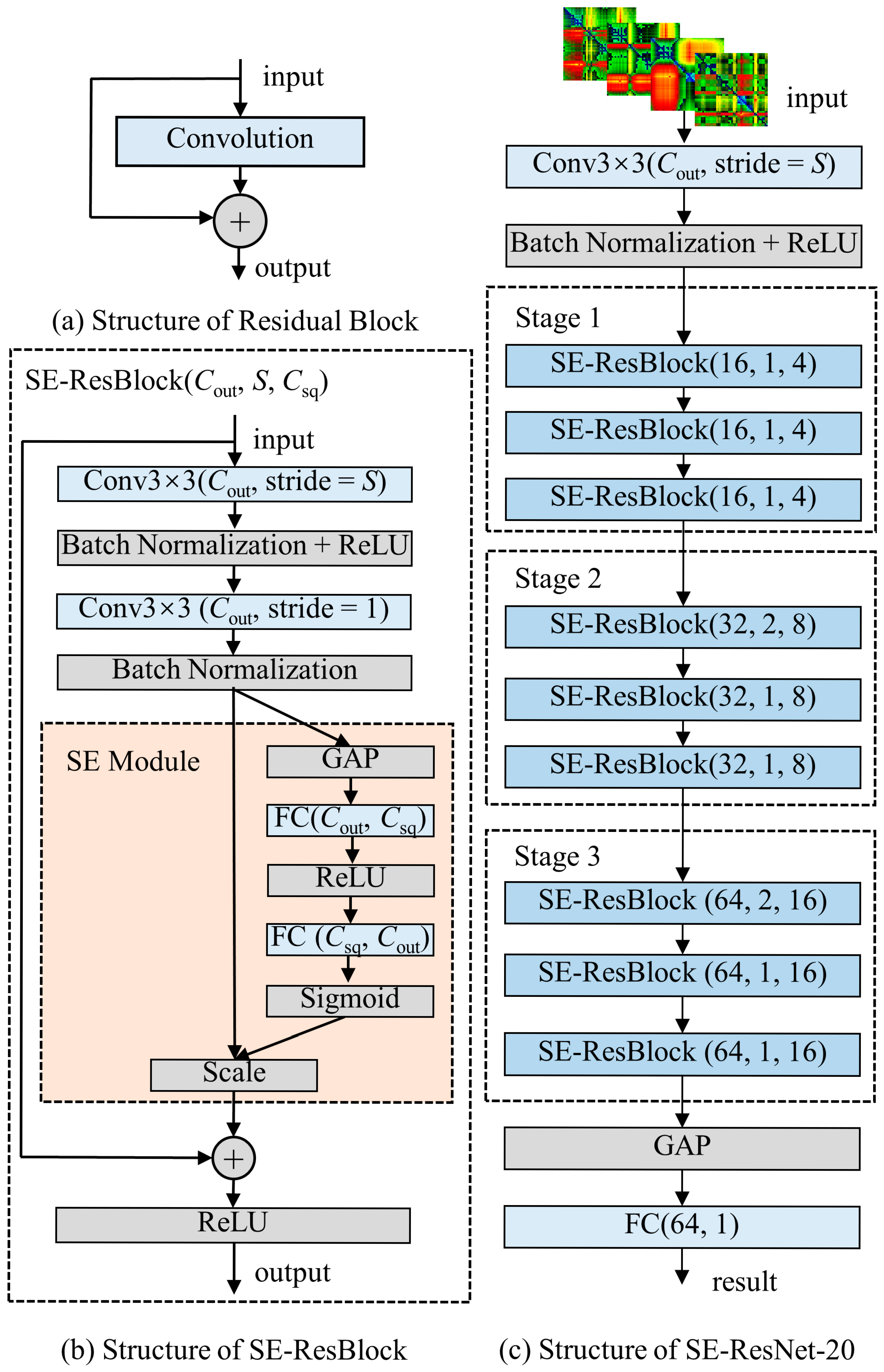
To further enhance the network’s ability to express important features, this paper incorporates the Squeeze-and-Excitation (SE) module [27], which uses the channel attention mechanism. As illustrated in Figure 4b, the SE module includes three main steps: squeeze, excitation, and reweight. During the squeeze step, the global average pooling (GAP) layer compresses information from each channel into a scalar, summarizing the global features of each channel. The excitation step uses two fully connected layers and an activation function to learn the importance weights of each channel. Specifically, the first fully connected layer reduces the number of channels to reduce computational cost, while the second restores it to the number of output channels. In the reweight step, each channel of the input feature map is multiplied by its corresponding channel weight to obtain the module’s output.
Considering the low-resolution image features used in the proposed method, the SE-ResNet-20 model is selected, originally designed for small-resolution images like those in CIFAR-10. Its concise network architecture makes it well-suited for extracting relevant characteristics from the image feature.
The structure of SE-ResNet-20, as shown in Figure 4c, consists of an initial convolutional layer, three stages, a GAP layer, and a fully connected layer. Each stage comprises three SE-ResBlocks, with the SE module placed between the convolutional layers and the skip connection operations. The first stage has 16 channels without changing resolution. In the second and third stages, the number of channels doubles, and down-sampling occurs in the first block of each stage.

4.3. Demand Response Potential Evaluation Model Based on Heterogeneous Base Stacking Mechanism

To integrate traditional machine learning methods with deep learning models for demand response potential evaluation, the Stacking mechanism is used in this paper. This method uses heterogeneous models as base learners and a decision tree as the meta learner to retrain on the evaluations produced by the base learners, aiming to achieve superior results.
Stacking [28] is an ensemble learning technique that involves training multiple heterogeneous base learners in parallel and then using a meta learner to combine their outputs into a stronger predictor. This method has shown success in many tasks in the electric power industry (e.g., distribution network loss prediction [29] and outage spatial distribution [30]). However, it remains underutilized in demand response potential evaluation. Within the stacking framework, diverse types of base models capture various features from the data, while the meta learner optimizes decision fusion based on their predictions. This combination effectively leverages the strengths of each model, reducing bias and variance, thereby enhancing overall prediction accuracy and generalization.
The proposed demand response potential evaluation model structure based on the heterogeneous base stacking mechanism is illustrated in Figure 5, and the list of features is shown in Table 1. For indicator features, SVM, XGBoost, and RF models are constructed and trained. For image features, the SE-ResNet-20 model described in Section 4.2 is used. These models serve as base learners, with a decision tree acting as the meta learner to form the complete demand response potential evaluation model.
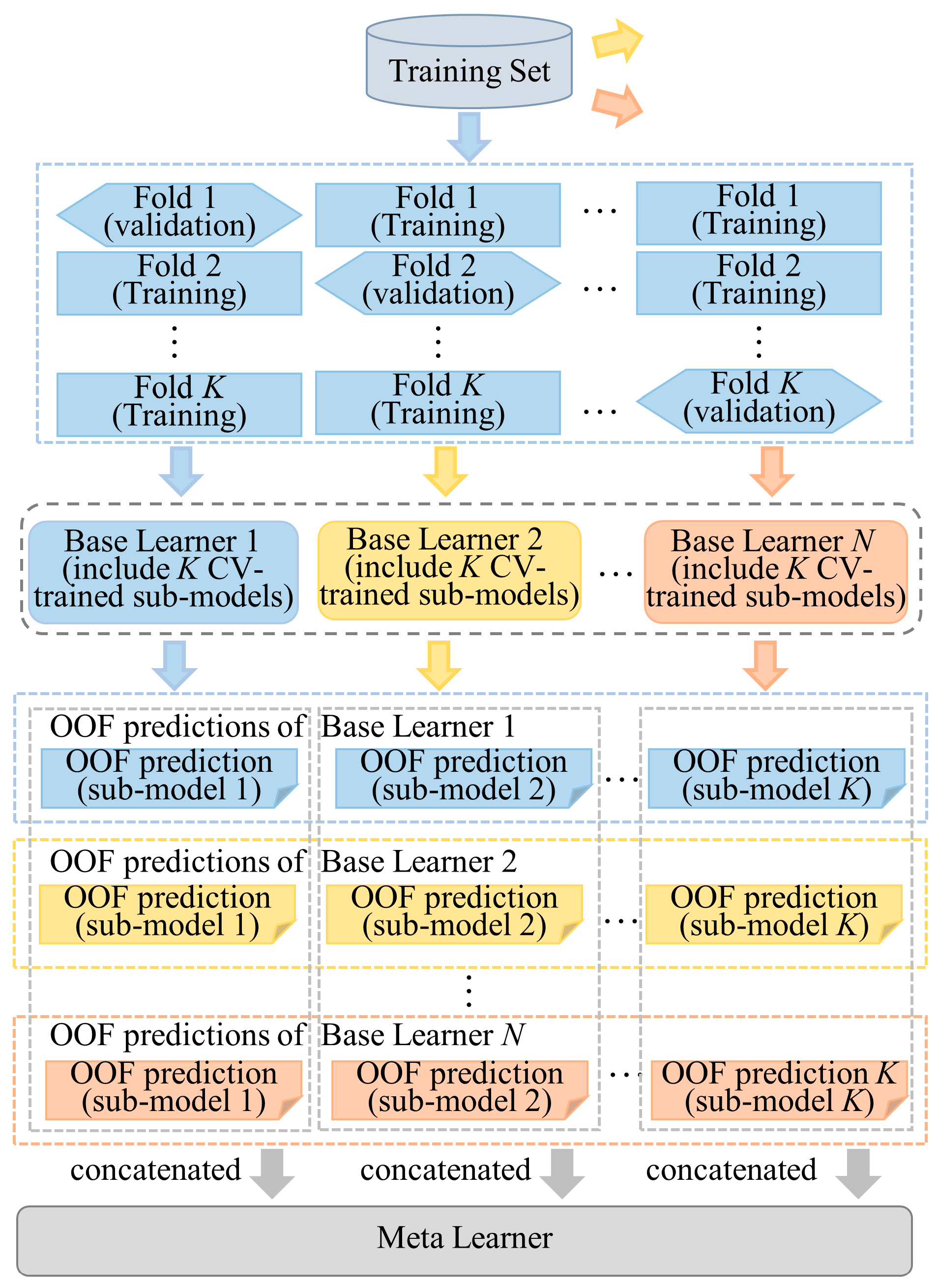
To mitigate the risk of overfitting, the model is generally trained using cross-validation (CV). As shown in Figure 6, The specific training and inference process of the Stacking model follows these steps, where different colored arrows and background colors are used to denote different base learners.
(1)
Split the training set into K folds.
(2)
Perform K rounds of training for each base learner. In each round, one fold is used as the validation set while the remaining K − 1 folds are used for training. Collect the predictions from the validation set after each training round to obtain the out-of-fold (OOF) predictions for the entire training set.
(3)
Repeat the above step for all base learners to gather their respective OOF predictions across the training set. These predictions are then concatenated and used as training samples for the meta learner.
(4)
During Inference, each base learner’s K sub-models trained during the cross-validation phase are used to make predictions on the test sample. The average of these predictions forms the final prediction for that base learner. The predictions from all base learners are then concatenated and fed into the meta learner, which outputs the final result.

5. Experimental Result and Discussion

5.1. Dataset and Label Calculation

To validate the effectiveness of the proposed method, this paper uses the Smart Meter Energy Consumption Data in London Households provided by UK Power Networks [31]. This dataset records the electricity consumption of 5567 London households from November 2011 to February 2014, with measurements taken at half-hour intervals. Among these households, 1103 users were on a time-of-use (TOU) pricing plan. The dataset records the periods during which users were exposed to high (67.20 pence/kWh), low (3.99 pence/kWh), and normal (11.76 pence/kWh) electricity prices. To avoid changes in user consumption patterns over an extended period, data from January 2013 to March 2013 for the TOU users are selected for analysis.
Temperature data corresponding to the London area during the same period is obtained from Visual Crossing [32]. Given that it only provides temperature data at hourly intervals, cubic spline interpolation [33] is used to interpolate the data to twice its original resolution, matching the half-hourly interval of the electricity consumption data.
Electricity consumption of individual users under high and low electricity prices reflects the demand response capacity. During high-price periods, if a user’s load falls below the baseline level observed under normal pricing, it indicates a response to the peak-shaving signal. The average reduction is taken as the user’s regulation capacity for peak shaving. Specifically, the regulation capacity at time i under high prices is calculated as:
C i high = 1 N i high × x i , j high X i high max 0 , l i x i , j high
where li is the sampled value at time i from the typical daily electricity consumption curve under normal pricing, obtained using the method described in Section 3.2. The X i high represents the set of load data at time i under high prices, x i , j high denotes the elements in X i high , and N i high is the number of elements in X i high .
To reduce misjudgments caused by uncertainties such as noise and short-term fluctuations, Equation (27) permits only data points below the typical daily electricity consumption curve to contribute positively, while those above the curve are uniformly assigned zero contribution. In addition, sample averaging is applied to the deviation at each time point to smooth out random noise.
Similarly, during low-price periods, if a user’s load exceeds the baseline level observed under normal pricing, it indicates a response to the valley-filling signal. The regulation capacity at time i under low prices is calculated as:
C i low = 1 N i low × x i , j low X i low max 0 , x i , j low l i
where X i low represents the set of load data at time i under low prices, x i , j low denotes the elements in X i low , and N i low is the number of elements in X i low .
The sum of regulation capacities across all periods is used as the label for demand response evaluation, which is used to train and validate the proposed method:
C high = i = 1 N C i high
C low = i = 1 N C i low

5.2. Experimental Setup

The experiments are conducted following these steps. First, the data is preprocessed according to Section 3.1, and electricity consumption data under high price, low price, and normal price periods are separated. The consumption data under normal pricing is used to extract indicator features and image features as described in the remaining part of Section 3. Demand response potential labels are calculated based on the consumption data under high and low pricing periods. The parameters for extracting image features are listed in Table 2.
The feature set is split into training and test sets using an 80%/20% ratio. Models are trained as described in Section 4. For deep learning models, the Mean Squared Error (MSE) loss function and the Adam optimizer are used, with a learning rate of 10−3. To prevent overfitting, training is stopped if the validation loss does not decrease for 10 consecutive epochs. For traditional machine learning models, grid search [34] is applied within each training fold to optimize hyperparameters and achieve better performance.
The experiments are conducted on a personal computer with an AMD Ryzen 9 5900 CPU (Advanced Micro Devices, Inc., Santa Clara, CA, USA) and 16 GB DDR4 RAM. The software environment includes Windows 10 Pro, Python 3.9, and PyTorch 1.12.0.

5.3. Metrics for Model Evaluation

Since demand response potential evaluation is a regression-like task, this paper employs the Mean Absolute Error (IMAE), Root Mean Squared Error (IRMSE), and Coefficient of Determination (R2) to comprehensively assess the experimental results. The IMAE measures the average deviation between predicted and actual values, IRMSE emphasizes larger prediction errors more heavily compared to MAE, and R2 assesses the model’s ability to explain the variance in the observed values. The formulas for these metrics are as follows:
I MAE = 1 N C × j = 1 N C C j C ^ j
I RMSE = 1 N C × j = 1 N C C j C ^ j 2
R 2 = 1 j = 1 N C C j C ^ j 2 j = 1 N C C j C ¯ 2
where Cj denotes the label for demand response evaluation of the j-th user sample calculated according to Section 5.1, C ^ j represents the demand response capacity predicted by the proposed method for the j-th user sample, NC is the total number of user samples, and C ¯ is the mean of the labels across NC user samples.

5.4. Comparative Experimental Results

To evaluate the effectiveness of the proposed demand response potential evaluation method compared with existing data-driven methods, its performance is compared with several alternative methods using different feature inputs and evaluation models. Specifically, the following methods are selected as baselines: For the typical daily electricity consumption curve (TECC), RNN and LSTM are used as evaluation models. For the typical daily electricity consumption image (TECI), LeNet-5, AlexNet, and the proposed SE-ResNet-20 are used as evaluation models. For indicator features for demand response (IFDR), MLP, SVM, and RF are used as evaluation models.
Table 3 and Table 4 present the experimental results for high-price (i.e., peak shaving) and low-price (i.e., valley filling) scenarios, respectively, including comparisons with the above methods. The best performance for each metric is highlighted in bold. The results show that the proposed method outperforms the common data-driven methods, demonstrating its ability to comprehensively capture and process information related to demand response potential, thereby improving the performance of demand response potential evaluation.
Further analysis of the comparative results reveals the impact of feature and model selection on demand response potential evaluation. Compared to one-dimensional TECC, two-dimensional TECI exhibits richer information related to demand response potential, which helps improve model learning performance, as reflected in the generally superior results in Table 3 and Table 4. Additionally, the proposed SE-ResNet-20 model performs better than the classical models (LeNet-5 and AlexNet) in the evaluation task. Compared to LeNet-5, SE-ResNet-20 uses residual connections to alleviate training difficulties in deep networks and embeds the SE module to enhance the modeling of key information related to demand response potential, thus improving performance. Compared to the deeper and larger AlexNet, the proposed model shows better structural adaptability when dealing with image features of only 48 × 48 resolution, enabling more efficient extraction of effective information and achieving better results.
From the experimental results of indicator features, it is evident that methods using indicator features significantly outperform those using TECC and TECI. This is because indicator features more intuitively reveal information related to demand response potential. Meanwhile, compared to the weighted average of historical daily electricity consumption curves in TECC, some indicators (e.g., ξ s p 2 b , ξ s v 2 b , σ s col ) retain more historical load information, effectively enhancing the evaluation of demand response potential. Furthermore, RF significantly outperforms other methods. Compared to MLP, RF improves R2 by 13.99% and 12.73% in high-price and low-price scenarios, respectively. This result highlights the superior adaptability of tree-based models in handling indicator features. Leveraging this advantage, RF is selected as one of the key base learners in the proposed Stacking method.
Notably, comparing Table 3 and Table 4 reveals that models perform better in high-price (peak shaving) scenarios but relatively poorly in low-price (valley filling) scenarios. This difference suggests variations in user response mechanisms. During high-price periods, users have a stronger motivation to reduce electricity consumption to reduce costs, leading to more regular behavior and a more significant correlation between load changes and price signals. This provides a clear and stable learning pattern for the model. In contrast, during low-price periods, despite the price incentive, users’ load-increasing behavior is often influenced by multiple factors such as living habits and appliance usage needs. As a result, the responses are more dispersed and uncertain, posing greater challenges for the model in learning and evaluating demand response potential.
Further analysis of different feature types shows that indicator features are subjected to a larger performance decrease in low-price scenarios, while image features exhibit better stability under the same conditions. This indicates that even though image features may have lower overall performance compared to indicator features, they have certain advantages in capturing the structural patterns of electricity consumption. After combining image features with indicator features, the model performance improves in both electricity price scenarios, with a more pronounced improvement observed in low-price conditions. Specifically, compared with the RF model using only indicator features, incorporating image features increases the R2 by 3.49% in high-price scenarios and by 12.54% in low-price scenarios. These results indicate that image features provide additional information that is particularly beneficial when user behavior becomes more irregular.
It should be noted that this comparison is conducted at the level of a single base learner (RF), aiming to highlight the intrinsic complementarity between image and indicator features. When the features are further integrated into the proposed stacking framework, their contributions are jointly leveraged by multiple base learners, which leads to more balanced and stable performance improvements, as discussed in Section 5.6. Overall, these results demonstrate that the fusion of image and indicator features is more effective than using a single type of feature, improving not only evaluation accuracy but also the applicability and robustness of the proposed method across different demand response scenarios.

5.5. Stacking Framework Performance Comparison

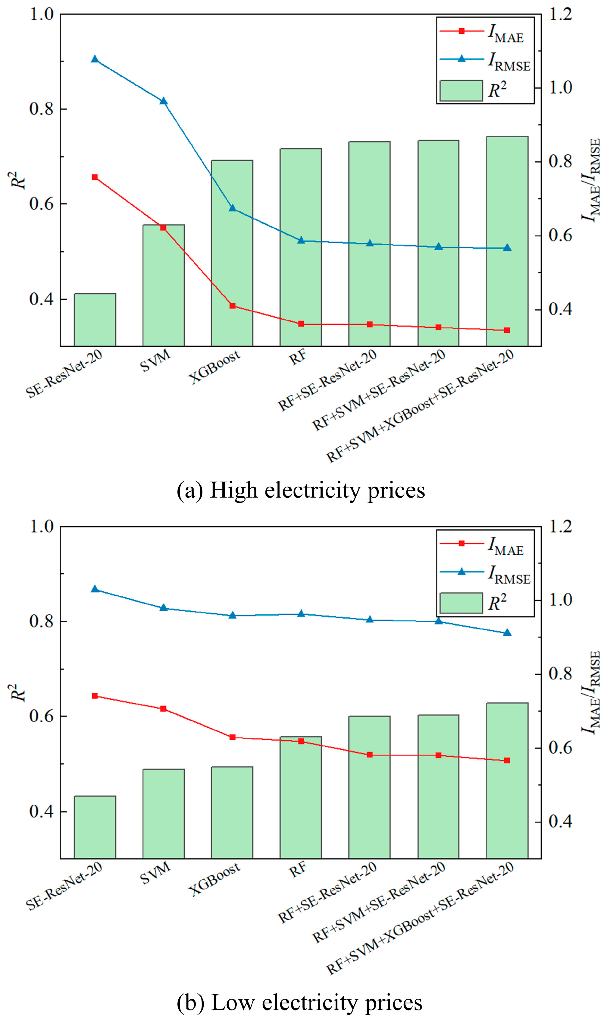
To evaluate the effectiveness of the Stacking mechanism in enhancing model performance, experiments are conducted starting with an RF base model. Other models are incrementally incorporated into the Stacking framework, and performance is tested at each stage. The changes in model performance are illustrated in Figure 7. The results show that the integrated model outperforms individual base learners across all performance metrics. Moreover, as more models are added to the integrated model, overall performance gradually improves. It is noteworthy that when incorporating SE-ResNet-20 based on image features into a baseline RF model that only uses indicator features, the greatest performance improvement is observed. This highlights the critical role of complementarity between different types of features and model architectures in achieving optimal performance.
The result underscores the significant advantages of using the Stacking mechanism for demand response potential evaluation. By integrating learners with varying structures and modeling mechanisms, the Stacking mechanism effectively captures the sensitivity and focus of different models towards various aspects of data distribution, thereby enhancing the expressiveness of feature information and overall performance. Additionally, the meta learner, through relearning from the outputs of base models, adaptively assigns weights to these models. This not only maintains flexibility but also mitigates issues like overfitting or underfitting that might arise from relying on a single model.
Furthermore, the Stacking mechanism provides a means to combine indicator and image features, expanding the informational scope of the model and improving the reliability of demand response potential evaluation. This fusion strategy leverages the strengths of both feature types, ensuring a more robust and accurate evaluation by capturing comprehensive patterns and nuances within the data. Consequently, the Stacking mechanism proves to be an effective solution for enhancing the evaluation capabilities and generalization performance in demand response potential evaluations.

5.6. Ablation Studies

To verify the contribution of each feature type to the performance of the proposed demand response potential evaluation method, ablation studies are conducted by controlling input features. The settings of each experimental group are listed in Table 5.
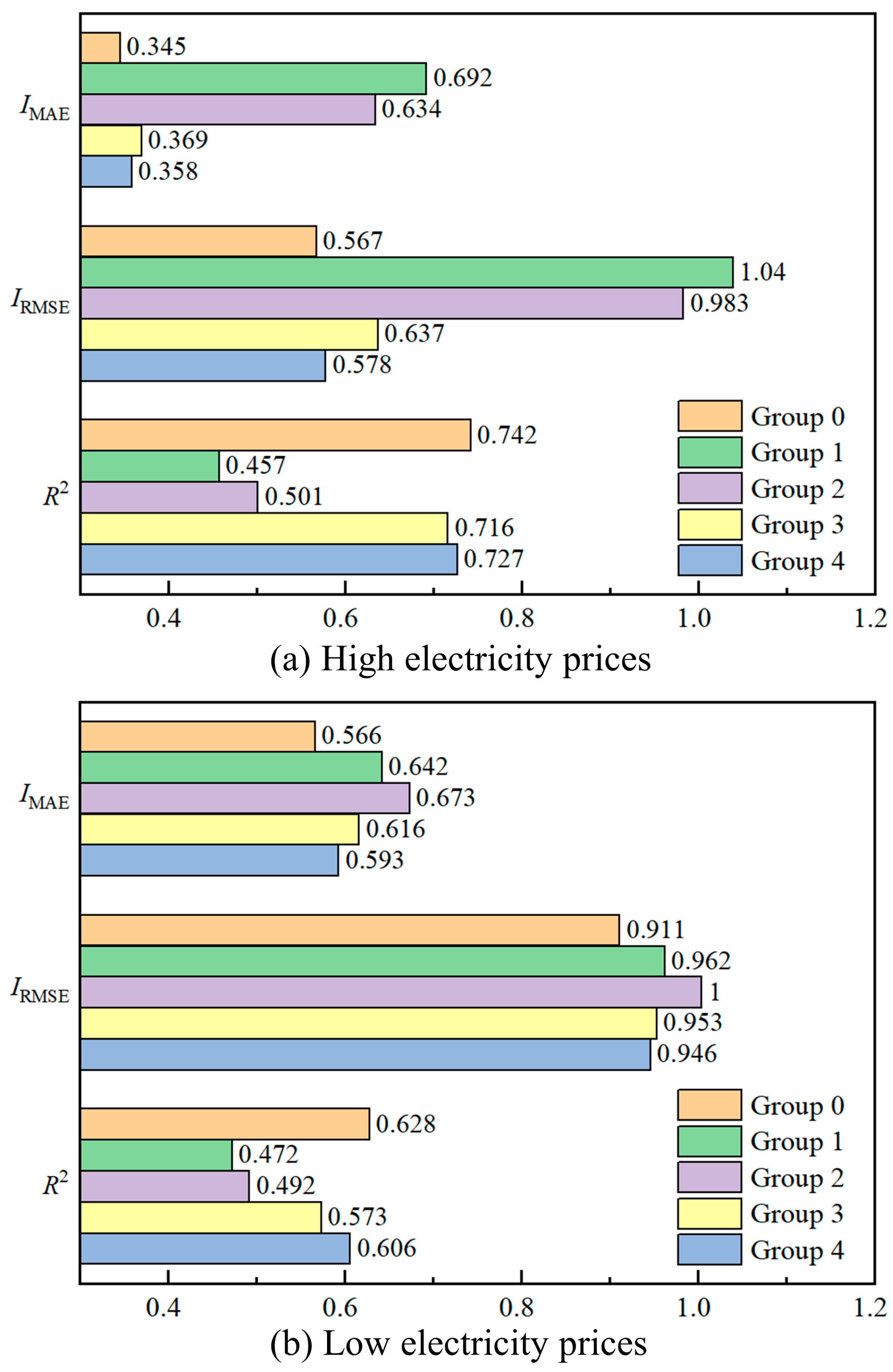
Figure 8 presents the results of the ablation experiments. In Group 1, where load shape features are removed, the R2 decreases from 0.742 to 0.457 in the high-price scenario, and the MAE increases from 0.345 to 0.692. This indicates that intra-day load structure and overall load level are core information sources for the model to evaluate peak shaving potential. In Group 2, the removal of load variability features leads to a significant decrease in R2 from 0.628 to 0.492 under the low-price scenario, highlighting the critical role of volatility in characterizing user flexibility and evaluating the potential of valley filling. Group 3, which excludes load correlation features, also showed a decline in overall model performance, confirming the significant value of external contextual factors in describing user load variations. In Group 4, removing image features results in a moderate but consistent performance degradation across both electricity price scenarios. Although the impact is less pronounced than that of some indicator features, image features provide complementary structural information from load profiles, contributing positively to the overall performance and stability of the proposed method, as analyzed in Section 5.4. These results collectively indicate that all proposed feature types contribute positively to model performance and exhibit strong complementarity.
Furthermore, the importance of different features varies across pricing scenarios. In the high-price (peak shaving) scenario, Group 1 are subjected to the most significant performance decrease, suggesting that underprice incentives, users tend to reduce consumption in a more regular and predictable manner, making load level and structural features particularly crucial.
In contrast, in the low-price (valley filling) scenario, Group 2 showed the largest performance decline, reflecting that user behavior in increasing consumption is influenced by multiple factors beyond price, thus increasing the importance of variability features. Additionally, comparing Group 0 and Group 3, the load correlation features contributed more in the low-price scenario, with an R2 improvement of 9.60%, which is significantly higher than the 3.63% observed in the high-price scenario.
In summary, the integration of image features with multiple types of indicator features significantly enhances both the evaluation performance and scenario adaptability of the model. This validates the broad applicability and practical value of the proposed method across diverse demand response scenarios.

6. Conclusions

This paper focuses on mining the relationship between user electricity consumption data and demand response potential, and on achieving effective demand response potential evaluation through a data-driven method, based on multivariate heterogeneous features and the Stacking mechanism. In terms of feature extraction, multidimensional indicator features are extracted from the shape, variability, and correlation aspects of electricity consumption data to explicitly express information relevant to demand response potential. Furthermore, color image features are constructed based on typical daily electricity consumption curves of users to explore deeper characteristics. For the construction of the evaluation model, the Stacking mechanism from ensemble learning is introduced, training multiple traditional machine learning algorithms alongside an SE-ResNet-20 model as base learners, before constructing a meta learner to learn from the results of the base learners. This method fully leverages the advantages of different models to achieve effective integration of multivariate heterogeneous features. Experimental results on the Smart Meter Energy Consumption Data in London Households demonstrate that the proposed method outperforms common data-driven methods. Extended experiments separately verify the selection of multivariate heterogeneous features and the enhancement of model performance brought by the Stacking mechanism.
Future work will focus on the following aspects:
(1)
Further exploration of intrinsic load characteristics and features related to external influencing factors will be conducted. Based on these features, preprocessing strategies will be optimized, and systematic feature evaluation and selection will be performed to identify the most suitable input features for different heterogeneous models.
(2)
Lightweight image feature representations or adaptive feature activation mechanisms will be investigated to reduce the computational burden of the models.
(3)
The proposed method will be further validated and analyzed in a wider range of real-world scenarios, and insights gained from these results will be used to continuously refine the framework and improve its overall performance.

Author Contributions

Methodology, C.G., Z.X. and W.X.; Software, C.G. and R.C.; Validation, X.W. and T.Y.; Formal analysis, H.Z.; Investigation, R.C., J.Z. and X.W.; Resources, J.Z. and T.Y.; Data curation, Z.X.; Writing—original draft, C.G., Z.X. and R.C.; Visualization, H.Z.; Supervision, J.Z. and W.X.; Project administration, Z.X. and R.C.; Funding acquisition, C.G. All authors have read and agreed to the published version of the manuscript.

Funding

This research was supported by the China Southern Power Grid Corporation Technology Project (037700KC23120014, GDKJXM20231346).

Data Availability Statement

The original contributions presented in this study are included in the article. Further inquiries can be directed to the corresponding author.

Conflicts of Interest

Authors Chong Gao, Zhiheng Xu, Ran Cheng, Junxiao Zhang and Xinghang Weng were employed by the company Power System Planning Research Center of Guangdong Power Grid Co., Ltd. The remaining authors declare that the research was conducted in the absence of any commercial or financial relationships that could be construed as a potential conflict of interest.

References

  1. Prasad, M.B.; Ganesh, P.; Kumar, K.V.; Mohanarao, P.A.; Swathi, A.; Manoj, V. Renewable Energy Integration in Modern Power Systems: Challenges and Opportunities. In E3S Web of Conferences; EDP Sciences: Les Ulis, France, 2024; Volume 591, p. 03002. [Google Scholar]
  2. Pinson, P.; Madsen, H. Benefits and challenges of electrical demand response: A critical review. Renew. Sustain. Energy Rev. 2014, 39, 686–699. [Google Scholar] [CrossRef]
  3. Aghaei, J.; Alizadeh, M.I. Demand response in smart electricity grids equipped with renewable energy sources: A review. Renew. Sustain. Energy Rev. 2013, 18, 64–72. [Google Scholar] [CrossRef]
  4. Zhang, Y.; Li, Y.; Cheng, B.; Liu, W.; Zhang, H.; Kong, X. Data-Driven Demand Response Potential Assessment and Adjustable Load Optimization Scheduling. In Proceedings of the 2024 IEEE 25th China Conference on System Simulation Technology and its Application (CCSSTA), Tianjin, China, 21–23 July 2024; pp. 863–868. [Google Scholar] [CrossRef]
  5. Wang, B.B.; Xu, P.; Wang, X.Y. Distributionally robust modeling of demand response and its large-scale potential deduction method. Autom. Electr. Power Syst. 2022, 46, 33–41. [Google Scholar] [CrossRef]
  6. Luo, J.M.; Wen, Z.C.; Dong, W.J. Model of integrated demand response potential based on portrait of residential users. Renew. Energy Resour. 2020, 38, 1407–1414. [Google Scholar] [CrossRef]
  7. Li, Z.Y.; Ai, Q. Demand response estimation method of electricity consumption for residential customer under time of use price. Electr. Power Autom. Equip. 2023, 43, 121–127. [Google Scholar] [CrossRef]
  8. Wang, S.J.; Pan, D.B. Research on emergency management capability evaluation method of natural disasters based on set pair analysis. J. Nat. Disasters 2023, 32, 104–116. [Google Scholar] [CrossRef]
  9. Qi, N.; Cheng, L.; Xu, H.; Wang, Z.; Zhou, X. Practical Demand Response Potential Evaluation of Air-Conditioning Loads for Aggregated Customers. Energy Rep. 2020, 6, 71–81. [Google Scholar] [CrossRef]
  10. Xu, W.; Shao, W.; Ma, Z.; Xu, Z.; Wang, N. Dynamic Optimization of Charging Strategies for EV Parking Lot under Real-Time Pricing. In Proceedings of the 2016 35th Chinese control conference (CCC), Chengdu, China, 27–29 July 2016; pp. 2703–2709. [Google Scholar]
  11. Karapetyan, A.; Khonji, M.; Chau, S.C.K.; Elbassioni, K.; Zeineldin, H.; El-Fouly, T.H.; Al-Durra, A. A Competitive Scheduling Algorithm for Online Demand Response in Islanded Microgrids. IEEE Trans. Power Syst. 2021, 36, 3430–3440. [Google Scholar] [CrossRef]
  12. Liang, H.; Ma, J. Data-Driven Resource Planning for Virtual Power Plant Integrating Demand Response Customer Selection and Storage. IEEE Trans. Ind. Inform. 2022, 18, 1833–1844. [Google Scholar] [CrossRef]
  13. Samad, T.; Koch, E.; Stluka, P. Automated Demand Response for Smart Buildings and Microgrids: The State of the Practice and Research Challenges. Proc. IEEE 2016, 104, 726–744. [Google Scholar] [CrossRef]
  14. Zheng, S.; Sun, Y.; Qi, B.; Li, B. Incentive-Based Integrated Demand Response Considering S&C Effect in Demand Side with Incomplete Information. IEEE Trans. Smart Grid 2022, 13, 4465–4482. [Google Scholar] [CrossRef]
  15. Song, Z.; Shi, J.; Li, S.; Chen, Z.; Jiao, F.; Yang, W.; Zhang, Z. Data-driven and physical model-based evaluation method for the achievable demand response potential of residential consumers’ air conditioning loads. Appl. Energy 2022, 307, 118017. [Google Scholar] [CrossRef]
  16. Adika, C.O.; Wang, L. Smart charging and appliance scheduling approaches to demand side management. Int. J. Electr. Power Energy Syst. 2014, 57, 232–240. [Google Scholar] [CrossRef]
  17. Pallonetto, F.; De Rosa, M.; Milano, F.; Finn, D.P. Demand response algorithms for smart-grid ready residential buildings using machine learning models. Appl. Energy 2019, 239, 1265–1282. [Google Scholar] [CrossRef]
  18. Rdusseeun, L.; Kaufman, P. Clustering by means of medoids. In Proceedings of the Statistical Data Analysis Based on the L1 Norm Conference, Neuchatel, Switzerland, 31 August–4 September 1987; Volume 31, p. 28. [Google Scholar]
  19. Nigro, L.; Fränti, P. Two medoid-based algorithms for clustering sets. Algorithms 2023, 16, 349. [Google Scholar] [CrossRef]
  20. Wang, Z.; Oates, T. Imaging time-series to improve classification and imputation. In Proceedings of the 24th International Conference on Artificial Intelligence, Buenos Aires, Argentina, 25–31 July 2015; AAAI Press: Washington, DC, USA, 2015; pp. 3939–3945. [Google Scholar]
  21. Faustine, A.; Pereira, L. Improved appliance classification in non-intrusive load monitoring using weighted recurrence graph and convolutional neural networks. Energies 2020, 13, 3374. [Google Scholar] [CrossRef]
  22. Damousis, I.G.; Bakirtzis, A.G.; Dokopoulos, P.S. A solution to the unit-commitment problem using integer-coded genetic algorithm. IEEE Trans. Power Syst. 2004, 19, 1165–1172. [Google Scholar] [CrossRef]
  23. Zhao, Q.; Xiang, W.; Huang, B.; Wang, J.; Fang, J. Optimised extreme gradient boosting model for short term electric load demand forecasting of regional grid system. Sci. Rep. 2022, 12, 19282. [Google Scholar] [CrossRef]
  24. Bai, Z.; Liu, Q.; Gong, L.; Lei, J. Application of a mid-/low-temperature solar thermochemical technology in the distributed energy system with cooling, heating and power production. Appl. Energy 2019, 253, 113491. [Google Scholar] [CrossRef]
  25. Jiang, H.; Lu, N.; Qin, J.; Tang, W.; Yao, L. A deep learning algorithm to estimate hourly global solar radiation from geostationary satellite data. Renew. Sustain. Energy Rev. 2019, 114, 109327. [Google Scholar] [CrossRef]
  26. He, K.; Zhang, X.; Ren, S.; Sun, J. Deep Residual Learning for Image Recognition. In Proceedings of the IEEE Conference on Computer Vision and Pattern Recognition (CVPR), Las Vegas, NV, USA, 27–30 June 2016; pp. 770–778. [Google Scholar]
  27. Hu, J.; Shen, L.; Sun, G. Squeeze-and-Excitation Networks. In Proceedings of the IEEE Conference on Computer Vision and Pattern Recognition (CVPR), Salt Lake City, UT, USA, 18–23 June 2018; pp. 7132–7141. [Google Scholar]
  28. Zhou, Z. Ensemble Methods: Foundations and Algorithms; Taylor & Francis: Abingdon, UK, 2012. [Google Scholar]
  29. Deng, W.; Guo, Y.; Li, Y.; Zhu, L.; Liu, D. Power losses prediction based on feature selection and Stacking integrated learning. Power Syst. Prot. Control 2020, 48, 108–115. [Google Scholar] [CrossRef]
  30. Hou, H.; Chen, X.; Li, M.; Zhu, L.; Huang, Y.; Zhu, S. A space prediction method for power outage in a typhoon disaster based on a Stacking integrated structure. Power Syst. Prot. Control 2022, 50, 76–84. [Google Scholar] [CrossRef]
  31. UK Data Service. Low Carbon London Project Data. Available online: https://data.london.gov.uk/dataset/smartmeter-energy-use-data-in-london-households (accessed on 24 December 2025).
  32. Weather Data services. Weather History for London. Available online: https://www.visualcrossing.com/weather/weather-data-services (accessed on 24 December 2025).
  33. Sauer, T. Numerical Analysis, 3rd ed.; Pearson: Boston, MA, USA, 2012. [Google Scholar]
  34. Hastie, T.; Tibshirani, R.; Friedman, J. The Elements of Statistical Learning: Data Mining, Inference, and Prediction, 2nd ed.; Springer: New York, NY, USA, 2009. [Google Scholar]
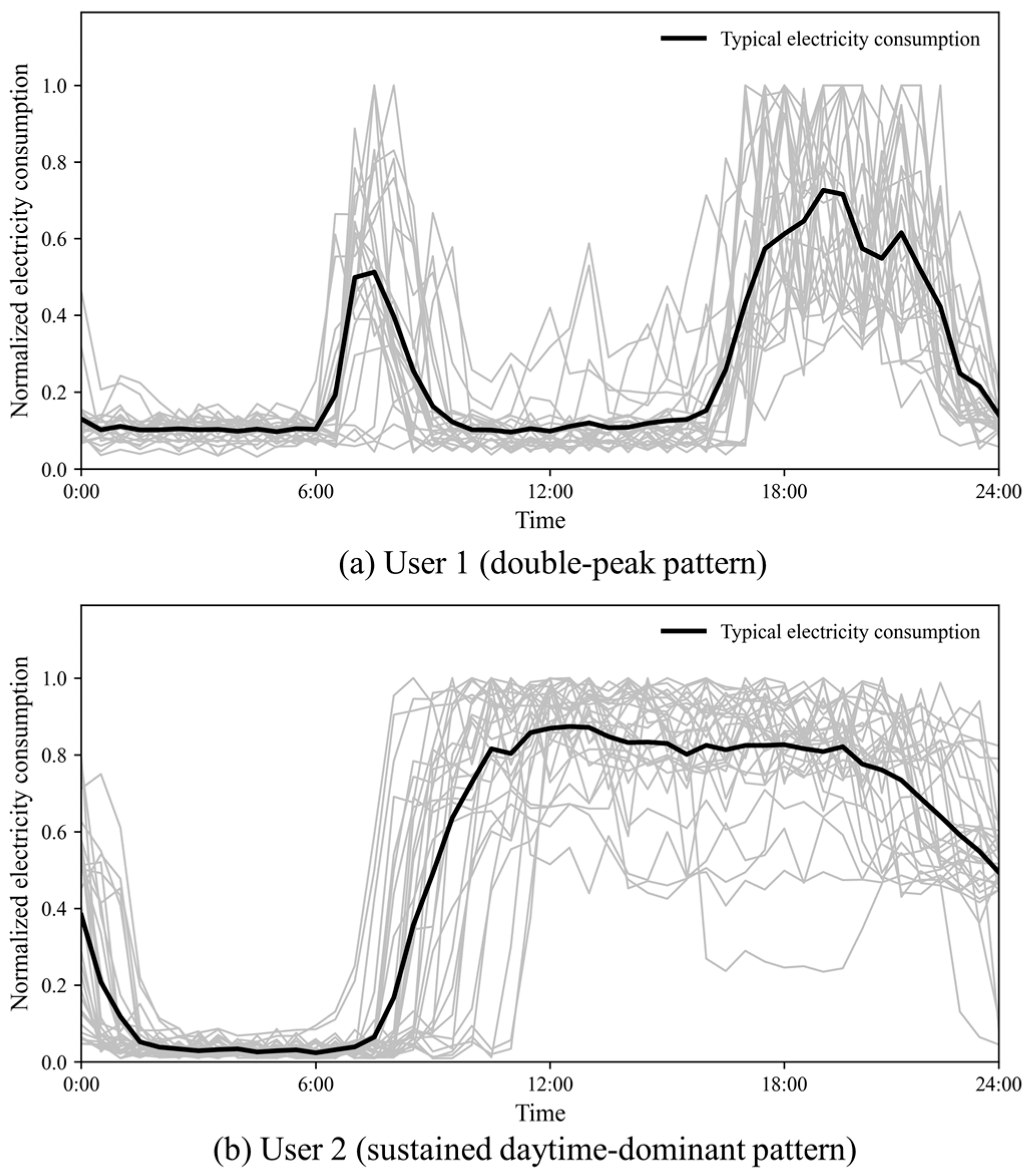
Figure 2. Typical daily electricity consumption curves.
Energies 19 00194 g002
Figure 3. Examples of proposed image features.
Energies 19 00194 g003
Figure 4. Structure of the modules and network of SE-ResNet-20.
Energies 19 00194 g004
Figure 5. Structure of the proposed demand response potential evaluation model.
Energies 19 00194 g005
Figure 6. Schematic of the Stacking model training process.
Energies 19 00194 g006
Figure 7. Comparison of Stacking models.
Energies 19 00194 g007
Figure 8. Results of ablation experiments.
Energies 19 00194 g008
Table 1. List of features.
Target ModelFeature CategoryFeature
Subcategory
Symbol/
Abbreviation
Description
SE-ResNet-20Image feature/IRPImproved Recurrence Plot
GADFGramian Angular Difference Field
WMTFWeighted Markov Transition Field
SVM
RF
XGBoost
Indicator featureLoad Shape FeaturePAverage power over the entire day of the typical daily electricity consumption curve (TECC)
PsAverage power over each period of the TECC
ξp2mPeak-to-average ratio of the TECC
ξp2vNormalized peak-to-valley difference of the TECC
ξ s p 2 b The upper deviation magnitude from the TECC for each period
ξ s v 2 b The lower deviation magnitude from the TECC for each period
Load Variability Feature σ s row Variability within daily electricity consumption for each period
σ s col Variability at identical time points across different days for each period
Load Correlation FeaturektSpearman correlation coefficient between the TECC and temperature
khSpearman correlation coefficient between the TECC of weekdays and holidays
Table 2. Parameters for extracting image features.
ParameterValue
GeneralImage resolution48 × 48
IRPDistance threshold ε0.5
Discretization level η5
GADF--
WMTFNumber of quantile bins Q8
Weight attenuation coefficient γ0.05
Table 3. Results of demand respond potential evaluation under high prices.
FeatureModelIMAEIRMSER2
TECCRNN0.7951.2040.339
LSTM0.8231.1060.341
TECILeNet-50.7811.2250.298
AlexNet0.7661.0950.375
SE-ResNet-200.7581.0770.412
IFDRMLP0.630.9380.629
SVM0.6210.9640.556
RF0.3620.5870.717
TECI + IFDR
(proposed)
Stacking (proposed)0.3450.5670.742
Table 4. Results of demand response potential evaluation under low prices.
FeatureModelIMAEIRMSER2
TECCRNN0.8871.2250.308
LSTM0.9081.3030.256
TECILeNet-50.8011.1030.31
AlexNet0.7791.0980.366
SE-ResNet-200.7411.0290.433
IFDRMLP0.6890.9890.495
SVM0.7070.9790.489
RF0.6190.9640.558
TECI + IFDR (proposed)Stacking (proposed)0.5660.9110.628
Table 5. Settings for ablation studies.
Experimental GroupDescription
Group 0Adopt all the proposed features.
Group 1Remove load shape features.
Group 2Remove load variability features.
Group 3Remove load correlation features.
Group 4Remove image features.
Disclaimer/Publisher’s Note: The statements, opinions and data contained in all publications are solely those of the individual author(s) and contributor(s) and not of MDPI and/or the editor(s). MDPI and/or the editor(s) disclaim responsibility for any injury to people or property resulting from any ideas, methods, instructions or products referred to in the content.