Abstract
This research aimed to ascertain the ZIP (constant impedance, constant current, and constant power) coefficients and Conservation of Voltage Reduction factor (CVRf) for residential appliances as well as for the residential network feeders in Malaysia through measurement and simulation analysis. The required power data were obtained through varying the supply voltage from 250 V to 215 V with a 5 V reduction. The appliances’ components were identified using the ZIP coefficients solved with the Sequential Least Squares Programming optimizer in Python (Spyder 5.5.4). The CVRf for residential appliances was determined using the well-established voltage and power correlation analysis. The study’s findings demonstrate a strong association between the appliance load composition determined by the ZIP load model and CVRf. This paper’s primary contribution is a comprehensive analysis conducted using the ZIP and CVR techniques to ascertain each appliance’s load composition. Based on the findings of this study, a classification is developed and extended to include a range of findings from other published studies in which the conclusion is consistent. Moreover, the CVRf value for one residence corresponds to a residential substation CVRf which is further validated via bottom-up load model analysis. The main contribution of this paper is to categorize residential appliances based on constant impedance, constant current, and constant power through the ZIP load model and the CVRf. Additionally, this CVR analysis is the pioneer study in Malaysia; thus, it is crucial to develop a systematic approach for identifying and classifying household devices according to their electrical characteristics. Load categorization provides the fundamental understanding about an appliance to determine its behavior towards a change in voltage, thus establishing cost savings and energy management in a home.
1. Introduction
Optimizing energy management in residential settings necessitates understanding how appliances behave under varying electrical conditions. Residential appliances can be categorized as constant impedance, constant current, or constant power devices, each with distinct energy consumption characteristics [1]. For instance, constant impedance devices have straightforward consumption patterns, while constant power appliances enable consistent efficiency improvements. Constant current devices adjust their power draw corresponding to the voltage variation [2]. This categorization plays a critical role in selecting energy-efficient appliances, stabilizing energy demand, and implementing targeted energy-saving strategies, thereby reducing electricity costs and improving load flow and stability assessments.
A key framework for analyzing load behavior is the ZIP model, which represents constant impedance (Z), constant current (I), and constant power (P) loads. The ZIP model characterizes the voltage dependency of appliances, with its coefficients indicating the proportional contribution of each component. This model provides a mathematical basis for predicting the load behavior under varying voltage and frequency conditions, making it essential for power system analysis and energy management [3,4,5]. Furthermore, the ZIP load model contributes significantly to voltage stability assessments, helping to evaluate how appliances influence overall system reliability.
The Conservation Voltage Reduction (CVR) technique, widely used for peak load reduction and energy savings, thus highlights the importance of understanding load behavior [6]. CVR reduces endpoint voltages in a controlled manner, decreasing the power consumption of resistive and constant current loads without adversely affecting consumers [7,8]. Assessing appliance behavior under CVR conditions enables utilities to maximize energy savings while ensuring system stability [9].
Despite the extensive studies on ZIP load coefficients, there is a lack of systematic categorization of residential appliances as constant impedance, current, or power types. This study addresses this gap by categorizing residential appliances based on ZIP load analysis and incorporating the existing published model results. The outcome obtained is strengthened by performing percentage normalization for the categorization established. By understanding the energy consumption patterns of appliances across different voltage levels, this research provides actionable insights for optimizing energy management, improving load forecasting, and enabling informed decision making.
The main contribution of this paper is that it provides the specific load model, CVRf, and load categorization for residential appliances in Malaysia. A load model is developed and the impact of the voltage reduction on the power consumption of each appliance is observed. Most research introduces one constraint for the ZIP analysis which is that the total ZIP load coefficients must sum to 1; however, an additional constraint is introduced in this study which is to only allow positive values for the ZIP load coefficients which is between 0 and 1. This approach was chosen as it more accurately reflects the appliance usage in a Malaysian residential scenario. The ZIP and CVRf analysis results were used to determine the appliance classification. Based on the findings of this investigation, a classification is developed, and it is extended to include a range of results from various published journals, where the conclusion is consistent with this analysis. In addition, one residence CVRf is established and verified with a residential substation CVRf which is further validated with a bottom-up load model simulation. This voltage reduction is a pioneering study that can support Malaysia’s progress in developing smart grids and smart cities. These foundational methods establish a strong base for future innovative research in energy management and smart grid optimization.
This paper comprises Section 1 as the general background information, Section 2 as comprehensive coverage via a literature review, Section 3 as the methodology of the study that includes the data collection for the residential appliances, Section 4 as the comprehensive results and discussion from the analysis performed on CVR and the categorization of residential appliances, and Section 5 as the conclusion derived from this study.
2. Literature Review
Non-intrusive Appliance Load Monitoring (NILM) leverages advanced signal processing and machine learning techniques to analyze and classify electrical loads, offering significant advancements in energy management. Recent methods highlight its potential; a phase-diagram-based technique integrated with machine learning achieved over 98% accuracy, outperforming the traditional approaches for practical energy management [10]. An Auto Regressive Moving Average with eXternal inputs (ARMAX) model-based method eliminates the need for prior appliance knowledge, simplifying the implementation for energy metering and billing [11]. Weighted recurrence graph (WRG) features combined with convolutional neural networks (CNNs) enhanced the appliance classification accuracy, achieving a Matthews correlation coefficient of up to 1.0 on datasets like Controlled On/Off Loads Library (COOLL) [12]. A cross-correlation-based methodology with machine learning and dimensionality reduction facilitated the real-time load classification of microcontrollers, improving the energy efficiency as achieved in [13]. While NILM is cost-effective and scalable, challenges include achieving accurate disaggregation in homes with many appliances or overlapping energy patterns, which can be complex, and processing large volumes of data in real time can be demanding. However, these studies do not explicitly categorize appliances based on specific load types, such as constant impedance, constant current, or constant power loads, which is crucial for CVR analysis as discussed in this paper. As Malaysia grows in its implementation of smart cities and smart meters, these foundational methods provide a base for future progressive studies in energy management and smart grid optimization.
On the contrary, load modeling refers to the mathematical representation of the relationship between power and voltage at a load bus which is essential for power system analysis, planning, and control [14]. A load model can be categorized into two main types, i.e., static models, which express active and reactive power as functions of voltage and frequency, and dynamic models, which account for the time-varying behaviors of loads. A load model analysis was performed by [15] developing time and voltage domain load models for appliance-level grid edge simulation and control. The methodology involves the experimental measurements of real and reactive power, current, and voltage over extended periods of time. The accuracy of the proposed load models and system identification algorithms were evaluated by testing 19 appliances that were limited to lights, fans, mini refrigerators, and space heaters. The findings of the research indicate that several appliance types exhibit a time-invariant voltage–power relationship and can be accurately modeled with the traditional ZIP model. The paper [16] employs several methods for load modeling, primarily focusing on the Automated Load Modeling Tool (ALMT) at the grid level. The ALMT is utilized to enhance the efficiency of load modeling by processing real-time data collected from the power system. Additionally, the Least Square Error (LSE) method is applied for parameter estimation, allowing for the comparison of simulated load models with actual recorded data. The method used for load modeling in [5] involves measuring the active and reactive power consumption of 18 household appliances at varying voltages from 100 V to 240 V in 10 V increments. The collected data are then utilized to calculate ZIP coefficients using the Least Square Algorithm, which represent the relationship between the power consumption and voltage for each appliance. Subsequently, these ZIP coefficients are applied alongside an assumed appliance usage pattern to generate daily active and reactive power demand profiles. The accuracy of the ZIP model is validated by comparing the generated profiles with actual measurement data.
The impact of CVR can be assessed using the Conservation Voltage Reduction Factor (CVRf) with the percentage reduction in power divided by the percentage reduction in voltage. The study in [17] explores peak load management strategies for distribution networks which include CVR and Dynamic Thermal Rating (DTR). It finds that implementing CVR alone results in a 38.45% cost reduction during peak hours, allowing for more loads to be supplied and enhancing the voltage reduction potential of the network. Higher savings were observed through implementing CVR and DTR. However, the study emphasizes that a smart grid environment is essential for the successful implementation of CVR and DTR, which may limit their applicability in conventional distribution networks. In [18], the method used to determine CVR involves both theoretical analysis and experimental verification. The researchers developed a criterion to assess the effectiveness of CVR by analyzing the relationship between the efficiency of refrigeration loads and their energy intake during reduced voltage operation. The voltage was systematically reduced, within a range of 3% to 7%. The study combines analytical models with experimental data to validate the energy savings achieved through CVR. The analysis in [19] outlines comparison-based methods that analyze operational data under CVR-on and CVR-off conditions to determine the CVRf. Additionally, simulation-based methods are employed to model load consumption without CVR, utilizing system models and power flow calculations. The results from this study reveal a calculated average CVRf of 1.08 and an estimated overall energy savings impact of approximately 320 GWh/year.
Numerous power utilities across various countries have implemented CVR at the substation level, demonstrating its effectiveness. For example, Korea Electric Power Corporation (KEPCO) [20] tested 655 Distribution Substations in 2011 by implementing a two-step voltage reduction at 2.5% and 5.0% which was used to calculate the maximum demand reduction using the CVRf that led to a reduction of 844 MW and 1660 MW, respectively. Electricity North West Limited (ENWL) tested four low-voltage (LV) feeders and a load reduction of 3.2% was observed for a 6% voltage reduction [21]. This reduction in power during peak times can be used as a tool by network operators as it helps to reduce the strain on the network during peak load periods by managing the load profiles.
Bottom-up load modeling is a method in energy management and power systems that focuses on analyzing and simulating energy consumption by examining the system’s individual components thoroughly [22]. Based on the actions of the occupants of the home, a bottom-up model probabilistically predicts the power and energy consumption of household appliances over time. The model’s inputs include household member activities, electrical appliance profiles, and the likelihood of appliance utilization [23,24,25].
Load modeling techniques are categorized by type and model, detailing their respective advantages and disadvantages. Static models, such as ZIP (constant impedance, current, and power), are advantageous for their simplicity and ease of implementation, making them widely used in the industry [26]. However, they may not accurately capture the dynamic behavior of loads under varying conditions. Dynamic models, on the other hand, provide a more comprehensive representation of load behavior over time, allowing for better analysis of transient responses, but they are often more complex and computationally intensive, requiring detailed parameterization and extensive data [27]. Additionally, measurement-based models leverage real-time data for accurate load representation, which is beneficial for adapting to changing load conditions. Machine learning approaches offer the advantage of handling large datasets and identifying complex patterns in load behavior, enabling more accurate and adaptive modeling [13,26,28]. Nevertheless, these methods are challenging to interpret the results or understand the underlying relationships. Additionally, their reliance on substantial amounts of high-quality training data can pose a significant barrier to effective implementation. The CVR analysis methods also have their advantages and disadvantages. The advantages are the effectiveness of data-driven approaches in managing complex systems, the categorization of applications by using time scales, and a comprehensive review of existing practices, which aid future research. However, the challenges include the complexity of traditional grids with modern methodologies, difficulties in quantifying dynamic impacts, and the necessity for the further validation of these methods in real-world settings.
3. Methodology
3.1. Overview
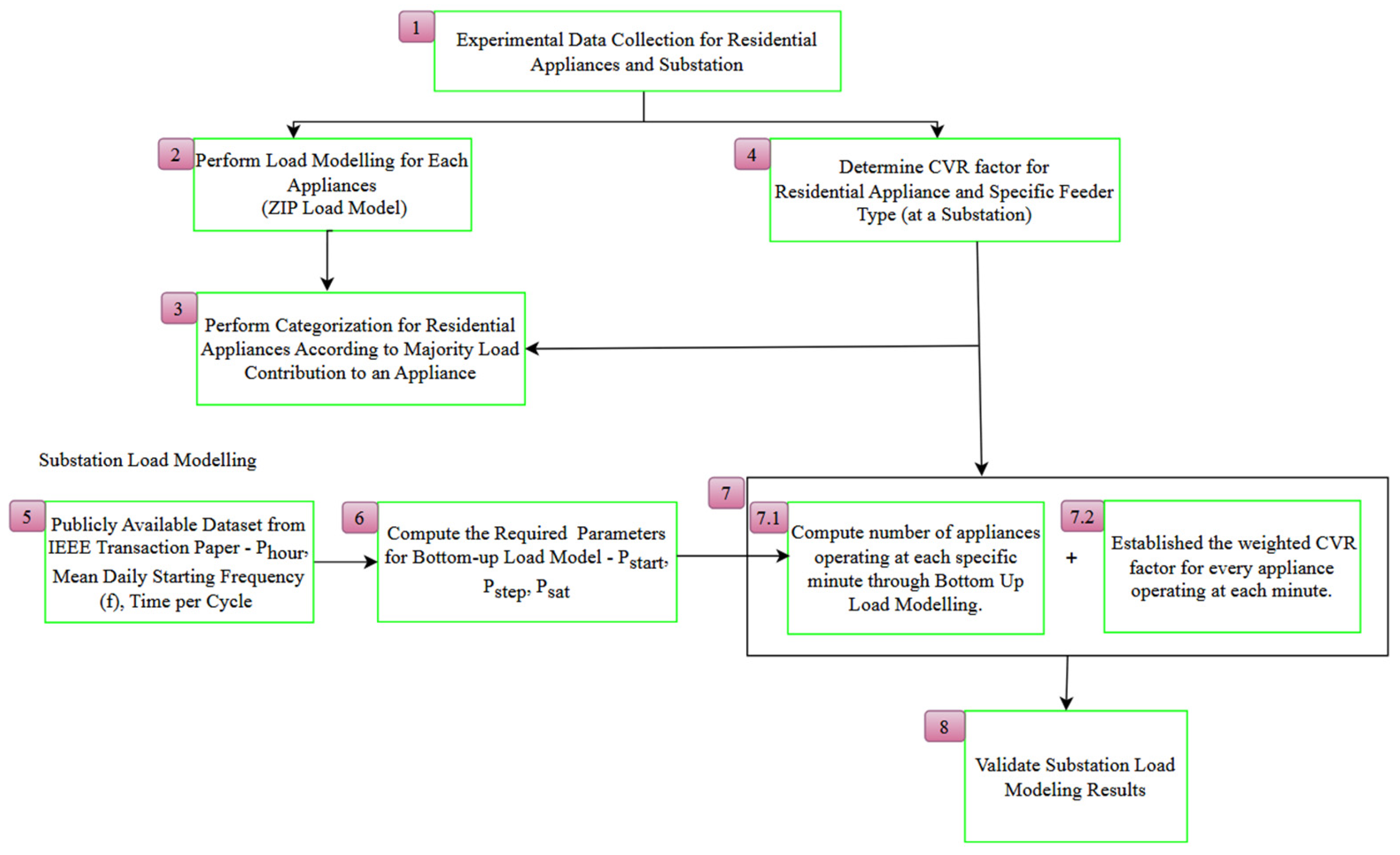
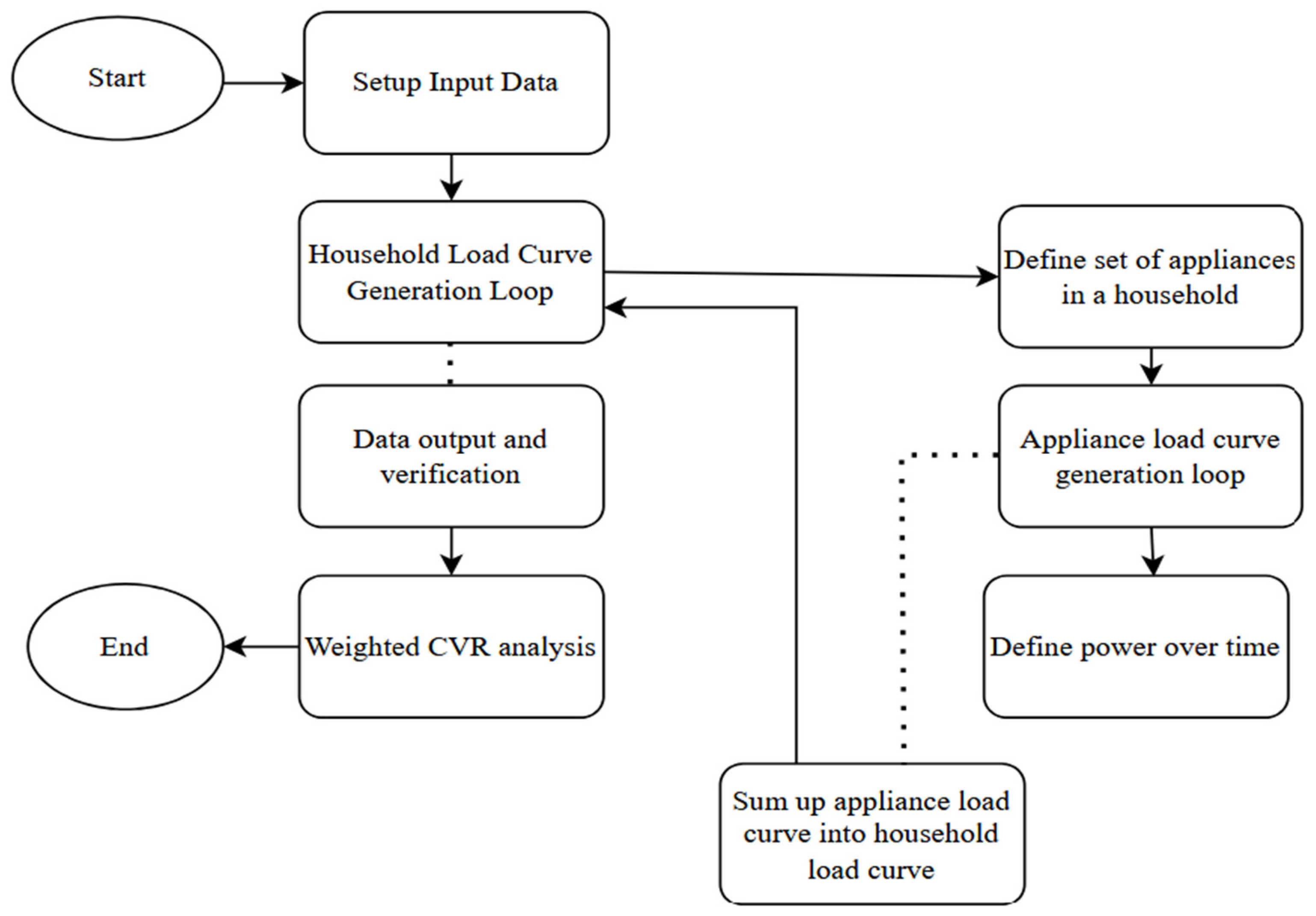
The overall methodology for this study is as displayed in Figure 1 below. The requisite data for this study’s analysis were meticulously gathered from laboratory and substation measurements. Firstly, Block 1 displays the laboratory data collection involving the measurements of 16 appliances spanning a range of voltages from 250 V to 215 V, with decremental voltage adjustments of 5 V. The corresponding power readings were logged to ascertain the ZIP load model for each appliance. The details of the appliances will be discussed in the next section. The data collection at the laboratory and substation was conducted with a 1 s per time step. These carefully collected appliances’ datasets were subsequently subjected to optimization techniques in Python (Spyder 5.5.4) to derive the ZIP load model as shown in Block 2. Then, in Block 3, the subsequent load categorization hinged upon the insights from the load model analysis results. The appliance and substation dataset collected was transformed into the CVRf for further analysis as established in Block 4. Consequently, as expressed in Block 5, a bottom-up load model study was incorporated in the pursuit of further verifying the findings of this research. The data required for the bottom-up load model were obtained through surveys which are available in the IEEE Transaction paper that was published for Singapore [29]. In Block 6, the data were used to calculate the Pstart, Pstep, and Psat values that were suitable for this study. These values were then incorporated into a Python script to be compared with random numbers generated by the software. If the random number generated was smaller than the Pstart, then the appliance would turn “on”. The turn on duration contributes to the power accumulated for every minute as shown in Block 7.1. The analysis and graphs generated are for 1440 min and a day. They were used to observe the power consumption and the appliance behavior in a day. In Block 7.2, a weighted CVRf was generated from the bottom-up load model for 120 houses (based on each appliance usage) corresponding to the CVRf for a residential substation. In this analysis, the measured substation CVRf was validated with the simulated bottom-up load modeling CVRf as exhibited in Block 8. The focus of this paper will be on active power data, as these are the greatest determinants of residential load behavior, billing, and energy consumption in Malaysia.

Figure 1.
Overall flowchart.
3.2. Data Collection/Experimental Scenario
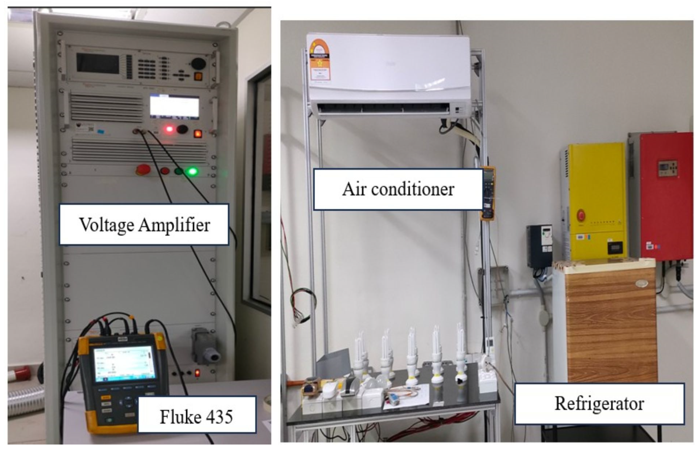
This paper focuses on the Malaysian residential scenario. The appliances that were used to collect the data are basic appliances that exist in most residential households with regard to all types of residential class. The data for analysis were obtained from the measurements conducted in the laboratory. There were 16 common items of household equipment used for the ZIP and CVR measurements. The load profile was obtained by changing the input voltage from 250 V to 215 V. This range was utilized to reflect the permissible range of voltage fluctuations under the Malaysian Tenaga Nasional Berhad (TNB) standard, which allows a variation of +10% to −6% from the nominal voltage of 230 V. TNB is Malaysia’s sole power distributor and the largest electricity producer in the country. By adjusting the voltage within this range, the study captured the real-world operating conditions of appliances experienced in Malaysia. This ensured that the derived ZIP load model and CVR analysis accurately represents the appliance behavior under typical voltage deviation standards. Moreover, testing within this range allows for the assessment of how voltage variations impact power consumption, load dynamics, and overall power quality, aligning the study with practical and regulatory considerations. The voltage supply was adjusted in 5 V increments to align with the low-voltage transformer tap changer behavior and ensure consistency with previous research methodologies. This step size captures the detailed, incremental changes in appliance power consumption, enabling the precise derivation of ZIP load coefficients and provides a balance between resolution and practicality. The Fluke 435 Power Quality recorder was used to measure the power changes every second. The Fluke 435 Power Quality recorder was used in the analysis because it provides high-precision measurements of electrical parameters, including voltage, current, and power, with a 1 s resolution. This accuracy is crucial for capturing the subtle variations in appliance power consumption as the voltage levels change, which are essential for deriving the ZIP load model. Additionally, the Fluke 435 is specifically designed for power quality analysis, ensuring reliable data collection under diverse conditions and making it well suited for both the laboratory and substation measurements required in this study. The equipment that was tested included an air conditioner, CFL light, fluorescent light, incandescent light, LED light, fan, laptop, personal computer (PC), phone, tablet, television (TV), microwave, rice cooker, shower heater, kettle, and refrigerator. Figure 2 below shows the connection established in the laboratory for the measurement.

Figure 2.
Laboratory measurement apparatus setup.
The measurement condition with data recorded at 1 s time intervals for every appliance was a room set at an initial temperature of 27 °C, and the air conditioner (conventional 1 horsepower) was measured for a duration of 5 h. For each 5 V reduction from 250 V to 215 V, the corresponding power was directly measured in a room in the lab with no occupancy. It was also ensured that the air conditioner was not to be immediately switched on for the next measurement. It was allowed to cool down as the usage was replicated for a similar situation in a residence. The temperature of the air conditioner was set at 20 °C, the mode was set to cold, and the fan speed was set to automatic. Eight power measurements with varying voltages were recorded and analyzed for the load modeling and CVR factor calculation.
As for the refrigerator (conventional empty mini bar), the internal temperature was set as constant throughout the measurement, which was conducted for a duration of 24 h. Each time the measurement was performed, the refrigerator was defrosted and then turned on as a new refrigerator, and the corresponding voltage and power were recorded. The electric kettle (1 L capacity) is another common domestic device that is available in every household. The electric kettle was also used to measure the power at every voltage variation and the data were recorded for every cycle of 1 L of water reaching a rolling boil.
As for the other appliances, the duration of measurement was determined based on the power behavior of the appliances regarding the voltage change where every voltage reduction displayed a consistent power behavior for each voltage drop. As for the lighting devices such as the incandescent, CFL, florescent, and LED lights, each light was measured for a duration of 50 min. This similar concept was utilized for the fan (stand fan, 3 blades—speed 3), laptop while being charged, tablet, shower heater (conventional water heater—without a pump and at a medium temperature), PC, handphone (android), and TV (40-inch television). However, for the microwave (manual microwave), the measurement was conducted for a duration of 1 min for every voltage change, and as for the rice cooker (manual 1.8 L), the measurement was recorded throughout the duration of rice being cooked.
Heating and cooling [30] are the largest components of residential electricity consumption. Air conditioning is a crucial appliance for many people in Malaysia to help combat the high temperatures and humidity levels. Efficient and sustainable heating and cooling solutions, such as energy-efficient appliances, CVR, and renewable energy systems, can help to reduce the energy consumption and associated costs while maintaining a comfortable indoor environment.
Upon obtaining the individual appliances’ analysis, the substation measurement aimed to confirm the precision of the CVR models specifically tailored for individual households. The voltage reduction for a substation however was based on natural occurrences of voltage dips because the testing was performed under live conditions and manually tempering with the voltage through tap changers was not allowed as this was a feasibility study to analyze the possibility of implementing CVR at the substation level. As a result, whenever a voltage drop occurred before the tap changer was “auto-corrected”, deviations in the power readings were observed. For this reason, when there was a drop in power at the same instance at the 11 kV and 0.4 kV feeder, with a significant drop in voltage of more than 2.3 V, those data would be used to determine the CVRf of the residential substation. The data collection was performed over 3 days for 24 h with a time step of one second per feeder at the phases AN, BN, and CN. The feeder was selected based on a 100% residential load to analyze the impact of CVR on a residential distribution network.
3.3. ZIP Load Model Analysis
This study implemented the measurement-based model which is a common load modeling technique which gathers load data from data acquisition equipment to deduce its load characteristics. Equation (1) shows that Zp, Ip, and Pp are the model parameters which represent the percentages of constant impedance, constant current, and constant power load in an appliance [31]. The parameter representation for the equations is explained below.
Equation (2) shows the constraints of the load types being totaled as 100% which is equal to 1. All loads have some variability based on the composition of constant impedance (Z), constant current (I), and constant power (P) percentages. In this study the ZIP load model shows the voltage dependency of each load and is solved using the Sequential Least Squares Programming optimizer (SLSQP) on Python using Equations (1) and (4). SLSQP was used to determine the ZIP coefficients because it is a powerful optimization algorithm suitable for solving constrained nonlinear problems, such as fitting the ZIP model coefficients to the measured power data. The ZIP load model requires accurately estimating parameters (constant impedance, constant current, and constant power components) that minimize the error between the measured and modeled power under varying voltage levels. SLSQP handles the nonlinearities of the ZIP model effectively while incorporating constraints, such as coefficients which sum to 1 and non-negative values. Its ability to perform optimization with bounds and constraints makes it ideal for this complex parameter estimation. The optimization is achieved by determining the minimum MAE value using Equation (3) and MAPE using Equation (4) by comparing the calculated PZIP and measured PZIP values. The best fit line that provides the smallest error value stipulates the most suitable ZIP percentage representation for each appliance. Most researchers introduce one constraint for the ZIP analysis, which is that the total ZIP load coefficients must sum to 1; however, an additional constraint was introduced in this study which was to only allow positive values for the ZIP load coefficients which were between 0 and 1. This approach was chosen as it more accurately reflects the appliance usage in a Malaysian residential scenario. This is because only the power consumed by the appliances is considered in the energy calculation, while negative load contributions, which represent power feedback into the grid, are excluded from this analysis.
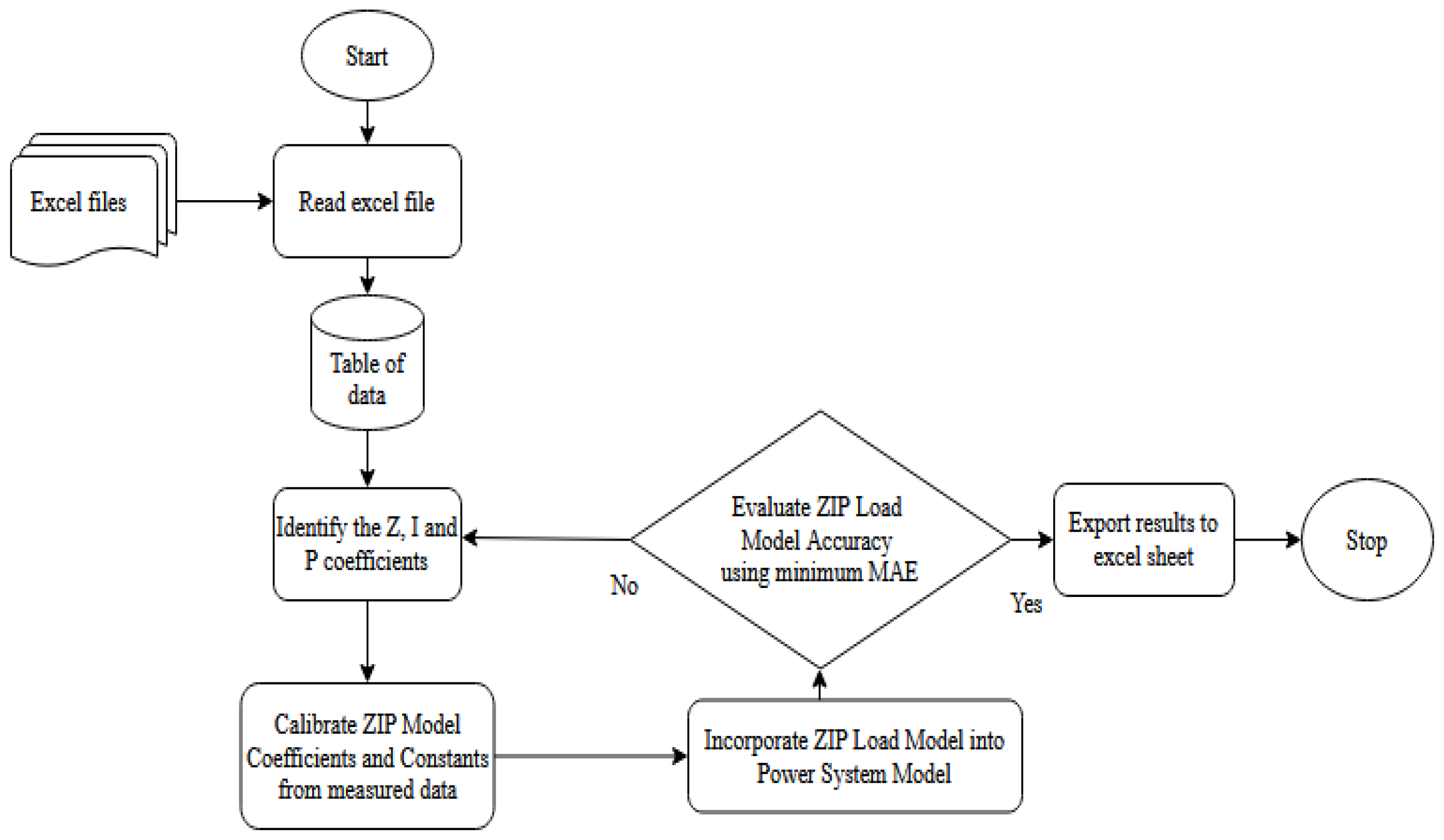
Based on the equations displayed above, P0 refers to the initial steady-state active power, V0 refers to the initial steady state-voltage, V refers to the new voltage, the ZP, IP, and PP represent the impedance and current terms that act like sensitives around the base constant powers [32], and n refers to the number of appliances used in this study. Figure 3 shows the flow chart used to determine the ZIP load model where the data collected from Section 3.2 were incorporated into the Python script to identify the ZIP coefficients and confirm that the values comply with the constraints of summing to 100% and that the ZIP values must be positive. The initial ZP, IP, and PP values are estimated small numbers, and multiple iterations were performed to determine the most suitable ZIP value. The PZIP measured and calculated was used to determine the MAE error value by incorporating the ZIP load values into the power system model represented by PZIP. Thereafter, the smallest MAE value shall represent the ZIP load model for each specific appliance.
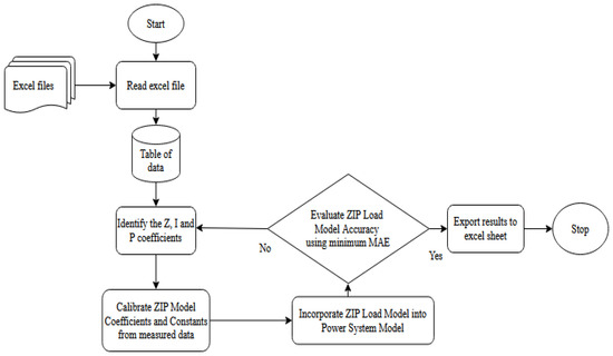
Figure 3.
Flow chart of ZIP load model.
3.4. CVR Analysis
Voltages at consumer premises should be kept at 1 (pu) volts within the range of −6% to +10% from the base voltage [33]. For the measurement and verification of CVR, there are four methods that can be used which include: comparison, regression-based, synthesis, and simulation-based methods, which are explained in detailed in [34]. The method used to resolve the CVR analysis in this research was by implementing the synthesis-based method for the residential appliances as the devices were measured with precision in the laboratory.
Equations (5) and (7) were used to compute the CVRf for this analysis. Vafter means the voltage level after the change in voltage, and Vpre is the voltage before, while Vmean is the average of the two values as displayed in Equation (5). A similar formula was used to calculate the percentage change in power (ΔP%) with the respective values measured at the same instance that the voltage drop takes place. The CVRf values were calculated using Equation (6). In Equation (6), % ΔP is the percentage reduction in the total active power consumed by the network, whereas % ΔV is the percentage reduction in the supply voltage, and for this study, it represents the percentage reduction in voltage supplied to the loads. Eight values of CVRf that were calculated for each voltage drop for every device were averaged to determine the CVRf of each appliance as presented in Equation (7).
The characteristics of residential appliances’ CVRf are divided into elements such as constant impedance, constant current, and constant power, summarizing the CVRf values responding to the voltage reduction. This specific range of numbers are referenced in [35], as the basis for appliance categorization corresponding to the CVRf values generated. These values were cross-referenced with the ZIP load model calculation to identify the appropriate load classification, which will be discussed in Section 4.
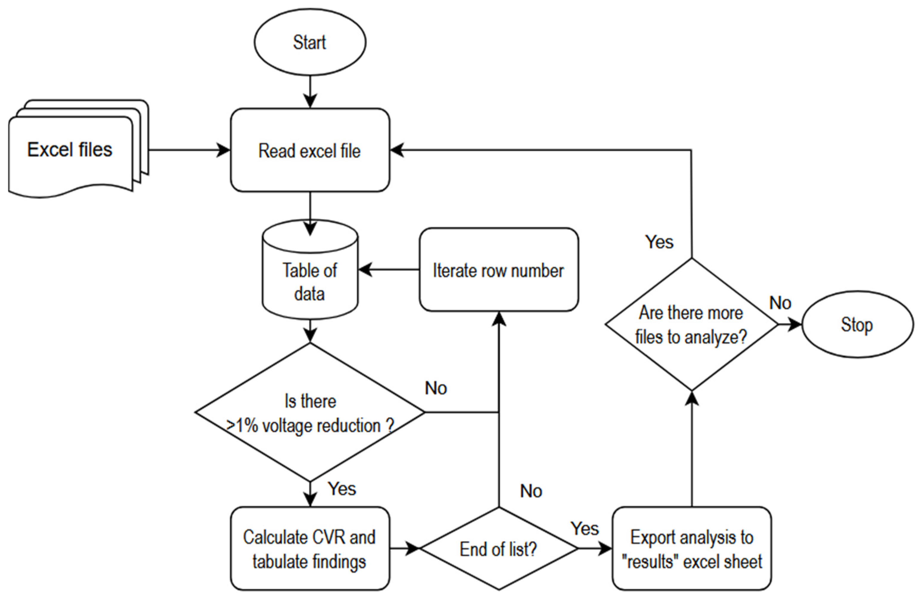
Figure 4 illustrates the flowchart used to determine the CVRf for the substation network. A Python script extracts values from the data, which are then used to calculate the CVRf for the system each day. Every data point is compared with subsequent values, and a voltage drop exceeding 2.3 V triggers the CVRf calculation. The analysis of residential appliances’ CVR was verified by comparing it with the daily 100% residential substation CVRf.
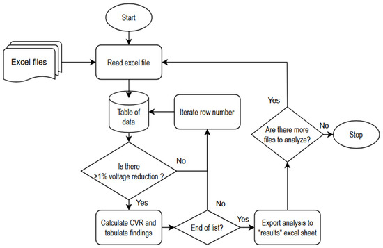
Figure 4.
Flowchart to determine the substation CVRf.
3.5. Bottom-Up Load Model Analysis
The bottom-up load model simulates a household’s total power consumption by considering the statistical usage patterns of each individual appliance. This approach constructs the overall load by combining the fundamental components, such as individual appliances or homes, to provide a precise representation of the total load at the substation level. One of the key strengths of this approach is its ability to evaluate the specific impact of each appliance on the total power consumption.
This approach can be scaled to a residential feeder containing 120 homes by aggregating the individual household data to generate a comprehensive load profile. Each home’s appliance usage patterns are modeled to capture the unique energy consumption behaviors. This study replicated the method and data from [29] with some modifications, such as using Python as the software for the analysis and incorporating the CVR analysis performed in this study. In the bottom-up approach, individual household appliances are modeled to estimate the overall load, with the calculation incorporating Equation (8), where Pstart represents the starting probability. Factors like Phour, the hourly load profile, and Pstep, the scaling factor for the step size, are also included in the formula. The saturation probability, Psat, was set to 1, to reflect the appliance availability at every residence.
Additionally, the CVRf calculated in this study was integrated into the bottom-up model analysis to generate the CVRf both at the household level and for the entire residential substation. The simulation process for the bottom-up load model is depicted in the flowchart in Figure 5, providing a clear overview of the steps used in the analysis. This structured approach ensures consistency and accuracy throughout the modeling process.
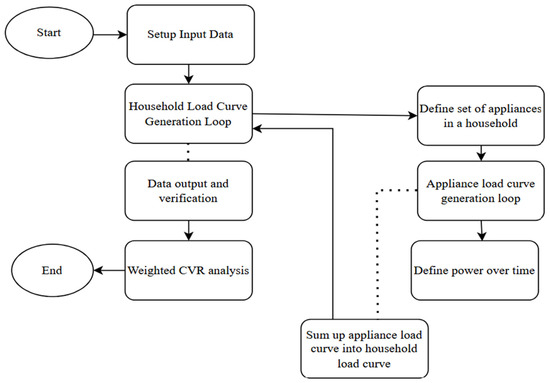
Figure 5.
Bottom-up load model energy analysis flow chart.
This research adapted the method and data from [29] but by making the necessary alterations, such as using Python as the software used, and the Psat was equal to 1 with the Pstart recalculated to suit this analysis, which is explained in detail below. As such, the data collected in Singapore were used instead—as the input for this modeling, mainly due to the following considerations:
- i.
- Both Singapore and Malaysia share similar physical and meteorological characteristics, as well as a tropical climate and comparable ethnic communities and demographic structures.
- ii.
- In Singapore and Malaysia, household electrical appliance models and power usage are similar.
- iii.
- Malaysia has a similar grid utility infrastructure, the same voltage level and uses the same type of sockets: both are 400/230 V for household electricity.
- iv.
- Both Singapore and Malaysia are in the same time zone and adjacent to each other.
The probability of start (Pstart), calculated using Equation (9), was recalculated for each device to suit the specific conditions of this study. This recalculation was based on the probability of saturation (Psat) and the step size scaling factor (Pstep) suitable for this analysis. These probabilities, Pstart, Psat, and Pstep, are crucial for the analysis because they directly influence the accuracy and reliability of the simulated load profiles for residential buildings. Pstart determines the likelihood of an appliance being activated at any given time, which is essential for modeling realistic usage patterns. Psat reflects the availability of appliances within a household, ensuring that the model accounts for the actual number of appliances, thereby affecting the total load calculation. Pstep allows for the scaling of probabilities according to the time step of the simulation, which is important for capturing the temporal dynamics of energy consumption accurately. Together, these probabilities enable the model to simulate the household electricity consumption behavior more effectively. For this study, Psat was set to 1 based on the availability of appliances in a residence, and Pstep was calculated using Equation (9). The Pstep parameter reflects the average daily startup frequency of a given appliance, which is averaged per hour by dividing the total number of startups by 24 (the number of hours in a day). This gives the average number of appliance startups per hour. Once an appliance starts, it runs for a fixed period of time, referred to as Tcycle. During this cycle, no further checks for starting are required, as Tcycle minus one indicates that no additional startup choices are made during this time. The mean daily starting frequency (f) models how often an appliance is used on average each day, while the hourly probability factor (Phour) represents the probability of usage at specific times of the day.
Pstart = Phour × f × Pstep × Psat
To simulate this, a random number generator in Python was used to compare the values. An appliance is turned “on” when the starting probability Pstart exceeds a randomly generated number between 0 and 1. After the appliance turns off, the starting probability is re-evaluated using Pstart. If the appliance starts again, its nominal power consumption (Pnom) is added to the household’s total load curve (Ptot). For appliances with standby power consumption (Pstandby), this standby power is included in the total load curve at all times, regardless of whether the appliance is actively in use or idle, as outlined in Equation (10). Additionally, a plot was generated for the weighted average CVRf (WCVR) based on Equation (11), which calculates the CVRf for each minute according to the contribution of appliances that are turned on at that time. Equation (11) is summed for each household and divided by the total number of houses analyzed to determine the weighted CVRf per minute, representing the CVRf of a residential feeder. This was performed for the number of appliances (n) analyzed in this study.
The purpose of validating the measured substation CVRf against the bottom-up load-model-simulated CVRf is to ensure that the model accurately represents the real-world response of the substation to voltage changes and vice versa. This validation helps confirm that the model can reliably predict how a load will respond to voltage adjustments, supporting its use in grid planning, operational decision making, and voltage control strategies. By comparing the measured and simulated CVRf, utilities can assess the model’s accuracy, identify discrepancies, and enhance the confidence in its application for system stability and energy efficiency.
This approach was best suited for the study since it incorporates intricate, multi-level data collection and modelling strategies to guarantee precision and usefulness. By combining controlled laboratory measurements with real-world substation data, it captures precise appliance behaviours and broader system dynamics. The use of ZIP load modelling and Python-based optimization provides a robust framework for understanding voltage-dependent appliance responses. Additionally, the incorporation of a bottom-up modelling approach, validated through survey data and IEEE studies, ensures scalability and reliability. The validation procedure of the approach, which compares simulated and measured CVRf values, further strengthens its credibility, and the daily power usage simulations provide useful information for household energy planning and control.
4. Results and Discussion
4.1. Measurement Results
The measurement results are very essential in this research as the measured data would imply the direct correlation between the voltage and power behavior of an appliance. A voltage reduction that leads to a power reduction can be identified as the constant current or constant impedance type of loads. These devices will be very useful for energy savings. These raw data were fed into the Python programming to obtain the outputs of the ZIP model. Figure 6 displays the graphical representation of the recorded power data for various residential appliances with the voltage fluctuation measured at every 1 s time step. The data obtained illustrate how different household devices respond to a controlled voltage reduction from 250 V to 215 V, in 5 V steps reduction.
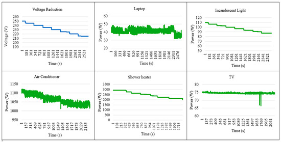
Figure 6.
Sample of recorded data for residential appliances.
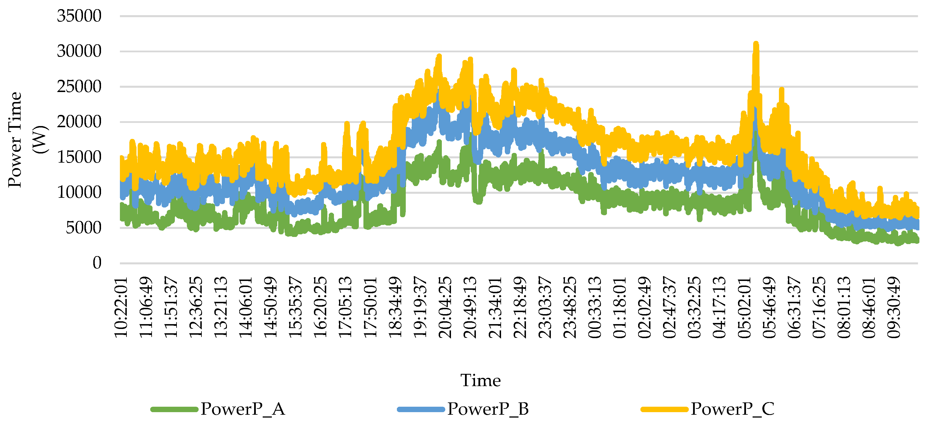
Figure 7 displays the residential substation data measured over 24 h for each phase, collected at the same substation over three days with recordings taken every second. The power pattern shows peak consumption in the morning and late evening. The CVRf was calculated only for consistent voltage drops across all three phases at the same time. This approach ensures the accuracy and reliability in determining the CVRf.
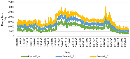
Figure 7.
Sample recorded data at the residential substation.
4.2. ZIP Load Model
A ZIP coefficient provides an understanding of the behavior of a load under different operating conditions and is a critical metric for understanding how a residential appliance responds to changes in the electrical grid. Table 1 below exhibits the values of the ZIP load model for every appliance that was measured together with the MAE and MAPE values. The ZIP load model values represent the characterization of each appliance, and these values are further compared to the calculated CVRf that will be discussed in the next section. The characterization of the appliances is crucial as it determines the response of each appliance to the voltage reduction. The MAPE provides a more meaningful indicator of the model’s accuracy in this context, as it normalizes the error relative to the actual values. Since the MAPE is within 10%, the model is acceptable, as it indicates that the percentage deviation from the true power consumption is within a tolerable range for practical applications. Thus, while the MAE might be large due to high power usage, keeping the MAPE under 10% ensures that the model remains reliable and accurate for power system analysis and energy efficiency applications. Furthermore, it has been proven in numerous publications [1] that the percentage of errors could be higher if the data that are dealt with have large values.

Table 1.
ZIP load model representation.
Based on Table 1 displayed below, it could be observed that each appliance has its own composition of constant impedance, constant current, and constant power types of loads that determines the behavior of an appliance. Appliances with high Z values, like fans and rice cookers, are highly sensitive to voltage changes, as their power consumption varies with the square of the voltage, making them suitable for energy savings in systems with voltage reduction. I-dominant devices, such as phones and CFLs, maintain a steady current and are energy-efficient under voltage variations. Meanwhile, P-dominant appliances, like refrigerators and PCs, draw consistent power due to their internal regulation mechanisms, ensuring reliable performance but potentially limiting energy savings opportunities. These differences highlight how the suitability of devices for energy savings depends on their dominant ZIP behavior and the stability of the voltage supply.
4.3. CVR Factor
The CVRf values for all 16 items of equipment that were measured and calculated are displayed in Table 2 below. The constant resistance loads generate the highest CVRf followed by a constant current load and constant power load with a lower CVRf. This finding can assist in estimating the benefits of voltage reduction for most household appliances. The calculated values of CVRf are displayed below in Table 2 with an average of total CVRf computed as 1.112. The CVRf data reveal significant variations in energy efficiency and conversion performance across the appliances. Shower heaters and fluorescent lights lead with high CVR values, indicating the optimal energy-to-output ratios. Conversely, TV and tablets show minimal efficiency, with CVR values as low as 0.058.
Table 2.
CVRf for residential load.
Different lighting technologies exhibit distinct electrical and control characteristics, causing them to respond differently to voltage changes and thus yield varying CVRf values. Incandescent lamps, being primarily resistive loads, exhibit a moderate CVRf of 1.526 because their power consumption changes roughly in proportion to the voltage. LEDs, on the other hand, maintain a relatively constant power leading to a low CVRf of 0.313. CFLs incorporate devices that regulate the current and provide a suitable starting voltage that results in a moderate CVRf of 1.308. Meanwhile, fluorescent lamps use a simpler form of current regulation, making them highly sensitive to voltage changes and producing the highest CVRf of 2.189. Even small voltage variations significantly affect the power drawn. However, TVs and tablets typically incorporate power electronics and voltage regulators designed to maintain relatively constant power consumption despite changes in the input voltage. As a result, their power usage does not vary significantly with the supply voltage, leading to low CVRf values. Addressing such inefficiencies is critical for reducing energy waste, especially in households with multiple electronic devices, making it an important factor in sustainability initiatives.
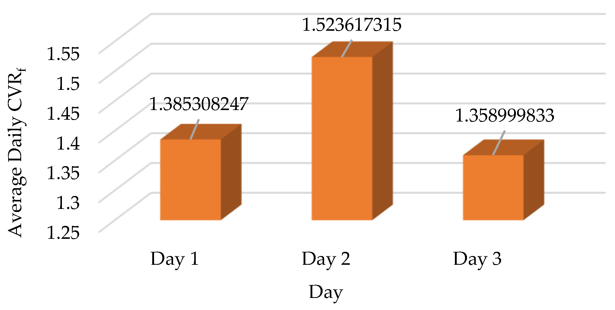
The Pencawang Pembahagian Utama (PPU) data are not displayed in this study because the PPU is connected to multiple feeders, and the medium voltage substation data are beyond the scope of this research. Instead, the focus is on the CVRf results for a low voltage residential substation, as shown in Figure 8. The CVRf results for individual loads are consistent with those for a 100% residential feeder substation. For residential appliances, the CVRf is calculated as 1.112, while the CVRf for a residential feeder varies from 1.35 to 1.52 as displayed in Figure 8. A CVRf of more than 1 supports the effectiveness of the CVR implementation, as it demonstrates a greater capacity for voltage reduction and energy savings across the entire feeder. Therefore, a voltage reduction implemented during these peak hours would result in the most significant reduction in the peak demand and offer substantial energy savings, making it ideal for planned CVR implementation.

Figure 8.
Average measured CVRf of a 100% residential substation.
Various studies have reported a wide range of residential CVRf values, highlighting the variability in voltage reduction impacts across different regions and systems. For instance, CPUC found a CVRf of 1.14 [34], while SCE reported 1.30 [19]. Snohomish’s measurements ranged from 0.33 to 0.68 [34], and HQ’s findings fell between 0.06 and 0.67 [36]. Meanwhile, NEEA documented a CVRf of 0.63 [37], and Detroit reported values from 0.96 to 1.11 [34]. It can be observed that Snohomish and HQ have a slightly lower residential CVRf value because the type of loads connected to the feeder is not a 100% residential load but a mixed load with varying percentages of residential and commercial load contributions as mentioned in the paper (unlike that used in this study—100% residential).
The main aim of this paper is to highlight the load composition of a residential appliance by performing ZIP and CVR analysis. The results obtained are then used to determine the load categorization for each appliance. The load composition of residential appliances is crucial for several reasons, primarily in the context of electrical power distribution and energy management. It aids in load profiling, enabling utilities to understand the electricity consumption patterns of different appliances and plan accordingly. This information is vital for load forecasting, helping utilities anticipate and meet future demand. The residence CVRf is established and verified with a residential substation, and the CVRf is further validated via a bottom-up load model simulation.
4.4. Load Categorization
The CVRf values are used as a reference to study the behavior of each appliance in relation to voltage reduction, and the ZIP load model finding corresponds to the CVRf determined as displayed in Table 3. The CVRf obtained through the experiments as displayed in Table 2 determines the load type shown in Table 3. It is important to note that the CVRf values from [35] are referred to for the categorization based on their respective ranges for constant impedance, constant current, and constant power elements based on the CVRf of each appliance. Constant resistance yields a CVRf of 2.0 or higher; for constant current, it falls between 1.0 and 1.99; and for constant power, it is below 1.0. Since CVRf values do not always produce neat, round numbers, this range provides a clearer way to classify the data. Numerous studies have been conducted by various countries to determine the ZIP values for each appliance. It can be observed that unlike the constraint introduced in this study, where the load composition must be a positive value, other studies indicate the ZIP load contribution in regard to negative coefficients as well. However, it is impossible to obtain identical values for similar appliances, but a common type of representation can be determined by comparing the ZIP load values from various studies. The appliance categorization is presented in this study by first obtaining the ZIP values and then the CVRf. An appliance is predominantly characterized by the load type ZP, IP, or PP that contributes the highest percentage. However, if multiple load types contribute to an appliance with less than a 30% difference between them, the appliance is classified as being influenced by two or more load types.
Table 3.
Categorization of various residential appliances based on ZIP values and CVRf.
The ZIP load categorization determined from this study and various other publication is as displayed in Table 4. The results obtained are compatible with several studies that have been conducted. Table 4 below shows the categorization performed for various ZIP load results that have been obtained over the years in various countries in addition to the results obtained in this study. Load categorization is the basic information about an appliance to determine its behavior in response to a change in voltage as it is significant to aid in energy efficiency, preventive maintenance, and optimal performance, ensuring cost savings and sustainable resource utilization in a residence.
Table 4.
Categorization of residential appliances based on various published ZIP values.
Based on the categorization performed in Table 4, the results were further enhanced by performing percentage normalization, to provide a clearer representation of the data distributions as displayed in Figure 9. The analysis of 16 appliances reveals varied load behaviors, highlighting the key trends in their categorization. The TV and PC (80% indicates constant power), refrigerators (60% indicates constant power), laptop charging and LEDs (66.7% indicates constant power) and tablet (100% indicates constant power) predominantly maintained fixed power consumption, while CFL (87.5% indicates constant current) and phones (100% indicates constant current) exhibited consistent current draws. Resistive behavior dominates in appliances such as microwaves (60% indicates constant impedance), for fans and florescent lights (66.7% indicates constant impedance) meanwhile kettle, rice cookers, and shower heaters (100% indicates constant impedance). Mixed behaviors appear in incandescent lights (85.7% indicates constant current and constant impedance) and air conditioner (a total of 50% indicates constant impedance, constant current and constant power load combination). The reliability of these results is higher for appliances with dominant percentage categories. However, appliances with distributed percentages, especially for air conditioner, microwaves and refrigerators, may reflect variations due to appliance design, operating conditions, or differences in the measurement methodologies.
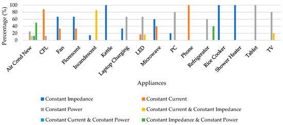
Figure 9.
Percentage normalization determined based on the ZIP load model categorization from various published data.
4.5. Bottom-Up Load Model
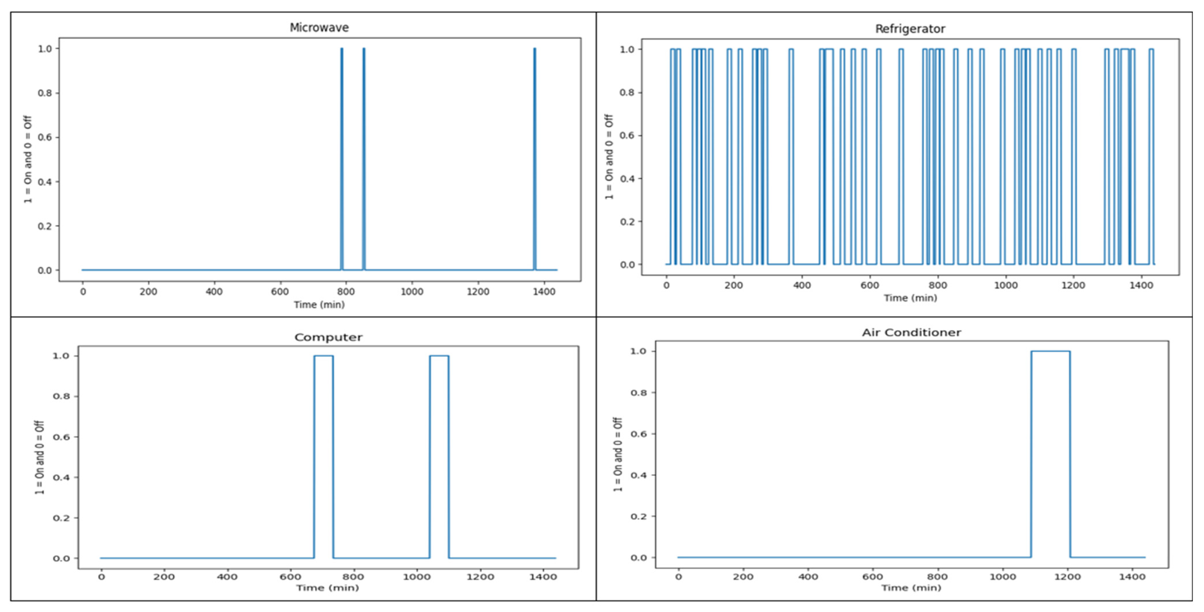
As mentioned above, understanding the load profile and behavior of appliances is essential for accurately modelling the total power consumption within a residential network. The diagrams below illustrate the activity patterns of each appliance, which are crucial for calculating the total power values. These values are derived from the duration during which each appliance is switched “on” or “off”. Figure 10 displays the daily switch-on (which is indicated with 1) and switch-off (which is indicated with 0) activities for some appliances within a household, offering a detailed view of their operation patterns. These appliance activity data must be established foremost to accurately perform the power analysis that follows, as they form the basis for the subsequent load and CVRf calculations. Without this step, the analysis of power consumption and voltage reduction effects would lack precision, underscoring the importance of understanding appliance behavior in the overall CVR strategy. The purpose of the bottom-up load model is to ensure the accuracy of the simulated CVRf in Section 4.3 above.
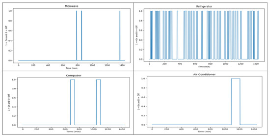
Figure 10.
Microwave, oven, computer, and refrigerator turned on/off.
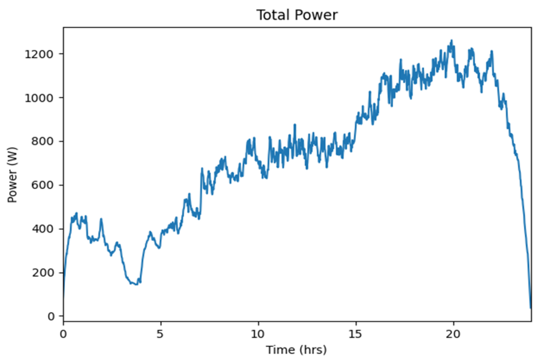
Figure 11 below shows the power consumed by one house in a day, and a similarity can be observed to the Malaysian residential power consumption pattern with higher power utilized in the morning and late evening.
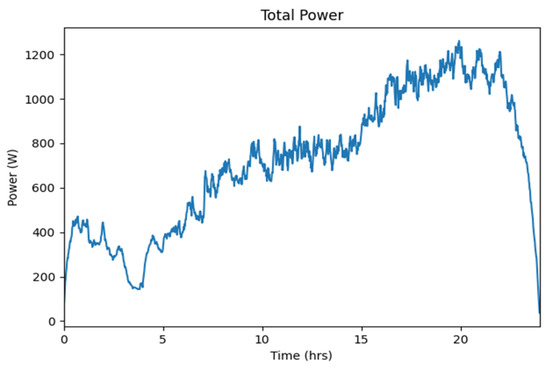
Figure 11.
Total power consumption throughout a specific day for a house.
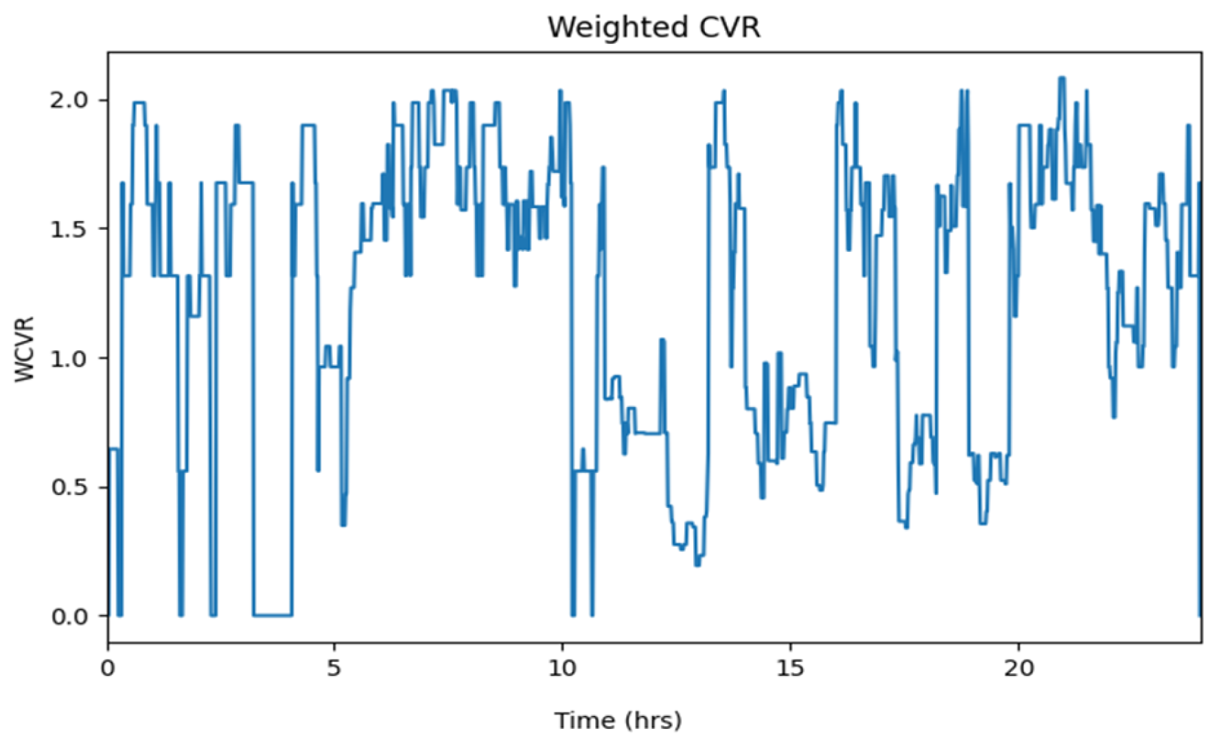
Figure 12 below indicates the weighted CVRf calculated based on the power contributed by the appliances that are switched “on” at every minute of the day. The weighted CVRf averages at 1.22 throughout the day. This value corresponds to the CVRf that is generated for a residence which is 1.112, averaged from the individual appliances CVRf measured in the laboratory.
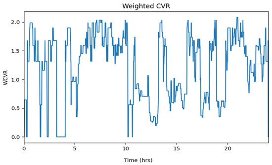
Figure 12.
Weighted CVRf per house.
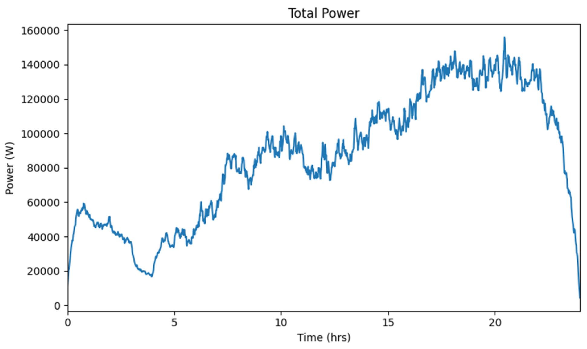
This model was also used to generate the total power consumed by 120 houses as shown in Figure 13. The power consumption of a residence pattern can be observed with higher loading values in the morning and evening. A number, 120, is used to represent the number of houses connected to a residential feeder in a Malaysian scenario.
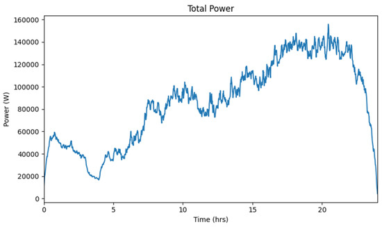
Figure 13.
Total power consumption of 120 houses in a day.
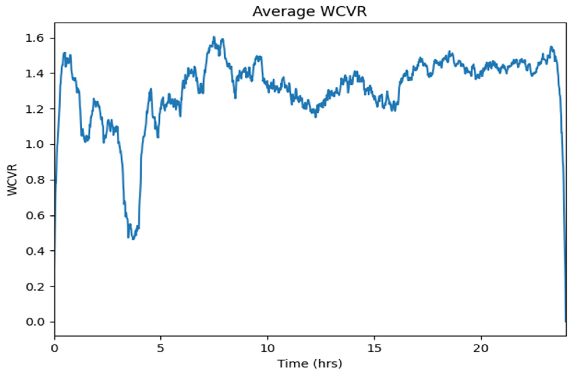
The weighted CVRf for multiple residences is validated, indicating that the results have been checked against the expected outcomes for consistency and accuracy between the measured and simulated results. The average CVRf of 1.32 was calculated for 120 houses, as illustrated in Figure 14, which falls within an acceptable range for residential applications. This value suggests that for each unit of voltage reduction, there is a corresponding reduction in energy consumption, which is a crucial aspect of effective energy management in residential settings. In contrast, the residential feeder CVRf measured at the substation are 1.385 and 1.358, respectively. The compatibility of these values indicates that the residential CVRf derived from the individual households is aligned with the aggregate performance observed at the substation level.
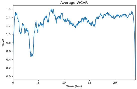
Figure 14.
Averaged weighted CVRf 120 houses.
Given this similarity, further correlation analysis is necessary to assess the consistency of the simulation in replicating real-world conditions. The comparison between the simulated and measured CVRf values reveals a close alignment at certain specific times of the day as displayed in Figure 15. Particularly in the morning at 8:51, the difference is minimal at 0.30%. The simulated and measured values show a larger discrepancy in the morning at 9:41, where the measured CVRf is 1.26930 compared to the simulated 1.35851, resulting in a 6.57% difference. Similarly, at night at 9:33, the measured CVRf is 1.44870, showing a 4.00% deviation from the simulated 1.50899. Despite these differences, the overall trends are similar, indicating a strong relationship between the simulated and measured data.
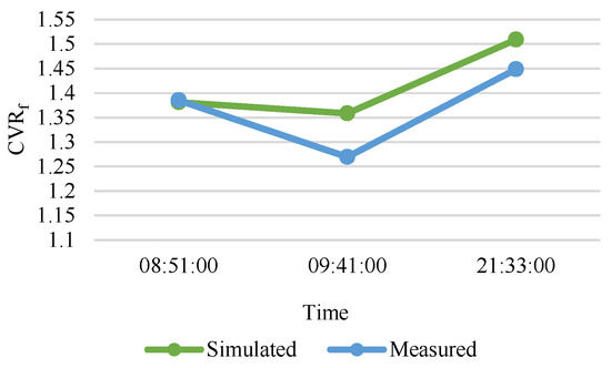
Figure 15.
Simulated vs measured CVRf comparison at specific time in a day.
This validation confirmed that the simulated CVRf closely aligns with the measured CVRf from the residential substation, demonstrating the model’s accuracy and reliability for predicting the load response to voltage changes. A CVRf exceeding 1 is indicative of significant potential for peak shaving and energy savings within residential networks. Specifically, it means that as the voltage is reduced, the corresponding energy consumption declines, which can help utilities manage peak demand more effectively. The alignment of these factors suggests that bottom-up load modeling effectively captures the dynamic behavior of residential loads and their response to voltage changes. Nevertheless, when comparing simulated to measured CVRf results, discrepancies often arise because simulations tend to be idealized and operate strictly within their programmed parameters. Even when data are randomized, the model may not fully capture the dynamic behaviors or sudden load changes that occur in an actual substation. Real-world loads, by contrast, represent a constantly shifting mix of end-use equipment, each with its own time-varying voltage dependencies.
5. Conclusions
The recorded voltage and power data were used to derive the ZIP load model and also CVRf of residential appliances. The load model for various residential appliances and a categorization were successfully performed to further establish the results of this research. The CVRf values for 16 different items of house equipment were determined, and the types of loads were also categorized accordingly, complementing the ZIP load model categorization. The percentage normalization expresses reliable data for 13 appliances with dominant percentages, while 3 (air conditioner, microwave and refrigerator) have mixed distributions.
Constant resistance and constant current loads yield a higher CVRf. The results show that 50% of the measured residential appliances consist of a combination of constant impedance and constant current loads, making CVR both suitable and effective for these types of loads. The CVRf findings indicate that the CVRf of a house is 1.112, the averaged measured residential feeder CVRf is between 1.358 and 1.52, and the averaged simulated residential feeder CVRf is 1.32. The measured and simulated CVRf at specific times of the day also demonstrate consistent results with good correlation, showing a deviation of less than 7%.
By simulating the residential power consumption through the aggregation of individual appliance usage data and the incorporation of human behavior, a bottom-up load model coupled with CVRf analysis offers deeper insights into how voltage reductions affect the different households connected to a substation. This paper developed a load model and CVRf to achieve appliance categorization for Malaysian residences, which is crucial for aiding energy efficiency and cost-saving decisions.
Author Contributions
Conceptualization, M.S.B.S. and C.T.; data curation, M.S.B.S.; formal analysis, M.S.B.S.; investigation, M.S.B.S.; methodology, M.S.B.S.; project administration, J.S., A.H.A.B., and C.T.; resources, M.S.B.S.; software, M.S.B.S. and W.T.C.; supervision, J.S., A.H.A.B., and C.T.; validation, M.S.B.S. and C.T.; writing—original draft, M.S.B.S.; writing—review and editing, M.S.B.S. All authors have read and agreed to the published version of the manuscript.
Funding
This research received no external funding.
Data Availability Statement
The dataset used and/or analyzed during the current study is available from the corresponding authors on reasonable request because the data is utilized for current ongoing study.
Conflicts of Interest
The authors declare no conflicts of interest.
References
- Bircan, M.; Durusu, A.; Kekezoglu, B.; Elma, O.; Selamogullari, U.S. Determination of zip coefficients for residential loads. Pressacademia 2017, 5, 176–180. [Google Scholar] [CrossRef]
- Seva, M.; Abdullah, K.; Busrah, I.A.M.; Zin, N.D.R.M.; Balasubramaniam, I.Y.; Daud, M.H.M.; Pauzai, N.S.B. Analysis of Conservation Voltage Reduction (Cvr) Factor for Various Types of Loads. Int. J. Eng. Appl. Sci. Technol. 2020, 5, 66–72. [Google Scholar] [CrossRef]
- Yadav, G.; Liao, Y.; Jewell, N.; Ionel, D.M. CVR Study and Active Power Loss Estimation Based on Analytical and ANN Method. Energies 2022, 15, 4689. [Google Scholar] [CrossRef]
- Ma, Z.; Xiang, Y.; Wang, Z. Robust Conservation Voltage Reduction Evaluation Using Soft Constrained Gradient Analysis. IEEE Trans. Power Syst. 2022, 37, 4485–4496. [Google Scholar] [CrossRef]
- Bircan, M.; Durusu, A.; Kekezoglu, B.; Elma, O.; Selamogullari, U.S. Experimental determination of ZIP coefficients for residential appliances and ZIP model based appliance identification: The case of YTU Smart Home. Electr. Power Syst. Res. 2020, 179, 106070. [Google Scholar] [CrossRef]
- Chuan, L.; Rao, D.M.K.K.V.; Ukil, A. Load profiling of Singapore buildings for peak shaving. In Proceedings of the Asia-Pacific Power and Energy Engineering Conference (APPEEC), Hong Kong, China, 7–10 December 2014. [Google Scholar] [CrossRef]
- Zhang, Q.; Guo, Y.; Wang, Z.; Bu, F. Distributed Optimal Conservation Voltage Reduction in Integrated Primary-Secondary Distribution Systems. IEEE Trans. Smart Grid 2021, 12, 3889–3900. [Google Scholar] [CrossRef]
- Ozdemir, G.; Baran, M. A new method for Volt–Var optimization with conservation voltage reduction on distribution systems. Electr. Eng. 2020, 102, 493–502. [Google Scholar] [CrossRef]
- Sundaram, M.S.B.; Tan, C.; Selvaraj, J.; Abu Bakar, A.H. Energy Savings for Various Residential Appliances and Distribution Networks in a Malaysian Scenario. Energies 2023, 13, 4902. [Google Scholar] [CrossRef]
- Stanescu, D.; Enache, F.; Popescu, F. Smart Non-Intrusive Appliance Load-Monitoring System Based on Phase Diagram Analysis. Smart Cities 2024, 7, 1936–1949. [Google Scholar] [CrossRef]
- Chabane, L.; Drid, S.; Chrifi-Alaoui, L.; Delahoche, L. Energy consumption prediction of a smart home using non-intrusive appliance load monitoring. Int. J. Syst. Assur. Eng. Manag. 2023, 15, 1231–1244. [Google Scholar] [CrossRef]
- Faustine, A.; Pereira, L. Improved appliance classification in non-intrusive load monitoring using weighted recurrence graph and convolutional neural networks. Energies 2020, 13, 3374. [Google Scholar] [CrossRef]
- Ghosh, S.; Panda, D.K.; Das, S.; Chatterjee, D. Cross-Correlation Based Classification of Electrical Appliances for Non-Intrusive Load Monitoring. In Proceedings of the 2021 International Conference on Sustainable Energy and Future Electric Transportation, SeFet 2021, Hyderabad, India, 21–23 January 2021. [Google Scholar] [CrossRef]
- Arif, A.; Wang, Z.; Wang, J.; Mather, B.; Bashualdo, H.; Zhao, D. Load Modeling—A Review. IEEE Trans. Smart Grid 2017, 9, 5986–5999. [Google Scholar] [CrossRef]
- Goldin, A.; Buechler, E.; Rajagopal, R.; Rivas-Davila, J. Time and voltage domain load models for appliance-level grid edge simulation and control. Electr. Power Syst. Res. 2021, 190, 106750. [Google Scholar] [CrossRef]
- Hasan, M.K.; Ahmed, M.M.; Wani, N.F.; Abbas, A.H.; Alkwai, L.M.; Islam, S.; Habib, A.A.; Hassan, R. Dynamic load modeling for bulk load-using synchrophasors with wide area measurement system for smart grid real-time load monitoring and optimization. Sustain. Energy Technol. Assess. 2023, 57, 103190. [Google Scholar] [CrossRef]
- Nourollahi, R.; Salyani, P.; Zare, K.; Mohammadi-Ivatloo, B.; Abdul-Malek, Z. Peak-Load Management of Distribution Network Using Conservation Voltage Reduction and Dynamic Thermal Rating. Sustainability 2022, 14, 11569. [Google Scholar] [CrossRef]
- Behzadirafi, S.; Malallah, Y.; Qaseer, L.; de León, F. Theoretical and Experimental Verification of CVR Energy Savings for Refrigeration Loads. IEEE Trans. Power Deliv. 2023, 38, 2489–2499. [Google Scholar] [CrossRef]
- Hossein, Z.S.; Khodaei, A.; Fan, W.; Hossan, S.; Zheng, H.; Fard, S.A.; Paaso, A.; Bahramirad, S. Conservation voltage reduction and Volt-VAR optimization: Measurement and verification benchmarking. IEEE Access 2020, 8, 50755–50770. [Google Scholar] [CrossRef]
- Shim, K.-S.; Go, S.-I.; Yun, S.-Y.; Choi, J.-H.; Nam-Koong, W.; Shin, C.-H.; Ahn, S.-J. Estimation of conservation voltage reduction factors using measurement data of KEPCO system. Energies 2017, 10, 2148. [Google Scholar] [CrossRef]
- Bokhari, A.; Raza, A.; Diaz-Aguilo, M.; de Leon, F.; Czarkowski, D.; Uosef, R.E.; Wang, D. Combined Effect of CVR and DG Penetration in the Voltage Profile of Low-Voltage Secondary Distribution Networks. IEEE Trans. Power Deliv. 2016, 31, 286–293. [Google Scholar] [CrossRef]
- Wang, S.; Deng, X.; Chen, H.; Shi, Q.; Xu, D. A bottom-up short-term residential load forecasting approach based on appliance characteristic analysis and multi-task learning. Electr. Power Syst. Res. 2021, 196, 107233. [Google Scholar] [CrossRef]
- Gao, B.; Liu, X.; Zhu, Z. A bottom-up model for household load profile based on the consumption behavior of residents. Energies 2018, 11, 2112. [Google Scholar] [CrossRef]
- Tsuji, K.; Sano, F.; Ueno, T.; Saeki, O. Bottom-Up Simulation Model for Estimating End-Use Energy Demand Profiles in Residential Houses Development of the Bottom-Up Simulation Model. ACEEE Summer Study Energy Effic. Build. 2004, 2, 342–355. [Google Scholar]
- Bugaje, B.; Rutherford, P.; Clifford, M. A systems dynamics approach to the bottom-up simulation of residential appliance load. Energy Build. 2021, 247, 111164. [Google Scholar] [CrossRef]
- Parker, A.; Alkrch, M.A.; James, K.; Almaghrebi, A.; Alahmad, M.A. Framework to Develop Time- and Voltage-Dependent Building Load Profiles Using Polynomial Load Models. IEEE Access 2021, 9, 128328–128344. [Google Scholar] [CrossRef]
- El-Shahat, A.; Haddad, R.J.; Alba-Flores, R.; Rios, F.; Helton, Z. Conservation voltage reduction case study. IEEE Access 2020, 8, 55383–55397. [Google Scholar] [CrossRef]
- Jierula, A.; Wang, S.; Oh, T.-M.; Wang, P. Study on accuracy metrics for evaluating the predictions of damage locations in deep piles using artificial neural networks with acoustic emission data. Appl. Sci. 2021, 11, 2314. [Google Scholar] [CrossRef]
- Chuan, L.; Ukil, A. Modeling and Validation of Electrical Load Profiling in Residential Buildings in Singapore. IEEE Trans. Power Syst. 2015, 30, 2800–2809. [Google Scholar] [CrossRef]
- Shen, Y. Assessment of Conservation Voltage Reduction on HV and LV Distribution Networks. Ph.D. Thesis, The University of Manchester, Manchester, UK, 2018. [Google Scholar]
- Bokhari, A.; Alkan, A.; Dogan, R.; Diaz-Aguilo, M.; De Leon, F.; Czarkowski, D.; Zabar, Z.; Birenbaum, L.; Noel, A.; Uosef, R.E. Experimental determination of the ZIP coefficients for modern residential, commercial, and industrial loads. IEEE Trans. Power Deliv. 2014, 29, 1372–1381. [Google Scholar] [CrossRef]
- Jereminov, M.; Hooi, B.; Pandey, A.; Song, H.-A.; Faloutsos, C.; Pileggi, L. Impact of Load Models on Power Flow Optimization. In Proceedings of the 2019 IEEE Power & Energy Society General Meeting (PESGM), Atlanta, GA, USA, 4–8 August 2019; pp. 1–5. [Google Scholar]
- Tenaga National Sustainability Report. Energy To Sustain Communities. 2018, pp. 1–108. Available online: www.tnb.com.my (accessed on 20 January 2020).
- Wang, Z.; Wang, J. Review on implementation and assessment of conservation voltage reduction. IEEE Trans. Power Syst. 2014, 29, 1306–1315. [Google Scholar] [CrossRef]
- Sen, P.K.; Lee, K.H. Conservation Voltage Reduction Technique: An Application Guideline for Smarter Grid. IEEE Trans. Ind. Appl. 2016, 52, 2122–2128. [Google Scholar] [CrossRef]
- Lefebvre, S.; Gaba, G.; Ba, A.-O.; Asber, D.; Ricard, A.; Perreault, C.; Chartrand, D. Measuring the efficiency of voltage reduction at Hydro-Québec distribution. In Proceedings of the 2008 IEEE Power and Energy Society General Meeting—Conversion and Delivery of Electrical Energy in the 21st Century, Pittsburgh, PA, USA, 20–24 July 2008; pp. 1–7. [Google Scholar] [CrossRef]
- Williams, B. Distribution capacitor automation provides integrated control of customer voltage levels and distribution reactive power flow. In Proceedings of the Power Industry Computer Applications Conference, Salt Lake City, UT, USA, 7–12 May 1995; pp. 215–220. [Google Scholar] [CrossRef]
- Sasidharan, N.; Madhu, M.N.; Singh, J.G.; Ongsakul, W. An approach for an efficient hybrid AC/DC solar powered Homegrid system based on the load characteristics of home appliances. Energy Build. 2015, 108, 23–35. [Google Scholar] [CrossRef]
- Pacific Northwest National Laboratory and PNNL. Evaluation of CVR on a National Level. Report. 2010. Available online: http://www.pnl.gov/main/publications/external/technical_reports/PNNL-19596.pdf (accessed on 30 November 2021).
- Selamogullari, U.S.; Alsaad, A. Analysis of a Residential Distribution System with the Application of Conservation Voltage Reduction at House Level. In Proceedings of the 2019 1st Global Power, Energy and Communication Conference (GPECOM), Nevsehir, Turkey, 12–15 June 2019; pp. 430–434. [Google Scholar] [CrossRef]
- Tellez, A.P. Modelling Aggregate Loads in Power Systems. Master’s Thesis, KTH Royal Institute of Technology School of Electrical Engineering, Stockholm, Sweden, 2017. [Google Scholar]


Disclaimer/Publisher’s Note: The statements, opinions and data contained in all publications are solely those of the individual author(s) and contributor(s) and not of MDPI and/or the editor(s). MDPI and/or the editor(s) disclaim responsibility for any injury to people or property resulting from any ideas, methods, instructions or products referred to in the content. |
© 2025 by the authors. Licensee MDPI, Basel, Switzerland. This article is an open access article distributed under the terms and conditions of the Creative Commons Attribution (CC BY) license (https://creativecommons.org/licenses/by/4.0/).