Impact of Azimuth Angle on Photovoltaic Energy Production: Experimental Analysis in Loja, Ecuador

Abstract

Efficient solar energy capture is crucial for renewable energy development, particularly in equatorial regions with consistent solar radiation. This study evaluated the impact of the azimuth angle of the solar panels on photovoltaic energy production in Loja, Ecuador. Three photovoltaic systems with east and west orientations were installed, and data were continuously collected from June 2021 to May 2022. Descriptive and comparative statistical analyses, including one-way ANOVA and Kruskal–Wallis tests, were employed to assess the differences in energy production between the systems. Additionally, an analysis of average hourly energy production was conducted to better understand diurnal variations and their relationship with energy demand. Results showed no significant differences in energy production between east- and west-oriented systems, although east-facing panels showed a slight advantage in certain months, between October and December. Seasonal variations were found to have a greater influence on energy production than orientation, suggesting that climatic factors should be prioritized when designing solar installations in equatorial areas. The findings indicate that azimuth angle is not a decisive factor for optimizing energy efficiency in Loja, Ecuador. Moreover, the diurnal analysis demonstrated a typical daily curve with midday peaks, misaligned with morning and evening demand, which could affect future design strategies.

1. Introduction

In recent years, the global transition toward renewable energy sources has accelerated due to the urgent need to mitigate environmental impacts and reduce greenhouse gas emissions. Solar energy, in particular, has emerged as a leading renewable energy source because of its abundance and low environmental footprint [1,2,3,4]. According to the literature, the sun emits approximately 420 trillion kilowatt-hours of energy annually, which is several thousand times greater than the total energy consumed by humanity, averaging over 17 terawatts (TW) of power use for our civilization [5]. Optimizing the efficiency of photovoltaic (PV) systems, particularly in terms of azimuth angle and tilt, is important to fully harness this potential [6].

Ecuador, due to its geographical location near the equator, receives consistent solar radiation throughout the year, making it a country with high potential for solar PV energy generation [7]. In southern Ecuador, particularly in Loja, solar radiation levels peak during September and October, exceeding 500 W/m² in the inter-Andean valleys and southwestern areas [8]. Despite this immense potential, a significant portion of solar energy remains underutilized due to inefficiencies in capturing and converting solar irradiation into usable electricity [9,10,11].

Azimuth and tilt angles are fundamental variables that directly influence the efficiency and performance of PV systems. Proper orientation ensures that the PV cells capture the maximum amount of solar radiation throughout the day and year, leading to increased energy generation [12]. For example, recent studies have shown that panels in landscape configuration tend to generate more energy than those in portrait configuration, underscoring the importance of appropriate design and installation [13,14,15]. Additionally, the tilt and azimuth angles of the panels must be precisely adjusted to maximize solar energy capture across different times of the day and throughout the year [16,17]. In equatorial regions like Ecuador, the optimal tilt angle is relatively low, close to the latitude of the location. However, periodic adjustments to the tilt, whether monthly or seasonally, can significantly improve energy capture [18,19,20,21,22]. For instance, the biannual reorientation of panels, aligned with solstices and equinoxes, has been found to increase energy production by up to 4.8% [19]. A similar study conducted in Dar es Salaam showed that adjusting the panels twice a year resulted in a 4.3% increase in energy capture, demonstrating the effectiveness of this approach in equatorial regions [21].

While numerous studies have analyzed the impact of azimuth and tilt angles, the majority have been conducted in mid- and high-latitude regions, where seasonal solar variations are more pronounced. These findings, though valuable, may not be directly applicable to equatorial locations, where the sun follows a different trajectory with minimal seasonal fluctuations. Research specifically addressing azimuth angle in equatorial regions remains scarce, creating uncertainty regarding the optimal configuration for maximizing photovoltaic performance in these conditions. Globally, south-facing panels are often recommended to maximize solar radiation capture [23,24,25]. However, in equatorial latitudes, where the path of the sun is more perpendicular for most of the year, this orientation may not be the most efficient. Some studies suggest that in certain scenarios, west-facing panels may be more suitable, as they align better with afternoon energy demand peaks, thereby reducing energy exchanges with the grid and improving self-consumption [26,27,28,29]. Furthermore, the orientation and tilt of PV panels not only influence energy efficiency but also have significant economic implications. Incorrect panel configurations can reduce energy production by up to 40% and extend the payback period of projects [11]. In small- to medium-scale installations, manual reorientation has been suggested as a cost-effective alternative to automated dual-axis tracking systems, providing substantial energy gains without the associated high costs [19,30]. Optimizing these configurations can increase the net present value (NPV) of projects and shorten the payback period, making PV systems more economically viable [25,31]. From an environmental perspective, maximizing solar energy capture helps reduce reliance on fossil fuels, contributing to climate change mitigation [1]. While dual-axis tracking systems can boost energy capture by up to 34.6%, they are often cost-prohibitive for small projects [18], making manual reorientation a more viable option in regions like Ecuador.

Despite these considerations, there is a notable research gap regarding the optimal orientation of solar panels in equatorial areas. The absence of specific studies focused on these regions limits the ability to generalize findings from other latitudes, where different solar paths and seasonal variations play a more significant role in determining the azimuth angle of the solar panel. To address this gap, this study aims to evaluate the influence of azimuth angle on PV energy production in southern Ecuador. The research hypothesizes that, under the consistent solar radiation conditions of Ecuador, azimuth angle will have a minimal effect on total energy production, while seasonal variations will be more influential. By offering detailed technical insights, this research supports the efficient deployment of solar systems in Ecuador, contributing to a more sustainable energy model. Unlike prior studies focused on temperate climates, this work presents a full-year experimental evaluation of east- and west-oriented PV systems under equatorial conditions. The findings of this study have important implications for sectors such as agriculture, where optimizing photovoltaic system design can improve the efficiency of irrigation, energy storage, and agro-industrial processing. Solar-based rural electrification offers a viable pathway to increase agricultural productivity and promote regional sustainability. Moreover, previous studies suggest that strategic investments can significantly improve the long-term profitability of such systems [32]. These results also support design decisions in regions with stable solar trajectories, where panel orientation may be guided more by structural or economic factors than by the need to maximize solar irradiance.

2. Materials and Methods

The flow chart shown in Figure 1 presents the materials and methods used in this study.

2.1. Study Location

The study was conducted at the Universidad Técnica Particular de Loja (UTPL) in the city of Loja, located in southern Ecuador (3°59′ S, 79°12′ W), under real operating conditions. This region features a variable climate with an elevation ranging between 2000 and 2100 m above sea level. The temperatures fluctuate between 12 °C and 24 °C throughout the year.

2.2. Solar Photovoltaic Energy Production Systems

Three solar photovoltaic energy production systems (W1, W2, and E) were installed for electricity generation connected to the grid. Each system operates as an individual generation unit and consists of the following components:

• Forty-five Jinko Solar panels, model Tiger Pro JKM405M-54HL4 (Jinko Solar Co., Ltd., Shanghai, China), each with a capacity of 405 watts.
• One inverter per set of solar panels, Fronius brand, model Fronius Primo 15.0-1 208-240 WLAN/LAN/web server 4,210,078,800 (Fronius International GmbH, Pettenbach, Austria).
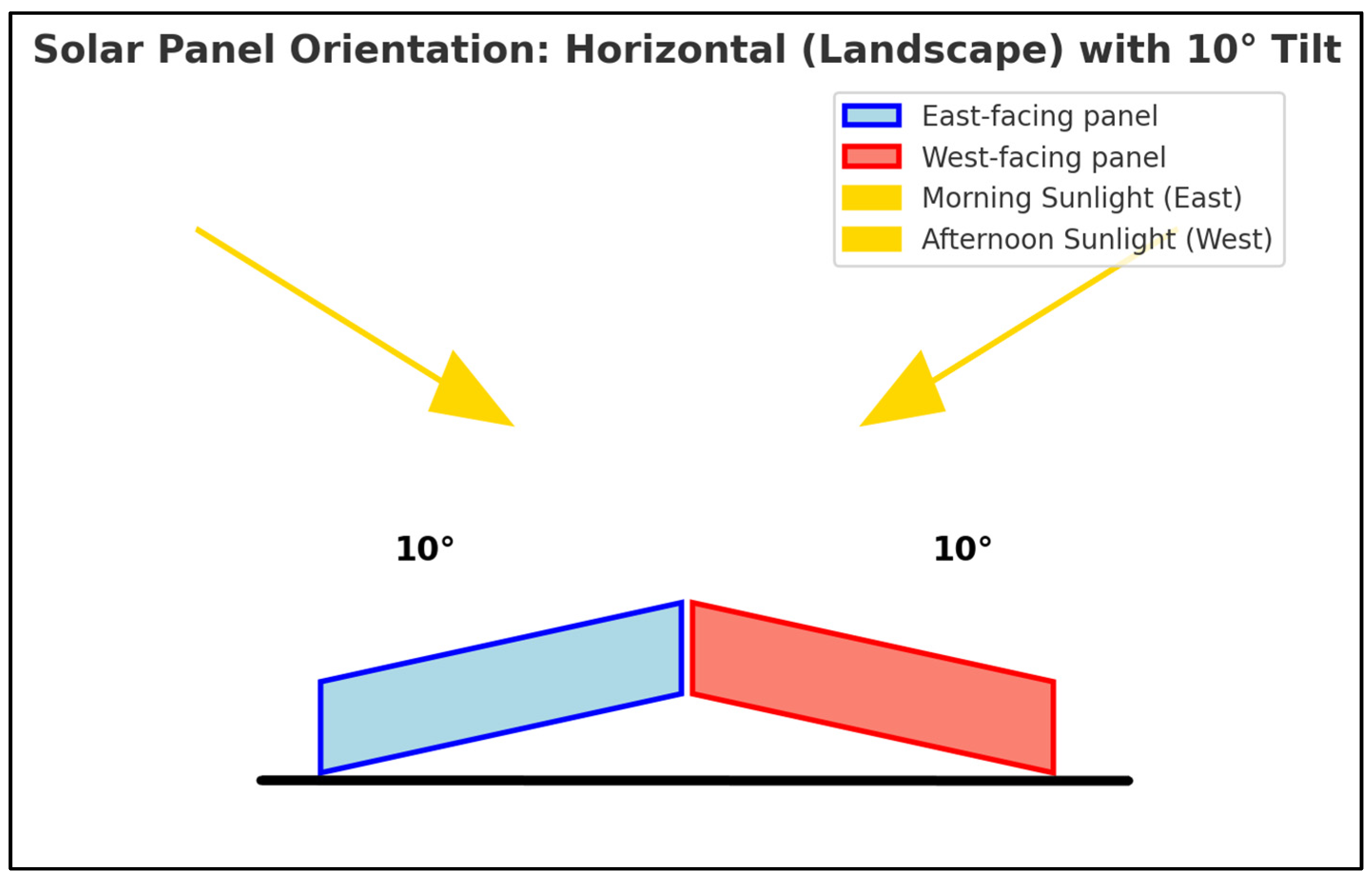
• Electrical protections, cabling, equipment distances, and a tilt angle of 10 degrees were kept constant across all three systems.
• The variable of interest in this study was the orientation of the solar panels. Sets 1 (W1) and 2 (W2) were oriented to the west, while set 3 (E) was oriented to the east. All panels were installed in a landscape configuration with a fixed tilt angle of 10 degrees to optimize energy capture in this equatorial region. Figure 2 shows the arrangement of the solar panels in the experimental setup.

2.3. Data and Measurement Tools

Energy production data (in kWh) was collected over a one-year period, from 1 June 2021, to 31 May 2022. The data collection was performed using a Fronius Data Manager and a Fronius Smart Meter, which recorded real-time data and stored it in the cloud. The historical data were retrieved using the Fronius Solar Web platform.

2.4. Experimental Design

The experiment was conducted using a randomized block design with replicates [33], where each month constituted a block, and daily energy production measurements served as replicates within these blocks. The variables under study include photovoltaic energy production (kWh) as the dependent variable, azimuth angle (east vs. west) as the independent variable, and time (monthly data collection) as the blocking variable. Daily measurements within each month were treated as replicates. The three solar panel systems (W1, W2, and E) were defined as the experimental units.

The three photovoltaic systems were installed on the same rooftop under identical environmental conditions. Systems W1 and W2 were oriented to the west, while system E was oriented to the east, all with a fixed tilt angle of 10°. Each system was equipped with monocrystalline solar panels of the same manufacturer and power rating and connected to identical inverters.

Energy production data were recorded at 5 min intervals using a centralized monitoring system with calibrated sensors and data loggers. To ensure consistency across the experimental units, electrical protections, cable lengths, and installation heights were standardized. This setup enabled a rigorous comparison of energy output based solely on azimuth orientation, eliminating confounding factors related to system design or environmental variability.

2.5. Statistical Analysis Methods

Descriptive analysis: A comprehensive descriptive analysis was conducted, presenting key statistics for each system’s indicators, which included the total annual sum (∑x_i), mean (X), median (M), standard deviation (SD), minimum (min x_i), maximum (max x_i), range (R), skewness (g₁), and kurtosis (g₂). These metrics provide an in-depth understanding of central tendencies and variability in energy production.

• Shapiro–Wilk test: This test was applied to examine the normality of the energy production distributions from each panel. The resulting p-values indicated that the distributions were not normally distributed [34].
• Levene’s test: This test was used to assess the homogeneity of variances between the systems. The results showed no significant differences in variances between the systems with similar orientations [35].
• Central limit theorem: Despite the observed non-normality, the large sample size allowed for the sample mean distribution to approximate normality, relaxing the normality assumption in the statistical inference [36].
• One-way ANOVA: This was performed to determine if there were significant differences in energy production between the different solar panel systems. The analysis revealed no significant differences in the mean energy production among the systems [37].
• Kruskal–Wallis test: Implemented as a non-parametric alternative, this test confirmed the absence of significant differences in the median energy production among the groups [38].
• Randomized block design with replication and two-way ANOVA: This analysis was conducted to account for seasonal variations and azimuth angle. It allowed for the evaluation of both main effects and interactions [37].
• Bonferroni adjustment: This was applied to the p-values obtained from the monthly Kruskal–Wallis analysis to control for Type I errors due to multiple comparisons [39].

2.6. Data Analysis Procedures

Given the nature of the experiment and the daily collection of energy production data, a randomized block design with replication was deemed the most appropriate statistical approach. In this design, each month was defined as a specific block. Within these monthly blocks, each set of solar panels was considered a unit of analysis, and daily values were collected for each set, with the daily measurements acting as replicates within the monthly block. This organization allowed for a detailed examination of daily and monthly variability in energy production, facilitating a more granular analysis of how orientation affects energy performance under different seasonal conditions.

In the analysis phase, we began with descriptive analyses, examining the behavior of energy production for each system as well as seasonal patterns. Subsequently, using a one-way ANOVA (solar panel system), we evaluated whether orientation had a statistically significant effect on energy production over the entire study period. Finally, using a two-way ANOVA (solar panel system and month), we examined whether there were significant interactions between these factors and how they influenced energy production in different months of the year. The R (version 4.4.2.) statistical software was used for all analyses, with a significance level of 0.05 applied to all statistical tests. The extensive amount of data collected and the nature of the experiment led us to consider an ANOVA as the most suitable statistical method, provided that the necessary assumptions were met. The review of these assumptions is discussed throughout the analysis.

To ensure transparency and facilitate a thorough review of our methods and results, detailed tables and supplementary analyses have been included.

3. Results

3.1. Solar Energy Production

The energy production from the solar photovoltaic systems is presented in

Table 1. Solar energy production by system studied.

Month	W1 (West) Production (kWh)	W2 (West) Production (kWh)	E (East) Production (kWh)
June	1527.72	1525.25	1475.08
July	1351.64	1351.29	1337.25
August	1200.43	1198.67	1197.92
September	1833.41	1829.14	1838.85
October	2205.61	2199.99	2253.80
November	2036.65	2025.45	2158.63
December	2105.62	2094.65	2198.26
January	1997.26	1999.14	2084.71
February	1679.81	1691.50	1712.32
March	1711.78	1708.58	1699.05
April	1912.71	1906.94	1846.65
May	2039.87	2035.86	1875.66
Year	21,602.51	21,566.47	21,678.19

. The accumulated annual data reveal that the west-facing panels (W1 and W2) achieve similar energy production, with total annual values of 21,602.51 kWh and 21,566.47 kWh, respectively. In contrast, the east-facing system (E) shows a slight advantage, with a total annual production of 21,678.19 kWh. This marginal difference suggests that, under the specific conditions of this study, the east orientation may offer a slight advantage in terms of annual solar energy capture.

When analyzing the month-by-month data, fluctuations in production reflect the interaction between azimuth angle and seasonal variables, such as solar radiation intensity and day length, as shown in Figure 3. For instance, the months between October and December stand out with significantly higher energy production in the east-facing orientation, possibly indicating a more favorable alignment with the solar incidence angle during these periods. Energy production fluctuates over time, which could indicate seasonal variations or environmental conditions affecting the efficiency of solar panels.

In Figure 3, the variation in annual energy production for the three systems under study can be observed. All lines follow a similar trend, suggesting that these external factors affect the panels similarly. It can be seen that W1 and W2, with similar orientation, show very close production patterns, as evidenced by the tight tracking of the red and blue lines. This indicates consistent production between systems with the same orientation. The green line, corresponding to E, follows a similar pattern, but with slight deviations at certain points, suggesting that the production might be influenced by its different orientation or by other factors not captured by W1 and W2.

A notable drop in production for all three systems is observed around February 2022 (22-02), followed by a recovery in March (22-03). This dynamic could be related to specific weather conditions during that period or other seasonal factors. Unlike in temperate regions, seasonality in Loja is driven more by precipitation and cloud cover than by variations in solar declination. The highest energy production occurs from September to December, corresponding to the dry season, while lower values from February to April are due to increased cloudiness during the rainy season. Overall, Figure 3 provides a visual representation of how energy production changes over time and suggests that azimuth angle may have an effect on the consistency of energy production, although this effect is subtle given the close tracking of the three lines.

Additionally, an analysis of average hourly energy production per month was conducted to better understand diurnal variations and their relationship with energy demand. Figure 4 illustrates the hourly energy production pattern for each month, from June 2021 to May 2022.

As Figure 4 shows, energy production follows a typical diurnal curve, peaking around noon and decreasing during the early morning and late evening hours. Optimal production hours range from 8:00 to 16:00, with maximum generation occurring between 11:00 and 14:00. In contrast, production is low or nonexistent before 7:00 and after 18:00 due to the absence of solar radiation. This daily cycle emphasizes the mismatch between peak solar production and the typical peaks in electricity demand, which often occur in the early morning and evening hours.

3.2. Energy Production Estimation

To validate the observed energy production results, we calculated the theoretical energy yield using the standard PV system energy estimation equation [40]:

$$E_{anual}=P_{STC}\times H_{PSH}\times PR\times 365$$

(1)

where E_anual is the annual energy yield (kWh/year), P_STC is the installed power of the PV system under standard test conditions (kWp), H_PSH is the average daily peak sun hours at the site (h/day), PR is the performance ratio of the system (typically 0.70–0.85), and there are 365 days in a year.

For this study, the installed capacity was 18.225 kWp (45 panels × 405 W), the average PSH for Loja was 5 h/day, and the performance ratio was estimated at 0.75 based on typical system losses. Applying the formula, we obtained the following:

$$E_{anual}=18.225\times 5.0\times 0.75\times 365=24944.64 \mathrm{kWh}/\mathrm{year}$$

This value was used as a reference to compare the real production data obtained from the three systems (east- and west-facing). The real energy yield was consistently lower by approximately 13%, as shown in

Table 2. Difference between projected and actual production.

	Projected Production (kWh)	Actual Production (kWh)	Difference (kWh)	Difference (%)
Actual Production E	24,944.64	21,678.19	3266.45	−13.09
Actual Production W1	24,944.64	21,602.51	3342.13	−13.40
Actual Production W2	24,944.64	21,602.51	3342.13	−13.40

. This difference is attributed to environmental factors, soiling losses, and system inefficiencies not fully captured in the theoretical model.

3.3. Uncertainty Analysis

Uncertainty in experimental results can be due to various factors, such as sensor handling, operating practices, and environmental conditions. This study considers the uncertainty of the inverters. The photovoltaic systems used in this study are equipped with Fronius Symo 15.0-3 208 inverters (Fronius, Monterrey, Mexico). According to their technical specifications, these devices have an estimated relative uncertainty of ±3% in power and energy measurements. This uncertainty is primarily due to the accuracy of the current and voltage sensors integrated into the inverters. The total combined uncertainty was calculated using the uncertainty propagation method [41,42]. For a system composed of multiple independent elements, the combined uncertainty (U_c) is determined by taking the square root of the sum of the individual variances (U_i):

$$U_c=\sqrt{U_1^2+U_2^2+U_3^2}$$

(2)

In this case, three photovoltaic systems (two west-facing and one east-facing) with independent measurements were considered. The results of the uncertainty analysis for each inverter and for the system as a whole are summarized in

Table 3. Energy production (annual) measured by each inverter and the entire system, with their estimated uncertainties.

Element	Measured Energy	Uncertainty (±kWh)	Uncertainty (±%)
Investor 1 (W1)	21,602 kWh	±648 kWh	±3.0%
Investor 2 (W2)	21,566 kWh	±647 kWh	±3.0%
Investor 3 (E)	21,678 kWh	±650 kWh	±3.0%
Total System	64,847 kWh	±1120 kWh	±1.7%

. The expanded uncertainty (≈95% confidence) is reported both in absolute value (energy) and as a relative percentage of the energy produced.

Since each inverter has a relative uncertainty of ±3%, the total combined uncertainty is reduced due to the effect of statistical averaging, resulting in a value of ±1.7% (±1.12 MWh) for the entire system. This lower percentage uncertainty, compared to 3% for each investor, reflects that combining three independent measurements improves confidence in the aggregate value: individual errors tend to be partially offset by the sum of them.

4. Discussion

4.1. Descriptive Analysis

The statistical analysis of energy production in relation to the orientation of the solar panels is presented in

Table 4. Descriptive statistics by group of solar panels studied.

Parameter	W1	W2	E
Number of observations (n)	365	365	365
Sum (∑xi)	21.603	21.566	21.678
Mean (X)	59.18	59.09	59.39
Median (M)	58.18	58.10	59.07
Standard deviation (SD)	20.04	20.00	20.90
Min (min xi)	14.10	14.14	14.34
Max (max xi)	110.42	110.23	112.49
Range (R)	96.32	96.08	98.15
Skew (g1)	0.12	0.12	0.19
Kurtosis (g2)	−0.49	−0.48	−0.48

. Through daily records over one year, 365 measurements were obtained for each orientation, allowing for a robust analysis based on a complete and representative dataset.

The accumulated production values (sum, ∑x_i) show a subtle divergence between orientations, with totals of 21,603 kWh for W1 and 21,566 kWh for W2, both west-oriented, compared to 21,678 kWh for E, east-oriented. Although this difference is small, it highlights the influence of orientation on solar energy capture.

The mean (X) and median (M) provide insight into the central tendency of the data, with slightly higher values for the east orientation (E), indicating a higher daily average production and a superior midpoint in distribution compared to the west-facing orientations. This could be interpreted as greater consistency in the energy production of east-facing panels.

The variability analysis, measured through the standard deviation (SD), shows comparable dispersion between the west orientations, but slightly higher in the east orientation. This may suggest the influence of additional environmental or systematic factors affecting production variability in the east orientation.

The extreme values, indicated by the minimum (min x_i) and maximum (max x_i) parameters, along with the range (R), show the full amplitude of energy production, which is slightly higher in the east orientation. Such amplitude may indicate days of exceptionally high or low production, influenced by seasonality and the inherent intermittency of solar energy.

The skewness (g₁) of the datasets is positive in all cases, indicating a distribution with a heavier tail toward higher production values. The kurtosis (g₂), close to zero, suggests that the distributions do not deviate significantly from normality in terms of “peakedness”.

Therefore, this analysis affirms that the orientation of solar panels has a detectable impact on electricity production, although the magnitude of this impact is relatively modest, as indicated by the statistical parameters. These findings underscore the importance of considering orientation in the design and planning of photovoltaic installations to optimize energy efficiency. However, further studies incorporating a broader range of geographical and climatic conditions are important to generalizing and validating these preliminary observations.

4.2. Influence of Azimuth Angle on Energy Production

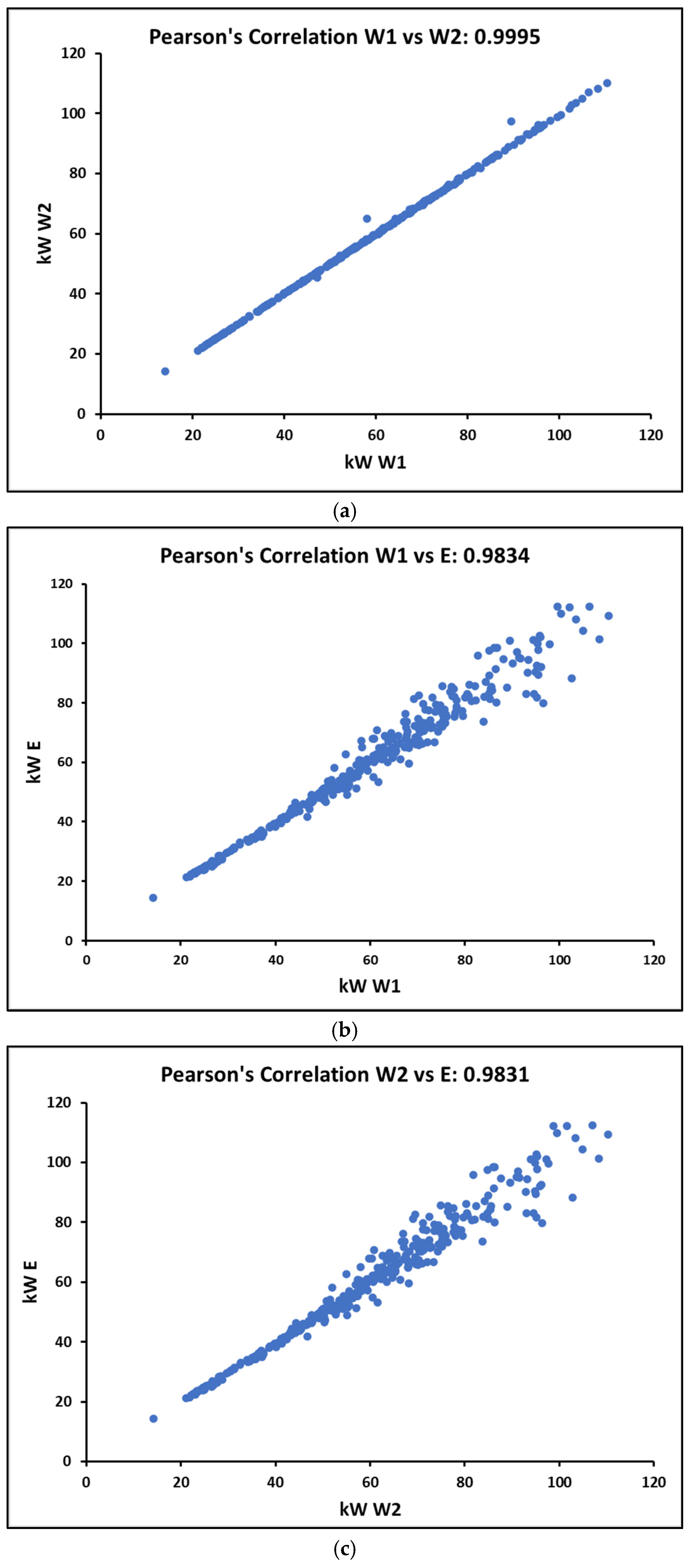
4.2.1. Correlation Evaluation

The evaluation of the correlation between energy production from solar panel systems with different orientations is presented in Figure 5a–c.

In Figure 5a, the Pearson correlation coefficient (r) between sets W1 and W2 is 0.99995, indicating a strong linear relationship between the production of these panel sets. Given that these panels share technical specifications and have similar orientations, this result was expected and validates the internal consistency of the data and the homogeneity of operating conditions.

Figure 5b,c, comparing W1 and W2 with E, respectively, show slightly lower correlations of 0.9834 and 0.9831. Although these figures still represent strong correlations, the broader dispersion of the data points suggests additional factors may be influencing E production. Considering that E has a different orientation than W1 and W2, these results support the hypothesis that orientation has a noticeable effect on energy production.

While the variability in the E data is more pronounced, it is not significant enough to challenge the overall trend that the azimuth angle of the solar panel affects and does not dramatically redefine energy production capacity. Thus, the data presented in these graphs confirm the impact of orientation on solar energy generation efficiency and support its consideration as a factor in the design and planning of photovoltaic systems. This detailed understanding is vital for advancing toward more efficient and optimized energy infrastructure.

4.2.2. One-Way ANOVA

The detailed results of the normality test and variance equality test are presented in

Table 5. Results (p values) of the normality (Shapiro–Wilk) and equality of variances (Levene) tests for the total data in each panel.

Test	Shapiro–Wilk	p-Value (Shapiro–Wilk)	Levene	p-Value (Levene)
W1	✓	0.00554	-	-
W2	✓	0.00514	-	-
E	✓	0.00199	-	-
W1/W2	-	-	✓	0.9611
W1/E	-	-	✓	0.3218
W2/E	-	-	✓	0.2985

Note: In this combined table, we specify which values belong to the Shapiro–Wilk test and which to the Levene test, using separate columns to clarify that some rows refer to normality tests (Shapiro–Wilk) and others to homogeneity of variance tests (Levene). Spaces marked with “-” indicate that, for that row, the category does not apply.

.

Applying the Shapiro–Wilk test (W), we found significantly low p-values, p = 0.00554, 0.00514, and 0.00199 for systems Si1, Sib, and E, respectively, suggesting the rejection of the null hypothesis of normal distribution for the energy production data of each group. This indicates that energy production does not follow a Gaussian distribution, which could be indicative of non-random external influences affecting the systems, possibly related to orientation.

Additionally, Levene’s test was applied to examine the homogeneity of variances, a key premise in comparing group means. The resulting p-values for comparisons between W1/W2, W1/E, and W2/E (0.9611, 0.3218, and 0.2985, respectively) indicate that we cannot reject the null hypothesis of equal variances between groups with similar orientations (W1 and W2), while there is a tendency toward heterogeneity when comparing these with E.

Despite the violation of the normality assumption, the large sample size (365 observations per system) allows us to invoke the central limit theorem, which holds that the distribution of the sample mean will tend toward normality as the sample size increases. This enables us to relax the normality assumption for statistical inference.

ANOVA results did not show significant differences in energy production between the systems (F = 0.022, p = 0.979), as presented in

Table 6. Principal components of the analysis of variance (ANOVA).

Source	Df	Sum Sq	Mean Sq	F Value	Pr (>F)
Systems	2	18	8.9	0.022	0.979
Residuals	1092	450,787	412.8	-

Note: This table summarizes the principal components of the analysis of variance (ANOVA) for the “Systems” factor and the residuals, including the degrees of freedom (Df), the sum of squares (Sum Sq), the mean of the squares (Mean Sq), the F value, and the probability of obtaining an F value greater than that observed under the null hypothesis (Pr (>F)). Note that the “F value” and “Pr (>F)” values apply only to the “System” factor, as these values are not calculated for the residuals in a typical ANOVA analysis.

, indicating that orientation does not significantly influence mean energy production. This result is consistent with previous descriptive analyses and suggests an absence of a significant effect of orientation on energy production.

Given the violation of the normality assumption, the Kruskal–Wallis test was applied as a precautionary measure (

Table 7. Kruskal–Wallis test.

Test	Statistic	Df	p-Value
Kruskal–Wallis chi-squared	0.009878	2	0.9951

Note: This table shows the result of the Kruskal–Wallis test for the comparison between groups defined by “Panel”. It includes the test statistic (“Kruskal–Wallis chi-squared”), the degrees of freedom (Df), and the p value associated with the test, which indicates the probability of obtaining a test statistic at least as extreme as that observed under the null hypothesis that all group distributions are equal.

), resulting in a p-value of 0.9951. This further supports the ANOVA conclusion, indicating no significant differences in median energy production between the groups.

4.2.3. Randomized Block Design with Replication

Following the experimental design of the randomized block design with replication, we applied a two-way ANOVA to examine how azimuth angle and seasonal variations affect energy production. This analysis, incorporating both the “System” and “YearMonth” factors, allowed us to delve deeper into the dynamics between azimuth angle and monthly changes in energy generation (

Table 8. Results of the two-factor ANOVA.

	Df	Sum Sq	Mean Sq	F Value	Pr (>F)
Panel	2	18	9	0.028	0.973
YearMonth	11	110,166	10,015	31.276	<2 × 10−16
System–YearMonth	22	1515	69	0.215	1.000
Residuals	1059	339,106	320	-	-

).

From Table 6, the main effects and interactions observed are as follows:

• System: The absence of statistically significant differences in energy production between the solar panel systems (F = 0.028, p = 0.973) reinforces our initial conclusion that the specific orientation of the panels does not significantly influence their energy performance.
• YearMonth: The significant monthly variation in energy production (F = 31.276, p < 2 × 10⁻¹⁶) highlights the impact of seasonality, an expected result given the sun-dependent nature of solar energy.
• System–YearMonth interaction: The lack of significant interaction (F = 0.215, p = 1.000) suggests that seasonal differences in energy production do not depend significantly on the orientation of the solar panel systems. In other words, while energy production varies by month, this variation is consistently similar across the different systems.

These findings suggest that, under the study conditions, the azimuth angle does not differentially impact energy production throughout the year. Seasonal variation (which is significant, as shown in the main effect of YearMonth) acts independently of the panel system used. This means that all systems respond similarly to seasonal variations.

Although the initial check for the one-way ANOVA analysis verified the fulfillment of its assumptions, the incorporation of the “month” factor required an additional verification.

Table 9. Shapiro–Wilk test for normality.

#	Panel	Year/Month	p-Value	Statistic
1	W1	21-06	0.274	0.958
2	W1	21-07	0.0850	0.940
3	W1	21-08	0.00277	0.883
…	…	…	…	…
34	E	22-03	0.0507	0.932
35	E	22-04	0.311	0.960
36	E	22-05	0.251	0.958

Note: The Shapiro–Wilk table has been abbreviated to keep the response concise, but all records follow a format similar to those shown. This organization allows easy viewing of both the results of the homogeneity of variances test (Levene) and the normality test (Shapiro–Wilk), including the statistical significance of the findings.

details the results of the normality and variance equality tests for all possible combinations (groups) of the System and Month levels.

Levene’s test revealed a violation of the homogeneity of variances assumption (p = 0.03605) among these groups, prompting us to proceed with greater caution in our analysis. Likewise, the normality evaluation showed that not all groups conformed to a normal distribution. These observations supported our decision to apply the non-parametric Kruskal–Wallis test for each month, providing a more appropriate method given the non-conformity with the standard ANOVA assumptions [43].

The application of the Kruskal–Wallis test for monthly analysis (

Table 10. Kruskal–Wallis test results for median differences by month.

#	Month	KW Statistic	p-Value	p Bonferroni
1	21-06	0.608644689	0.7376231	1
2	21-07	0.106272278	0.9482509	1
3	21-08	0.031970244	0.9841420	1
4	21-09	0.025006105	0.9875748	1
5	21-10	0.406314345	0.8161500	1
6	21-11	2.897094017	0.2349114	1
7	21-12	0.469457790	0.7907852	1
8	22-01	0.344676423	0.8416945	1
9	22-02	0.006842737	0.9965845	1
10	22-03	0.047114043	0.9767183	1
11	22-04	0.189401709	0.9096450	1
12	22-05	2.077357363	0.3539220	1

Note: Table with the results of the Kruskal–Wallis test for differences in medians for each month, including the Kruskal–Wallis statistic, the p-value, and the Bonferroni adjustment for the p-value. This table summarizes the results of the Kruskal–Wallis test performed for each month, looking for significant differences in the medians. The Bonferroni adjustment for the p-value has been applied, but in all cases, it has resulted in a value of one, indicating that no statistically significant differences have been found after the adjustment.

), based on the violation of the normality and homogeneity of variance assumptions, confirmed the absence of significant differences in energy production between the panels at the monthly level (p-values > 0.05 for all months). To ensure rigor in the face of multiple comparisons and minimize the risk of Type I errors, a Bonferroni adjustment was applied to the obtained p-values. This adjustment, known for its conservative approach, reaffirmed the absence of significant differences after a stricter review of the results (Bonferroni-adjusted p-values > 0.05 for all months). Despite the seasonal variability, the azimuth angle does not significantly affect their energy performance.

Both the two-way ANOVA and the subsequent monthly Kruskal–Wallis tests confirmed that azimuth angle does not have a significant impact on energy generation. This consistent result, even after conservative adjustments for multiple tests, underscores the consistency in the response of systems to seasonal variations, regardless of their orientation.

4.3. Uncertainty Calculation

Regarding the total uncertainty calculation, it was determined that each Fronius Symo 15.0-3 208 inverter exhibits an approximate uncertainty of ±3.0% in its daily or annual energy measurement. This percentage is primarily due to the tolerances of its current and voltage sensors, according to independent technical tests reported in the manufacturer’s data sheet. The uncertainty of the entire system, consisting of the three inverters, is lower and is estimated at approximately ±1.7%, thanks to the combination of independent measurements. This value implies that the measured annual total, close to 64.8 MWh, could vary by ±1.1 MWh due to the combined instrumental uncertainty.

The results in Table 3 facilitate the understanding of the magnitudes of uncertainty involved. For example, inverter W1, with approximately 21,600 kWh, has a possible error of ±648 kWh, while the entire system with 64,800 kWh has a margin of error of ±1120 kWh. In relative terms, the entire system offers greater overall certainty (±1.7%) than each individual component (±3%). These results highlight the importance of considering uncertainty in evaluating the performance of photovoltaic systems. Although modern inverters provide highly accurate data, there is always a margin of error. The analyzed solar system shows consistent behavior, and the recorded data are reliable within a well-defined uncertainty range.

4.4. Comparison of Results of This Study with Others Reported in the Literature

The comparison of studies on azimuth and tilt angles in various regions, reflected in

Table 11. Comparison of results of this study with the literature.

Location	Key Findings	Implications	Ref.
Global	South-facing orientation maximizes efficiency in higher latitudes	Orientation adjustments are less impactful in equatorial regions due to consistent solar path	[1]
Switzerland	West orientation better aligns with daily demand	Orientation adjustments based on demand patterns improve grid performance	[2]
Temperate Regions	Minor deviations from optimal orientation do not significantly affect energy yield	Tilt and azimuth adjustments critical in temperate climates for maximizing output	[11]
Romania	Seasonal tilt adjustments increase energy capture by up to 4.8%	Seasonal tilt adjustments are crucial for maximizing output in colder climates	[12]
USA	South orientation with tilt equal to local latitude maximizes energy	Orientation and tilt adjustments are location-specific for optimizing yield	[13]
Morocco	Best performance in landscape orientation	Orientation critical for maximizing output in semi-arid climates	[14]
Equatorial Areas	Orientation variations have less impact due to consistent solar path	Stable solar path minimizes the impact of orientation in equatorial regions	[15]
Turkey	Maximum energy generation achieved with 31.33° tilt angle	Focus on specific tilt for optimizing generation in agrivoltaic systems	[18]
Iceland, Canada, Ecuador, and Brazil	Biannual reorientation improves output by 3–4.8%	Biannual adjustments optimize energy production in varying climates	[19]
Equatorial Regions	Optimal tilt angles close to latitude, requiring minimal seasonal adjustments	Supports minimal tilt adjustments in equatorial regions	[20]
General Analysis	East–west orientations support similar energy production to traditional setups	Orientation adjustments are less critical in consistent solar conditions	[23]
Various Regions	East–west orientations reduce storage needs by matching demand patterns	East–west setups improve demand alignment and reduce storage needs	[28]
Netherlands and Germany	Optimal orientation varies with demand patterns; 212° azimuth and 26° tilt maximize self-consumption	Demand-based orientation adjustments necessary for maximizing self-consumption	[29]
Equatorial Regions	Slight advantage for east-facing panels in October–November	Solar altitude variations affect panel performance seasonally	[44]
General Analysis	Emphasizes need for dual-axis tracking and tilt optimization	Dual-axis tracking and advanced tilt control needed for further optimization	[45]
Turkey	Monthly optimal tilt varies between 13° and 61°	Seasonal adjustments critical for optimizing output	[46]
Indonesia	Higher annual energy yield with north-facing orientation but increased uncertainty	Orientation impacts uncertainty and energy yield in tropical regions	[47]
India	Direct relation between irradiance and energy generation with optimal tilt close to latitude	Tilt adjustments based on irradiance critical for maximizing output	[48]
Southern Ecuador	Minimal differences in energy output between east- and west-facing orientations	Focus on other factors like cost, installation, and maintenance for PV optimization	This study

, highlights the importance of adjusting these parameters according to geographic and climatic conditions.

Studies conducted in equatorial regions indicate that panel orientation has little impact on energy production, owing to the stable and consistent solar trajectory throughout the year. In these areas, minor tilt adjustments are generally sufficient to optimize annual energy capture. In contrast, higher-latitude regions require seasonal adjustments in tilt and azimuth angles, especially in winter, where optimal tilting can increase solar absorption by up to 4.8%.

This study confirms that in southern Ecuador, the differences between east- and west-facing panels are minimal, reinforcing the notion that azimuth angle is less critical under stable solar conditions. Consequently, economic and logistical criteria can be prioritized in PV system design without significant energy loss.

However, orientation should not be based solely on total energy yield. When evaluating grid-connected or off-grid systems, it is essential to consider daily demand patterns. As highlighted by Mubarak et al. (2019) [49], east–west PV configurations help to distribute energy generation more evenly throughout the day, aligning better with consumption peaks in the morning and evening. This approach can reduce the need for energy storage, which, although becoming more accessible, still involves additional costs.

4.5. Opportunities for Future Research

The findings demonstrate that seasonal variations have a more significant impact on energy production than azimuthal orientation, suggesting that, in equatorial regions, practical considerations such as structural constraints, economic factors, and logistical ease can be prioritized over azimuth optimization without significantly sacrificing efficiency. This provides valuable information for optimizing the design of photovoltaic systems in areas where solar energy use remains underdeveloped.

While this study provides valuable insights into the performance of PV systems with different azimuth orientations in an equatorial setting, several opportunities remain for future research. Extending the monitoring period beyond one year would allow for the evaluation of interannual climate variability. Exploring the effect of adjustable tilt angles could help optimize seasonal energy capture. Conducting similar studies in other tropical regions with varying altitudes, humidity, or cloud patterns would improve the generalizability of results. Additionally, integrating energy demand profiles would support the assessment of alignment between production and consumption, which is essential for evaluating storage requirements and system efficiency in both grid-connected and off-grid contexts.

5. Conclusions

This one-year study, supported by rigorous statistical analyses, conducted in an equatorial location (Loja, Ecuador) demonstrates that, for a fixed tilt angle of 10°, the geographic orientation of photovoltaic (PV) panels has a minimal impact on annual energy production. The difference in cumulative energy yield between east- and west-facing panels was less than 1%, confirming that both configurations perform similarly under equatorial solar conditions.

The analysis of diurnal variations revealed that energy production follows a typical daily curve, peaking around midday and declining during early morning and late evening hours. This pattern highlights a mismatch between peak solar production and typical electricity demand, which often occurs in the morning and evening. Future studies should integrate energy demand profiles to optimize PV system design and improve alignment with consumption patterns.

These results indicate that, in regions near the equator, PV azimuth angle can be selected based on non-irradiance factors, such as space constraints, structural feasibility, or energy consumption patterns, without significant losses in total energy generation. Additionally, observed variations in energy production throughout the year were primarily attributed to environmental and seasonal factors, including changes in cloud cover, atmospheric conditions, and temperature fluctuations. Future research should incorporate multi-year energy production data and historical weather records to assess the long-term consistency of these fluctuations and further refine photovoltaic system optimization strategies for equatorial locations.

These findings provide valuable insights for solar energy system design in equatorial regions, reinforcing that fixed installations with a low tilt angle can be oriented flexibly without major efficiency losses. The results can serve as a technical reference for urban, residential, and commercial photovoltaic projects in similar climates, guiding decision-making processes in renewable energy deployment.

References

1. Izam, N.S.M.N.; Itam, Z.; Sing, W.L.; Syamsir, A. Sustainable Development Perspectives of Solar Energy Technologies with Focus on Solar Photovoltaic—A Review. Energies 2022, 15, 2790. [Google Scholar] [CrossRef]
2. Middelhauve, L.; Baldi, F.; Stadler, P.; Maréchal, F. Grid-Aware Layout of Photovoltaic Panels in Sustainable Building Energy Systems. Front. Energy Res. 2021, 8, 573290. [Google Scholar] [CrossRef]
3. Liu, W.; Wang, J.; Wang, Y. Building solar integrated energy systems considering power and heat coordination: Optimization and evaluation. Sol. Energy 2024, 279, 112821. [Google Scholar] [CrossRef]
4. Maka, A.O.M.; Alabid, J.M. Solar energy technology and its roles in sustainable development. Clean Energy 2022, 6, 476–483. [Google Scholar] [CrossRef]
5. Bassam, N. El Solar energy. In Distributed Renewable Energies for Off-Grid Communities: Empowering a Sustainable, Competitive, and Secure Twenty-First Century; Elsevier: Amsterdam, The Netherlands, 2021; pp. 123–147. ISBN 9780128216057. [Google Scholar]
6. Dambhare, M.V.; Butey, B.; Moharil, S.V. Solar photovoltaic technology: A review of different types of solar cells and its future trends. J. Phys. Conf. Ser. 2021, 1913, 012053. [Google Scholar] [CrossRef]
7. Tapia, M.; Ramos, L.; Heinemann, D.; Zondervan, E. Power to the city: Assessing the rooftop solar photovoltaic potential in multiple cities of Ecuador. Phys. Sci. Rev. 2023, 8, 2285–2319. [Google Scholar] [CrossRef]
8. Icaza, D.; Borge-Diez, D.; Galindo, S.P. Analysis and proposal of energy planning and renewable energy plans in South America: Case study of Ecuador. Renew. Energy 2022, 182, 314–342. [Google Scholar] [CrossRef]
9. Barragán-Escandón, A.; Jara-Nieves, D.; Romero-Fajardoc, I.; Zalamea-Leónesteban, E.F.; Serrano-Guerrero, X. Barriers to renewable energy expansion: Ecuador as a case study. Energy Strateg. Rev. 2022, 43, 100903. [Google Scholar] [CrossRef]
10. Benalcazar, P.; Lara, J.; Samper, M. Distributed Photovoltaic Generation in Ecuador: Economic Analysis and Incentives Mechanisms. IEEE Lat. Am. Trans. 2020, 18, 564–572. [Google Scholar] [CrossRef]
11. Phadnis, N.; Yang, R.J.; Wijeratne, P.U.; Zhao, H.; Liu, C. The Impact of Solar PV Design Tilt and Orientation on Project Values. Smart Innov. Syst. Technol. 2019, 131, 301–310. [Google Scholar] [CrossRef]
12. Danu, A.; Tanasiev, V.; Ionescu, C.; Badea, A. Influence of tilt and orientation angle of the PV panels on high-energy production in Romanian climate conditions during cold season. In Proceedings of the 2015 IEEE 15th International Conference on Environment and Electrical Engineering, EEEIC 2015-Conference Proceedings, Rome, Italy, 10–13 June 2015; Institute of Electrical and Electronics Engineers Inc.: Piscataway, NJ, USA, 2015; pp. 1599–1604. [Google Scholar]
13. Naraghi, M.H.; Atefi, E. Optimum Solar Panel Orientation and Performance: A Climatic Data-Driven Metaheuristic Approach. Energies 2022, 15, 624. [Google Scholar] [CrossRef]
14. Oufettoul, H.; Lamdihine, N.; Motahhir, S.; Lamrini, N.; Abdelmoula, I.A.; Aniba, G. Comparative Performance Analysis of PV Module Positions in a Solar PV Array Under Partial Shading Conditions. IEEE Access 2023, 11, 12176–12194. [Google Scholar] [CrossRef]
15. Yadav, S.; Panda, S.K.; Hachem-Vermette, C. Optimum azimuth and inclination angle of BIPV panel owing to different factors influencing the shadow of adjacent building. Renew. Energy 2020, 162, 381–396. [Google Scholar] [CrossRef]
16. Guo, S.-t.; Liu, J.; Qian, W.; Zhu, W.-h.; Zhang, C.-y. A review of quantum chemical methods for treating energetic molecules. Energ. Mater. Front. 2021, 2, 292–305. [Google Scholar] [CrossRef]
17. Peng, H.Y.; Shen, Z.; Liu, H.J.; Dai, S.F. Wind loads on rooftop solar photovoltaic panels oriented with varying azimuth angles: A comprehensive wind tunnel analysis. J. Build. Eng. 2024, 92, 109747. [Google Scholar] [CrossRef]
18. Kallioğlu, M.A.; Avcı, A.S.; Sharma, A.; Khargotra, R.; Singh, T. Solar collector tilt angle optimization for agrivoltaic systems. Case Stud. Therm. Eng. 2024, 54, 103998. [Google Scholar] [CrossRef]
19. Prunier, Y.; Chuet, D.; Nicolay, S.; Hamon, G.; Darnon, M. Optimization of photovoltaic panel tilt angle for short periods of time or multiple reorientations. Energy Convers. Manag. X 2023, 20, 100417. [Google Scholar] [CrossRef]
20. Alam, S.; Qadeer, A.; Afazal, M. Determination of the optimum tilt-angles for solar panels in Indian climates: A new approach. Comput. Electr. Eng. 2024, 119, 109638. [Google Scholar] [CrossRef]
21. Khatib, A.T.; Samiji, M.E.; Mlyuka, N.R. Optimum Solar Collector’s North-South Tilt Angles for Dar es Salaam and their Influence on Energy Collection. Clean. Eng. Technol. 2024, 21, 100778. [Google Scholar] [CrossRef]
22. Mukisa, N.; Zamora, R. Optimal tilt angle for solar photovoltaic modules on pitched rooftops: A case of low latitude equatorial region. Sustain. Energy Technol. Assess. 2022, 50, 101821. [Google Scholar] [CrossRef]
23. Mahmud, Z.; Kurtz, S. Effect of solar panel orientation and EV charging profile on grid design. Renew. Energy 2024, 231, 120923. [Google Scholar] [CrossRef]
24. Arslan, M.; Çunkaş, M. An experimental study on determination of optimal tilt and orientation angles in photovoltaic systems. J. Eng. Res. 2024; in press. [Google Scholar] [CrossRef]
25. AL-Rousan, N.; AL-Najjar, H. Optimized deep neural network to estimate orientation angles for solar photovoltaics intelligent systems. Clean. Eng. Technol. 2024, 20, 100754. [Google Scholar] [CrossRef]
26. Kerr, J.; Moores, J.E.; Smith, C.L. An improved model for available solar energy on Mars: Optimizing solar panel orientation to assess potential spacecraft landing sites. Adv. Space Res. 2023, 72, 1431–1447. [Google Scholar] [CrossRef]
27. Kabeel, A.E.; Khelifa, A.; El Hadi Attia, M.; Abdelgaied, M.; Arıcı, M.; Abdel-Aziz, M.M. Optimal design and orientation of cooling technology for photovoltaic Plants: A comparative simulation study. Sol. Energy 2024, 269, 112362. [Google Scholar] [CrossRef]
28. Bouguerra, S.; Yaiche, M.R.; Gassab, O.; Sangwongwanich, A.; Blaabjerg, F. The Impact of PV Panel Positioning and Degradation on the PV Inverter Lifetime and Reliability. IEEE J. Emerg. Sel. Top. Power Electron. 2021, 9, 3114–3126. [Google Scholar] [CrossRef]
29. Litjens, G.B.M.A.; Worrell, E.; van Sark, W.G.J.H.M. Influence of demand patterns on the optimal orientation of photovoltaic systems. Sol. Energy 2017, 155, 1002–1014. [Google Scholar] [CrossRef]
30. Li, M.; Liu, Y.; Li, J.; Li, F.; An, Y.; Gao, X. Optimizing sustainable energy integration: A novel approach using concentrated solar plant and hybrid power supply. Electr. Power Syst. Res. 2024, 237, 111050. [Google Scholar] [CrossRef]
31. Sadaq, S.I.; Mehdi, S.N.; Mohinoddin, M. Experimental analysis on solar photovoltaic (SPV) panel for diverse slope angles at different wind speeds. Mater. Today Proc. 2023; in press. [Google Scholar] [CrossRef]
32. Żurakowska-Sawa, J.; Gromada, A.; Trocewicz, A.; Wojciechowska, A.; Wysokiński, M.; Zielińska, A. Photovoltaic Farms: Economic Efficiency of Investments in South-East Poland. Energies 2025, 18, 170. [Google Scholar] [CrossRef]
33. Alvarado, G.; Rodríguez, F.M.; Pacheco, A.; Burgueño, J.; Crossa, J.; Vargas, M.; Pérez-Rodríguez, P.; Lopez-Cruz, M.A. META-R: A software to analyze data from multi-environment plant breeding trials. Crop J. 2020, 8, 745–756. [Google Scholar] [CrossRef]
34. Khatun, N. Applications of Normality Test in Statistical Analysis. Open J. Stat. 2021, 11, 113–122. [Google Scholar] [CrossRef]
35. Wang, Y.; Tang, M.; Wang, P.; Liu, B.; Tian, R. The Levene test based-leakage assessment. Integration 2022, 87, 182–193. [Google Scholar] [CrossRef]
36. Zhang, X.; Astivia, O.L.O.; Kroc, E.; Zumbo, B.D. How to Think Clearly About the Central Limit Theorem. Psychol. Methods 2022, 28, 1427–1445. [Google Scholar] [CrossRef]
37. Okoye, K.; Hosseini, S. Analysis of Variance (ANOVA) in R: One-Way and Two-Way ANOVA. In R Program; Springer: Singapore, 2024; pp. 187–209. [Google Scholar] [CrossRef]
38. Okoye, K.; Hosseini, S. Mann–Whitney U Test and Kruskal–Wallis H Test Statistics in R. In R Program; Springer: Singapore, 2024; pp. 225–246. [Google Scholar] [CrossRef]
39. Kumbure, M.M.; Luukka, P.; Collan, M. A new fuzzy k-nearest neighbor classifier based on the Bonferroni mean. Pattern Recognit. Lett. 2020, 140, 172–178. [Google Scholar] [CrossRef]
40. Abdullah, G.; Nishimura, H. Techno-Economic Performance Analysis of a 40.1 kWp Grid-Connected Photovoltaic (GCPV) System after Eight Years of Energy Generation: A Case Study for Tochigi, Japan. Sustainability 2021, 13, 7680. [Google Scholar] [CrossRef]
41. PraveenKumar, S.; Kumar, A. Thermodynamic, environmental and economic analysis of solar photovoltaic panels using aluminium reflectors and latent heat storage units: An experimental investigation using passive cooling approach. J. Energy Storage 2025, 112, 115487. [Google Scholar] [CrossRef]
42. Hamdan, M.; Abdelhafez, E.; Ajib, S.; Sukkariyh, M. Improving Thermal Energy Storage in Solar Collectors: A Study of Aluminum Oxide Nanoparticles and Flow Rate Optimization. Energies 2024, 17, 276. [Google Scholar] [CrossRef]
43. Selvi, S.; Mohanraj, M.; Duraipandy, P.; Kaliappan, S.; Natrayan, L.; Vinayagam, N. Optimization of Solar Panel Orientation for Maximum Energy Efficiency. In Proceedings of the 2023 4th International Conference on Smart Electronics and Communication (ICOSEC), Trichy, India, 20–22 September 2023; pp. 159–162. [Google Scholar] [CrossRef]
44. Apaolaza-Pagoaga, X.; Carrillo-Andrés, A.; Jiménez-Navarro, J.P.; Ruivo, C.R. Experimental evaluation of the performance of new Copenhagen solar cooker configurations as a function of solar altitude angle. Renew. Energy 2024, 229, 120782. [Google Scholar] [CrossRef]
45. Wei, D.; Basem, A.; Alizadeh, A.; Jasim, D.J.; Aljaafari, H.A.S.; Fazilati, M.; Mehmandoust, B.; Salahshour, S. Optimum tilt and azimuth angles of heat pipe solar collector, an experimental approach. Case Stud. Therm. Eng. 2024, 55, 104083. [Google Scholar] [CrossRef]
46. Kacira, M.; Simsek, M.; Babur, Y.; Demirkol, S. Determining optimum tilt angles and orientations of photovoltaic panels in Sanliurfa, Turkey. Renew. Energy 2004, 29, 1265–1275. [Google Scholar] [CrossRef]
47. Mangkuto, R.A.; Tresna, D.N.A.T.; Hermawan, I.M.; Pradipta, J.; Jamala, N.; Paramita, B.; Atthaillah. Experiment and simulation to determine the optimum orientation of building-integrated photovoltaic on tropical building façades considering annual daylight performance and energy yield. Energy Built Environ. 2024, 5, 414–425. [Google Scholar] [CrossRef]
48. Sameera; Tariq, M.; Rihan, M. Analysis of the impact of irradiance, temperature and tilt angle on the performance of grid-connected solar power plant. Meas. Energy 2024, 2, 100007. [Google Scholar] [CrossRef]
49. Mubarak, R.; Luiz, E.W.; Seckmeyer, G. Why PV Modules Should Preferably No Longer Be Oriented to the South in the Near Future. Energies 2019, 12, 4528. [Google Scholar] [CrossRef]
Figure 1. Flowchart of the methodology used in this study.
Energies 18 01998 g001
Figure 2. Position of the solar panels in the experimental setup. The panels are in landscape configuration with a fixed tilt of 10°, facing east (light blue) and west (light red). The golden arrows represent the direction of solar radiation during each period of the day.
Energies 18 01998 g002
Figure 3. Average daily production of electrical energy (measured in kilowatt hours kWh), from June 2021 to May 2022, for the three groups of solar panels, identified as W1 (west), W2 (west), and E (east).
Energies 18 01998 g003
Figure 4. Average hourly energy production per month (Wh).
Energies 18 01998 g004
Figure 5. Correlation between energy production from solar panel systems with different orientations: (a) W1 vs. W2, (b) W1 vs. E and (c) W2 vs. E. The series of scatter plots presented demonstrate a statistical correlation between the energy production of different solar panels, providing numerical evidence of the influence of orientation on the efficiency of solar energy collection.
Energies 18 01998 g005