Abstract
The aim of this study is to compare the performance of various deep learning models in predicting the arrival and charging time of an electric vehicle at a charging station. The objective is to identify the most precise model capable of predicting the time from the driver’s location to the arrival at the charging station. Initially, an effort was made to ascertain which model type offers superior prediction accuracy, characterized by low error rates and high success scores. To this end, the study examined the prediction capabilities of the LSTM (Long Short-Term Memory), GRU (Gated Recurrent Unit), Prophet, and ARIMA (Autoregressive Integrated Moving Average) models, which were trained with historical data using various metrics. These metrics included the R2 (R-squared)success metric, MAE (Mean Absolute Error) and MSE (Mean Squared Error) error metrics, DTW (Dynamic Time Warping) metric scores, and model selection. In MAE metric scores, GRU has an error rate of 0.38, LSTM 0.50, Prophet 0.61, and ARIMA 2.31. For MSE metric scores, GRU has an error rate of 2.92, LSTM 3.05, Prophet 4.21, and ARIMA 65.54. In R2 metric scores, GRU has a success rate of 0.99, LSTM 0.99, Prophet 0.13, and ARIMA −2.19. In DTW metric scores, GRU has a distance ratio of 125.5, LSTM 126.9, Prophet 185.9, and ARIMA 454.9. Based on these score values, it was decided that the GRU model made the most accurate time estimation. After observing the superior performance of the GRU model, the time prediction capability of this model is demonstrated through an interface program for charging stations in the province of Kocaeli, which serves as the model’s real-world application area. The main contribution of this article is that LSTM, GRU, Prophet, and ARIMA deep learning approaches, which are preferred in many studies, are used for the first time in the process of estimating electric vehicle charging time.
1. Introduction
In the global climate change crisis, the focus on electric vehicles (EVs) as a means of reducing gas emissions has been a primary concern [1]. However, for these low-emission vehicles to be widely accepted, there is a need for easily accessible charging and maintenance infrastructure [2]. Despite the efforts to install charging stations in various countries, the number is still inadequate [3,4]. Planning should be made regarding the number and location of charging stations to meet the charging demand of electric vehicle users [5]. In the report prepared by Sabancı University, the “Türkiye Electric Vehicle Outlook 2021” report stated that “a roadmap that will reach at least 2 million electric vehicles and over 200,000 public charging sockets by 2030 should be implemented” in response to the recommendation of “determining concrete, realistic and achievable policy targets and implementing guiding and supporting mechanisms in line with the 2053 net-zero emission target and clean energy transformation” [6].
The proliferation of EVs has exacerbated the paucity of charging stations, impeding the timely replenishment of battery reserves. Consequently, the existing charging points must be utilized efficiently [7]. Many charging stations provide users with access to location information [8]. However, mere access to location information is insufficient to ensure the effective utilization of these stations [9]. While the provision of location information for the nearest charging station is likely to provide psychological comfort to drivers concerned about running out of charge, it does not guarantee the efficient utilization of charging stations. To optimize the utilization of charging stations, EV users must have access to not only the location information of the nearest charging station but also the expected waiting time. This would enable EV users to make informed decisions regarding charging sessions, considering factors such as the battery charge rate and the power output of the charging station [10]. Thus, instead of waiting in a queue at the nearest charging station, the driver can choose another charging station and charge in a shorter time. As a result, the driver saves time and avoids congestion at certain charging stations. For this purpose, estimating the processing time, queuing time, and arrival time of the driver before arriving at the charging station allows the charging stations to be used more efficiently and the driver to save time. There is no study in the literature that estimates the time by considering the charging availability to the knowledge of the researchers. For this reason, this study addresses the issue and proposes a solution. Deep learning approaches have recently attracted much interest in prediction with available data. Deep learning methods have also been used in time estimation by considering the charging status. By estimating the duration with more than one model, it was also determined which model gave more accurate results. Thus, a gap in the literature has been studied, and the time series model with the most accurate time prediction from LSTM (Long Short-Term Memory), Prophet, ARIMA (Autoregressive Integrated Moving Average), and GRU (Gated Recurrent Unit) deep learning models has been determined. These four models were preferred in this study because they are widely used in the literature.
1.1. Related Studies
Many studies have been conducted in recent years with artificial intelligence deep learning-based prediction models to make predictions about EVs and charging stations.
In their study, Chawrasia et al. emphasized that in the process of charging EVs with the grid, there are both sudden loads on the grid and the charging process takes a long time, and they proposed a battery replacement solution to this problem that can take as little as two minutes at charging stations [11]. Charging of the batteries in the charging station is enabled by renewable energy sources and the grid. The LSTM model was used to estimate the power of these sources. Similarly, there are studies [12,13,14,15] that focus on the energy sources of the EV for power estimation. The common point of these studies is to integrate renewable energy sources into the system in certain time periods to prevent sudden loads on the grid. In these studies in the literature, LSTM has been preferred more widely among deep learning methods. However, performance comparisons can be made by applying different deep learning methods.
Terala et al. proposed LSTM, one of the deep learning models, to predict the current battery charge state of EVs [16]. Similarly, deep learning-based studies on electric vehicle batteries have focused on battery charge estimation [17,18,19,20,21,22,23,24]. There are a number of studies in the literature that can compare the performance of deep learning methods to learn the battery charge status.
Yi et al. used seq2seq and LSTM, which are deep learning methods for EV charging load forecasting, for time series forecasting of charging demand [25]. In this study, seq2seq and LSTM are compared, and what is tested is which method provides better time sequence prediction. Similar deep learning-based studies have been conducted on the subject, as forecasting the charging demand of EVs will help in planning charging infrastructure and resource allocation [26,27,28,29,30,31,32,33,34]. The objective of these studies is to determine the performance of various deep learning time series prediction models using real data to predict the charging demand of EVs in real application areas and to recommend the most accurate method.
In their study, Alansari et al. performed charging station locations in Dubai by taking into consideration the region’s population and EV adoption rate [35]. In this study, SARIMAX (Seasonal Autoregressive Integrated Moving Average) and ACNN (A Convolutional Neural Network) deep learning methods were preferred to locate charging stations in the region. To ensure more efficient use of EV charging stations and reduce costs, it is very important to locate them at the right points. For this reason, deep learning-based studies on EV charging station positioning have been conducted [36,37,38]. There are studies in the literature using deep learning approaches on electric vehicle charging station positioning. However, when the inadequacy of charging stations is considered, positioning studies on different application areas are still very valuable.
In addition to deep learning approaches, there are recent studies that prefer the adaptive graph recurrent network approach to predict charging demand [39,40]. In the study on Smart Charging Scheduling, efficient charging path planning is proposed using a deep Q network for the low-cost charging of charging stations [41]. In a study on vehicle trajectories, an integrated three-step framework for fully sampled vehicle trajectory reconstruction is designed to maximize the benefit of sparse and limited trajectories [42]. In a study on charging station planning, a hybrid solution is presented that combines integrated deep learning and queuing theory approaches [43]. In the study on the energy flow of electric vehicles under different driving conditions, the BEV energy flow characteristics, energy loss, working conditions, and efficiencies of key components under the New European Driving Cycle, Worldwide Harmonized Light-duty Test Cycle, China Light-duty Vehicle Test Cycle, and a constant speed of 120 km/h were comparatively investigated using a chassis dynamometer [44].
In the studies in the literature, LSTM has a more widespread use in electric vehicle and charging station studies. Although LSTM has a longer application history than GRU, it has been proven in the study that GRU has higher performance. GRU has a higher performance because it is simpler in structure than LSTM, more computationally efficient, and easier to train.
When existing research was examined, although similar methods have been used for different areas, no study on charging time estimation was found.
1.2. Contribution and Organization of the Article
The study aims to learn, in advance, the arrival time of the EV from its location to the nearest charging station, the waiting time if there is a queue at the station, and the charging time of the EV. To accomplish this, it was decided which of the LSTM, GRU, Prophet, and ARIMA deep learning models made the most accurate prediction. In model selection, the charging time of 104 EVs with different battery charge rates at 45 charging stations with different power levels in Kocaeli province was used as data. After training the models with these data, R2 (R-squared), MSE (Mean Squared Error), MAE (Mean Absolute Error), and DTW (Dynamic Time Warping) metric scores were obtained from the test and prediction values. In MAE metric scores, GRU has an error rate of 0.38, LSTM 0.50, Prophet 0.61, and ARIMA 2.31. For MSE metric scores, GRU has an error rate of 2.92, LSTM 3.05, Prophet 4.21, and ARIMA 65.54. In R2 metric scores, GRU has a success rate of 0.99, LSTM 0.99, Prophet 0.13, and ARIMA −2.19. In DTW metric scores, GRU has a distance ratio of 125.5, LSTM 126.9, Prophet 185.9, and ARIMA 454.9. Based on these score values, it was decided that the GRU model made the most accurate time estimation. Figure 1 shows the organization of the study. A time sample is presented for 45 charging stations located in real locations in Kocaeli province. In the map application, the nearest charging station location is determined for an electric vehicle placed at a random location. In Figure 1, the time t1 (the time for the vehicle to arrive at the station) is calculated using the GRU model by considering the traffic density from the point where the vehicle is located. Then, the charging time of the vehicles in the queue at the charging station, t2 (waiting time in the queue), is calculated with the GRU model, taking into consideration the current battery charge and the power of the charging station. Then, when it is the vehicle’s turn, time t3 (vehicle charging time) is calculated with the GRU model, again taking into consideration the current battery charge and the power of the charging station. By learning these three times before the driver arrives at the charging station, they will be able to decide on the charging station.
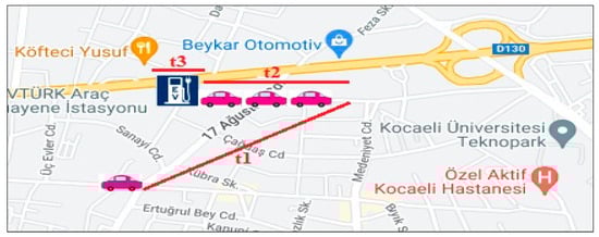
Figure 1.
Organization of the study.
Deep learning approaches with time series, recognized in the literature for their superior prediction, have garnered considerable attention in electric vehicles and charging stations. But predicting the charging demand and battery charge estimation has been limited to EV charging station positioning. This study aimed to estimate the charging process time, which is unprecedented in previous studies.
2. Data Set
The high use of missing or inaccurate data in the studies may lead to poor forecasting results. To improve forecast performance, real data must be used, and data gaps must be filled carefully. In this study, the researchers tried to use real data as much as possible. However, electric vehicles are a new technology that does not have a very long history. For this reason, there may be problems with the data. In the study, two groups of data sets, charging stations and EVs, are needed for charging time calculation. Among these data sets, all real data were used for charging stations. The data for EVs belong to recent years and are only shared as a piece of information. For this reason, while preparing the data set for EVs, the battery capacities of the vehicles used in the market were considered to obtain healthy results.
For the data set used to test the proposed LSTM, GRU, Prophet, and ARIMA models and to decide on the most appropriate model for charging time estimation, the actual locations of 45 charging stations in Kocaeli province in Turkey were used. Using Google Maps, the “My Map” feature shows the locations of 45 charging stations in the region, as shown on the map in Figure 2. Data belonging to approximately 100 electric vehicles were used to ensure the utilization of the charging stations. These vehicles were randomly distributed on the map, and location information was obtained.
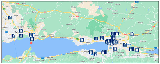
Figure 2.
Location of 45 charging stations in Kocaeli on Google Maps.
While preparing the data set of the charging stations in the study, a total of 180 data points were added, including the name of each charging station, power information, the number of vehicles that can be charged at the same time, and the location of the charging station with latitude and longitude degrees. Then, a total of 312 data points were added, including the names of 104 EVs and their battery capacities and battery occupancy rates.
2.1. Data Sources
In the study, the data are focused on two sources: EVs and EV charging stations. The quantity of information on these data sources is shown in Table 1.

Table 1.
Data sources.
The power of the 16 DC charging stations in the table is 180 kW, 120 kW, and 50 kW. The power of the 17 AC charging stations in the table is 22 kW and 50 kW. For 12 charging stations, only location information is available for remote access, and no other information is shared for the driver to access before arriving at the charging station. The power values of these charging stations were filled with the most frequently occurring value in the data set. The battery values of 104 vehicles in the table are 100 kW, 95 kW, 90 kW, 80 kW, 75 kW, and 50 kW. However, the battery charge rate of each vehicle was selected at different values, and values between 21 and 50% were given. Repetitive battery charge rates were detected and changed. Figure 3 shows visualizations of data distributions. Figure 3 shows two graphs: the power distribution of charging stations and the EV battery capacity distribution.
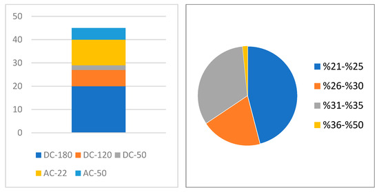
Figure 3.
Visualization of data distributions.
2.2. Data Preprocessing
After the data set was prepared, the study aimed to evaluate all possibilities in order to decide on the most appropriate model for time calculation. For this reason, the charging time of all vehicles was calculated at all stations where power information was accessed from the charging stations used in the study. Here, Equation (1) as follows is used for charging time.
To calculate the time in the equation at the charging stations, 494,394 rows and 7 columns of data were processed. The training time of the LSTM model was 1 h and 57 min, the training time of the GRU model was 1 h and 40 min, the training time of the ARIMA model was 6 h and 69 min, and the training time of the Prophet model was 5 h and 10 min. Considering the model training times, it is seen that the training of LSTM and GRU is completed faster. The reason for this is that ARIMA and Prophet show poorer performance as the number of variables increases, whereas LSTM and GRU are completed faster. When LSTM and GRU are compared, LSTM has more parameters, which can result in slightly slower training times compared to GRU, especially on larger data sets. With fewer parameters, GRU may have faster training times, making it more efficient for larger data sets.
Since it is a time series, the rows of the data set to be used in the model were timestamped. Accordingly, a column named “Time” was created, and the data type was set as “datetime”. For the transition from one row to another, the difference between them corresponds to 1 min.
The correlation between the predicted and actual values is presented in Figure 4. It shows an overview of the forecasting results and real values achieved by all models. A correlation coefficient (R2) value of 1 indicates a perfect positive correlation. In Figure 4, LSTM and GRU showed the most perfect correlation with the value closest to 1. Each of the predicted results and actual values obtained by all models are marked and form the blue areas.
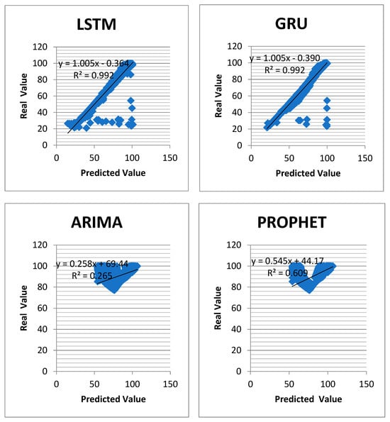
Figure 4.
Correlation between the predicted and the actual value using different models.
3. Materials and Methods
Artificial neural networks are very successful in forecasting using current data, while time series are very successful in predicting the future by analyzing accurate data from the past. In this study, deep learning LSTM, GRU, ARIMA, and Prophet time series models of artificial neural networks were used.
Figure 5 summarizes the flowchart of the study. The flowchart is divided into three groups. First, the study started with the collection of real-life data. In the second phase, LSTM, Prophet, GRU, and ARIMA models were created. The data collected in the first phase were divided and used in the training and testing phases of the models. Then, with the data allocated for training, the training of each model was completed, and prediction values were obtained. In the last stage, R2, MSE, MAE, and DTW metrics were used to decide which model is more accurate by using the prediction and test values obtained.
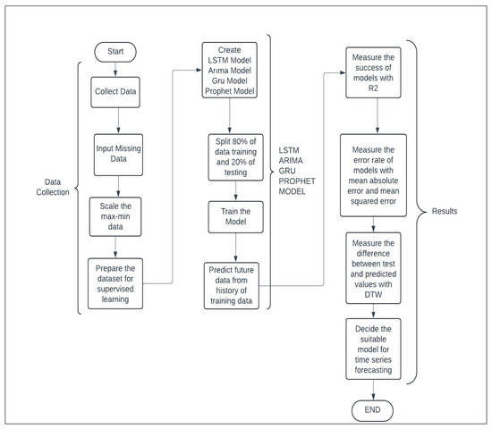
Figure 5.
Flowchart.
For the creation of the time series to be used in model training, the
| generate_charging_time_series |
- function is used to obtain a time series, and the vehicle charge is tracked in minute increments. Each vehicle and charging station’s information was also included in the model, and vehicle and station information was used as an identifier. Information about the station and vehicles was also included in the data so that it could be used as an identifier if needed in the later stages of the project.
During the development of the models with Python, libraries were created for this purpose. The data set obtained was converted into a format suitable for the models. The libraries prepared for LSTM and ARIMA were imported as follows:
| from statsmodels.tsa.arima.model import ARIMA from prophet import Prophet from keras.layers import LSTM from keras.layers import GRU |
Of the available data, 80% are reserved for training, and the remaining 20% are reserved for evaluating model performance. The columns in the data set were filtered according to the information required by the models. After filtering, the models were trained with the following codes.
3.1. LSTM
LSTM is an architecture of the RNN used in artificial intelligence and deep learning. LSTM is particularly good at multivariate classification, processing, and prediction using time series data. An LSTM network has the following characteristics that distinguish it from a regular neuron in a recurrent neural network: it has control over deciding when the input enters the neuron, control over deciding when it remembers what was calculated in the previous time step, and control over deciding when the output moves on to the next timestamp. LSTM’s advantage is that it decides all this based on the current input itself.
The LSTM is a set of nodes of a recurrent neural network and has three gates, the input, output, and forget gates, which decide which node the signals go to. Figure 6 shows the block model of the LSTM. Here, f(t) is the forget gate, i(t) is the input gate, and o(t) is the output gate.
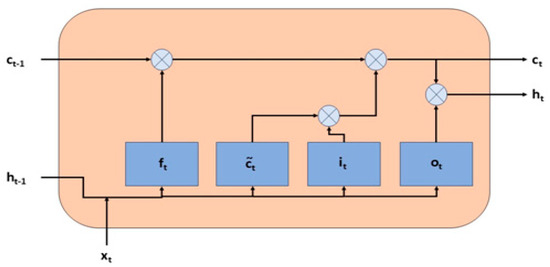
Figure 6.
LSTM block model.
The input gate decides which of the data points is important and will pass through the model. The input gate consists of two layers: the sigmoid (σ) layer, which decides which values to update, and the tanh layer, which generates new candidate data. The equation for the output i(t) of the input gate is expressed by the formula in Equation (2).
The equation Ĉ(t) of the tanh layer representing the new data is expressed by the formula in Equation (3).
The forget gate decides which of the previous information to keep. The output function f(t) of the forget gate is expressed by the formula in Equation (4).
In the input gate, i(t) and Ĉt are combined and updated to determine which data will pass through the model. Then, at each step, the previous cell state Ct−1 is combined with the forget gate to decide which information to pass to the next step. Finally, this forget gate and the input gate are combined to create a new memory. This process is expressed by the formula in Equation (5).
The output gate enables the LSTM model to provide output. The output gate o(t) is expressed by the formula in Equation (6).
It is desirable to limit the results obtained to values between −1 and 1. Therefore, the memory state h(t) is obtained by passing Ct obtained in Equation (7) through the tanh function.
In the experiments, W represents the weight matrix, b the bias term, x(t) the current input, and ht−1 the previous memory state.
3.2. GRU
GRU is an improvement over the traditional recurrent neural network (RNN), addressing the vanishing gradient problem. GRU can selectively retain or discard information from the past, making it better at capturing long-term dependencies than a simple RNN. It is an advanced version of an RNN that can selectively remember or forget information.
The GRU model is very similar to LSTM. As in LSTM, gates are used for information flow, but it has a newer and simpler architecture than LSTM. The advantage of this simpler architecture is that it is faster to train. Unlike LSTM, GRU does not have three gates but two gates, reset and update gates. Through these gates, it is decided which information to transmit to the output. Figure 7 shows the block diagram of the GRU model. Here, r(t) is the reset gate, and z(t) is the update gate.
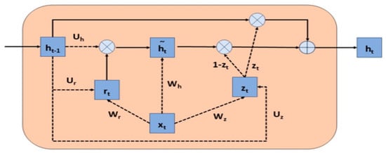
Figure 7.
GRU block model.
The update gate is obtained by combining the forget and input gates in the LSTM. The update gate decides how much of the past information from the previous time steps is transferred to the future. The update gate is obtained by multiplying the input vector x(t) by the weight vector of the hidden state vector h(t−1) of the previous step h(t−1) and then combining them by applying a sigmoid layer defined by the formula in Equation (8).
The reset gate decides how much of the information passing through the model is forgotten. The calculation process for the reset gate is the same as for the update gate but with different weight values. The reset gate is expressed by Equation (9).
Equations (5) and (6) are used to see how the reset and update gates affect the output. The preparation of new memory content using the reset gate to store information about the past is shown in Equation (10) with ĥt.
The update gate, which controls the past information from one step before and the new information from the current memory ht, is shown in Equation (11).
In the experiments, W represents the weight matrix, b the bias term, x(t) the current input, and ht−1 the hidden state.
3.3. ARIMA
ARIMA is a combination of autoregressive modeling (AR) and moving average modeling approaches for forecasting time series data. The AR model forecasts future values of the time series based on past data. The MA model forecasts future values based on averages of past data over a specific time period and uses the average of the error terms. The ARIMA model block diagram is shown in Figure 8.
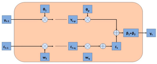
Figure 8.
ARIMA block model.
Combining the AR and MA equations, the ARIMA model is expressed by Equation (12).
Yt and represent estimated values, represents the AR model coefficient, represents the MA model coefficient, and ß represents the series mean. The p-value indicates how much historical data to look at from the end. The q value indicates how many error terms are averaged from the end.
3.4. PROPHET
Prophet is a time series model that forecasts daily, weekly, monthly, and yearly data. It forecasts very fast by managing missing and outlier data values very well. The block diagram of the Prophet model is shown in Figure 9.
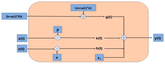
Figure 9.
Prophet block model.
The Prophet model is expressed by Equation (13).
In the Prophet equation, g(t) is the trend factor modeling non-periodic long-term changes and is expressed by Equation (14).
s(t) in the Prophet equation is the seasonality component that models periodic changes and is expressed by Equation (15).
In the Prophet equation, h(t) is the vacation component that significantly affects the time series and is expressed by Equation (16).
3.5. Evaluation Criteria
In the third stage of the flowchart in Figure 3, the predictions made by the models are compared with the test data. In the study, four evaluation metrics were preferred for the performance evaluation of each of the models. Three of them are the more common MSE (Mean Squared Error), MAE (Mean Absolute Error), and R2 (R-squared). The less common DTW (Dynamic Time Warping) was used as the fourth evaluation metric. The equations described below were used to calculate these metrics.
The MSE metric is an error metric that gives the mean square of the difference between the predicted and actual values. The lowest MSE indicates a superior model. The MSE metric is expressed by Equation (17).
The MAE metric is an error metric that gives the mean absolute value of the difference between the predicted and actual values. The lowest MAE indicates a superior model. The MAE metric is expressed by Equation (18).
The R2 metric is a value between 0 and 1 that indicates how well the model predicts the outcome. If the result is 0, the model fails to predict it; if it is between 0 and 1, it predicts it, albeit imperfectly, but if it is 1, it predicts it perfectly. The R2 metric is expressed by Equation (19).
The DTW metric is a distance metric that finds the difference between similar items in a time series by matching them. Therefore, it measures the distance between the predicted and test values and considers the one with the smallest distance to be successful. The DTW metric is expressed by Equation (20).
In the equations of the metrics, ý represents prediction values, y represents test values, and n represents sample size.
4. Findings and Analysis
The training processes of the models in this study were completed in Python 3.12.2 using Pandas 2.2.2, Numpy 2.1.2, Statsmodel 0.14.4, Sklearn 1.5.2, Flask 3.0.3, and Keras 2.4.3 frameworks.
The study applied training hyperparameters that directly optimize the training process of the manually tuned model. These parameters are defined before the model training starts and are not changed once the model training starts.
The optimization algorithm used for the LSTM and GRU model is Adam, and the learning rate is set to 0.001. To improve the training efficiency, the training methodology is adopted where each iteration consists of 16 data sets, and the number of iterations is set to 50. For each model, data analysis was performed considering 10 charging process times corresponding to 10 min.
The hyperparameter values in the study are general values and are widely preferred in the literature. The hyperparameters used for LSTM and GRU, which give better results in the study, are shown in Table 2.
Table 2.
LSTM and GRU model hyperparameters.
For the first-order AR model and the ARIMA model called second-order MA, the hyperparameters p, d, and q are set to (1,0,2).
For Prophet, the interval with the parameter is set to 0.95 for a 95% prediction interval.
After the training processes of LSTM, GRU, Prophet, and ARIMA models were completed, success checks were made, and their scores were recorded and compared. Each method was repeated five times with the same parameters. The mean result was obtained by averaging these five results. The results of the first five steps of each model over the prediction and test values are shown in Table 3. Score calculations were made based on these values. Table 3 shows the test and prediction values.
Table 3.
Test and prediction values of models.
Based on the values in the table, R2, MAE, MSE, and DTW metrics were used to evaluate the performance of the models. Firstly, the R2 score was analyzed. Figure (a) shows the results of each model for the R2 metric. Since R2 is a success metric, the model with a value of 1 or the closest model predicts values better. In Figure 10a, the results for ARIMA and Prophet are quite low. The reason for this is that these two models are not good at analyzing different probability cases. In the study, the estimation of the charging time of each vehicle for each charging station caused these two models to give poor results. If each vehicle had been charged at one charging station, these models would have provided higher scores. LSTM and GRU provided the highest R2 scores. This is an expected result. This is expected as LSTM and GRU enable flexibility in managing multiple situations.
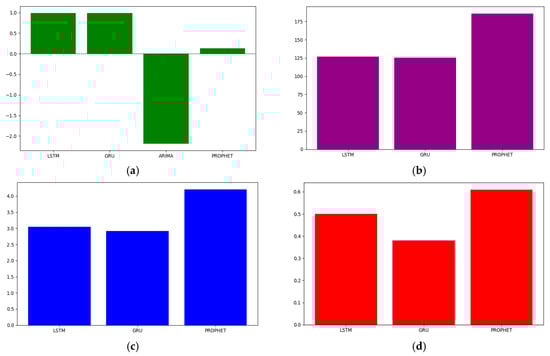
Figure 10.
R2,DTW, MSE, and MAE values of the models. (a) R2 values of the models. (b) DTW values of the models. (c) MSE values of models. (d) MAE values of the models.
The R2 scores show that ARIMA is clearly not successful in calculating the charging time. The scores of the other models, especially LSTM and GRU, are very close to each other. Another metric where the scores are very close to each other is DTW. In DTW and error metrics, unlike R2, the smaller the score, the more successful the model. The figure shows the scores of the DTW metric. ARIMA scores are not included here. This is because the values of the ARIMA model are too high, which negatively affects the accuracy of evaluating the results of other models. When the scores of the DTW metric are analyzed in Figure 10b, the scores of the LSTM and GRU models are very close to each other. Prophet was more unsuccessful compared to these models.
Although the R2 and DTW metrics did not determine the exact result, they showed that Prophet and ARIMA were less successful. In particular, the LSTM and GRU models were evaluated based on the number of errors made due to the close scores. Figure 10c shows the scores of the MSE metric. The GRU model has a lower error rate.
Figure 10d shows the scores of the MAE metric. It is more evident from the MSE metric scores that the GRU model has a lower error rate.
It has been determined that GRU is the most successful model in the time calculation of electric vehicle charging processes.
For drivers who want to use the 45 charging stations in Kocaeli province, the sum of the arrival to the charging station from the point where they are located, the charging time of the vehicles if there are vehicles in the queue, and the charging time of the vehicle when it is their turn will be calculated with the GRU model.
An interface has been designed that can be used as a simulation for the GRU model to estimate time. An example of this interface is shown as a tool on the application. The interface will ask the user to enter some data and generate predictions using the data provided. First, as shown in Figure 11, the driver’s location is requested to be marked on the map. In addition, the vehicle’s battery capacity, current occupancy rate, and the same information are requested separately for the vehicle or vehicles waiting in the queue.
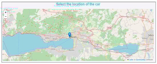
Figure 11.
Location of the driver (time to reach the charging station was measured based on the traffic density at 23.11.2024 21.28).
First, as shown in Figure 12, the driver is shown their current location, the battery capacity of the vehicle, and how much of this capacity is full. The battery of the selected vehicle is 95 kWh, and the battery occupancy rate is 30%.
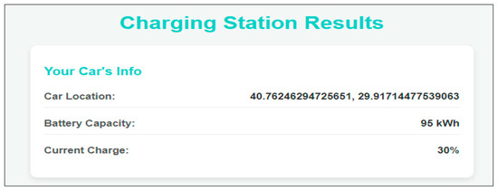
Figure 12.
Vehicle information.
When the vehicle location is marked on the map in Figure 11, the driver is shown the name and location of the nearest charging station, the power of the charging station, and the number of vehicles that can be charged at the same time, as shown in Figure 13.
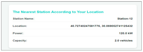
Figure 13.
Information on the nearest charging station to the vehicle.
The distance from the driver’s location to the nearest charging station and the arrival time, depending on the current traffic density, is shown in Figure 14. The distance of the vehicle marked on the map to the nearest charging station, Station-12, is approximately 1.4 km. On 23.11.2024 at 21.28, the arrival time to Station-12 is approximately 13 min, depending on the traffic density at the time the vehicle was marked on the map.
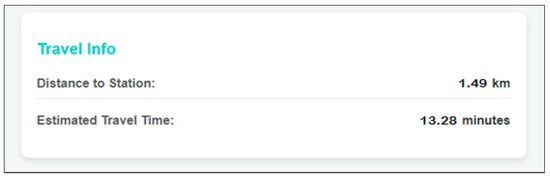
Figure 14.
Information on the arrival process of the vehicle at the station.
At first, the information of the two vehicles in the queue was added to the interface as 80 kWh battery capacity and 20% occupancy rate, as well as 50 kWh battery capacity and 47% occupancy rate. Based on these occupancy rates, the charging time of these vehicles at Station-12 with 120 kW power is approximately 75 min, as shown in Figure 15. This is the waiting time of the vehicle in the queue. When it is the turn of the vehicle whose location is marked on the map, the charging time of the 95 kWh vehicle with a 30% occupancy rate is approximately 55 min at Station-12.
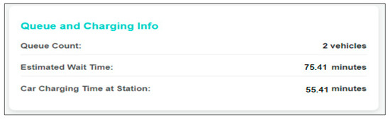
Figure 15.
Information about the waiting time and charging time of the vehicle at the station.
When it was the driver’s turn, the charging time at Station-12 was calculated to be approximately 55 min. The change in charging time and occupancy rate during this charging process is shown in Figure 16.
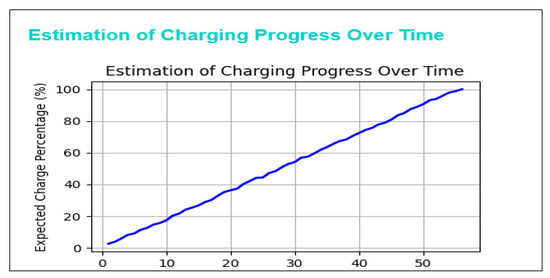
Figure 16.
Change in charging time–battery occupancy rate.
In the study, time calculations on an example were calculated using the GRU model, which gives the most accurate result. The process of arriving at the nearest charging station using the location of a vehicle marked on the map application, waiting in the queue, and charging will take approximately 138 min. Considering this time, it is up to the driver to choose Station-12 or to head to another station. The driver can learn the same time estimation if he wants to use another charging station.
A second example is shown in Figure 17.
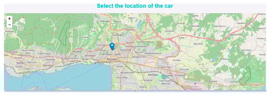
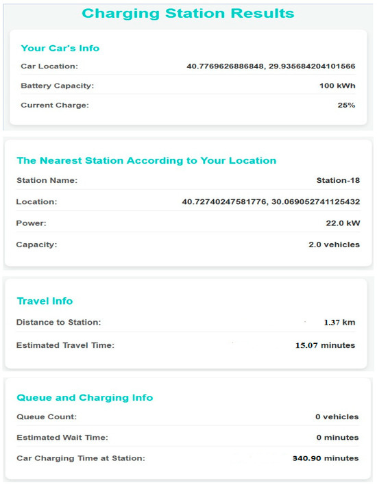
Figure 17.
Estimated arrival and charging times at the GRU model charging station.
In Figure 17, the driver’s location and the time to reach the charging station were measured according to the traffic density as of 16.50 on 23 March 2025.
5. Conclusions
In this study, an application that can be integrated into the vehicle is proposed to increase the sustainability of the transportation sector by ensuring the adoption of EVs. In addition, with the use of the application that can be integrated into the vehicle, effective use of charging resources might be ensured. With the EV and charging station data considered in the study, each of the various deep learning methods was examined in detail to calculate the charging process and the waiting time in the queue before the charging station, and the model that gave the most accurate result was determined. After the training processes of LSTM, GRU, Prophet, and ARIMA models were completed, the GRU model produced the most accurate result when compared with R2 (0.99), MSE (2.92), MAE (0.38), and DTW (125.5) metrics. If it were not possible to choose the metrics preferred in the evaluation of the models, the response time of the models would be taken into consideration, and the model with the fastest response would be preferred. When the system response time is evaluated for the practical application effect of the system, each model completed this in less than 1 s. However, the shortest time belongs to the GRU model with a difference of milliseconds.
In the application shown with the interface in the study, some data were manually entered into the system. However, when this application is integrated into electric vehicles, vehicle information will be sent to the automatic application without the need to enter the data manually.
It has been verified that the GRU model provides better prediction accuracy and minimum error values in future studies to predict the charging time calculation for EVs.
In future studies, it is aimed to add probabilistic optimization methods and statistical analysis of existing data together with deep learning methods in studies on electric vehicles and charging stations. In the study, an application was made in a certain region in Kocaeli province. It can be applied to the entire region when all charging stations in the region and the data belonging to these stations can be accessed.
Author Contributions
A.T.Y.: conceptualization, methodology, software, writing—original draft, data curation. N.A.: supervision, project administration. T.E.: writing—review and editing, methodology. All authors have read and agreed to the published version of the manuscript.
Funding
This research received no external funding.
Data Availability Statement
The original contributions presented in the study are included in the article, further inquiries can be directed to the corresponding author.
Acknowledgments
We are grateful to all those who have helped us during the research process.
Conflicts of Interest
The authors declare no conflicts of interest.
Abbreviations
The following abbreviations are used in this manuscript:
| ARIMA | Autoregressive Integrated Moving Average |
| ACNN | A Convolutional Neural Network |
| DTW | Dynamic Time Warping |
| EV | Electric Vehicle |
| GRU | Gated Recurrent Unit |
| LSTM | Long Short-Term Memory |
| MAE | Mean Absolute Error |
| MSE | Mean Squared Error |
| R2 | R-squared |
| RNN | Recurrent Neural Network |
| SARIMA | Seasonal Autoregressive Integrated Moving Average |
References
- Mehlig, D.; Staffell, I.; Stettler, M.; ApSimon, H. Accelerating Electric Vehicle Uptake Favours Greenhouse Gas Over Air Pollutant Emissions. Transport. Res. Part D Transp. Environ. 2023, 124, 212543. [Google Scholar] [CrossRef]
- Alanazi, F. Electric vehicles: Benefits, Challenges, and Potential Solutions for Widespread Adaptation. Appl. Sci. 2023, 13, 6016. [Google Scholar] [CrossRef]
- Martínez-Gómez, J.; Espinoza, V.S. Challenges and Opportunities for Electric Vehicle Charging Stations in Latin America. World Elect. Veh. J. 2024, 15, 583. [Google Scholar] [CrossRef]
- Metais, M.O.; Jouini, O.; Perez, Y.; Berrada, J.; Suomalainen, E. Too much or not Enough? Planning Electric Vehicle Charging Infrastructure: A Review of Modeling Options. Renew. Sustain. Energy Rev. 2022, 153, 111719. [Google Scholar] [CrossRef]
- Huang, Y.; Kockelman, K.M. Electric vehicle charging station locations: Elastic demand, station congestion, and network equilibrium. Transp. Res. Part D Transp. Environ. 2020, 78, 102179. [Google Scholar] [CrossRef]
- Abdullah, D. Hibrid, Tam Elektrikli ve Yakit Hücreli Araçlar Trendi ve Emniyet Yükümlülüklerinin Değerlendirilmesi. İstanbul Ticaret Üniversitesi Fen Bilim. Derg. 2022, 21, 136–155. [Google Scholar]
- Dvořáček, L.; Horák, M.; Valentová, M.; Knápek, J. Optimization of Electric Vehicle Charging Points Based on Efficient Use of Chargers and Providing Private Charging Spaces. Energies 2020, 13, 6750. [Google Scholar] [CrossRef]
- Pan, L.; Yao, E.; Yang, Y.; Zhang, R. A Location Model for Electric Vehicle (EV) Public Charging Stations Based on Drivers’ Existing Activities. Sustain. Cities Soc. 2020, 59, 102192. [Google Scholar] [CrossRef]
- Mastoi, M.S.; Zhuang, S.; Munir, H.M.; Haris, M.; Hassan, M.; Usman, M.; Bukhari, S.S.H.; Ro, J. An In-Depth Analysis of Electric Vehicle Charging Station Infrastructure, Policy Implications, and Future Trends. Energy Rep. 2022, 8, 11504–11529. [Google Scholar] [CrossRef]
- Vaidya, B.; Mouftah, H.T. Smart Electric Vehicle Charging Management for Smart Cities. IET Smart Cities 2020, 2, 4–13. [Google Scholar] [CrossRef]
- Chawrasia, S.K.; Hembram, D.; Bose, D. Design of Solar Battery Swapping Station for EV Using LSTM-Assisted Solar Power Forecasting. Microsyst. Technol. 2024, 30, 1087–1098. [Google Scholar] [CrossRef]
- Güldorum, H.C.; Şengör, İ.; Erdinç, O. Management Strategy for V2X Equipped EV Parking loT Considering Uncertainties with LSTM Model. Elect. Power Syst. Res. 2022, 212, 108248. [Google Scholar] [CrossRef]
- Hafeez, A.; Alammari, R.; Iqbal, A. Utilization of EV Charging Station in Demand Side Management Using Deep Learning Method. IEEE Access 2023, 11, 8747–8760. [Google Scholar] [CrossRef]
- Khezri, R.; Razmi, P.; Mahmoudi, A.; Bidram, A.; Khooban, M.H. Machine Learning-Based Sizing of a Renewable-Battery System for Grid-Connected Homes with Fast-Charging Electric Vehicle. IEEE Trans. Sustain. Energy 2023, 14, 837–848. [Google Scholar] [CrossRef]
- Shaza, H.; Mansour, S.M.; Azzam, H.M.; Hasanien, M.T.; Abdulaziz, A.; Francisco, J. Deep reinforcement learning-based plug-in electric vehicle charging/discharging scheduling in a home energy management system. Energy 2025, 316, 134420. [Google Scholar]
- Terala, P.K.; Ogundana, A.S.; Foo, S.Y.; Amarasinghe, M.Y.; Zang, H. State of Charge Estimation of Lithium-Ion Batteries Using Stacked Encoder-Decoder Bi-Directional LSTM for EV and HEV Application. Micromachines 2022, 13, 1397. [Google Scholar] [CrossRef]
- Hossain Lipu, M.S.; Shaheer, A.; Miah, M.S.; Meraj, S.T.; Hasan, K.; Shihavuddin, A.S.M.; Hannan, M.A.; Kashem, M.; Muttaqi, A.H. Deep Learning Enabled State of Charge, State of Health and Remaining Useful Life Estimation for Smart Battery Management System: Methods, Implementations, Issues and Prospects. J. Energy Storage 2022, 55, 105752. [Google Scholar] [CrossRef]
- Tian, J.; Chen, C.; Shen, W.; Sun, W.; Xiong, R. Deep Learning Framework for Lithium-Ion Battery State of Charge Estimation: Recent Advances and Future Perspectives. Energy Storage Mater. 2023, 61, 102883. [Google Scholar] [CrossRef]
- Zafar, M.H.; Mansoor, M.; Abou Houran, M.; Mujeeb Khan, N.; Khan, K.; Moosavi, S.Y.R.; Sanfilippo, F. Hybrid Deep Learning Model for Efficient State of Charge Estimation of Li-ion Batteries in Electric Vehicles. Energy 2023, 282, 128317. [Google Scholar] [CrossRef]
- Hong, S.; Hwang, H.; Kim, D.; Cui, S.; Joe, I. Real Driving Cycle-Based State of Charge Prediction for EV Batteries Using Deep Learning Methods. Appl. Sci. 2021, 11, 11285. [Google Scholar] [CrossRef]
- Shi, D.; Zhao, J.; Wang, Z.; Zhao, H.; Eze, C.; Wang, J.; Lian, Y.; Burke, A.F. Cloud –Based Deep Learning for Co-Estimation of Battery State of Charge and State of Health. Energies 2023, 16, 3855. [Google Scholar] [CrossRef]
- Sulaiman, M.H.; Mustaffa, Z.; Razali, S.; Daud, M.R. Advancing Battery State of Charge Estimation in Electric Vehicles Through Deep Learning: A Comprehensive Study Using Real-World Driving Data. Clean. Energy Syst. 2024, 8, 100131. [Google Scholar] [CrossRef]
- Lipu, H.; Karim, M.S.; Ansari, T.F.; Miah, S.; Rahman, M.S.; Meraj, M.S.; Elavarasan, S.T.; Vijayaraghavan, R.R. Intelligent SOX Estimation for Automotive Battery Management Systems: State-of-the-Art Deep Learning Approaches, Open Issues, and Future Research Opportunities. Energies 2023, 16, 23. [Google Scholar] [CrossRef]
- Liu, Y.; He, Y.; Bian, H.; Guo, W.; Zhang, X. A Review of Lithium-Ion Battery State of Charge Estimation Based on Deep Learning: Directions for Improvement and Future Trends. J. Energy Storage 2022, 52, 104664. [Google Scholar] [CrossRef]
- Yi, Z.; Liu, X.C.; Wei, R.; Chen, X.; Dai, J. Learning Electric Vehicle Driver Range Anxiety with an Initial State of Charge-Oriented Gradient Boosting Approach. J. Intell. Transp. Syst. 2021, 26, 690–703. [Google Scholar] [CrossRef]
- Wang, S.; Zhuge, C.; Shao, C.; Wang, P.; Yang, X.; Wang, S. Short-Term Electric Vehicle Charging Demand Prediction: A Deep Learning Approach. Appl. Energy 2023, 340, 121032. [Google Scholar] [CrossRef]
- Van Kriekinge, G.; De Cauwer, C.; Sapountzoglou, N.; Coosemans, T.; Messagie, M. Day-Ahead Forecast of Electric Vehicle Charging Demand with Deep Neural Networks. World Electr. Veh. J. 2021, 12, 178. [Google Scholar] [CrossRef]
- Zhang, X.; Chan, K.W.; Li, H.; Wang, H.; Qiu, J.; Wang, G. Deep-Learning-Based Probabilistic Forecasting of Electric Vehicle Charging Load with a Novel Queuing Model. IEEE Trans. Cybern. 2021, 51, 3157–3170. [Google Scholar] [CrossRef]
- Boulakhbar, M.; Farag, M.; Benabdelaziz, K.; Kousksou, T.; Zazi, M. A Deep Learning Approach for Prediction of Electrical Vehicle Charging Stations Power Demand in Regulated Electricity Markets: The Case of Morocco. Clean. Energy Syst. 2022, 3, 100039. [Google Scholar] [CrossRef]
- Eddine, M.D.; Shen, Y. A Deep Learning Based Approach for Predicting the Demand of Electric Vehicle Charge. J. Supercomput. 2022, 78, 14072–14095. [Google Scholar] [CrossRef]
- Lu, F.; Jian, L.; Zhang, Y.; Liu, H.; Zheng, S.; Li, Y.; Hong, M. Ultra-Short-Term Prediction of EV Aggregator’s Demond Response Flexibility Using ARIMA, Gaussian-ARIMA, LSTM and Gaussian-LSTM. In Proceedings of the 2021 3rd International Academic Exchange Conference on Science and Technology Innovation, Guangzhou, China, 10–12 December 2021. [Google Scholar]
- Chang, M.; Bae, S.; Cha, G.; Yoo, J. Aggregated Electric Vehicle Fast-Charging Power Demand Analysis and Forecast Based on LSTM Neural Network. Sustainability 2021, 13, 13783. [Google Scholar] [CrossRef]
- Koohfar, S.; Woldemariam, W.; Kumar, A. Performance Comparison of Deep Learning Approaches in Predicting EV Charging Demand. Sustainability 2023, 15, 4258. [Google Scholar] [CrossRef]
- Akshay, K.C.; Grace, G.H.; Gunasekaran, K.; Samikannu, R. Power Consumption Prediction for Electric Vehicle Charging Stations and Forecasting Income. Sci. Rep. 2024, 14, 6497. [Google Scholar] [CrossRef]
- Alansarlı, M.; Al-Sumaiti, A.S.; Abughali, A. Optimal Placement of Electric Vehicle Charging Infrasctructures Utilizing Deep Learning. IET Intell. Transp. Syst. 2024, 18, 1529–1544. [Google Scholar] [CrossRef]
- Gulbahar, I.T.; Sütçü, M.; Almomany, A.; İbrahim, B.S.K.K. Optimizing Electric Vehicle Charging Station Location on Highways: A Decision Model for Meeting Intercity Travel Demand. Sustainability 2023, 15, 16716. [Google Scholar] [CrossRef]
- Aldossary, M.; Alharbi, H.A.; Ayub, N. Optimizing Electric Vehicle (EV) Charging with Integrated Renewable Energy Sources: A Cloud-Based Forecasting Approach for Eco-Sustainability. Mathematics 2024, 12, 2627. [Google Scholar] [CrossRef]
- Zhang, H.; Li, Z.; Xue, Y.; Chang, X.; Su, J.; Wang, P. A Stochastic Bi-Level Optimal Allocation Approach of Intelligent Buildings Considering Energy Storage Sharing Services. IEEE Trans. Consum. Electron. 2024, 70, 5142–5153. [Google Scholar] [CrossRef]
- Shengyou, W.; Yuan, L.; Chunfu, S.; Pinxi, W.; Aixi, W.; Chengxiang, Z. An adaptive spatio-temporal graph recurrent network for short-term electric vehicle charging demand prediction. Appl. Energy 2025, 383, 125320. [Google Scholar]
- Xu, X.; Wu, J.; Lu, Y.; Liu, Y.; Zhao, H. A spatio-temporal prediction approach for charging load of clustered electric vehicles in dynamic traffic flow environment of highway. Sustain. Energy Grids Netw. 2024, 40, 101593. [Google Scholar] [CrossRef]
- Selvam, P.A.; Subramani, J. Optimized Deep Reinforcement Learning for Smart Charging Scheduling of Plug-in Electric Vehicles. Electr. Power Compon. Syst. 2023, 51, 2085–2097. [Google Scholar] [CrossRef]
- Ma, J.; Roncoli, C.; Ren, G.; Yang, Y.; Wang, S.; Yu, J.; Wang, B. An integrated framework for fully sampled vehicle trajectory reconstruction using a fused dataset. Transp. A Transp. Sci. 2025, 21, 1–30. [Google Scholar] [CrossRef]
- Pourvaziri, H.; Sarhadi, H.; Azad, N.; Afshari, H.; Taghavi, M. Planning of electric vehicle charging stations: An integrated deep learning and queueing theory approach. Transp. Res. Part E Logist. Transp. Rev. 2024, 186, 103568. [Google Scholar] [CrossRef]
- Feng, R.; Hua, Z.; Yu, J.; Zhao, Z.; Dan, Y.; Zhai, H.; Shu, X. A comparative investigation on the energy flow of pure battery electric vehicle under different driving conditions. Appl. Therm. Eng. 2025, 269, 126035. [Google Scholar] [CrossRef]
Disclaimer/Publisher’s Note: The statements, opinions and data contained in all publications are solely those of the individual author(s) and contributor(s) and not of MDPI and/or the editor(s). MDPI and/or the editor(s) disclaim responsibility for any injury to people or property resulting from any ideas, methods, instructions or products referred to in the content. |
© 2025 by the authors. Licensee MDPI, Basel, Switzerland. This article is an open access article distributed under the terms and conditions of the Creative Commons Attribution (CC BY) license (https://creativecommons.org/licenses/by/4.0/).