Novel Real-Time Power System Scheduling Based on Behavioral Cloning of a Grid Expert Strategy with Integrated Graph Neural Networks

Abstract

Amidst the large-scale integration of renewable energy, power grid operations are increasingly characterized by higher levels of uncertainty, challenging the system’s safety and stability. Traditional model-driven dispatch methods are computationally intensive, and recent Reinforcement Learning (RL) techniques struggle with slow training times due to high-dimensional state spaces, while the inability to fully utilize the system’s topology information affects scheduling accuracy. This paper introduces a novel Behavioral Cloning of Grid Expert Strategy with Integrated Graph Neural Networks (GES-GNNBC) method for efficient and highly accurate real-time dispatch. The approach integrates grid expert strategies with graph theory-based modeling and Behavioral Cloning (BC), capturing the topological information of the power grid through Graph Neural Networks (GNN) to improve scheduling accuracy. Tested on a modified IEEE 33-bus model rich in renewable sources, GES-GNNBC outperforms both traditional and RL methods in stability and efficiency of computing optimization schemes and power balance strategies, markedly improving dispatch decision-making speed and effectiveness.

1. Introduction

In recent years, with the rapid development of renewable energy resources, a new type of electric power system characterized by cleanliness, low carbon emissions, intelligent friendliness, and interactive openness has gradually taken shape. Against the backdrop of this new electric power system, the intermittency, volatility, and uncertainty of a high proportion of renewable energy sources have led to the “trilemma” of energy security, economy, and sustainability. Navigating this predicament has become a significant challenge for grid dispatch departments [1]. Grid dispatching strategies, according to their temporal scale, can be divided into day-ahead scheduling, intra-day scheduling, and real-time scheduling. Among these, real-time scheduling, which demands the highest computational timeliness, further corrects the outcomes of day-ahead and intra-day scheduling based on accurate ultra-short-term forecasts of renewable energy sources and loads. However, the real-time dispatch has limited capabilities for mobilizing the flexible resources of units within a short timeframe [2], and it is challenging to precisely achieve power balance and meet the N-1 operating requirements [3], especially in scenarios with a high proportion of renewable energy. Therefore, designing a secure and efficient real-time dispatch method for modern power systems is of crucial importance.

Traditional power grid scheduling primarily employs model-driven approaches, constructing power system models that account for typical operational scenarios. These models are utilized to analyze and optimize grid operation strategies against various system constraints based on the model [4,5,6,7,8]: scheduling methods based on grid expert strategies [4] typically utilize models incorporating a limited number of grid forecast scenarios for offline fault analysis, identifying system vulnerabilities, and then formulating scheduling plans based on dispatchers’ personal experience [5]. However, grid expert strategy methods struggle to promptly address real-time safety issues in scenarios with a high proportion of renewable energy sources and are insufficiently adaptable; moreover, traditional methods have a low level of intelligence, with decision-making being prone to human error [5]. Scheduling methods based on mathematical optimization algorithms, with solving techniques primarily including robust optimization [6], stochastic programming [7], and chance-constrained programming [8]. Reference [6] utilizes robust optimization to establish a grid scheduling model considering the uncertainty of wind power output, yet this method generates overly conservative scheduling decisions due to its strict adherence to operational safety constraints during the solution process, failing to fully exploit the system’s potential to absorb renewable energy sources. Reference [7] applies stochastic programming to transform a grid scheduling model with wind power output uncertainty into a deterministic scheduling model for a solution, but this method faces challenges due to the uncertainty of renewable energy outputs and the large scale of probabilistic modeling. Reference [8] describes wind power output uncertainty using a Gaussian mixture model and proposes a chance-constrained programming scheduling method, converting hard constraints in the solution model to soft constraints and allowing for certain degrees of safety constraint violations, but this method requires the determination of the probability distribution of wind power output, leading to certain errors in scheduling results. Overall, traditional model-driven scheduling methods are essentially a static, deterministic decision-making paradigm. Against the background of the continuously increasing penetration rate of renewable energy, their fundamental deficiencies are manifested in the following aspects: the decision-making mechanism is rigid and lacks adaptability, and there is a fundamental conflict between computational complexity and the requirement for real-time performance.

These systematic deficiencies pose great challenges to them in new-type power systems dominated by new energy sources. Specifically, while ensuring that the safety margin is not reduced, it is also necessary to improve the system’s flexibility to accommodate fluctuating power sources. Consequently, traditional methods are no longer capable of supporting the sustainable development requirements of modern power grids.

The abundance of data in power systems lays a foundation for realizing data-driven artificial intelligence real-time scheduling methods. Data-driven methods, such as Reinforcement Learning (RL), have emerged as promising solutions for real-time scheduling. RL offers a powerful framework for solving sequential decision problems in power system scheduling [9]. However, RL methods face certain challenges despite their potential. Reference [10] introduces the double deep Q-learning method, which uses deep neural networks as function approximators to improve the efficiency of solving large grid state spaces. Nevertheless, this method relies on discrete state and action spaces, which encounter the issue of the curse of dimensionality, leading to increased computational complexity. Although the deep deterministic policy gradient algorithm, as discussed in reference [11], mitigates the dimensionality problem by converting discrete variables into continuous ones, the training time remains long (62.2 h). Additionally, the Asynchronous Advantage Actor-Critic (A3C) algorithm also reduces the dimensionality of the scheduling model but does not address the N-1 operational risk in its reward function design [12]. These RL methods often rely on random search to obtain rewards, which, when applied to large power systems, result in lengthy training times due to the large dimensionality of the action space, making it difficult to converge to the optimal policy [13].

To address the real-time performance issues inherent in RL, Behavioral Cloning (BC) methods have been proposed as an alternative. Unlike RL, which requires extensive exploration, BC learns by imitating existing scheduling strategies, thus achieving faster and more accurate decision-making with less data [14,15,16]. As a result, BC methods offer a significant improvement in solving real-time scheduling problems, with sample complexity decreasing exponentially and enhancing computational efficiency. Reference [17] shows that BC can improve the training efficiency of optimized agents by approximately 37.5% compared to RL algorithms in cloud resource scheduling. Reference [17] demonstrates that BC can achieve more than a 50% energy-saving rate in online vehicle edge computing task scheduling compared to baseline models.

However, the application of BC in real-time power system scheduling remains underexplored. Despite the advantages of BC in real-time performance, its ability to maintain high precision in scheduling remains limited, which often neglects the inherent topological structure of power systems, leading to a loss of critical information and reduced accuracy in scheduling [18]. To overcome this, Graph Neural Networks (GNN), a hot research area in recent years, can effectively capture the topological information of power systems and model the complex nonlinear relationships between nodes, significantly improving scheduling accuracy. Reference [19] indicates that GNN outperforms traditional multilayer perceptrons (MLP) in reactive power optimization problems in power systems. Thus, incorporating GNN with BC methods to learn optimal scheduling strategies can better utilize the topological structure of the system, compensating for the limitations of traditional methods in handling network structural information, and ultimately improving both the accuracy and efficiency of scheduling strategies.

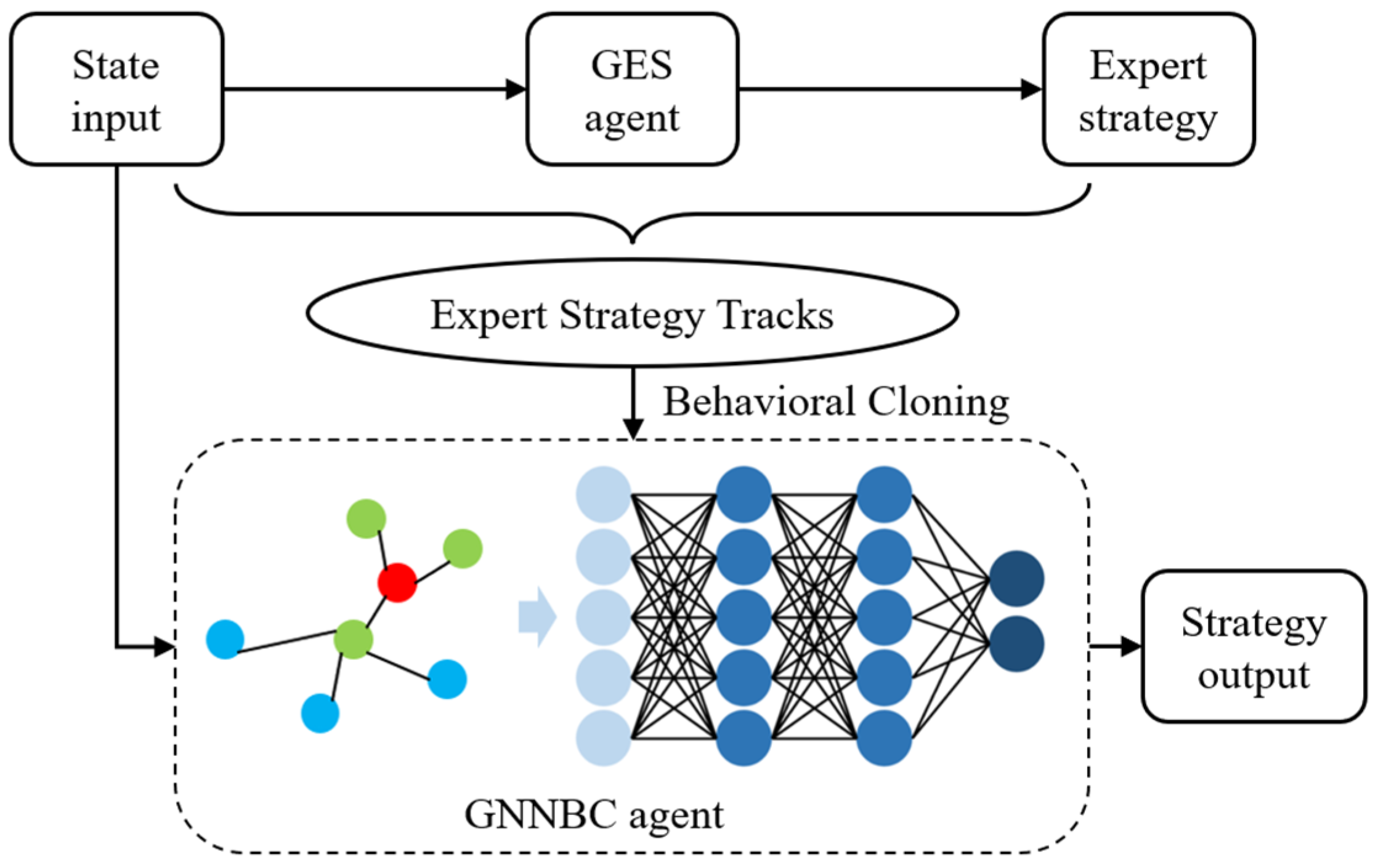
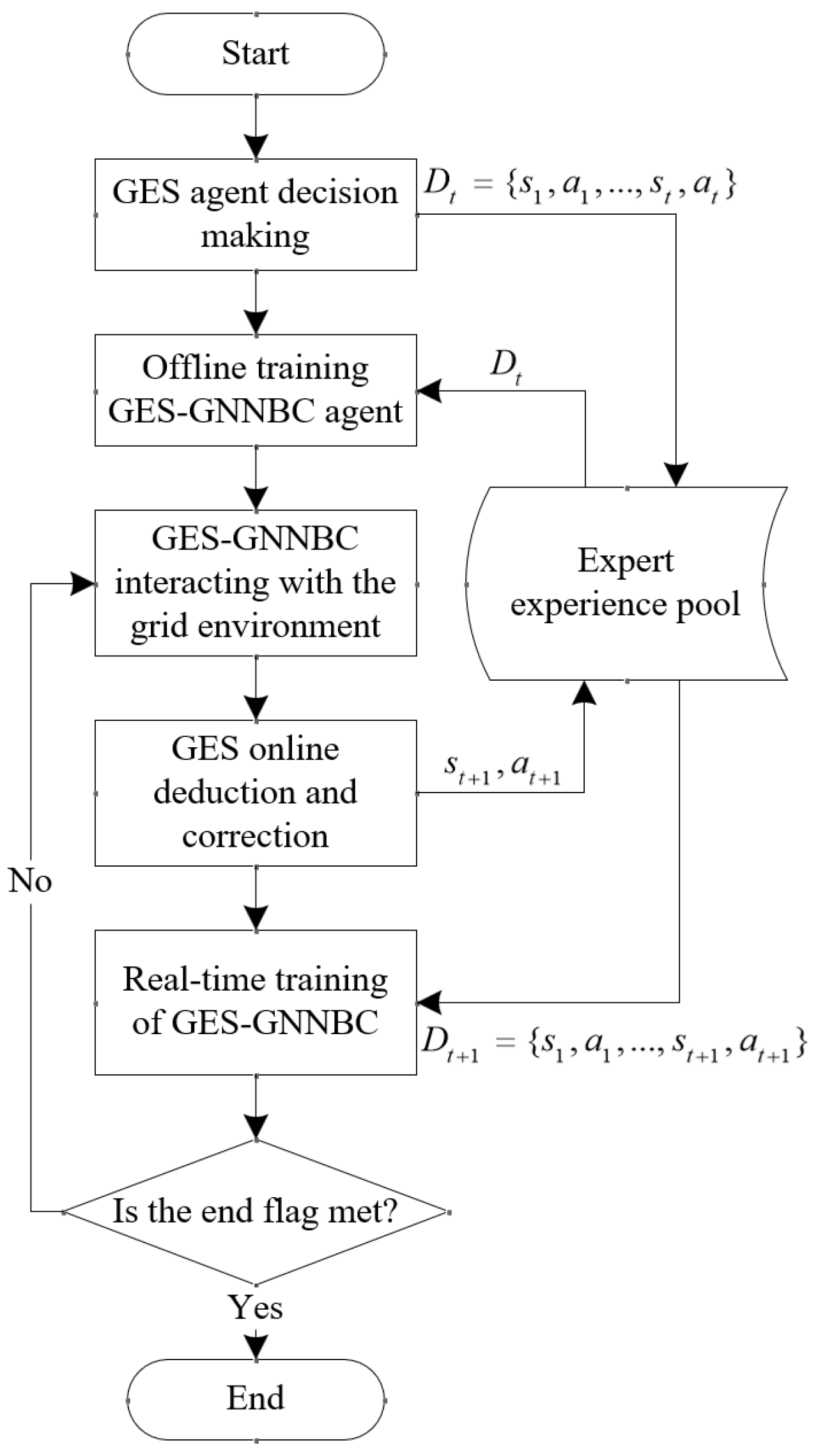
This paper introduces a Grid Expert Strategy-Based Graph Neural Networks Behavioral Cloning (GES-GNNBC) method for real-time power system dispatch. Its main features include: (1) The design of a grid model based on graph theory that provides real-time information on nodes, upstream and downstream unit information on branches, and unit-to-branch connectivity, which can be utilized for the optimization of grid operation. (2) The proposition of a Grid Expert Strategy (GES) that takes into account grid operation optimization and power balance control. This strategy can adjust the active power output of units across the entire grid based on unit-to-branch association information and the full dispatch criteria for renewable energy sources, achieving optimization of grid overload and real-time load rate. Moreover, the strategy allows for the real-time adjustment of the combination of flexible units, balancing system power in real time, and enhancing the safety margin of balancing units. (3) By taking GNN into account, it is able to effectively capture the topological information of the power system, which significantly improves the scheduling accuracy on the basis of the efficient training process of the BC approach. The GES-GNNBC is fused with GES, realizing a model-data-driven GES-GNNBC method for real-time dispatch.

The remainder of this paper is organized as follows: Section 2 introduces the operational rules of the power grid and the foundational technologies related to GES-GNNBC; Section 3 proposes the GES design scheme, including grid modeling based on graph theory and the grid expert strategy; Section 4 presents the GES-GNNBC implementation framework, comprising an introduction to the GNN architecture, the specific design scheme for BC, and the integration and application of GES-GNNBC in real-time power system dispatch; Section 5 validates and compares the proposed methods with an improved IEEE 33-bus system; Section 6 concludes the paper.

2. Problem Formulation

Section 2.1 and Section 2.2 detail the operational constraints of power systems and active power adjustment actions, respectively, serving as the foundation for the design of the action space for GES and GNN-based BC; Section 2.3 introduces the evaluation metrics and reward functions, which will be utilized for the comparison of dispatch results and the training of the A3C algorithm in the case study analysis of Section 5.

2.1. Power System Operational Constraints

The operating constraints on the active output of the generator and the thermal capacity of the grid branch are shown in Equations (1)–(3) [20,21,22,23]:

$${\displaystyle \sum \mathrm{\Delta }}{P}_{gi,t}=\mathrm{\Delta }{P}_D^{t+1}-\mathrm{\Delta }{P}_D^t,\forall i\in G$$

(1)

$$P_{gi}^{\min }\le P_{gi}\le P_{gi}^{\max },\forall i\in G$$

(2)

$$R_l\le R_l^{\max },\forall l\in L$$

(3)

where: $\mathrm{\Delta }{P}_{gi,t}$ denotes the adjusted value of active output of generating unit i at the current moment; $\mathrm{\Delta }{P}_D^{t+1}$ is the forecasted value of ultra-short-term load at the next moment; $\mathrm{\Delta }{P}_D^t$ is the load at the current moment; $G$ denotes the aggregation of generating units; $P_{gi}^{\min }$ and $P_{gi}^{\max }$ denote the lower and upper limits of active output of generating units, respectively; $P_{gi}$ denotes the current active output of generating units; $R_l$ and $R_l^{\max }$ denote the current and maximum load ratios of the branch circuit $l$, respectively; $L$ denotes the set of branches.

2.2. Power System Active Regulation Action

The main active regulation actions of the power system include generator active output adjustment and generator start-stop.

(1)

The margins for generator active output adjustment are shown in Equations (4) and (5):

$$\mathrm{\Delta }{P}_{gi,t}^{\min }\le \mathrm{\Delta }{P}_{gi,t}\le \mathrm{\Delta }{P}_{gi,t}^{\max },\forall i\in G$$

(4)

$$\left\{\begin{array}{ll}{C}_i=0,\hfill & P_{gi}>P_{gi}^{\min }\hfill \\ C_i=1,\hfill & P_{gi}\le P_{gi}^{\min }\hfill \end{array}\right.\forall i\in G$$

(5)

where: $\mathrm{\Delta }{P}_{gi,t}^{\max }$ and $\mathrm{\Delta }{P}_{gi,t}^{\min }$ are the upper and lower limits of the active output of unit i at the current moment, respectively [21]; $\mathrm{\Delta }{P}_{gi,t}$ is the adjusted value of the active output of unit i at the current moment; and $r$ is the climbing rate of the unit.

(2)

Generator start-stop rules are shown in Equations (6) and (7):

$$\left\{\begin{array}{ll}{C}_i=0,\hfill & P_{gi}>P_{gi}^{\min }\hfill \\ C_i=1,\hfill & P_{gi}\le P_{gi}^{\min }\hfill \end{array}\right.\forall i\in G$$

(6)

$$\left\{\begin{array}{ll}{S}_i=0,\hfill & T_{gi}^c\le T_c\hfill \\ S_i=1,\hfill & T_{gi}^c>T_c\hfill \end{array}\right.\forall i\in G$$

(7)

where: $C_i$ and $S_i$ represent whether the start-stop of unit i is allowed or not, respectively; when the active output of the unit is less than or equal to the lower limit of the output, $C_i$ is 1, indicating that the shutdown operation is allowed, otherwise $C_i$ is 0, indicating that the unit is not allowed to be shut down; when the shutdown time $T_{gi}^c$ of the shutdown unit i is greater than or equal to the setpoint value $T_c$, $S_i$ is 1, indicating that the start-up operation is allowed, otherwise $S_i$ is 0, indicating that the start-up is not allowed [21].

2.3. Evaluation Metrics and Reward Function

In order to compare the scheduling results in Section 5, scheduling evaluation metrics and reward functions need to be designed, where the reward functions are also used for training the A3C algorithms to be compared in this paper. The scheduling evaluation indexes are shown in Equations (8)–(10) [9].

$$r_1=1-{\displaystyle \frac{1}{L}}{\displaystyle \sum _{l\in L}\min }(R_l,1)$$

(8)

$$r_2={\displaystyle \frac{P_{\mathrm{r},t}}{P_{\mathrm{r},t}^{\max }}}$$

(9)

$$r_3=-{\displaystyle \sum _{i\in G}(a_i{P}_{\mathrm{g}i}^2+b_i{P}_{\mathrm{g}i}+c_i)}$$

(10)

where: $r_1$, $r_2$, and $r_3$ denote the evaluation of grid security operation, renewable energy utilization rate, and unit operation cost, respectively; $r_1$ and $r_2$ are positive evaluation, and $r_3$ is negative evaluation; $P_{\mathrm{r},t}$ and $P_{\mathrm{r},t}^{\max }$ denote the sum of the active output and the upper limit of the renewable energy unit at the current moment, respectively; $a_i$, $b_i$, and $c_i$ represent the cost coefficients of unit i. Based on the scheduling evaluation indexes (11)–(13), the reward function is constructed as shown in Equations (11) and (12).

$$R_{\mathrm{C}}={\displaystyle \frac{r_3}{C^{\max }}}$$

(11)

$$r_{eward}=\left\{\begin{array}{l}\theta ,\mathrm{power}\mathrm{flow}\mathrm{not}\mathrm{converge}\\ a_1{r}_1+a_2{r}_2+a_3{R}_c,\mathrm{power}\mathrm{flow}\mathrm{converge}\end{array}\right.$$

(12)

where: $R_{\mathrm{C}}$ is the normalization result of $r_3$; $C^{\max }$ is the maximum value of unit operation cost at the current scheduling time step; $r_{eward}$ is the reward value of real-time scheduling decision; $\theta$ is the penalty value of non-convergence of grid currents; $a_1$, $a_2$, and $a_3$ are the reward weighting coefficients; in the new type of electric power system, the safe consumption of renewable energy is the main task, so this paper focuses on the setting of $a_2$ to a larger value, which is generally 2–3 times the rest of the weight, and $a_1$ and $a_3$ are the second priority values.

3. GES Design Scheme

The GES-GNNBC real-time scheduling method needs to consider the design scheme of GES and GNN-based BC. In this section, firstly, a graph-theory-based grid model is constructed, and secondly, a GES is proposed to realize the optimization of grid operation and real-time power balancing.

3.1. Construction of Power Grid Model Based on Graph Theory

The traditional grid fault analysis method is based on a detailed model of the power system for sensitivity analysis, which is computationally intensive to scan all faults and difficult to obtain analysis results in real time. To address the above problems, this section proposes a graph theory-based grid model construction method, which can analyze the correlation information among nodes, units, and branches of the grid in a fast and real-time manner for the grid operation optimization of GES.

The upstream and downstream unit information of the branch to be analyzed can be obtained in real time through the state information of each node, unit, and branch of the grid, as shown in Equations (13)–(17).

$$I=V\cdot B^n\cdot C$$

(13)

$$I=\left[\begin{array}{cccc}{I}_{11}& I_{12}& \dots & I_{1L}\\ I_{21}& I_{22}& \dots & I_{2L}\\ \dots & \dots & \dots & \dots \\ I_{G1}& I_{G2}& \dots & I_{GL}\end{array}\right]$$

(14)

$$V=\left[\begin{array}{cccc}{V}_{11}& V_{12}& \dots & V_{1N}\\ V_{21}& V_{22}& \dots & V_{2N}\\ \dots & \dots & \dots & \dots \\ V_{G1}& V_{G2}& \dots & V_{GN}\end{array}\right]$$

(15)

$$B=\left[\begin{array}{cccc}{B}_{11}& B_{12}& \dots & B_{1N}\\ B_{21}& B_{22}& \dots & B_{2N}\\ \dots & \dots & \dots & \dots \\ B_{N1}& B_{N2}& \dots & B_{NN}\end{array}\right]$$

(16)

$$C=\left[\begin{array}{cccc}{C}_{11}& C_{12}& \dots & C_{1L}\\ C_{21}& C_{22}& \dots & C_{2L}\\ \dots & \dots & \dots & \dots \\ C_{N1}& C_{N2}& \dots & C_{NL}\end{array}\right]$$

(17)

In the equation: $I$ represents a matrix encompassing all branches with upstream and downstream generating units within a range of n pathways (for instance, $I_{GL}$ being positive indicates that generating unit G is upstream of branch L, negative denotes downstream, and zero signifies no upstream or downstream relationship within the n pathways range); $V$ denotes the generator-to-node association matrix, for example, $V_{GN}=1$ indicates a mapping relationship between generating unit G and node N, and $V_{GN}=0$ indicates no mapping relationship; $B$ is the adjacency matrix representing the connectivity between nodes in the power grid, for example, $B_{N2}=1$ signifies a connection between node N and node 22, and $B_{N2}=0$ indicates no connection; $C$ is the node-to-branch association matrix, $C_{NL}=1$ indicates node N is at the start of branch L, $C_{NL}=-1$ indicates the end, and $C_{NL}=0$ indicates no connection.

3.2. Model-Driven GES Power Grid Expert Strategy

Based on the grid model constructed in Section 3.1, this paper proposes a model-driven GES strategy, which includes a grid operation optimization strategy and a power balance control strategy.

3.2.1. Optimization Strategies for Grid Operation

(1)

Grid overload optimization.

Real-time scheduling must perform at least N-1 fault analysis to optimize overloaded lines or lines with overload risk. The overall optimization idea is to adjust the active output of the upstream and downstream units of the overloaded lines in real time, in which the upstream and downstream units’ active outputs can be obtained from the grid model established in Section 2. The specific active output adjustment method is shown in Equations (18) and (19).

$$\left\{\begin{array}{ll}\mathrm{\Delta }{P}_x^{\mathrm{up}}=-\alpha P_x^{\max },\hfill & I_{x,l}>0,x\in X\hfill \\ \mathrm{\Delta }{P}_y^{\mathrm{down}}=\alpha P_y^{\max },\hfill & I_{y,l}<0,y\in Y\hfill \end{array}\right.$$

(18)

$$P_{\mathrm{mark}}={\displaystyle \sum _{x\in X}\mathrm{\Delta }}{P}_x^{\mathrm{up}}+{\displaystyle \sum _{y\in Y}\mathrm{\Delta }}{P}_y^{\mathrm{down}}$$

(19)

where: $\mathrm{\Delta }{P}_x^{\mathrm{up}}$ and $\mathrm{\Delta }{P}_y^{\mathrm{down}}$ are the active output adjustment values of upstream unit $x$ and downstream unit $y$ located in branch $l$ to be treated, respectively; $\alpha$ is the output adjustment coefficient that can be set according to the actual operation of the grid; $X$ and $Y$ are the sets of upstream and downstream units of the branch to be treated, respectively, which are obtained from Equations (13)–(17); and $P_{\mathrm{mark}}$ is the total amount of active imbalance of the units involved in the overload optimization.

(2)

Real-time grid load factor optimization.

In order to reduce the risk of heavy load/overload on the grid due to faults, sudden load increase, and large-scale power output of renewable energy sources, the GES designed in this paper proposes to utilize the grid model to obtain the information on the number of branches of the nodes where generators are located and then adjust the power output of generators in the same proportion in accordance with the number of branches of the nodes where the units are located, so as to reduce the degree of localized heavy load/overload on the lines. In order to make the load ratio of the whole network close to the same level, it is necessary to optimize the generator output according to the number of nodes where generators are connected. The number of generator connection nodes can be obtained from Equation (20).

$$D=V\cdot \mathrm{diag}({\displaystyle \sum _{u\in N}{B}_{u1}},{\displaystyle \sum _{u\in N}{B}_{u2}},\dots {\displaystyle \sum _{u\in N}{B}_{uN}})$$

(20)

where $D$ denotes the information on the number of connected branches at the node where each unit is located, which is obtained by summing $B$ by rows and undergoing diagonalization transformation, and then multiplying it by $V$.

The more nodes a generator is connected to, the greater the capacity of its connected branches to share the generator’s output, and therefore the greater the amplitude of the output to be adjusted. Therefore, after obtaining the predicted ultra-short-term renewable energy output, on the premise of maximizing the consumption of renewable energy in the next scheduling stage, if the renewable energy can be fully generated in the next scheduling stage, the thermal power units will be adjusted according to the number of connecting branches in the nodes in which they are located in the same proportion; if the renewable energy cannot be fully generated in the next scheduling stage, the thermal units will be adjusted according to the “lower limit” of the active output, and the thermal units will be adjusted according to the “lower limit” of the active output. If the renewable energy cannot be fully generated in the next scheduling stage, the thermal power units will be adjusted according to the “lower limit” of the active output, and at the same time, the renewable energy units will be adjusted according to the number of connecting branches in the node. In order to meet the premise of maximizing the consumption of renewable energy, it is necessary to set the renewable energy full generation criterion in real time before optimizing the load ratio of the grid, as shown in Equation (21).

$$P_d=\mathrm{\Delta }{P}_{r,t+1}^{\max }+\mathrm{\Delta }{P}_{T,t+1}^{\min }$$

(21)

where: $P_d$ is the renewable energy full generation criterion; $\mathrm{\Delta }{P}_{r,t+1}^{\max }$ is the sum of the adjustment upper limit of the active output of all renewable energy units at the next moment;$\mathrm{\Delta }{P}_{T,t+1}^{\min }$ is the sum of the adjustment lower limit of the active output of all thermal power units at the next moment.

The specific adjustment method of generator active output is shown in Equations (22) and (23).

$$r_{\mathrm{atio}}=\left\{\begin{array}{l}{\displaystyle \frac{(\mathrm{\Delta }{P}_{\mathrm{adj}}-\mathrm{\Delta }{P}_{r,t+1}^{\max })-\mathrm{\Delta }{P}_{\mathrm{T},t+1}^{\min }}{\mathrm{\Delta }{P}_{\mathrm{T},t+1}^{\max }-\mathrm{\Delta }{P}_{\mathrm{T},t+1}^{\min }}},P_{\mathrm{d}}\le \mathrm{\Delta }{P}_{\mathrm{adj}}\\ {\displaystyle \frac{(\mathrm{\Delta }{P}_{\mathrm{adj}}-\mathrm{\Delta }{P}_{\mathrm{T},t+1}^{\min })-\mathrm{\Delta }{P}_{r,t+1}^{\min }}{\mathrm{\Delta }{P}_{r,t+1}^{\max }-\mathrm{\Delta }{P}_{r,t+1}^{\min }}},P_{\mathrm{d}}>\mathrm{\Delta }{P}_{\mathrm{adj}}\end{array}\right.$$

(22)

$$\mathrm{\Delta }{P}_{\mathrm{gi}}=r_{\mathrm{atio}}(\mathrm{\Delta }{P}_{\mathrm{gi}}^{\max }-\mathrm{\Delta }{P}_{\mathrm{gi}}^{\min }){\displaystyle \frac{D_{\mathrm{gi}}}{\overline{D}}}+\mathrm{\Delta }{P}_{\mathrm{gi}}^{\min }$$

(23)

where: $r_{\mathrm{atio}}$ is the “same proportion” adjustment coefficient of the power output of the unit; $\mathrm{\Delta }{P}_{\mathrm{adj}}$ is the amount of active inequality of the system, which can be obtained from the following Section 3.2.2; $\mathrm{\Delta }{P}_{\mathrm{T},t+1}^{\max }$ is the sum of the upper limit of the adjustment of the power output of all thermal power units; $\mathrm{\Delta }{P}_{r,t+1}^{\min }$ is the sum of the lower limit of the adjustment of all renewable energy units; $D_{\mathrm{gi}}$ denotes the number of branch circuits connected to the node where unit i is located; $\overline{D}$ denotes the average value of $D$.

3.2.2. Power Balance Control Strategy

In order to cope with the steep increase/decrease of renewable energy output and load surge, the power balance control strategy of GES is designed in this section, including the determination of system active imbalance and the optimization of unit regulation capability.

(1)

System Active Unevenness Measure Determination.

First, the maximum value of the next momentary load forecast and the maximum possible generation feed-in loss (the instantaneous output of the largest on-line synchronous machine) is taken as the initial system active inequality measure:

$$\mathrm{\Delta }P=\max \left\{\mathrm{\Delta }{P}_{\mathrm{sg}}^{\max },\mathrm{\Delta }{P}_{\mathrm{D}}^{t+1}-\mathrm{\Delta }{P}_{\mathrm{D}}^t\right\}$$

(24)

where: $\mathrm{\Delta }P$ is the initially determined amount of active system imbalance; $\mathrm{\Delta }{P}_{\mathrm{sg}}^{\max }$ is the maximum possible generation feed-in loss.

Next, the real-time regulation margin of the balancing machine is considered:

$$\mathrm{\Delta }{P}_{\mathrm{b}}=\left\{\begin{array}{l}{P}_{\mathrm{b}}-P_{\mathrm{b}}^{\max },P_{\mathrm{b}}>P_{\mathrm{b}}^{\max }\hfill \\ 0,\hspace{1em}{P}_{\mathrm{b}}^{\min }\le P_{\mathrm{b}}\le P_{\mathrm{b}}^{\max }\hfill \\ P_{\mathrm{b}}-P_{\mathrm{b}}^{\min },P_{\mathrm{b}}<P_{\mathrm{b}}^{\min }\hfill \end{array}\right.$$

(25)

where: $\mathrm{\Delta }{P}_{\mathrm{b}}$ is the amount by which the balancer output exceeds its safety margin constraint, $P_{\mathrm{b}}$ is the balancer output, and $P_{\mathrm{b}}^{\max }$ and $P_{\mathrm{b}}^{\min }$ are the upper and lower limits of the balancer safety margin constraint, respectively.

Then, the amount of active adjustment used for overload optimization (Equation (19)) is removed to determine the final amount of active imbalance of the system:

$$\mathrm{\Delta }{P}_{\mathrm{adj}}=\mathrm{\Delta }P+\mathrm{\Delta }{P}_{\mathrm{b}}-P_{\mathrm{mark}}$$

(26)

(2)

System Balancing Capacity Optimization.

To dissipate the amount of system active imbalance identified above, GES proposes to optimize the system balancing capacity by turning on or off specific units. This is shown in Equations (27) and (28):

$$P_{\mathrm{s}}=\left\{\begin{array}{l}\mathrm{\Delta }{P}_{\mathrm{adj}}-{\displaystyle \sum _{i\in \mathrm{G}}{U}_i^{\mathrm{G}}}\mathrm{\Delta }{P}_{gi}^{\max },\mathrm{\Delta }{P}_{\mathrm{adj}}>0\hfill \\ \mathrm{\Delta }{P}_{\mathrm{adj}}-{\displaystyle \sum _{i\in \mathrm{G}}{U}_i^{\mathrm{G}}}\mathrm{\Delta }{P}_{gi}^{\min },\mathrm{\Delta }{P}_{\mathrm{adj}}<0\hfill \end{array}\right.$$

(27)

$$U_i^G=\left\{\begin{array}{ll}1,\hfill & S_i=1\cap \min |P_s-\mathrm{\Delta }{P}_{gi}^S|,\forall i\in G_{\mathrm{c}}\hfill \\ 0,\hfill & C_i=1\cap \min |P_{\mathrm{s}}-\mathrm{\Delta }{P}_{gi}^{\min }|,\forall i\in G_{\mathrm{o}}\hfill \end{array}\right.$$

(28)

where: $P_{\mathrm{s}}$ is the amount of remaining active inequality to be dissipated; $U_i^{\mathrm{G}}$ is the operating state of unit i, 1 indicates the on state, and 0 indicates the off state; $\mathrm{\Delta }{P}_{gi}^S$ is the climbing power allowed to be turned on for unit i; $G_{\mathrm{c}}$ is the set of units that are turned off; $G_{\mathrm{o}}$ is the set of units that are online.

4. Implementation Scheme of GES-GNNBC in Real-Time Power System Scheduling

In this section, the BC algorithm fused with GNN, forming GNNBC, is used to learn online the GES proposed in Section 3, to realize real-time scheduling of power system based on GES-GNNBC, and to improve the computational efficiency and generalization ability of the scheduling method.

4.1. GNN

The graph structure data can be defined as $G=(V,E)$, where $V$ denotes the set of nodes in the system and $E$ denotes the set of edges in the system. In the neural network model training, the update and representation of nodes are performed by aggregating the information transfer between nodes.

$$h_i^k={\psi }^k\left(h_i^{k-1},{\displaystyle \sum _{j\in \mathcal{N}(i)}{\varphi }^k}(h_i^{k-1},h_j^{k-1},e_{i,j})\right)$$

(29)

where: $h_i^k$ denotes the vector representation of node i after the kth layer of neural network; $\mathcal{N}(i)$ denotes the neighbor nodes of node i; $\psi$,$\varphi$ denote different differentiable functions; $e_{i,j}$ is the feature vector of the edge.

A principal limitation of graph neural network models in the domain of graph representation learning is their susceptibility to oversmoothing when an excessive number of network layers are stacked. This leads to a homogenization of node representations, which in turn diminishes the effectiveness of the training process. To better harness the information encapsulated within graphs and to mitigate the emergence of oversmoothing, this paper introduces the application of an attention mechanism. This mechanism differentially weights neighboring nodes during the aggregation of node information and iteratively updates these weights throughout the training of the model. The relevant formulas are specified as follows.

$$h_i^k={\alpha }_{i,i}W{h}_i^{k-1}+{\displaystyle \sum _{j\in \mathcal{N}(i)}{\alpha }_{i,j}}W{h}_j^{k-1}$$

(30)

where: $W$ denotes the matrix of neural network parameters to linearly transform the node features; ${\alpha }_{i,j}$ is the attention coefficient.

$${\alpha }_{i,j}={\displaystyle \frac{\exp (\mathrm{GELU}(a^{\mathrm{T}}[W{h}_i\Vert W{h}_j\Vert W_e{e}_{i,j}]))}{{\displaystyle \sum _{k\in \mathcal{N}(i)\cup \left\{i\right\}}\exp }(\mathrm{GELU}(a^{\mathrm{T}}[W{h}_i\Vert W{h}_k\Vert W_e{e}_{i,k}]))}}$$

(31)

where: vector $a$ is the parameter vector of the attention network; $W_e$ is the parameter matrix that linearly transforms the edge information; GELU is the activation function; “$\Vert$” is the vector connective.

4.2. Behavioral Cloning

BC comprises four core components: input state, expert and BC intelligences, expert strategies, and intelligence actions. The process begins with the expert intelligence evaluating the input state and deriving an expert strategy, known as the expert strategy trajectory. Unlike the traditional RL approach that relies on stochastic exploration to find the optimal strategy trajectory [24], BC intelligently learns from the demonstrated expert strategy trajectory, enhancing training efficiency. The BC algorithm employs supervised learning to annotate expert demonstrations and trains the intelligence to achieve the optimal strategy. This paper suggests applying this training approach for online learning of GES, detailed in Section 3.

4.3. Specific Design Scheme of GNNBC

4.3.1. Networks Structure Design

The advantage of fusing GNN and BC to obtain GNNBC is that GNN is able to extract the information in the topology, which further accelerates the efficiency of BC model mimicry training and further improves the accuracy of mimicry, and the structure of GNNBC is shown as Figure 1. The structure of the BC model includes feature engineering, an input layer, a hidden layer, and an output layer, in which the feature engineering network is GNN. After obtaining the grid operation state, BC uses an encoder to classify the grid state information and then goes through the GNN to perform the feature extraction, inputs the result of the feature extraction into the neural network, and finally outputs the scheduling decision. The activation functions used in the hidden layer and output layer are ReLU and Tanh, respectively.

4.3.2. State Space

The design of the state space should consider the relevant information that can influence the scheduling decision, and the state space of BC is constructed as shown in Equation (32) based on the grid state information utilized by the GES in Equations (13)–(28).

$$S=[B,C,V,I,P_G,R,\mathrm{\Delta }{P}_{G,t+1}^{\max },\mathrm{\Delta }{P}_{G,t+1}^{\min },T_C,P_r^{\max },\mathrm{\Delta }{P}_D^{t+1},U^{\mathrm{G}},U^{\mathrm{L}},t]$$

(32)

where: $S$ denotes the state space of GNNBC; $B,C,V,I$ are mentioned in Section 3, which are utilized to catch the grid topological structure; $P_G$ is the set of unit active outputs; $R$ is the set of branch load ratios; $\mathrm{\Delta }{P}_{G,t+1}^{\max }$ and $\mathrm{\Delta }{P}_{G,t+1}^{\min }$ denote the set of upper and lower bounds of active outputs of all units in the next moment of the active outputs action space; $T_C$ is the set of remaining time allowed for re-start of shutdown units; $P_r^{\max }$ is the set of renewable energy output prediction; $\mathrm{\Delta }{P}_D^{t+1}$ is the value of ultra-short-term load prediction; $U^{\mathrm{G}}$ is the set of unit statuses; $U^{\mathrm{L}}$ is the set of branch states; and t denotes the current running time step.

4.3.3. Action Space

According to Equations (2)–(7), the action space of BC intelligences satisfying the grid operation constraints is constructed as shown in Equation (33):

$$A=[U_1^{\mathrm{G}}\mathrm{\Delta }{P}_{\mathrm{g}1},U_2^{\mathrm{G}}\mathrm{\Delta }{P}_{\mathrm{g}2},\dots ,U_i^{\mathrm{G}}\mathrm{\Delta }{P}_{\mathrm{g}i}]$$

(33)

where $A$ is the action space of BC, including the active output adjustment of generator and generator start/stop.

4.3.4. Loss Function Design

The grid state information utilized by the GES is denoted as $s$, and the generated scheduling policy is denoted as $a$. $s$ is used as the input data of the GNNBC, and $a$ is used as the labeled data for the GNNBC intelligences training, and the training process can be formulated as a regression problem. The first-order optimization method of stochastic gradient descent is used to train the GNNBC’s scheduling policy trajectory $\pi (s)$. Since the optimization stage of the system balancing capacity in GES is a classification problem and the conventional loss function is difficult to learn, a penalty function is added to the loss function according to Equations (30) and (31), as shown in Equation (34):

$$\begin{array}{l}L(\theta )={\displaystyle \frac{1}{J}}{\displaystyle \sum _{j=1}^J||\pi (s_j)-a_j|{|}_2^2}\\ +{\displaystyle \frac{\lambda }{J}}{\displaystyle \sum _{j=1}^J||({\mu }_j-U_j^{\mathrm{G}})(\pi (s_j)-a_j)|{|}_2^2}+{\displaystyle \frac{\beta }{2}}{\Vert \theta \Vert }_2^2\end{array}$$

(34)

where: $\theta$ denotes the network parameters of GNNBC; $J$ denotes the training batch size; ${||\cdot ||}_2^2$ denotes the square of the Euclidean paradigm; $\lambda$ is the penalization factor; ${\mu }_j$ denotes the array with the value of 1 and the length the same as that of $U_j^{\mathrm{G}}$; and $\beta$ is the greater than 0 constant. The first term is the loss function of the GNNBC scheduling policy trajectory $\pi (s_j)$ with respect to the GES scheduling policy $a_j$; the second term is the penalty function established for the optimization phase of the system balancing capacity in the GES; and the third term is the L2 regularity term, which prevents the GNNBC from being overfitted during training.

4.4. Integration and Application of GES-GNNBC in Real-Time Power System Scheduling

The specific method steps of GES-GNNBC with real-time grid scheduling system are shown in Figure 2. The specific steps are: (1) The GES interacts with the grid environment to generate $t$ groups of grid states $s$ and expert policies $a$, which are deposited into the expert experience pool. (2) The GNNBC intelligences of the fused GNN are trained offline using the data $D_t$ of the expert experience pool and the GNNBC algorithm. (3) The GNNBC interacts with the grid environment to generate the scheduling policy $\pi (s_t)$ based on the current grid state $s_t$ and returns to the grid environment to obtain the next grid state $s_{t+1}$. (4) The GES processes the grid state $s_{t+1}$, generates the expert policy $a_{t+1}$, and updates the expert experience pool to $D_{t+1}$ in real time, realizing the online demonstration and correction of GNNBC by the GES. (5) The GNNBC learns the GES using the $D_{t+1}$, realizing the application of GES-GNNBC in the real-time power grid scheduling system.

5. Case Study

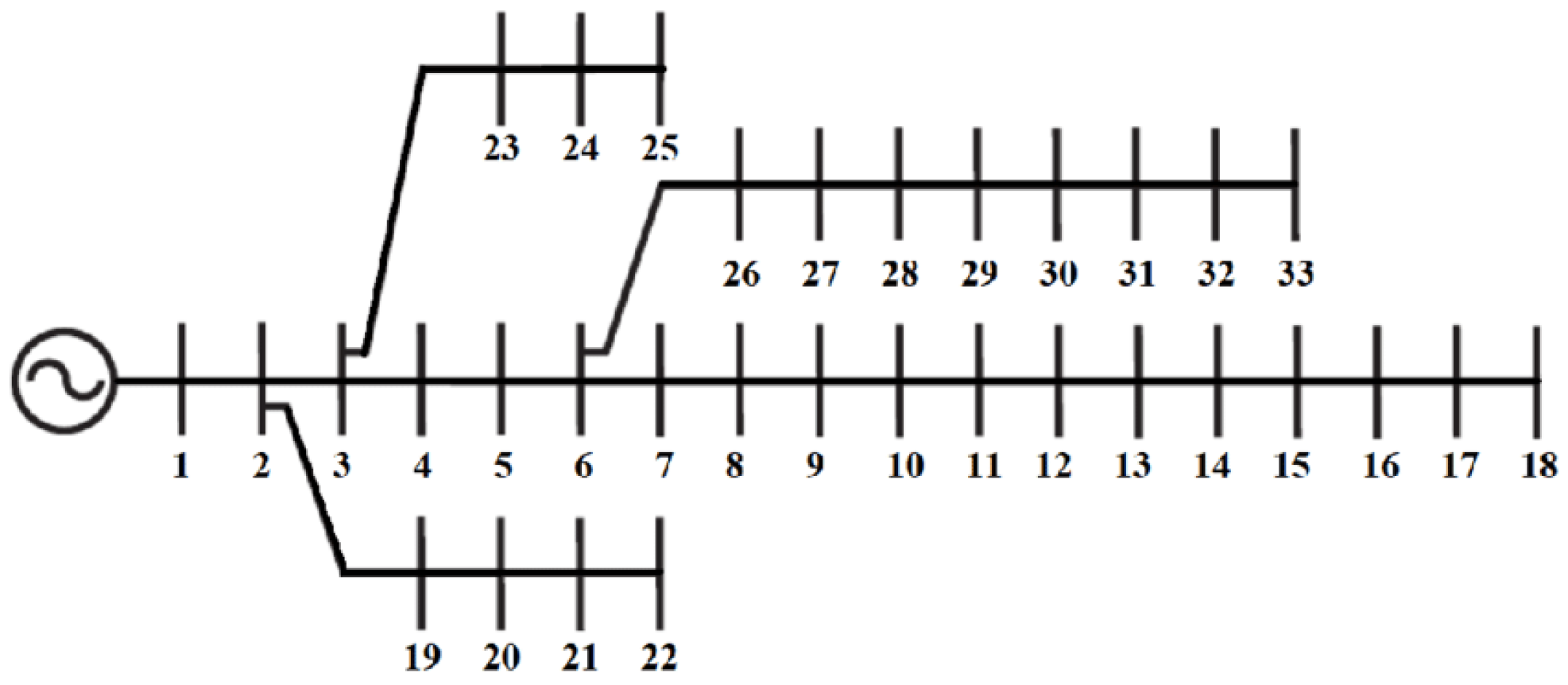
To verify the effectiveness of the GES-GNNBC method, this paper conducts a case study based on the IEEE 33-bus standard system. The IEEE 33-bus test system, derived from the MATPOWER 7.1 toolbox, comprises 1 generator unit, 32 transmission lines, and 32 load nodes. To simulate the output of renewable energy units, this paper modifies the 33-bus system by replacing the unit at node 29 with a photovoltaic power station and the unit at node 15 with a wind farm, as illustrated in Figure 3.

The rated capacity of the renewable energy units is 1.3 times that of the original synchronous units, and the modified system achieves a high proportion of renewable energy installed capacity at 28.1%. The output of renewable energy and load data are based on publicly available data from the California power grid in March, June, September, and December 2021 [25]. To align with the IEEE 33-bus system, the renewable energy output data are proportionally adjusted to 25% of the actual data, and the load data are adjusted to 20% of the actual figures.

This paper utilizes PYPOWER 5.1.17, a Python 3.9 version of the widely used MATPOWER, as a grid environment simulator. Setting $r=0.05$ in Equation (4), $T_c=40(200\min )$ in Equation (7), $n=2$ in Equation (16), $\alpha =0.05\mathrm{pu}$ in Equation (22), and $P_b^{\max }$, $P_b^{\min }$ in Equation (28) are 0.57 pu, 0.43 pu, respectively. The loss function required for GES-GNNBC training is shown in Equation (34) where $\lambda$ is set to be 2 and $\beta$ is 0.02. The reward function is shown in Equation (15), where $\theta =-10$ and $a_1$, $a_2$, and $a_3$ are 1, 2, and 1, respectively.

In order to verify the training efficiency and generalization ability of GES-GNNBC, this study analyzes the performance of the traditional expert method (TEM) [4], the A3C-based grid scheduling method [12], and the GES-GNNBC method proposed in this paper so as to compare and analyze the three approaches in terms of the grid operation optimization and power balance control capabilities.

5.1. Experimental Settings

In terms of expert experience data collection, according to the state space S and action space A in Equations (32) and (33), each group of expert experience data includes the real-time state of the grid and the scheduling policy. In this paper, we take the 288 groups of GES input-output data with 5-min intervals as one scheduling day and randomly select 25 scheduling days per month in March, June, September, and December, and finally obtain a total of 28,800 groups of expert experience. The GNN-GES input-output data are randomly selected from 25 scheduling days in each month of March, June, September, and December and processed with GES to obtain a total of 28,800 sets of expert experiences.

First, GES-GNNBC is trained offline using expert experience data and the BC algorithm for 10,000 iterations; second, to demonstrate the stability of GES-GNNBC during the training process, A3C is trained for the same long training period as GES-GNNBC. Since the TEM scheme does not require training and does not have convergence problems, this section only compares the training convergence of GES-GNNBC in the BC algorithm training phase and A3C.

5.2. Training Convergence Comparison

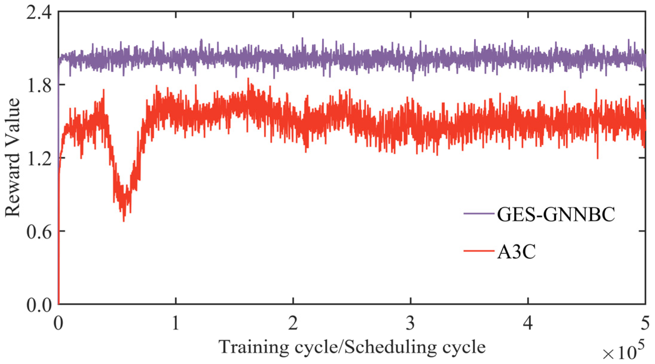
The results of the training convergence comparison between the GES-GNNBC and A3C algorithms are shown in Figure 4. The reward value is the average reward value of a single decision within a scheduling day; considering the variability of the scheduling scenarios, the reward value has a certain degree of reasonable oscillation under both algorithms. In terms of training results, GES-GNNBC reaches a high reward value of 1.96 at the beginning of training, and then after BC algorithm training, the reward value is further improved, and the training converges stably after 2000 scheduling cycles, with an average value of 2.02; whereas the A3C algorithm, even after 7500 scheduling cycles, still has a lower reward value than that of the GES-GNNBC, with an average value of 1.54. In terms of training time, the reward value is the average reward value of a single decision within a scheduling day, with a reasonable degree of oscillation, considering the differences in scheduling scenarios. In terms of training time, GES-GNNBC takes 1.2 h to reach the stable convergence condition (2000 scheduling cycles), while A3C takes 22.4 h to train, which is a significant increase in training speed. In conclusion, the training efficiency of GES-GNNBC is better than that of the A3C algorithm, and it has more potential to be applied in the real-time scheduling of power systems.

5.3. Comparison of Generalization Capability

In order to verify the generalization capability of the proposed GES-GNNBC, this paper selects six large grid disturbance events as test events to test and compare the three scheduling schemes, including: (1) three branch N-1 fault scenarios, which are the faults of lines 5, 12, and 19, respectively; (2) two renewable energy output steep rise/steep fall scenarios, with the range of the steep rise/steep fall accounting for the total generation ±15%; and (3) one load surge scenario with a surge range of 10%.

The grid simulator runs and solves the grid currents based on the scheduling decisions returned by the intelligentsia, stipulating that if the currents do not converge, the current scheduling scenario is judged to be non-convergent, and the comparison results are shown in

Table 1. Comparison results of generalization ability.

Algorithm	Convergence Number	Reward	Renewable Energy Utilization
GES-GNNBC	6	173.26	99.98%
TEM	4	128.52	99.96%
A3C	3	88.47	91.68%

, where the average reward value is the total reward value in a scheduling cycle. As shown in Table 1, GES-GNNBC has a scenario convergence number of 6, which is able to converge in all the scheduling scenarios, while TEM and A3C algorithms have a scenario convergence number of 4 and 3, respectively. The results indicate that, as previously discussed, the TEM approach exhibits inherent rigidity and limited adaptability, failing to effectively accommodate the current power grid landscape characterized by high penetration rates of renewable energy sources. Meanwhile, the A3C framework demonstrates conventional RL methodologies encountering significant training challenges, thereby exhibiting compromised performance capabilities under such operational conditions. The average reward value of GES-GNNBC is 173.26, while TEM and A3C algorithms are 128.52 and 88.47, respectively. It can be seen that GES-GNNBC obtains a much higher reward value than the other two algorithms. In terms of renewable energy utilization, both GES-GNNBC and TEM are better, with 99.98% and 99.96%, respectively, while the A3C algorithm is lower than the first two algorithms, with 91.68%. Based on the data comparison, it can be seen that the grid operation optimization capability of GES-GNNBC can get higher branch optimization rewards and renewable energy utilization rewards; moreover, the power balance control strategy of GES-GNNBC can make the scheduling decision more robust when coping with the scenarios of renewable energy output steeply rising/decreasing, load surge, and generator dropping out; at the same time, the GES-GNNBC is based on the online learning of the GES, which is better than A3C, and the GES-GNNBC is more intelligent. Meanwhile, GES-GNNBC is based on GES for online learning, and compared with the A3C algorithm, the GES-GNNBC intelligent body model converges and is more stable. Therefore, GES-GNNBC has better generalization ability than TEM and A3C.

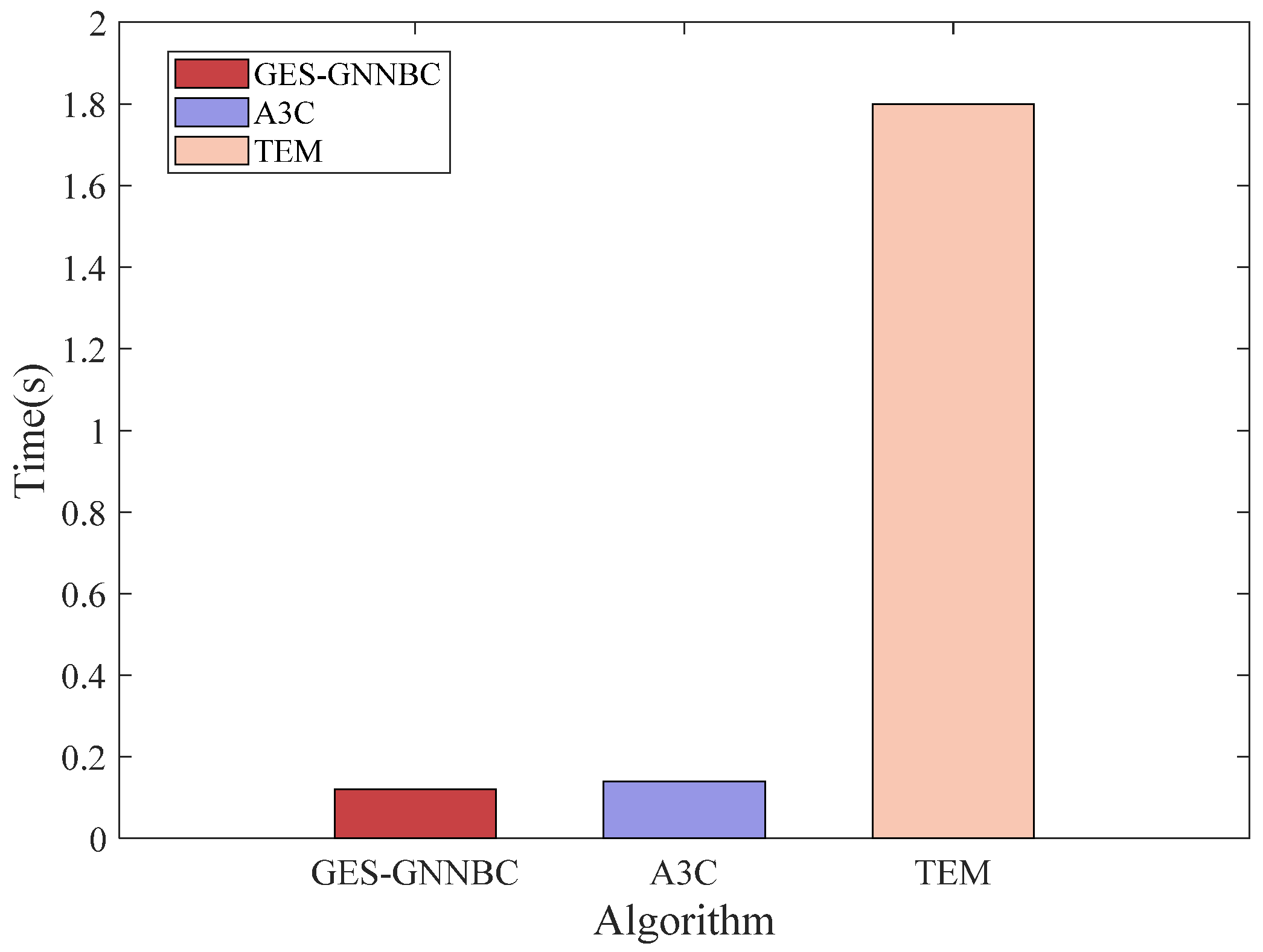
5.4. Decision Time Comparison

In order to analyze the solution efficiency of the scheduling methods, the single-step decision-making time of the three schemes is compared. The computer platform used is the 13th Gen Intel(R) Core(TM) i5-13490F 2.50 GHz with 16 GB of RAM, and the average single-step decision-making time is shown in Figure 5. The traditional TEM method takes 1.8 s, while the GES-GNNBC and A3C take 0.12 s and 0.14 s, respectively, and the decision-making time of the GES-GNNBC is improved by 15 times compared with that of the TEM. Although the time consumed by the GES-GNNBC and A3C algorithms are close to each other, the A3C algorithm is inferior to GES-GNNBC in terms of training efficiency and generalization ability in the analysis of this paper; therefore, it proves that the efficiency of GES-GNNBC is high when it is applied to the real-time security scheduling of electric power systems.

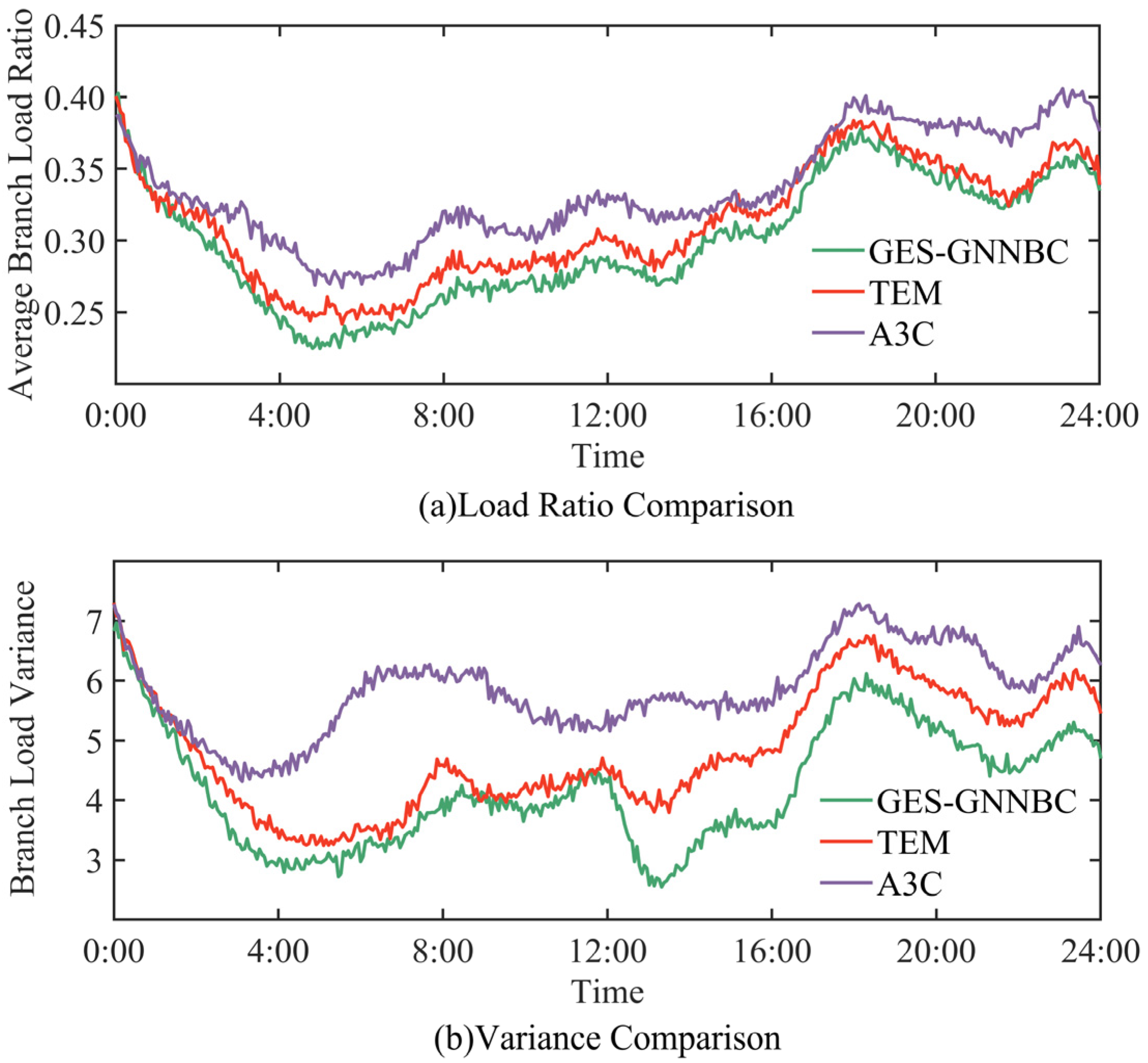
5.5. Grid Load Optimization Comparison

In order to reflect the advantages of GES-GNNBC real-time scheduling, this section reflects the advantages of GES-GNNBC’s grid operation optimization strategy in terms of grid load rate optimization comparison and contrast.

The data of March 5 were selected as the test scenario to compare the grid load optimization capability of GES-GNNBC, TEM, and A3C, and the results are shown in Figure 6. Figure 6 shows the comparison of the average values of the branch load factor of the whole network at multiple time points in the scheduling cycle, and the average value of the branch load factor of GES-GNNBC is significantly lower than that of the TEM and A3C algorithms because GES-GNNBC is able to make the branches with large transmission capacity carry more power loads. Figure 6 shows the comparison of the variance of the algorithms, which represents the uniformity of the branch load, and the variance of the branch load of GES-GNNBC is significantly lower than that of the TEM and A3C algorithms. Therefore, GES-GNNBC is able to reduce the grid loading rate, improve the uniformity of grid current distribution, and enhance the grid transmission utilization.

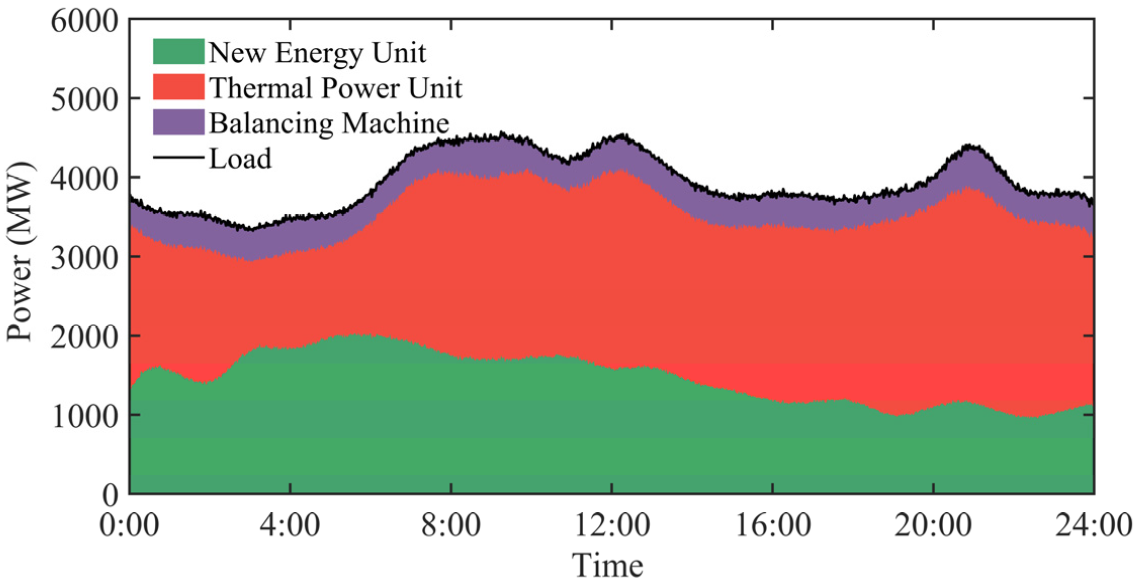
The data of March 17 is selected as the test scenario, and GES-GNNBC is utilized for real-time scheduling, and the scheduling results are shown in Figure 7. During 00:00–06:00, when the renewable energy output is high and the load demand is low, GES-GNNBC prioritizes meeting the load through renewable energy sources and reduces the thermal unit output; During 08:00–10:00, 11:00–12:00, and 20:00–21:00 h, when the load demand is high and the renewable energy output is low, GES-GNNBC meets the power balance by increasing the output of thermal power units. At the same time, GES-GNNBC keeps the balancer’s output locked around the neutral point of 395 MW (the balancer’s power operation range is 338–452 MW), maximizing the balancer’s real-time safety regulation margin.

In summary, GES-GNNBC can improve the robustness of the power system dispatching decision by fully considering grid operation optimization and power balance control. At the same time, GES-GNNBC’s online learning method can greatly improve the training efficiency and computational efficiency of intelligent algorithms and ensure a high degree of real-time scheduling decisions.

6. Conclusions

This paper introduces a novel real-time power system scheduling method named Grid Expert Strategy Behavioral Cloning (GES-GNNBC), leveraging graph neural networks to overcome the limitations of traditional model-driven and data-driven scheduling methods, which suffer from low efficiency and poor generalization. GES-GNNBC integrates a graph theory-based grid model with a grid expert strategy to optimize grid operations and power balance in real-time. Comparative analysis shows that GES-GNNBC outperforms traditional methods by improving grid load management, enhancing current distribution uniformity, and increasing transmission utilization. Additionally, GES-GNNBC demonstrates superior training speed and generalization capability through online learning. The method holds promise for managing the increased scale of renewable energy connections in modern power systems, ensuring real-time grid security, and maximizing renewable energy consumption. Future work will explore its application in day-ahead and intra-day rolling scheduling scenarios.

References

1. Tju, P.; Zhou, X.; Chen, W.; Yu, Y.; Qin, C.; Li, R.; Wang, C.; Dong, X.; Liu, J.; Wen, J. “Smart grid plus” research overview. Electr. Power Autom. Equip. 2018, 38, 2–11. (In Chinese) [Google Scholar]
2. Yang, M.; Cheng, F.; Han, X. Real-time dispatchbased on effective steady-state security regions of power system. Proc. CSEE 2015, 35, 1353–1362. (In Chinese) [Google Scholar]
3. Tang, Y.; Dvijotham, K.; Low, S. Real-time optimal powerflow. IEEE Trans. Smart Grid 2017, 8, 2963–2973. [Google Scholar] [CrossRef]
4. Ross, D.W.; Kim, S. Dynamic economic dispatch of generation. IEEE Trans. Power Appar. Syst. 1980, PAS-99, 2060–2068. [Google Scholar] [CrossRef]
5. Huang, T.; Guo, Q.; Sun, H.; Zhao, N.; Wang, B.; Guo, W. Hybrid modeland data driven concepts for power system security feature selectionand knowledge discovery: Key technologies and engineering application. Autom. Electr. Power Syst. 2019, 43, 95–101+208. (In Chinese) [Google Scholar]
6. Zhang, Q.; Wang, X.; Yang, T.; Ren, J.; Zhang, X. A robustdispatch method for power grid with wind farms. Power Syst. 2017, 41, 1451–1459. (In Chinese) [Google Scholar]
7. Fu, Y.; Lu, M. Scenario decomposition method formulti-objective stochastic dynamic economical dispatch problem. Autom. Electr. Power Syst. 2014, 38, 34–40. (In Chinese) [Google Scholar]
8. Wang, Z.; Shen, C.; Liu, F.; Wu, X.; Liu, C.C.; Gao, F. Chance-constrained economic dispatch with non-Gaussian correlated wind power uncertainty. IEEE Trans. Power Syst. 2017, 32, 4880–4893. [Google Scholar] [CrossRef]
9. Zhou, Y.; Zhang, B.; Xu, C.; Lan, T.; Diao, R.; Shi, D.; Wang, Z.; Lee, W.J. A data-driven methodfor fast AC optimal power flow solutions via deep reinforcement learning. J. Mod. Power Syst. Clean Energy 2020, 8, 1128–1139. [Google Scholar] [CrossRef]
10. Buivh Hussain, A.; Kimh, M. Double deep Q-learning-based distributed operation of battery energy storage system considering uncertainties. IEEE Trans. Smart Grid 2020, 11, 457–469. [Google Scholar]
11. Peng, L.; Sun, Y.; Xu, J.; Liao, S.; Yang, L. Self-adaptive uncertainty economic dispatch based on deep reinforcement learning. Autom. Electr. Power Syst. 2020, 44, 33–42. (In Chinese) [Google Scholar]
12. Qiao, J.; Wang, X.; Zhang, Q.; Zhang, D.; Pu, T. Optimal dispatch ofelectricity-gas system with soft actor-critic deep integrated reinforcement learning. Proc. CSEE 2021, 41, 819–832. (In Chinese) [Google Scholar]
13. Paine, T.L.; Gulcehre, C.; Shahriari, B.; Denil, M.; Hoffman, M.; Soyer, H.; Tanburn, R.; Kapturowski, S.; Rabinowitz, N.; Williams, D.; et al. Making efficient use of demonstrations to solve hard exploration problems. arXiv 2019, arXiv:1909.01387. [Google Scholar] [CrossRef]
14. Sun, W.; Venkatraman, A.; Gordon, G.J.; Boots, B.; Bagnell, J.A. Deeply AggreVaTeD: Differentiable imitation learning for sequential prediction. In Proceedings of the 34th Itemational Conference on Machine Learning, Sydney, Australia, 6–11 August 2017; pp. 3309–3318. [Google Scholar]
15. Osa, T.; Pajarinen, J.; Neumann, G.; Bagnell, J.A.; Abbeel, P.; Peters, J. An algorithmic perspective on imitation learning. Found. Trends Robot. 2018, 7, 1–179. [Google Scholar] [CrossRef]
16. Hussein, A.; Gaber, M.M.; Elyan, E.; Jayne, C. Imitation learning: A survey of learning methods. ACM Comput. Surv. 2018, 50, 21. [Google Scholar] [CrossRef]
17. Wang, X.; Ning, Z.; Guo, S.; Wang, L. Lmitation leamingenabled task scheduling for online vehicular edge computing. IEEE Trans. Mob. Comput. 2022, 21, 598–611. [Google Scholar] [CrossRef]
18. Wu, Z.; Pan, S.; Chen, F.; Long, G.; Zhang, C.; Philip, S.Y. A comprehensive surveyon graph neural networks. IEEE Trans. Neural Netw. Learn. Syst. 2020, 32, 4–24. [Google Scholar] [CrossRef]
19. Liao, W.; Yu, Y.; Wang, Y.; Chen, J. Reactive power optimization of distribution network based on graph convolutional network. Power Syst. Technol. 2021, 45, 2150–2160. [Google Scholar]
20. Huang, L.; Wang, Y.; Guo, J.; Xu, G.; Di, F. Economic dispatchfor disaster prevention considering load rate homogeneity of powergrid and N-1 security constraints. Autom. Electr. Power Syst. 2020, 44, 56–63. (In Chinese) [Google Scholar]
21. Liu, X.C.; Wang, B.B.; Li, Y.; Sun, Y.J. Unit commitment model and economic dispatch model based on real time pricing for power accommodation. Power Syst. Large-Scale Wind Technol. 2014, 38, 2955–2963. (In Chinese) [Google Scholar]
22. Cui, Y.; Zhang, J.; Zhong, W.; Wang, Z.; Zhao, Y. Scheduling strategy of wind penetration multi-source system considering multi-time scalesource-load coordination. Power Syst. Technol. 2021, 45, 1828–1836. (In Chinese) [Google Scholar]
23. Zhang, J.; Wang, P.; Cheng, Z. Multi-objective dispatching adopting chaos particle swarm optimization cooperate with interior point method. Power Syst. Technol. 2021, 45, 613–621. (In Chinese) [Google Scholar]
24. Ross, S.; Gordon, G.; Bagnell, D. A reduction of imitation learning and stmictured prediction to no-regret online learning. In Proceedings of the Fourteenth International Conference on Artificial Intelligence and Statistics, Fort Lauderdale, FL, USA, 11–13 April 2011; pp. 627–635. [Google Scholar]
25. California ISO, Todays California ISO Website. 2007, Volume 3, pp. 154–196. Available online: http://www.caiso.com/todays-outlook/supply (accessed on 22 January 2022).
Figure 1. Schematic diagram of the structure of GNNBC.
Energies 18 01934 g001
Figure 2. Implementation of GES-GNNBC in real-time grid dispatch.
Energies 18 01934 g002
Figure 3. IEEE 33 bus test system.
Energies 18 01934 g003
Figure 4. Comparison of algorithm convergence.
Energies 18 01934 g004
Figure 5. Time comparison of single-step decision.
Energies 18 01934 g005
Figure 6. Comparison results of grid load optimization.
Energies 18 01934 g006
Figure 7. GES-GNNBC scheduling results.
Energies 18 01934 g007