Non-Fault Detection Scheme Before Reclosing Using Parameter Identification for an Active Distribution Network

Abstract

The distribution network line has the risk of an unsuccessful three-phase blind reclosing in permanent fault. Based on the response of the inverter of the distributed generation (DG) to the short-term low-frequency voltage disturbance to the line to be detected, this paper proposes a non-fault identification method for the distribution network before three-phase reclosing, based on model parameter identification. During the disturbance period, when there is no fault after the arc is extinguished, the detection line is three-phase symmetrical, and each phase-to-ground loop is its own loop resistance and inductance linear network, which is independent of the fault location, transition resistance and other factors. Furthermore, the R–L network without fault is used as the identification reference model, and the least squares algorithm is used to identify the resistance and inductance parameters of each phase loop of the detection line by using the voltage and current response information of the line side during the excitation period so as to identify the fault state. The non-fault criterion before three-phase reclosing, characterized by the difference between the calculated value of resistance and inductance and the corresponding actual value, is designed. Finally, PSCAD is used to build a distribution network with DG for verification, and simulations under different fault locations and transition resistances are carried out. The results show that when the line is in a non-fault state, the parameter identification results of the three phase-to-ground circuits are highly consistent with the true value; that is, the non-fault state is determined. When the fault continues, there is a large deviation between the parameter identification results of at least one phase-to-ground loop and the corresponding real value, which does not meet the condition of the non-fault criterion. The method in this paper is more sensitive than the detection method using response voltage. Moreover, it is not necessary to add additional disturbance sources, which is expected to improve the economy and feasibility of three-phase adaptive reclosing applications for distribution lines with a large number of DGs.

1. Introduction

With the rapid development of clean and renewable distributed generation (DG) [1,2], traditional passive distribution networks have become active networks, and this transformation not only improves the complexity and diversity of the distribution network [3], but also brings new challenges to the traditional protection and fault handling modes. Relevant statistics show that more than 80% of the faults occurring in distribution networks are transient faults [4], so the use of pre-accelerated reclosing can significantly shorten the outage time and further improve the reliability of the power supply in distribution networks. The current main strategy for DG access is to increase the check no-voltage step, but since most of the existing distribution network lines are configured with circuit breakers only on the system side, the implementation of check no-voltage usually requires the new energy downstream of the fault point to stop operation, and the reclosing on the permanent fault may cause a secondary impact on the system, further worsening the fault condition and aggravating the damage to the equipment [5].

In order to overcome this shortcoming of traditional auto-reclosure, scholars have proposed adaptive reclosing that identifies the nature of the fault before the circuit breaker recloses so as to avoid reclosing on the faulty line [6]. At present, a lot of research on high-voltage transmission line adaptive reclosing technology is being carried out [7,8,9,10]; the voltage level and structure of distribution lines are obviously different from the transmission line [11], resulting in transmission line existing fault detection technology directly used in the distribution network effect not being ideal. Therefore, there is a need to study adaptive reclosing methods for distribution networks. Existing fault detection methods for distribution networks are divided into two main categories: one is the fault detection technique using the line’s own electrical quantity [12], but this is susceptible to fault location and transition resistance and is difficult to measure when the electrical quantity decays too fast. The second category comprises mainly fault detection techniques using applied disturbance devices, which utilize the response characteristics of the line with respect to applied disturbances for phase-to-phase fault discrimination [13,14]. One of the methods in this category is based on the scheme of identifying the nature of faults by perturbation signals from traditional electrical equipment. Ref. [15] uses a DC source to cast a pre-charged additional capacitor to the fault line several times and screens the fault circuit according to the attenuation characteristics of the capacitor current. In [16], the external disturbance is applied to three phase-to-phase circuits in turn. The fault circuit is identified by the significant difference between the disturbance current of the fault phase-to-phase circuit and the other two non-fault phase-to-phase circuits. The disturbance signal is further applied to the fault phase-to-phase circuit, and the fault type is identified by the difference between the two disturbance currents. The other method is based on the high controllability of power electronic equipment to provide effective fault characteristics for fault screening. Ref. [17] adds the inverter power supply to the distribution transformer and uses the relationship between the line wave impedance and frequency to identify the faulty line. Ref. [18] applies a voltage perturbation signal to the grid using the inverter power supply and estimates the resistance and inductance at the excitation end through parameter identification techniques, and then compares the parameter values obtained from the estimation with the real values of the actual circuit. The estimated parameter values are compared with the real values of the actual circuit to discern the nature of the fault. The use of the external perturbation fault detection scheme has become an effective way to solve the lack of available signals after the tripping of distribution lines, but requires additional configuration of the corresponding dedicated perturbation source. Along with a large number of distributed DGs accessing the distribution network, it has become possible to apply short-duration perturbation excitation using the additional control of the line-accessed DG’s own power electronics after the tripping of the system-side circuit breaker after a fault [19], which provides a new way of thinking in implementing the injective fault detection scheme.

In view of the lack of available and stable electrical information for fault state detection before three-phase reclosing in the present distribution network, this paper uses the additional control characteristics of power electronic links such as distributed power inverters to access the active distribution network itself to generate the feature information for fault detection. After the three-phase tripping of the fault line outlet switch in the distribution network, the three-phase symmetrical low-frequency voltage excitation signal is injected into the line by the self-connected DG. Based on the principle of parameter identification [20,21], the difference between the resistance and inductance identification values and the actual values of each phase loop is used to identify the fault-free state, and the correctness and effectiveness of the method are verified by a large number of simulations.

The rest of the paper is structured as follows. In Section 2, fault characterization of DG-injected faulty lines is performed. Section 3 describes the principle, criterion and basic process of fault-free detection based on parameter identification. In Section 4, the applicability of the method is verified by simulation calculations. Section 5 highlights the effectiveness of the method proposed in this paper based on comparative experiments with other methods. Section 6 summarizes the whole paper. Section 7 discusses the shortcomings of this paper and the main directions for subsequent work.

2. Fault Characterization

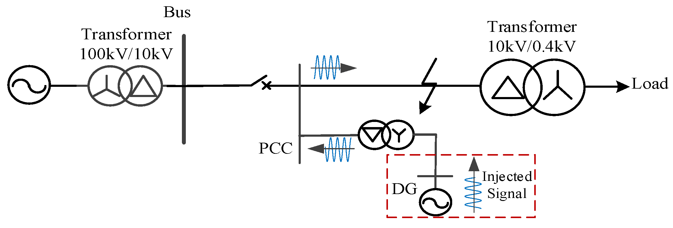
2.1. Fault Detection Scheme Using DG Injection

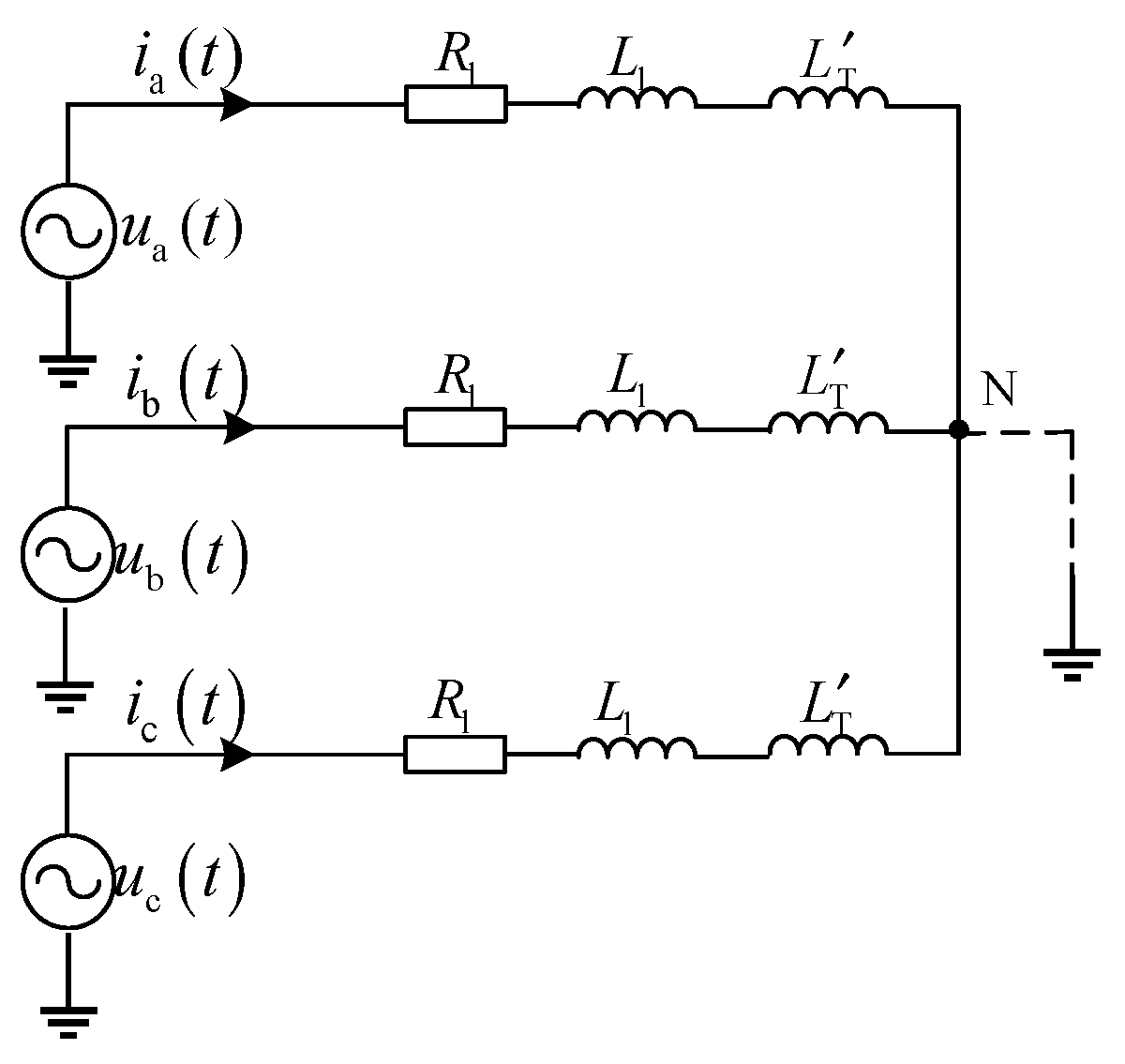
Taking Figure 1 as an example, this paper illustrates the non-fault detection scheme based on DG injection for distribution lines before three-phase reclosing [22]. After the three-phase tripping of the circuit breaker on the power supply side occurs due to a fault in a distribution line, the residual electrical quantities are released after a fixed delay to avoid their impact on subsequent fault state detection results. At the same time, taking advantage of the flexible and controllable characteristics of DG inverters, when disturbance injection is needed into the fault line, the inverter of the DG is used as the disturbance source, and the three-phase symmetrical voltage excitation is applied to the detection feeder within a short time. When the DG cannot implement additional control due to its own operating requirements, an independent disturbance source can be added to the system, if necessary. Using the difference in the characteristics of the circuit response at the point of common coupling (PCC) of the detected line during the excitation period, the fault state is further identified based on the results of model parameter identification. If it is judged to be in a non-fault state, the three-phase reclosing on the line side avoids the risk of blind reclosing failure.

The amplitude and frequency of the three-phase voltage excitation applied by DG are the key parameters of the injection fault detection scheme. Considering that the measurement accuracy of a 10 kV voltage transformer is not less than 5% of the rated voltage $U_{\mathrm{N}}$, the amplitude of the injected voltage $U_{\mathrm{x}}$ should satisfy the relation $U_{\mathrm{x}}\ge 5\%U_{\mathrm{N}}$. At the same time, reference [23] stipulates that the permissible deviation of a supply voltage of 10 kV and below is ±7% of the rated voltage. The range for the amplitude of injected voltage excitation is limited by the relation, i.e., $5\%U_{\mathrm{N}}\le U_{\mathrm{x}}\le 7\%U_{\mathrm{N}}$.

At the same time, the frequency of DG injection voltage excitation should be under the premise of satisfying the inverter’s own working parameters and performance constraints, so that the permanent fault and the instantaneous fault characteristics of arc extinction are significantly different to improve the sensitivity of fault detection [24]. In this paper, the idea of parameter identification is used to identify the time domain method of fault identification [25]. It involves the calculation of the differential substitution derivative of sampling value, which requires a high sampling frequency. Usually, the calculation step size is ${10}^{-4}{~10}^{-5} \mathrm{s}$. In order to reduce the influence of line capacitance and communication and detection results, the frequency of the excitation signal should be selected to be as low as possible; usually its frequency is limited by $10\hspace{0.33em}\mathrm{Hz}\le f_x\le 30\hspace{0.33em}\mathrm{Hz}$ [18].

Admittedly, the necessary communication channel is needed between the detection point and the outlet switch to ensure the implementation of the proposed scheme. With the development of the distribution network construction, the application of a feeder automation system or primary and secondary integration terminal is gradually increasing, and its communication network can provide suitable conditions for the application of fault state identification information transmission.

2.2. Fault Modeling

Taking an AB phase-to-phase fault on the line as an example, this paper conducts a comparative analysis of equivalent networks under transient fault (non-fault) conditions and permanent fault conditions.

2.2.1. Transient Fault (i.e., Non-Fault)

When the distribution line is non-fault or the transient fault has been cleared, its equivalent network is shown in Figure 2. Where $u_{\varphi }(\varphi =\mathrm{a},\mathrm{b},\mathrm{c})$ represents the voltages at the PCC and $i_{\varphi }\left(t\right)$$\left(\varphi =\mathrm{a},\mathrm{b},\mathrm{c}\right)$ is the current in each phase, $R_1$ is the self-resistance of each phase line, $L_1$ is the self-inductance of each phase line, ${L^{\prime }}_{\mathrm{T}}$ is the equivalent inductance of the distribution transformer, and N is the virtual neutral point.

Obviously, when the three-phase symmetrical low-frequency voltage excitation is applied simultaneously by the DG, if the line is in a non-fault state at this time, the three-phase network is symmetrical. The three-phase equivalent network shown in Figure 2 is equivalent to the single-phase equivalent network shown in Figure 3 for analysis.

The equivalent network equations shown in Figure 3 can be obtained as shown in Equation (1):

$$u_{\varphi }\left(t\right)=R_{\mathrm{l}}{i}_{\varphi }\left(t\right)+\left(L_{\mathrm{l}}+{L^{\prime }}_{\mathrm{T}}\right){\displaystyle \frac{d{i}_{\varphi }\left(t\right)}{dt}}=R_{\mathrm{eq}}{i}_{\varphi }\left(t\right)+L_{\mathrm{eq}}{\displaystyle \frac{d{i}_{\varphi }\left(t\right)}{dt}}$$

(1)

From Equation (1), the excitation voltage $u_{\varphi }(t)(\varphi =a,b,c)$ of any phase consists of a linear relationship between $R_{\mathrm{eq}}$ and $L_{\mathrm{eq}}$ of each phase circuit of the line.

2.2.2. Permanent Fault

Similarly, if the phase-to-phase fault still exists when voltage excitation is applied, the line equivalent network is as shown in Figure 4, in which, $R_{\mathrm{f}}$ is the fault transition resistance, m is the distance from the fault point to the head end of the line as a proportion of the total length of the line, and $Z_1$ is the equivalent impedance from the point of failure to the end of the line.

The equivalent network equation illustrated in Figure 4 can be obtained as shown in Equation (2):

$$u_{\mathrm{a}}\left(t\right)=[2m{R}_{\mathrm{l}}+R_{\mathrm{f}}//Z_1]i_{\mathrm{a}}\left(t\right)+2m{L}_{\mathrm{l}}{\displaystyle \frac{d{i}_{\mathrm{a}}\left(t\right)}{dt}}+u_{\mathrm{b}}\left(t\right)$$

(2)

where $Z_1=2(1-m)R_{\mathrm{l}}+2\mathrm{j}\omega (1-m)L_{\mathrm{l}}+2\mathrm{j}\omega {L^{\prime }}_{\mathrm{T}}$.

Obviously, the excitation voltage for any of the faulted phases is related to the fault point location m, the transition resistance $R_{\mathrm{f}}$ and the excitation voltage $u_{\varphi }(t)$ of the other phase, and it cannot be characterized as a linear relationship as shown in Equation (1). For a two-phase ground fault, a similar relationship exists as in Equation (2).

In addition, since a three-phase fault is a symmetrical fault, it can also be analyzed as a single-phase equivalent circuit, and the relationship is shown in Equation (3):

$$u_{\varphi }\left(t\right)=m{R}_{\mathrm{l}}{i}_{\varphi }\left(t\right)+m{L}_{\mathrm{l}}{\displaystyle \frac{d{i}_{\varphi }\left(t\right)}{dt}}$$

(3)

From Equation (3), it can be seen that the excitation voltage $u_{\varphi }\left(t\right)$$\left(\varphi =\mathrm{a},\mathrm{b},\mathrm{c}\right)$ of each phase generated by the DG is related to the resistance $R_{\mathrm{l}}$ and inductance $L_{\mathrm{l}}$ of the line itself from the fault point to the DG access point, i.e., the fault location m is related to the resistance parameter and the inductance parameter in the model, which are significantly different from those in the case of the non-fault condition.

From Equations (1) to (3), it can be seen that there is a significant difference between the non-fault equivalent network and the permanent fault equivalent network, so the difference can be utilized for the screening of the fault state of the three-phase circuit. Based on the principle of model parameter identification, the R–L equivalent network in the non-fault state is used as the reference model, and the voltage and current at the PCC during the excitation period are collected to calculate the equivalent resistance and inductance of the line to be detected; the fault state is identified based on the difference between the recognized values of resistance and inductance and the corresponding actual values.

3. Non-Fault Detection Principle and Criterion Based on R–L Parameter Identification

3.1. Fundamentals

After the exit circuit breaker trips after a fault in the distribution line, the DG simultaneously produces low-frequency voltage excitation to the three phases of the detection line after the fault has disappeared. If the fault has disappeared before applying the excitation, at this time, the excitation voltage at the PCC has a linear relationship with the response current and the response current derivative, and the corresponding expression is as follows:

$$u_{\varphi }\left(t\right)={\widehat{R}}_{\mathrm{eq}}{i}_{\varphi }\left(t\right)+{\widehat{L}}_{\mathrm{eq}}{\displaystyle \frac{d{i}_{\varphi }\left(t\right)}{dt}}$$

(4)

According to the sampling value $(u_{\varphi 1},i_{\varphi 1}),$ $\left(u_{\varphi 2},i_{\varphi 2}\right),\cdots ,\left(u_{\varphi n},i_{\varphi n}\right)$ of the excitation voltage and response current at different times, the matrix expression is obtained as follows:

$$\left[\begin{array}{c}{u}_{\varphi 1}\\ u_{\varphi 2}\\ ⋮\\ u_{\varphi n}\end{array}\right]=\left[\begin{array}{ll}{i}_{\varphi 1}\hfill & {\displaystyle \frac{d{i}_{\varphi 1}}{dt}}\hfill \\ i_{\varphi 2}\hfill & {\displaystyle \frac{d{i}_{\varphi 2}}{dt}}\hfill \\ ⋮\hfill & ⋮\hfill \\ i_{\varphi n}\hfill & {\displaystyle \frac{d{i}_{\varphi n}}{dt}}\hfill \end{array}\right]\left[\begin{array}{c}{\widehat{R}}_{\mathrm{eq}}\\ {\widehat{L}}_{\mathrm{eq}}\end{array}\right]$$

(5)

In this paper, the R–L non-fault equivalent network shown in Figure 3 is used as a calculation model; for the non-fault line, ${\widehat{R}}_{\mathrm{eq}}$ is the line resistance value $R_{\mathrm{l}}$ and ${\widehat{L}}_{\mathrm{eq}}=L_{\mathrm{l}}+{L^{\prime }}_{\mathrm{T}}$, while for the faulty line, the existence of the transition resistance leads to the change of the equivalent circuit: at this time, ${\widehat{R}}_{\mathrm{eq}}$ and ${\widehat{L}}_{\mathrm{eq}}$ are related to the fault location and transition resistance.

In order to calculate ${\widehat{R}}_{\mathrm{eq}}$ and ${\widehat{L}}_{\mathrm{eq}}$, the collected excitation voltages $u_{\varphi }\left(t\right)\left(\varphi =\mathrm{a},\mathrm{b},\mathrm{c}\right)$ and currents $i_{\varphi }\left(t\right)\left(\varphi =\mathrm{a},\mathrm{b},\mathrm{c}\right)$ are fit to linear equations using the least squares method [25], thus obtaining two linear equations, ${\widehat{R}}_{\mathrm{eq}}$ and ${\widehat{L}}_{\mathrm{eq}}$, for solving coefficients. For the presence of faults, there is a significant difference between the identified resistance value of line parameters ${\widehat{R}}_{\mathrm{eq}}$ and the corresponding true resistance $R_{\mathrm{l}}$, and there is a significant difference between the identified inductance value ${\widehat{L}}_{\mathrm{eq}}$ and the corresponding true inductance value. When the parameter identification results are highly consistent with the corresponding true values, that is ${\widehat{R}}_{\mathrm{eq}}=R_{\mathrm{l}}$ and ${\widehat{L}}_{\mathrm{eq}}=L_{\mathrm{l}}+{L^{\prime }}_{\mathrm{T}}$, it indicates that the actual model is consistent with the reference non-fault model, i.e., the line is in non-fault state.

Construct the objective function as follows:

$$F_k^2={{\displaystyle \sum _{k=1}^N\left({\widehat{R}}_{\mathrm{eq}}{i}_{\varphi }\left(k\right)+{\widehat{L}}_{\mathrm{eq}}\frac{d{i}_{\varphi }\left(k\right)}{dt}-u_{\varphi }\left(k\right)\right)}}^2$$

(6)

where $u_{\varphi }\left(k\right)$ is the excitation voltage at the kth sampling point, $i_{\varphi }\left(k\right)$ is the current at the kth sampling point, and N is the number of sampling points.

Take the partial derivatives for ${\widehat{R}}_{\mathrm{eq}}$ and ${\widehat{L}}_{\mathrm{eq}}$ and their extremes, respectively:

$$\left\{\begin{array}{l}{\displaystyle \sum _{k=1}^N\left({\widehat{R}}_{\mathrm{eq}}{i}_{\varphi }\left(k\right)+{\widehat{L}}_{\mathrm{eq}}\frac{d{i}_{\varphi }\left(k\right)}{dt}-u_{\varphi }\left(k\right)\right)i_{\varphi }\left(k\right)=0}\\ {\displaystyle \sum _{k=1}^N\left({\widehat{R}}_{\mathrm{eq}}{i}_{\varphi }\left(k\right)+{\widehat{L}}_{\mathrm{eq}}\frac{d{i}_{\varphi }\left(k\right)}{dt}-u_{\varphi }\left(k\right)\right)\frac{d{i}_{\varphi }\left(k\right)}{dt}=0}\end{array}\right.$$

(7)

Available from above:

$$\left[\begin{array}{c}{\widehat{R}}_{\mathrm{eq}}\\ {\widehat{L}}_{\mathrm{eq}}\end{array}\right]={\left[\begin{array}{cc}{\displaystyle \sum _{k=1}^N{\left(i_{\varphi }\left(j\right)\right)}^2}& {\displaystyle \sum _{k=1}^N\frac{d{i}_{\varphi }\left(j\right)}{dt}{i}_{\varphi }\left(j\right)}\\ {\displaystyle \sum _{k=1}^N\frac{d{i}_{\varphi }\left(j\right)}{dt}{i}_{\varphi }\left(j\right)}& {\displaystyle \sum _{k=1}^N{\left(\frac{d{i}_{\varphi }\left(j\right)}{dt}\right)}^2}\end{array}\right]}^{-1}\left[\begin{array}{c}{\displaystyle \sum _{k=1}^N{u}_{\varphi }\left(j\right)i_{\varphi }\left(j\right)}\\ {\displaystyle \sum _{k=1}^N{u}_{\varphi }\left(j\right)\frac{d{i}_{\varphi }\left(j\right)}{dt}}\end{array}\right]$$

(8)

Using Equation (8), the identification values of the equivalent resistance ${\widehat{R}}_{\mathrm{eq}}$ and equivalent inductance ${\widehat{L}}_{\mathrm{eq}}$ of the line can be obtained.

3.2. Non-Fault Identification Criteria

The fitted evaluation coefficients ${\widehat{R}}_{\mathrm{eq}}$ and ${\widehat{L}}_{\mathrm{eq}}$ obtained through linear fitting using the least squares method can be used to identify the nature of the fault. For a transient fault, the calculated ${\widehat{R}}_{\mathrm{eq}}$ and ${\widehat{L}}_{\mathrm{eq}}$ are equal to the actual values $R_{\mathrm{real}}$ and $L_{\mathrm{real}}$. But for a permanent fault, the calculated values of ${\widehat{R}}_{\mathrm{eq}}$ and ${\widehat{L}}_{\mathrm{eq}}$ are significantly different from the actual values of $R_{\mathrm{real}}$ and $L_{\mathrm{real}}$. Aiming at the difference between ${\widehat{R}}_{\mathrm{eq}}$ and ${\widehat{L}}_{\mathrm{eq}}$ obtained by parameter identification and the actual values $R_{\mathrm{real}}$ and $L_{\mathrm{real}}$, the non-fault identification criterion is proposed as shown in Equation (9):

$$\left\{\begin{array}{c}\Delta R_{\mathrm{th}\text{\_}\varphi }<K_{1\mathrm{rel}}{R}_{\mathrm{real}}=R_{\mathrm{set}}\\ \Delta L_{\mathrm{th}\text{\_}\varphi }<K_{2\mathrm{rel}}{L}_{\mathrm{real}}=L_{\mathrm{set}}\end{array}\right.$$

(9)

where the identification deviation values of resistances and inductances are represented as $\Delta R_{\mathrm{th}\text{\_}\varphi }={\displaystyle \frac{1}{n}}{\displaystyle \sum _{j=1}^n\left|{\widehat{R}}_{\mathrm{eq}}\left(j\right)-R_{\mathrm{real}}\right|}$ and $\Delta L_{\mathrm{th}\text{\_}\varphi }={\displaystyle \frac{1}{n}}{\displaystyle \sum _{j=1}^n\left|{\widehat{L}}_{\mathrm{eq}}\left(j\right)-L_{\mathrm{real}}\right|}$, respectively.

Furthermore, n is the length of the sequence of calculation results, ${\widehat{R}}_{\mathrm{eq}}(j)$ is the least squares calculation of the resistance sequence, ${\widehat{L}}_{\mathrm{eq}}(j)$ is the least squares calculation of the inductance sequence, and $K_{1\mathrm{rel}}$ and $K_{2\mathrm{rel}}$ are the margin coefficients. Due to the influence of model error and algorithm calculation error, the criterion needs to reserve a certain margin. The coefficients $K_{1\mathrm{rel}}$ and $K_{2\mathrm{rel}}$ are set from 0.1 to 0.2, which can meet the requirements of fault nature discrimination. When the two conditions of Equation (9) are met, it can be judged as a non-fault state (i.e., an instantaneous fault with arc extinction). Otherwise, it is judged as a persistent state fault, i.e., a permanent fault.

3.3. Realizing Scheme

The implementation of the active distribution network phase-to-phase fault state identification proposed in this paper is shown in Figure 5.

Step 1: In order to avoid the influence of residual electrical quantities in the fault line on the discrimination results after the three-phase trip of the distribution line fault, a low-frequency voltage excitation is applied to the three phases of the tested line by DG after the breaker trips with a 50–100 ms delay.

Step 2: Collect voltage $u_{\varphi }(t)(\varphi =\mathrm{a},\mathrm{b},\mathrm{c})$ and current $i_{\varphi }(t)(\varphi =\mathrm{a},\mathrm{b},\mathrm{c})$ data at PCC, then sequentially solve the three-phase resistance and inductance parameter identification values using Equation (8).

Step 3: If the criterion shown in Equation (9) is satisfied, it is determined as a non-fault state (indicating the arc extinction state of a transient fault), and the circuit breaker will issue a reclosing command. If the criterion remains unsatisfied until the maximum discrimination time is reached, it is determined that the inter-phase loop still contains a fault (i.e., considered as permanent fault), and the reclosing operation will be blocked. When the maximum allowed discrimination time is not yet reached, the process returns to step (2) for iterative determination.

4. Simulation Experiment Based on PSCAD

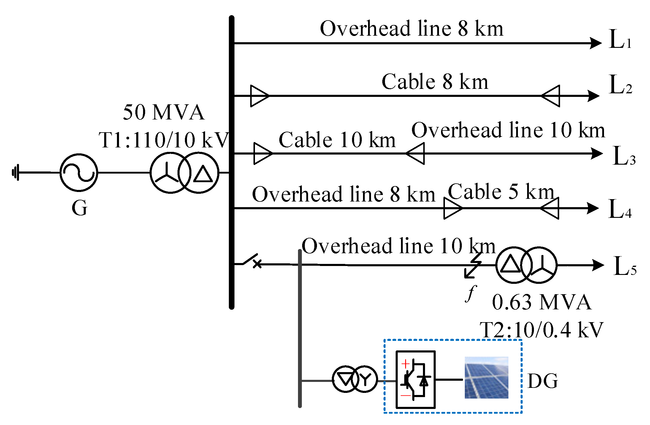
4.1. Simulation Model

The 10 kV distribution network model is constructed using PSCAD/EMTDC as shown in Figure 6.

As shown in Figure 6, lines L₁ and L₅ are overhead lines with lengths of 8 km and 10 km, respectively. L₂ is a pure cable line with a length of 8 km; L₃ and L₄ adopt an overhead-cable hybrid structure, where L₃ consists of a 10 km cable section and a 10 km overhead section and L₄ consists of an 8 km cable section and a 5 km overhead section. The distribution line per-unit parameters are shown in

Table 1. Distribution per-unit parameters.

Line Type	Phase Sequence	Resistance (Ω/km)	Inductance (mH/km)	Capacitance (μF/km)
overhead line	positive sequence	0.125	1.299	0.040
	zero sequence	0.275	4.586	0.012
cable line	positive sequence	0.270	0.254	0.339
	zero sequence	2.700	1.019	0.280

.

4.2. Simulation Calculations

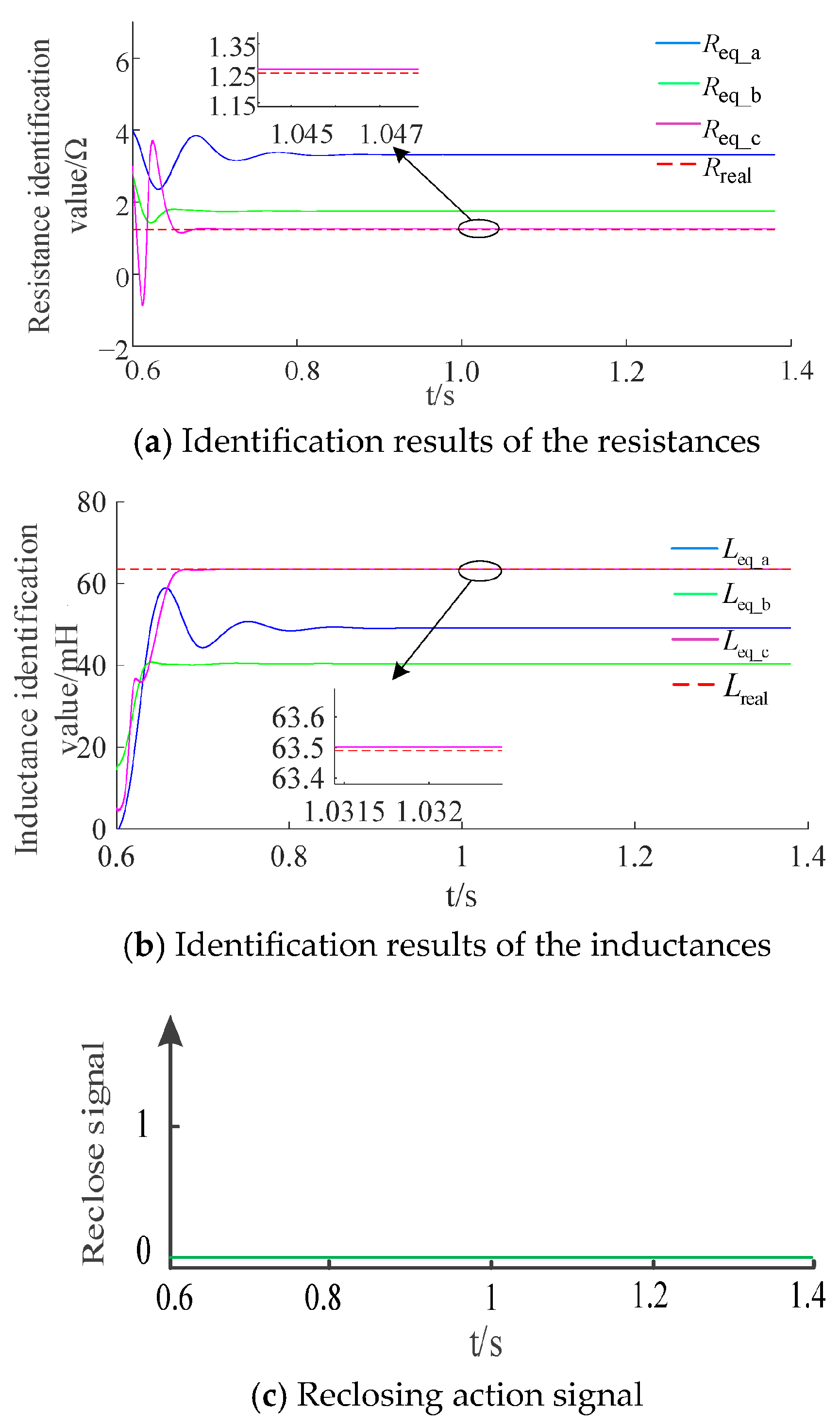
4.2.1. Identification Criterion Principles Verification

It is assumed that the AB phase-to-phase fault with a transition resistance of 10 Ω occurs at the midpoint of the line L₅. The fault occurs in 0.3 s, the three-phase tripping of the outlet circuit breaker in 0.32 s, and the voltage of 20 V/10 Hz is applied to the three phases of the line L₅ to be detected at the same time by the DG in 0.6 s. The voltage excitation of 500 V/10 Hz can be obtained using the step-up transformer. The transient fault lasts for 0.7 s, and the permanent fault lasts until the end of the simulation. The sampling frequency is 10 kHz, and the length of the calculation data window is 20 ms; that is, 200 sampling data points are used to calculate a set comprising resistance and inductance data.

The actual values of resistance and inductance of each phase of the corresponding non-fault circuit are calculated as follows:

$$\left\{\begin{array}{l}{R}_{\mathrm{real}}=R_{\mathrm{L}1}\times 10=1.25\hspace{0.17em}\Omega \\ L_{\mathrm{real}}=L_{\mathrm{L}1}\times 10+{L^{\prime }}_{\mathrm{T}}=L_{\mathrm{L}1}+L_{{\mathrm{T}}^{\ast }}{\displaystyle \frac{{U_{\mathrm{T}1}}^2}{{\omega }_1{S}_{\mathrm{T}}}}=63.49 \mathrm{mH}\end{array}\right.$$

(10)

where $R_{\mathrm{L}1}$ is the positive sequence resistance of the line, $L_{\mathrm{L}1}$ is the positive sequence inductance of the line, $L_{{\mathrm{T}}^{\ast }}$ is the nominal value of the distribution transformer, $U_{\mathrm{T}1}$ is the rated voltage of the primary side of the distribution transformer, $S_{\mathrm{T}}$ is the rated capacity of the distribution transformer, and ${\omega }_1$ is the angular frequency at the industrial frequency.

After calculating the actual values of resistance and inductance, the threshold value of the criterion can be further calculated. The reliability coefficients $K_{1\mathrm{rel}}$ and $K_{2\mathrm{rel}}$ are 0.2. According to Equation (9), the action threshold corresponding to the criterion is

$$\left\{\begin{array}{l}\Delta R_{\mathrm{th}\text{\_}\varphi }<R_{\mathrm{set}},R_{\mathrm{set}}=K_{1\mathrm{rel}}{R}_{\mathrm{real}}=0.25 \Omega \\ \Delta L_{\mathrm{th}\text{\_}\varphi }<L_{\mathrm{set}},L_{\mathrm{set}}=K_{2\mathrm{rel}}{L}_{\mathrm{real}}=12.69 \mathrm{mH}\end{array}\right.$$

(11)

When both the identified resistance and inductance values satisfy the relationship defined in Equation (11), it is reliably judged as a non-fault condition. When at least one parameter (resistance or inductance) fails to satisfy Equation (11), it indicates the existence of an permanent inter-phase fault on the line.

To demonstrate the effectiveness of the proposed discrimination method, Figure 7 and Figure 8 present the identification results of the three-phase resistance and inductance parameters for line L₅ under AB phase-to-phase permanent fault and transient fault conditions.

As can be seen from the results shown in Figure 7a,b, when a permanent fault occurs, the actual fault model is inconsistent with the recognition model, and the corresponding resistance and inductance recognition values are significantly different from the actual resistance and inductance parameters, of which the three-phase resistance parameter recognition deviations are $\Delta R_{\mathrm{th}\text{\_}\mathrm{a}}$ = 1.654 Ω, $\Delta R_{\mathrm{th}\text{\_}\mathrm{b}}$ = 0.400 Ω, and $\Delta R_{\mathrm{th}\text{\_}\mathrm{c}}$ = 0.010 Ω respectively. Moreover, the three-phase inductance parameter recognition deviations are $\Delta L_{\mathrm{th}\text{\_}\mathrm{a}}$ = 13.7 mH, $\Delta L_{\mathrm{th}\text{\_}\mathrm{b}}$ = 23.4 mH, and $\Delta L_{\mathrm{th}\text{\_}\mathrm{c}}$ = 0.010 mH, respectively, which means that the relationship between the three-phase resistance and inductance identification results and the corresponding real values has at least one item that does not satisfy the relationship shown in Equation (11), which indicates that the fault is on the line L₅ and the arc has not been extinguished. As illustrated in Figure 7c, the system protection logic persistently blocks the reclosing operation due to the real-time identified parameters of line resistance and inductance failing to satisfy the criteria defined in Equation (11) (at least one parameter exceeds the threshold). Consequently, the actuation signal remains at a zero-level state.

Figure 8 shows the results of a transient fault. Seen from Figure 8a,b before the fault disappears at 1.0 s, the actual fault model and the identification model are inconsistent. Significant discrepancies exist between the identified resistance, inductance values and the corresponding actual values, and the exhibited characteristics are similar to those of permanent faults described above. Seen from Figure 8c, in the stage before the fault arc extinguishing time t = 1.1 s, the identification results of the resistance or inductance parameters of each phase circuit of the line to be detected do not meet the relationship shown in Equation (11); that is, the fault state is judged, and the reclosing of the corresponding outlet switch is locked, i.e., the low-level signal is generated.

In Figure 8a,b, after the fault disappears at 1.0 s, the actual fault model aligns with the identification model. The identified resistance and inductance parameters match the actual parameters, with maximum deviations of $\Delta R_{\mathrm{th}\text{\_}\mathrm{a}}$ = 0.013 Ω for resistance and $\Delta L_{\mathrm{th}\text{\_}\mathrm{a}}=0.010\hspace{0.33em}\mathrm{mH}$ for inductance. During this phase, the relationship between the three-phase resistance or inductance identification results of line L₅ and their true values consistently satisfies the relationship defined in Equation (11). In Figure 8c, at t = 1.1 s, the identification results of the resistance and inductance values of each phase loop of the line to be detected are in accordance with the relationship shown in Equation (11); that is, the line is judged to be in a non-fault state, and the corresponding reclosure of the outlet circuit breaker is in an open state and triggers the high-level signal for closing. Thus, line L₅ is reliably judged to be in a non-fault state.

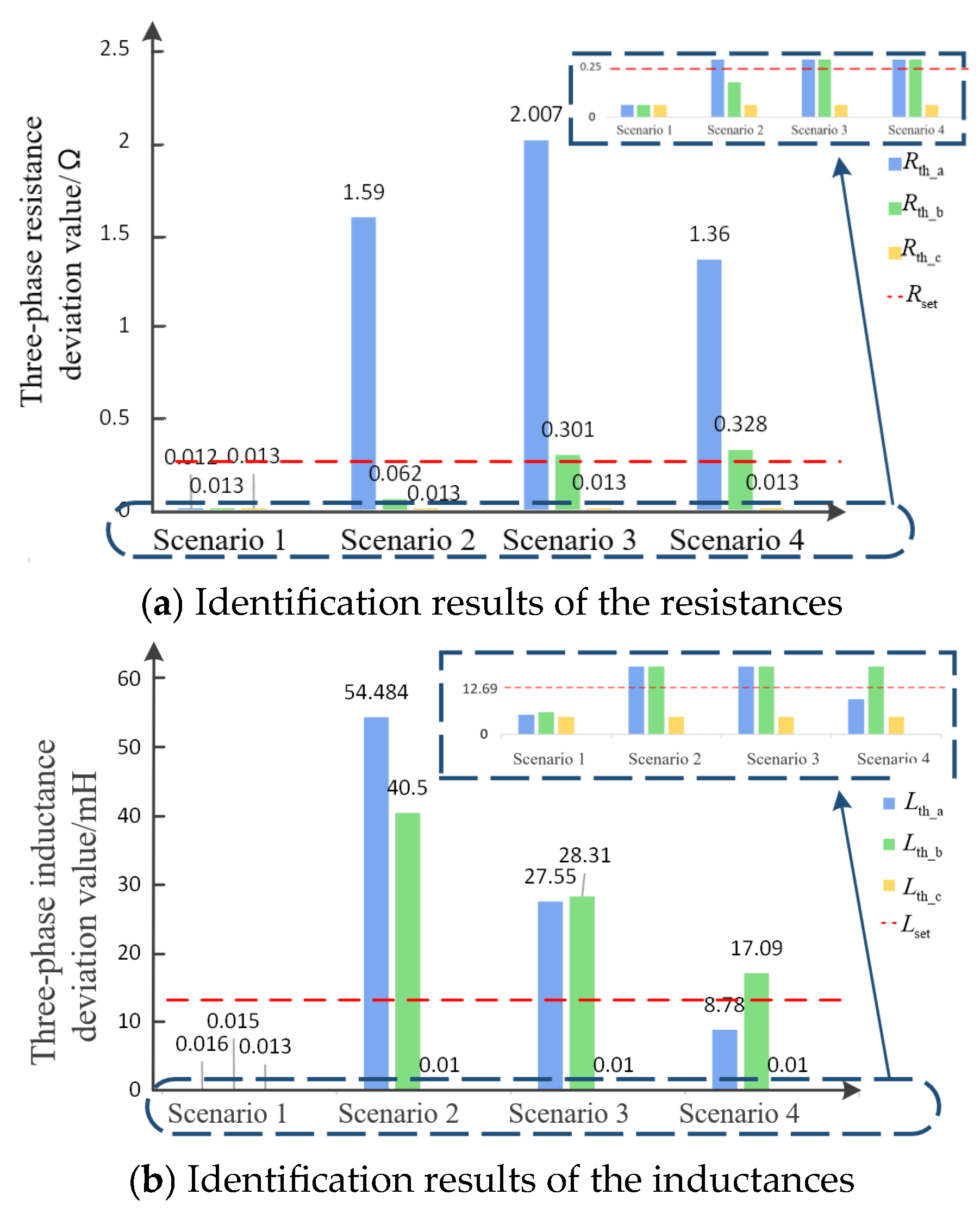
4.2.2. Performance Analysis Under Different Fault Conditions

In order to verify the applicability of the proposed method in the first section and the end of the line, this paper designs the following four scenarios according to different transition resistances. The calculation results of AB phase-to-phase faults under different conditions of the line L₅ are shown in Figure 9 and Figure 10.

• Scenario 1: Transient fault occurs with 1 Ω transition resistance.
• Scenario 2: Permanent fault occurs with 5 Ω transition resistance.
• Scenario 3: Permanent fault occurs with 10 Ω transition resistance.
• Scenario 4: Permanent fault occurs with 20 Ω transition resistance.

Next, simulation calculations are carried out separately for the four fault scenarios mentioned above at the beginning and end of the line. The result of AB phase-to-phase short circuit at the head of the line (m = 0.1) and at the end of the line (m = 0.9) are shown in Figure 10.

The results of an AB phase-to-phase short circuit at the beginning of the line are shown in Figure 9.

In Scenario 1, both the resistance and inductance deviations are smaller than the threshold values, so the line is judged as non-fault. And in scenarios 2–4, even with a transition resistance of 20 Ω (the transition resistance for phase-to-phase faults generally does not exceed 20 Ω), the deviations of the three-phase resistance identification values ($R_{\mathrm{eq}\text{\_}\mathrm{a}}$ = 1.36 Ω and $R_{\mathrm{eq}\text{\_}\mathrm{b}}$ = 0.328 Ω) differ from the actual resistance value $R_{\mathrm{real}}$ = 0.25 Ω. Additionally, the identified inductance value $L_{\mathrm{eq}\text{\_}\mathrm{b}}$ = 17.09 mH significantly deviates from the actual inductance value $L_{\mathrm{real}}$ = 12.69 mH. These discrepancies violate the relationship defined in Equation (11), failing to meet the non-fault criteria, and are thus identified as permanent faults.

The results of an AB phase-to-phase short circuit at the end of the line are shown in Figure 10. In Scenario 1, the differences between the calculated values and actual values of both resistance and inductance satisfy Equation (11); thus it is judged as a non-fault condition. In scenarios 2–3, even with a transition resistance of 20 Ω (the transition resistance for phase-to-phase faults generally does not exceed 20 Ω), there remains significant discrepancy between the calculated resistance values ($R_{\mathrm{eq}\text{\_}\mathrm{a}}$ = 0.961 Ω and $R_{\mathrm{eq}\text{\_}\mathrm{b}}$ = 0.53 Ω) and the actual resistance value ($R_{\mathrm{real}}$ = 0.25 Ω). In these cases, at least one parameter (either the actual resistance $R_{\mathrm{real}}$ or actual inductance $L_{\mathrm{real}}$) shows significant deviation, failing to satisfy the non-fault criteria. Therefore, the criteria proposed in this paper can reliably identify inter-phase permanent faults.

In addition, in order to more fully illustrate the effectiveness of the proposed method, the sample size of the fault simulation scenario is expanded to 120 groups, of which 80% are transient faults. By setting different fault types, the stability of the fault identification method is systematically tested. It has absolute reliability for the identification of the fault-free state of the arc extinction and ensures that the three phases do not coincide with the fault state of the non-extinguishing arc.

At the same time, due to the limitation of the existing experimental conditions, it is difficult to carry out the simulation test of introducing the additional disturbance control of the real inverter for fault detection. In terms of the need to enhance the credibility of the application of the proposed scheme in the future, it is necessary to further strengthen the research and experimental work.

5. Comparison with Other Methods

To validate the superiority of the proposed method, voltage deviation analysis is designed based on the aforementioned four scenarios. During non-fault disturbance conditions, ignoring the line impedance and transformer impedance, the voltage difference $\Delta U_{\varphi }(\varphi =\mathrm{a},\mathrm{b},\mathrm{c})$ between the PCC voltage ($U_{\mathrm{PCC}}$) and the injection source voltage referred to the high-voltage side ($U_{\mathrm{G}}$) is zero. When a phase-to-phase fault occurs, an inter-phase loop forms with fault current circulation, causing elevation of $U_{\mathrm{PCC}}$. In this case, significant deviation emerges in the voltage difference $\Delta U_{\varphi }(\varphi =\mathrm{a},\mathrm{b},\mathrm{c})$ between $U_{\mathrm{PCC}}$ and $U_{\mathrm{G}}$. Considering the transformer impedance voltage drop, system modeling errors and voltage transformer measurement accuracy, the discrimination criterion can be established as follows:

$$\Delta U_{\varphi }<K_{\mathrm{rel}}\Delta U_{\mathrm{T}}(\varphi =\mathrm{a},\mathrm{b},\mathrm{c})$$

(12)

In this paper, the transformer impedance voltage drop $\Delta U_{\mathrm{T}}$ is set to 1~2% of the source voltage. Additionally, the discrimination criterion requires a safety margin, where $K_{\mathrm{rel}}$ ranging from 1 to 3 meets the requirements for fault type identification. Therefore, $\Delta U_{\mathrm{set}}=K_{\mathrm{rel}}\Delta U_{\mathrm{T}}$$<2\times 2\%\times 500\begin{array}{c}\end{array}\mathrm{V}=20\begin{array}{c}\end{array}\mathrm{V}$.

When the line voltage deviation satisfies Equation (12), the condition is determined as non-fault. Conversely, failure to meet Equation (12) indicates the occurrence of a phase-to-phase fault on the line.

Figure 11 shows the voltage deviations during an AB phase-to-phase fault at the sending terminal of the line. In Scenario 1, both voltage deviations of phases A and B $\Delta U_{\mathrm{a}}=15.200\begin{array}{c}\end{array}\mathrm{V}$ and $\Delta U_{\mathrm{b}}=15.199\begin{array}{c}\end{array}\mathrm{V}$ satisfy the criterion shown in Equation (12), leading to a non-fault determination. In scenarios 2–3, the voltage deviations of faulted phases AB exceed the threshold, resulting in permanent fault identification.

To compare the sensitivity of both methods, the sensitivity coefficients for the aforementioned criteria are calculated using Equation (13), where $R_{\mathrm{eq}\text{\_}\varphi }$, $L_{\mathrm{eq}\text{\_}\varphi }$ and $U_{\mathrm{PCC}\text{\_}\varphi }$ all adopt the maximum values in each phase. The calculation results for the four predefined scenarios are summarized in

Table 2. Sensitivity coefficient.

Scenario	${\mathit{K}}_{\mathbf{R}}$	${\mathit{K}}_{\mathbf{L}}$	${\mathit{K}}_{\mathbf{U}}$
Scenario 1	0.0072	0.0003	0.0310
Scenario 2	1.2720	0.6379	0.1930
Scenario 3	1.6056	0.4339	0.1252
Scenario 4	1.0880	0.26918	0.1184

.

$$\left\{\begin{array}{l}{K}_{\mathrm{R}}={\displaystyle \frac{\left|R_{\mathrm{real}}-R_{\mathrm{eq}\text{\_}\varphi }\right|}{R_{\mathrm{real}}}}\\ K_{\mathrm{L}}={\displaystyle \frac{\left|L_{\mathrm{real}}-L_{\mathrm{eq}\text{\_}\varphi }\right|}{L_{\mathrm{real}}}}\\ K_{\mathrm{U}}={\displaystyle \frac{\left|U_{\mathrm{G}}-U_{\mathrm{PCC}\text{\_}\varphi }\right|}{U_{\mathrm{G}}}}\end{array}\right.$$

(13)

The sensitivity comparison of both methods for an AB phase-to-phase fault at the sending terminal of the line is presented in Table 2. Although the inductance sensitivity drops below 0.5 after fault occurrence, the resistance sensitivity consistently remains above 0.5. The proposed method only requires either resistance or inductance sensitivity to meet the 0.5 threshold for reliable fault discrimination. Voltage sensitivity remains below 0.5 across all test scenarios in this study, confirming the superior sensitivity of the proposed method.

Furthermore, to validate the adaptability of the proposed scheme, extensive simulation studies verify that the method reliably discriminates pre-reclosing fault conditions: it enables successful reclosing when non-fault status is identified and securely blocks reclosing for permanent faults. This effectively mitigates the risk of secondary impacts caused by blind reclosing on permanent faults.

6. Discussion

In the process of analysis, this paper simplifies the design of the additional control strategy of the distributed power supply itself. The special design of the control strategy of the inverter is the key to the implementation of the disturbance injection fault detection scheme. Only by the analysis of the principle of the proposed disturbance-based fault state detection, can the specific implementation strategy of additional control meet the requirements of the existing research work. In the process of theoretical analysis and criterion construction, only the access scenario of a single DG is considered. In fact, there are multiple DG access scenarios in the feeder. The implementation of the disturbance and the coordination relationship between DGs are also practical problems that determine whether they can be applied in engineering. However, based on the requirements of the future engineering application of this method, it is highly necessary to carry out in-depth research on the strategy of implementing disturbance fault detection in combination with the actual inverter module of DG.

In addition, in the process of theoretical analysis and criterion construction, only the access scenario of a single DG is considered. In fact, there are multiple DG access scenarios in the feeder, and its disturbance implementation method and the coordination relationship between DGs at different locations are also practical problems that affect engineering applications. Subsequently, the optimization scheme of disturbance implementation in multiple DG access scenarios, the disturbance coupling response characteristics between different DGs and the coordinated control strategy of fault detection between different DGs will be further studied.

It should be pointed out that the verification of the method proposed in this paper is currently being carried out through strict electromagnetic transient simulation based on PSCAD/EMTDC. Because it can realize the digital simulation of complex fault scenarios in a distributed power distribution network with high precision, it has been widely used in the research of power systems, and can provide effective test support for the principle and scheme verification of disturbance fault detection in this paper. Obviously, the simulation test of the corresponding disturbance additional control strategy combined with the real photovoltaic inverter can confirm the feasibility of the disturbance injection detection scheme in this paper, but the experimental conditions such as the hardware module of the photovoltaic inverter and the simulation physics of the distribution network line need to be established. It is highly regrettable that the current research team does not have the working conditions in which to carry out the above tests. In the future, we will further strengthen the construction of real experimental test conditions and continuously improve the performance of the developed non-fault detection scheme.

7. Conclusions

This paper studied a three-phase reclosing fault state detection method for a distribution network with DG. Taking full advantage of the flexible and controllable characteristics of power electronic links such as distributed power inverters, the response characteristics of the detection circuit with temporary low-frequency voltage excitation on the line to be tested are used to further obtain the equivalent resistance and inductance parameters of the detection circuit, so as to perceive the difference of the circuit state. Finally, a three-phase reclosing fault-free state identification scheme is formed. The key findings are summarized as follows:

(1) During the fault state detection using the distributed power disturbance response, there is a significant difference between the phase-to-ground circuit when the fault lasts and the phase-to-ground circuit when the fault disappears (i.e., the arc is extinguished); that is, the electrical relationship between the equivalent resistance and inductance parameters represented by the corresponding phase circuits is inconsistent.

(2) In addition, the fault-free R–L equivalent network is used as the identification model, which is not limited by factors such as fault location and transition resistance. The fault-free state is identified by the difference between the identified value and the actual value of the resistance and inductance during the disturbance of the line-side DG. The physical meaning is clear and intuitive, the threshold is easy to set, and the fault-free identification criterion is simple.

(3) Furthermore, the proposed scheme is based on the additional disturbance control strategy of the DG inverter without disconnection of the line to be detected. Under the premise of ensuring that the safety of system operation is not affected, some DGs are selected according to the requirements to temporarily apply a specific low-frequency voltage excitation for fault state detection. For feeders with a large number of distributed power access points, there is no need to configure additional disturbance devices for fault detection, which has good economic and application prospects.

References

1. Si, R.; Yan, X.; Liu, W.; Zhang, P.; Wang, M.; Li, F.; Yang, J.; Su, X. Hybrid optimization-based sequential placement of DES in unbalanced active distribution networks considering multi-scenario operation. Energies 2025, 18, 474. [Google Scholar] [CrossRef]
2. Ma, X.; Zhen, W.; Ren, H.; Zhang, G.; Zhang, K.; Dong, H. A method for fault localization in distribution networks with high proportions of distributed generation based on graph convolutional networks. Energies 2024, 17, 5758. [Google Scholar] [CrossRef]
3. Ayanlade, S.O.; Ariyo, F.K.; Jimoh, A.; Akindeji, K.T.; Adetunji, A.O.; Ogunwole, E.I.; Owolabi, D.E. Optimal Allocation of photovoltaic distributed geberation in radial distribution networks. Sustainability 2023, 15, 13933–13956. [Google Scholar]
4. Gao, W.L.; Xi, M.D.; Wang, H. New method of small current grounding line selection based on feature fusion and extreme learning machine. Electron. Meas. Technol. 2023, 46, 176–184. [Google Scholar]
5. Zhao, J.W.; Zhang, H.B.; Hu, Y.J. Adaptive distance protection for distributed generation distribution network with T-connected inverter interfaced distributed generation. Renew. Energy Resour. 2024, 42, 64–70. [Google Scholar]
6. Sao, W.Q.; Liu, Y.; Zhang, Z.H. Non-Fault detection for three-phase reclosing in transmission lines based on calculated differential-currents. Power Syst. Clean Energy 2017, 33, 18–23. [Google Scholar]
7. Cao, H.; Xia, Q.; Yu, B. Intelligent reclosing strategy for near area AC transmission lines connected with UHVDC. Power Syst. Prot. Control 2022, 50, 156–163. [Google Scholar]
8. Shen, J.; Shu, Z.S.; Chen, J. Application of adaptive auto-reclosure in power system. Autom. Electr. Power Syst. 2018, 42, 152–156. [Google Scholar]
9. Khan, W.A.; Tianshu, B.I.; Ke, J. A review of single phase adaptive auto-reclosing schemes for EHV transmission lines. Prot. Control Mod. Power Syst. 2019, 4, 205–214. [Google Scholar]
10. Deb, S.; Lata, S.; Bhadoria, V.S. Improved Relay Algorithm for Detection and Classification of Transmission Line Faults in Monopolar HVDC Transmission System Using Signum Function of Transient Energy. IEEE Access 2024, 12, 15561–15571. [Google Scholar]
11. Li, C.L.; Ma, C.; Wang, C.Y. Study on relay protection of distribution network containing distributed generation based on adaptive algorithm. Renew. Energy Resour. 2015, 33, 1329–1339. [Google Scholar]
12. Zhang, Z.H.; Qiao, H.; Shao, W.Q. Non-fault detection in phase-to-phase faults before reclosing in distribution network. Grid Anal. Study 2018, 46, 66–71. [Google Scholar]
13. Liao, H.Y.; Kang, X.N.; Yuan, Y.L. Adaptive three-phase reclosing device of distribution network based on injected signals. Power Syst. Technol. 2021, 45, 2623–2630. [Google Scholar]
14. Song, M.M.; Liu, J.; Zhang, Z.H. Power quality analysis based on power consumption information acquisition data. Distrib. Util. 2020, 37, 51–57. [Google Scholar]
15. Shao, W.Q.; Liu, Y.X.; Guan, X. An active detection scheme for permanent fault identification before phase-to-phase reclosing in a distribution network. Power Syst. Prot. Control 2021, 49, 96–103. [Google Scholar]
16. Shao, W.Q.; He, Y.X.; Guan, X. Identification method for an interphase permanent fault in a distribution network using waveform characteristics of multiple disturbance currents. Power Syst. Prot. Control 2023, 51, 146–157. [Google Scholar]
17. Zu, K.; Song, Y.T.; Xu, Y.G. An active adaptive reclosing scheme for distribution lines. Power System Technology 2017, 41, 993–999. [Google Scholar]
18. Zhuo, J.; Shao, W.Q.; Guan, X. Permanent fault identification method of distribution network based on parameter identification. Distrib. Energy 2022, 7, 37–45. [Google Scholar]
19. Zhang, Z.H.; Liu, J.; Ren, B.J. Permanent fault identification for distribution network based on characteristic frequency signal injection using power electronic technology. Front. Energy Res. 2022, 10, 967592. [Google Scholar] [CrossRef]
20. Jiao, Z.B.; Ma, T.; Qu, Y.J. A novel excitation inductance-based power transformer protection scheme. Proc. CSEE 2014, 34, 1658–1666. [Google Scholar]
21. Huang, Z.H.; Zou, J.Y.; Zou, Q.T. Research on controlled reclosing for solidly earthed neutral systems. Proc. CSEE 2016, 36, 4753–4762. [Google Scholar]
22. Meng, H.D.C.F.; Zhao, L. Fault identification technology for distribution line based on distributed generation injection signal. High Volt. Appar. 2022, 58, 123–129+146. [Google Scholar]
23. GB/T 12325-2008; Power Quality—Deviation of Supply Voltage. Standards Press of China: Beijing, China, 2008.
24. Xu, R.D.; Chang, Z.X.; Song, G.B. Grounding fault identification method for DC distribution network based on detection signal injection. Power Syst. Technol. 2021, 45, 4269–4277. [Google Scholar]
25. Lin, J.Y.; Chen, R.; Li, Y.L. Fault Location Method for Distribution Network Based on Parameter Identification. South. Power Syst. Technol. 2019, 13, 80–87. [Google Scholar]
Figure 1. Fault detection system based on injection by DG into an active distribution network.
Energies 18 01932 g001
Figure 2. Non-fault equivalent network of a distribution network.
Energies 18 01932 g002
Figure 3. Non-fault equivalent network diagram.
Energies 18 01932 g003
Figure 4. Distribution line AB permanent fault equivalent network.
Energies 18 01932 g004
Figure 5. Realizing scheme.
Energies 18 01932 g005
Figure 6. 10 kV distribution network model.
Energies 18 01932 g006
Figure 7. Results for a permanent fault.
Energies 18 01932 g007
Figure 8. Results of transient fault.
Energies 18 01932 g008
Figure 9. Results of the faults occurring at the beginning of the line (m = 0.1).
Energies 18 01932 g009
Figure 10. Results of the faults occurring at the end of the line (m = 0.9).
Energies 18 01932 g010
Figure 11. Results of criterion using voltage deviation.
Energies 18 01932 g011