A Two-Stage Hidden Markov Model for Medium- to Long-Term Multiple Wind Farm Power Scenario Generation

Abstract

Medium- to long-term wind power output scenarios are crucial for power system planning and operational simulations. This paper proposes a two-stage hidden Markov model-based approach for modeling the time series output of multiple wind farms. First, based on the key features of the wind power output sequence, the daily typical patterns of wind power output are extracted. Then, the process of simulating the wind power output time-series is modeled as a two-layer temporal model. The upper layer uses a discrete hidden Markov model to describe the day-to-day transition process of wind power output patterns and the lower layer uses a Gaussian mixture hidden Markov model to describe the fluctuation process of wind power output values within each output pattern. Finally, the upper models corresponding to each quarter and the lower models corresponding to each pattern are trained respectively and the time-series scenarios of wind power output for multiple wind farms are generated quarter-by-quarter and day-by-day through Monte Carlo sampling. Validation using real-world wind power data demonstrates that the proposed method can effectively generate medium- to long-term output scenarios for multiple wind farms. Compared to traditional methods, the proposed method shows improvements in terms of accuracy, statistical characteristics, temporal correlation, and mutual correlation.

1. Introduction

The integration of large-scale wind power into modern power systems presents significant operational challenges due to its inherent variability and uncertainty. Wind power generation is influenced by multiple stochastic factors, including wind speed, direction, atmospheric conditions, and complex terrain effects, making it particularly challenging to predict and manage [1]. Traditional deterministic forecasting approaches, which rely on single-point predictions of wind power output, have proven inadequate for the optimization and uncertainty management of advanced power systems with high wind power penetration [2]. The scenario analysis method in stochastic programming theory is one of the effective tools for capturing wind power uncertainty [3,4]. This approach generates multiple scenarios of wind power output sequences that preserve the essential statistical properties and temporal dynamics of historical patterns. By incorporating these scenarios into power system planning and operations, system operators can develop more robust and flexible strategies that explicitly account for wind power uncertainty. This framework enables enhanced economic efficiency and operational reliability in modern power systems.

According to the time scale, wind power output sequence scenarios can be categorized into three temporal scales: ultra-short-term, short-term, and medium-to-long-term scenarios. Among these, medium-to-long-term scenarios play a crucial role in power system planning, capacity expansion, and long-range power balance optimization [5,6]. The inherent chaos in atmospheric dynamics presents fundamental limitations for medium-to-long-term predictions while short-term scenario generation can effectively leverage wind power forecasting and numerical weather prediction (NWP) models. This challenge is compounded by the nonlinear interactions between multiple meteorological variables and their impact on wind power generation. Consequently, the focus in medium-to-long-term scenario generation shifts from achieving precise point-wise predictions to accurately capturing and reproducing the essential statistical characteristics, including temporal fluctuation patterns, spatial correlations among wind farms, and seasonal variations observed in historical data.

Existing approaches to wind power scenario generation can primarily be divided into two methodological frameworks: statistical methods and deep learning techniques. Statistical methods typically employ probabilistic models to characterize the stochastic process of wind power output. Traditional time series approaches, such as the autoregressive moving average (ARMA) model [7,8], have been applied to capture temporal dependencies in wind power output sequences. More sophisticated approaches utilize Markov chain Monte Carlo (MCMC) methods [9,10] to model state transitions and generate scenarios through sequential sampling. Copula theory has been employed [11,12,13] to model the complex correlation among multiple wind farms, enabling the generation of spatial scenarios through multivariate sampling techniques. However, these statistical methods, while mathematically tractable, often struggle to capture the multiscale characteristics of wind power output, particularly the interaction between different temporal scales and spatial dependencies. In recent years, generative models in deep learning methods have been widely applied in the field of scenario generation, mainly including variational autoencoders (VAE) [14,15], generative adversarial networks (GAN) [16,17,18], and normalizing flows (NF) [19,20].

Reference [14] employed an improved VAE to describe the uncertainty of photovoltaic power output and applied the generated scenarios to centralized photovoltaic optimization configuration in multi-energy power systems. However, VAE may introduce reconstruction errors when processing complex wind power data, which limits the accuracy of the generated scenarios. Reference [15] combined VAE with a bidirectional long short-term memory (Bi-LSTM) network to propose a deep learning framework for large-scale renewable energy demand prediction. Although this method improves the capture of time-series features, the limited ability of Bi-LSTM to model long-term dependencies may result in reduced accuracy in long-term wind power forecasts. Reference [16] adopted a GAN for model-free renewable energy scenario generation. However, the training process of GAN is prone to mode collapse, which restricts the diversity of generated wind power scenarios and compromises the comprehensiveness of predictions. Reference [17] proposed a controllable GAN model that allows manual control over the characteristics of generated scenarios. Although this method enhances the controllability of the generated scenarios, the introduction of additional control variables may increase model complexity and training difficulty, thereby impacting the feasibility of practical applications. Reference [18] employed a style-based generative adversarial network and a sequence encoder to generate day-ahead renewable energy output scenarios through the hierarchical control and blending of scene styles. However, the application of Style-GAN in wind power prediction may be constrained by the quality and quantity of samples, resulting in insufficient representativeness of the generated scenarios. Refs. [19,20] indicated that, compared to VAE and GAN, the NF model is more suitable for power system time-series scenario generation. However, NF may face challenges such as high computational complexity and training difficulties when dealing with high-dimensional complex data, limiting its application in large-scale wind power scenario prediction. In summary, existing deep learning methods cannot fully explain the relationship between their model structures and wind power uncertainty, and the model training process is rather cumbersome.

This paper presents a novel methodology for generating medium- to long-term output sequence scenarios across multiple wind farms, with particular attention to both daily pattern variations and intraday output fluctuations. The proposed approach employs a hierarchical framework integrating multiple advanced statistical techniques. First, based on historical data, a feature vector for daily wind power output is constructed. Principal component analysis (PCA) is applied to dimensionality reduction. These reduced-dimension features are then categorized into distinct output patterns using K-means clustering. Secondly, a two-layer temporal modeling framework of multiple wind farms’ output is established. The upper layer implements a discrete hidden Markov model (HMM) to capture transitions between typical daily output patterns, while the lower layer utilizes a Gaussian mixture model–hidden Markov model (GMM–HMM) to characterize intraday output fluctuations within each pattern. Finally, Monte Carlo sampling is employed to simulate and generate sequences of typical output patterns and their corresponding output values, which are subsequently concatenated chronologically to create comprehensive medium- to long-term output sequence scenarios for multiple wind farms while preserving interfarm correlations. The methodology’s efficacy is validated using historical data from two wind farms in southern China, demonstrating robust performance in capturing both temporal dependencies and spatial correlations in wind power generation patterns.

2. Definition of Typical Output Patterns

2.1. Establishment of Daily Wind Power Output Feature Vectors

Wind power generation is influenced by a complex interplay of natural and operational factors, including wind speed, wind direction, air density, wind turbine operational status, and grid absorption capacity [21]. The intricate coupling relationships and time-varying interactions among these factors make it challenging to fully understand wind power output patterns through individual factor analysis. Consequently, a more comprehensive approach involves analyzing the wind power output sequence itself to uncover inherent patterns. In this study, we segment historical wind power output sequences into daily intervals to investigate distinctive daily generation patterns.

To characterize daily wind power output profiles accurately, both statistical and temporal characteristics are considered. Six key features are extracted for each daily sequence: the mean daily output f_mean, the standard deviation of daily output f_std, the kurtosis of daily output f_kurt, the skewness of daily output f_skew, the maximum daily output f_max and the minimum daily output f_min. Given a historical dataset spanning Y days across Z wind farms, we construct feature vectors for the daily wind power output sequences are constructed. The feature vector formulation can be expressed as:

$$\begin{array}{l}{F}_{y,z}=\left[f_{y,z}^{mean}, f_{y,z}^{std}, f_{y,z}^{kurt}, f_{y,z}^{skew}, f_{y,z}^{\max }, f_{y,z}^{\min }\right]\\ F_y=\left[F_{y,1}, F_{y,2},\dots , F_{y,Z}\right]\end{array},$$

(1)

where F_yz is the feature vector of the output sequence of z-th wind farm on day y-th and F_y is the feature vector of the output sequences of all wind farms on day y-th.

After the feature vectors of all days are obtained, they are organized into a matrix form and standardized to facilitate subsequent data dimensionality reduction and clustering tasks. The resulting feature matrix F is expressed as

$$\mathit{F}={\left[F_1,F_2,\dots ,F_Y\right]}^{\mathrm{T}},$$

(2)

2.2. Extraction of Typical Output Patterns

When the number of wind farms is large, the dimensionality of matrix F becomes high, leading to increased computational complexity. In this paper, principal component analysis (PCA) is applied to reduce the high-dimensional feature matrix F to a lower-dimensional representation F′. The K-means clustering algorithm then partitions the reduced- dimensional data F′ into R distinct clusters, where R is optimally determined using the elbow method based on the sum of the squared errors (SSE). Each resulting cluster centroid represents a typical output pattern q_r, capturing distinct characteristics of wind power generation across the multiple farms. These patterns serve as the foundation for subsequent temporal modeling of wind power output variations. The set of typical daily wind power output patterns Q is

$$Q=\left\{q_1,\dots ,q_r,\dots ,q_R\right\},$$

(3)

where q_r is the r typical pattern.

The typical pattern sequence of historical daily wind power output is expressed as

$$E_{his}=\left(q_{his,1},\dots ,q_{his,y},\dots ,q_{his,Y}\right),q_{his,y}\in Q,$$

(4)

where q_his,y is the typical pattern of wind power output on the y day.

3. Bilevel Model for Multi-Wind Farm Power Output Time Series Simulation

3.1. An Introduction to Hidden Markov Models

Hidden Markov models (HMMs) provide a powerful framework for modeling stochastic processes with unobservable states that generate observable outputs. These models have demonstrated remarkable effectiveness across diverse domains, including time series analysis, speech recognition, and natural language processing [22]. The theoretical foundation of HMMs relies on two fundamental assumptions:

(1) The Markov property: the probability distribution of future hidden states depends solely on the current hidden state, exhibiting conditional independence from the sequence of past states;

(2) The output independence property: the probability distribution of each observation in the sequence depends only on the current hidden state, independent of both previous observations and states.

These mathematical properties make HMM particularly suitable for modeling sequential data where the underlying generative process is not directly observable but manifests through measurable outputs.

The mathematical model of HMM can be represented as $\lambda =\left\{S,O,\mathit{\pi },\mathit{A},\mathit{B}\right\}$, with its specific components as follows:

(1) The state space S represents the set of all hidden states, as shown in Equation (5).

$$S=\left\{s_1,\dots ,s_i,\dots ,s_N\right\},$$

(5)

where s_i represents the i-th hidden state and N denotes the number of hidden states.

(2) The observation sequence O represents the set of all observations, as shown in Equation (6).

$$O=\left\{o_1,\dots ,o_h,\dots ,o_M\right\},$$

(6)

where O_h denotes the h-th observation value and M represents the total number of observations.

(3) The initial state probability distribution $\mathit{\pi }$ describes the probability of the system being in each hidden state at the initial time point, as expressed in Equation (7).

$$\mathit{\pi }=\left\{{\pi }_1,\dots ,{\pi }_i,\dots ,{\pi }_N\right\},$$

(7)

where ${\pi }_i$ represents the probability of the system being in hidden state i at the initial time point.

(4) The state transition probability matrix A characterizes the transition probabilities between hidden states, as defined in Equation (8).

$$\mathit{A}={\left[a_{ij}\right]}_{N\times N},$$

(8)

where a_ij denotes the probability of transitioning from hidden state s_i to hidden state s_j.

(5) In this formulation, each element of matrix B represents the probability of observing output when the system is in hidden state, as shown in Equation (9). The matrix captures the complete relationship between hidden states and observable outputs in the discrete case.

$$\mathit{B}={\left[b_i\left(o_h\right)\right]}_{N\times M},$$

(9)

where b_i(o_k) represents the probability of observing O_h given hidden state s_i.

When the observation probability follows a continuous distribution, B can be represented by N probability distributions, as shown in Equation (10).

$$\mathit{B}=\left\{b_1,\dots ,b_i,\dots ,b_N\right\},$$

(10)

where b_i denotes the probability distribution function governing the observation probability for hidden state s_i.

3.2. Modeling of Diurnal Typical Power Output Pattern Sequences Based on Discrete Hidden Markov Models

The historical sequence of typical daily wind power output patterns is segmented into four seasonal sequences to capture the distinct characteristics of wind power generation across different quarters. This segmentation acknowledges the fundamental relationship between wind power generation and solar radiation, which exhibits strong seasonal periodicity. The approach also accounts for seasonal variations in power grid loads driven by meteorological conditions and electricity demand patterns.

The historical sequence of typical daily wind power output patterns E_his is divided into four quarters—spring, summer, fall, and winter—yielding quarterly sequences of typical daily wind power output patterns denoted as E_spr, E_sum, E_fal, and E_win. For each quarter, a discrete HMM is constructed where:

(1) Hidden states (1 to N) represent unobservable underlying conditions affecting wind power generation.

(2) Observable variables are the typical daily output patterns (q₁ to q_r) identified through the earlier clustering analysis.

(3) HMM model parameters are estimated separately for each season to capture season-specific transition dynamics.

3.3. Intraday Power Output Numerical Sequence Modeling Based on GMM-HMM

3.3.1. Gaussian Mixture Model

The Gaussian mixture model (GMM) is a probabilistic model that represents complex data distributions as a weighted combination of multiple Gaussian components [23]. Through appropriate configuration of mixture components and model parameters, GMM can approximate arbitrary probability distributions with high accuracy, making them particularly effective for characterizing the multidimensional distribution properties and inherent correlations of multi-wind farm power outputs.

The model assumes that the observations of a random variable are generated K potential Gaussian distributions, with its probability density function given by Equation (11).

$$g(x)={\displaystyle \sum _{k=1}^K{\omega }_k}\mathcal{N}(x|{\mathit{\mu }}_k,{\mathbf{\Sigma }}_k),$$

(11)

where $\mathrm{x}\in {ℝ}^d$ represents d-dimensional observation data; ${\omega }_k$ denotes the mixing coefficient of the k-th Gaussian distribution, satisfying ${\displaystyle \sum _{k=1}^K{\omega }_k}=1$ and ${\alpha }_k\ge 0$; and $\mathcal{N}(x|{\mathit{\mu }}_k,{\mathbf{\Sigma }}_k)$ represents the multivariate Gaussian distribution with mean matrix ${\mathit{\mu }}_k\in {ℝ}^d$ and covariance matrix ${\mathbf{\Sigma }}_k\in {ℝ}^{d\times d}$, with its probability density function given by:

$$\mathcal{N}(x|{\mathit{\mu }}_k,{\mathbf{\Sigma }}_k)={\displaystyle \frac{1}{{(2\omega )}^{d/2}|{\mathbf{\Sigma }}_k{|}^{1/2}}}\exp \left(-{\displaystyle \frac{1}{2}}{(x-{\mathit{\mu }}_k)}^T{\mathbf{\Sigma }}_k^{-1}(x-{\mathit{\mu }}_k)\right),$$

(12)

3.3.2. Multi-Wind Farm Power Output Time Series Model Based on GMM-HMM

Multi-wind farm power output sequences exhibit both temporal and correlative characteristics. The GMM–HMM model, where GMM serves as the observation probability distribution of HMM, can characterize the temporal properties of wind power output through HMM’s hidden state transition mechanism while utilizing GMM to describe the correlations among multiple wind farms.

Building upon the typical power output pattern clustering results from Section 2.2, intraday power output numerical samples can be categorized into distinct value sets, each corresponding to a specific output pattern given the distinct wind power output characteristics under different typical patterns. To account for the varying wind power output characteristics across different typical patterns and to improve scenario simulation accuracy, this section establishes corresponding GMM–HMMs for each pattern’s intraday power output numerical samples within the typical pattern set Q. The model framework employs discrete values from 1 to N to represent hidden states and designates power output values as observation variables. The observation variable at time t can be expressed as

$$\mathit{p}\left(t\right)=\left[p_1(t),\dots ,p_z(t),\dots ,p_Z(t)\right],$$

(13)

where p_z(t) represents the power output of wind farm z at time t.

3.4. Model Parameter Estimation

Parameter estimation in hidden Markov models (HMMs) comprises three fundamental components derived from the observation sequence O: the initial state probability distribution $\pi$, the state transition probability matrix A, and the observation probability distribution parameters B. This study employs the expectation maximization (EM) algorithm to estimate these parameters through iterative optimization of the log-likelihood function of the observation sequence. The process consists of the following steps:

(1) Initialize model parameters $\theta$.

(2) E-step: calculate the expectation of the log-likelihood function of the observation sequence based on current model parameters.

$$L\left(\theta ,\overline{\theta }\right)=\mathbb{E}\left(\lg \left(P\left(\left(S,O\right)\left|\theta \right.\right)\right)\overline{\theta },O\right),$$

(14)

where $\theta$ represents the initial values of model parameters; $\overline{\theta }$ denotes the updated model parameters after iteration; and $\mathbb{E}(•)$ represents the expectation operator.

(3) M-step: solve for parameter values that maximize the likelihood expectation produced in the E-step.

$$\overline{\theta }=\arg \max L\left(\theta ,\overline{\theta }\right),$$

(15)

(4) Alternate interactively between the E-step and M-step until convergence to the optimal solution.

4. Dual-Layer Model for Multi-Wind Farm Power Output Time Series Simulation and Scenario Generation

Based on historical data, four quarterly discrete HMMs and R GMM–HMMs for power output values under typical output patterns are established, denoted as ${\lambda }_{spr}, {\lambda }_{sum}, {\lambda }_{aut}, {\lambda }_{win}$, and ${\lambda }_1,\dots , {\lambda }_R$, respectively. 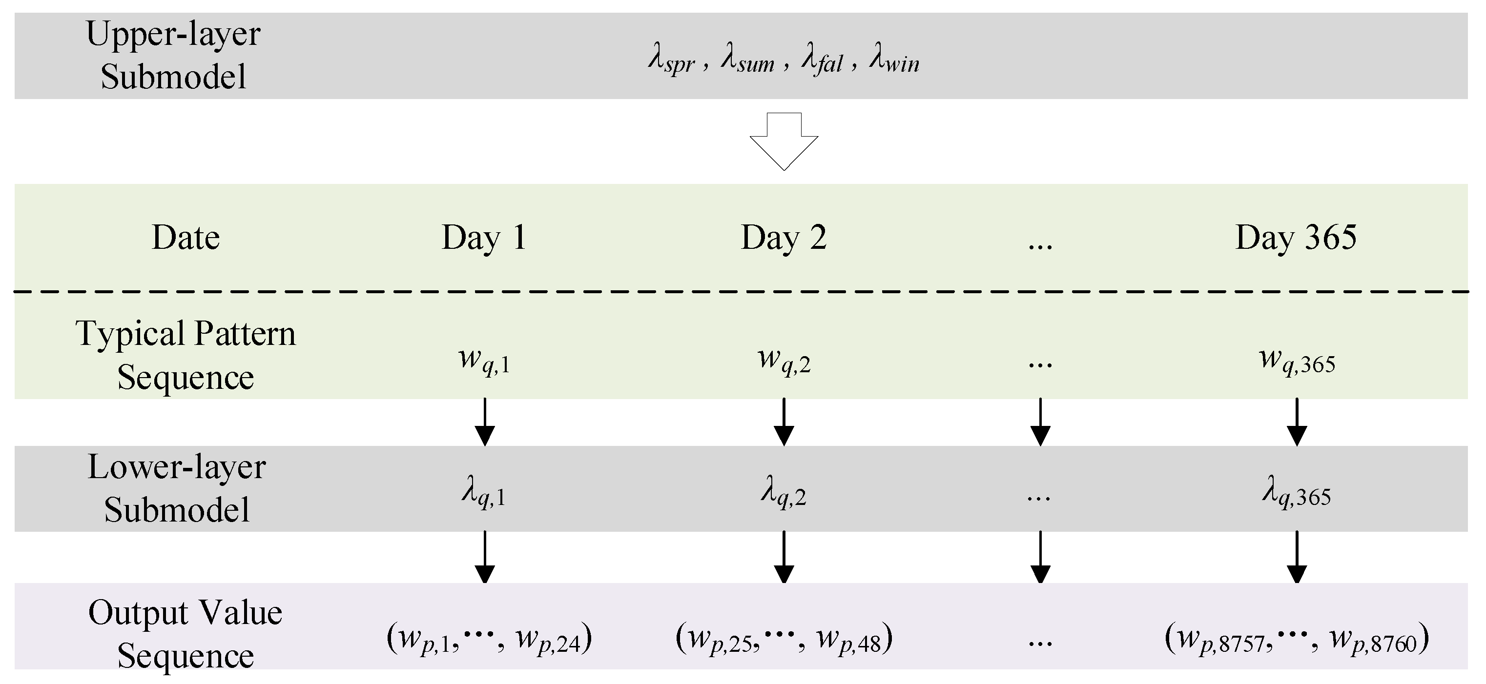The simulation process employs Monte Carlo sampling in two stages: first, generating a typical output pattern sequence Wq for all 365 days using the quarterly discrete HMM, then producing an 8760-h power output sequence Wp for multiple wind farms throughout the year using the GMM–HMM, where the daily power output in conditioned on the previously generated output pattern sequence. The hierarchical structure of the dual-layer model for simulating multi-wind farm power output time series is shown in Figure 1, where $w_{q,1},\dots ,w_{q,365}\in Q$, ${\lambda }_{q,1},\dots ,{\lambda }_{q,365}\in \left\{{\lambda }_1,\dots ,{\lambda }_R\right\}$.

4.1. Scenario Generation for Typical Power Output Pattern Sequences

For a scenario length of Y_spr days in spring, the scenario generation process is as follows:

(1) Calculate the cumulative state transition matrix ${\mathit{C}}_{spr}={\left[c_{spr,ij}\right]}_{N\times (N+1)}$ based on the state transition probability matrix ${\mathit{A}}_{spr}={\left[a_{spr,ij}\right]}_{N\times N}$ of ${\lambda }_{spr}$;

(2) Sample the initial state s_spr,1 for day y = 1 based on the initial state probability ${\mathit{\pi }}_{spr}$ of ${\lambda }_{spr}$;

(3) For current day y with a hidden state s_spr,y = s_i, sample from row i of the observation probability matrix B_spr to obtain the current day’s output pattern q_spr,y;

(4) To determine the hidden state for the next day, generate a random number u from uniform distribution U(0,1). Compare u with the elements in row i of C_spr. If u falls between the element in column j j + 1 of row i, set the hidden state s_spr,y+1 for the next day to s_j;

(5) Repeat steps 3–4 until y equals Y_spr.

These steps are executed sequentially for all four seasons using their respective models. The resulting seasonal scenarios are then concatenated to generate a complete 365-day typical output pattern sequence for the entire year.

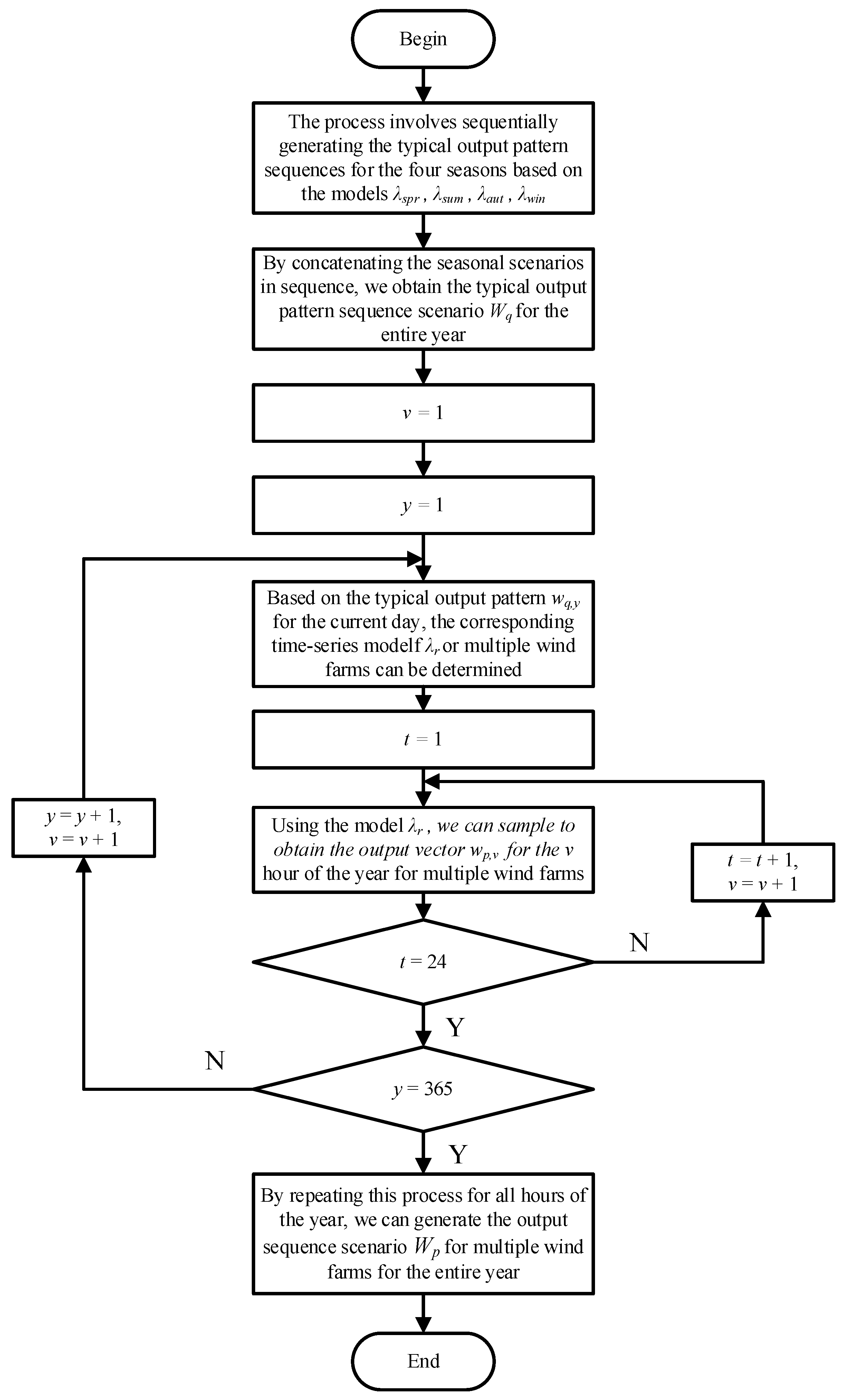
4.2. Generation of Power Output Numerical Sequence Scenarios

The annual wind power output sequence of 8760 h is denoted as $W_p=(w_{p,1},\dots ,w_{p,v},\dots ,w_{p,8760})$, where v represents the hour index. The steps for generating the multi-wind farm output sequence scenario are as follows:

(1) For current day y with typical output pattern w_q,y = q_r, select the corresponding sequence model ${\lambda }_r$ for multi-wind farm power output.

(2) Calculate the cumulative state transition matrix ${\mathit{C}}_r={\left[c_{r,ij}\right]}_{N\times (N+1)}$ from state transition probability matrix ${\mathit{A}}_r={\left[a_{r,ij}\right]}_{N\times N}$ associated with ${\lambda }_r$.

(3) Sample the initial hidden state $s_{p,v}^1$ for current day using initial state probability distribution ${\mathit{\pi }}_r$ of the model.

(4) Sample the Z-dimensional power output vector w_p,v of the multi-wind farms at the v-th hour of the year from the observation probability distribution b_i corresponding to the hidden state $s_{p,v}^1$ at time t.

(5) To determine the hidden state for the next time step, generate a random number x from the uniform distribution U (0,1). Compare x with the elements of the i-th row of C_r. If x falls between the j-th and the (j + 1)-th element of the i-th row, set the hidden state $s_{p,v+1}^{t+1}$ as $s_{p,v}^1$ for the next moment.

(6) Check whether t ≤ 24. If not, then t = t + 1, v = v + 1, and returns to step 4. If t ≤ 24, then y = y + 1, t = 1, v = v + 1, and returns to step 1. Continue the iterative process until y = 365.

The complete process flowchart is illustrated in Figure 2.

4.3. Scenario Evaluation Indicators

4.3.1. Randomness Indicators

The root mean square error (RMSE) and mean absolute error (MAE) are employed to quantitatively access the discrepancy between the generated scenarios and actual scenarios. The RMSE is particularly sensitive to large deviations, making it effective for evaluating instances where the generated power values exhibit substantial departures from the actual measurements. The mathematical formulation of RMSE is presented in Equation (16). The MAE provides a measure of the average difference between the generated scenarios and the actual scenarios. The mathematical expression for MAE is given in Equation (17).

Where w_act,v is the actual power output vector of the multi-wind farms at the v-th hour.

$$RMSE=\sqrt{{\displaystyle \frac{1}{8760}}{\displaystyle \sum _{v=1}^{8760}‖w_{act,v}-w_{p,v}‖}},$$

(16)

$$MAE={\displaystyle \frac{1}{8760}}{\displaystyle \sum _{v=1}^{8760}‖w_{act,v}-w_{p,v}‖},$$

(17)

4.3.2. Statistical Characteristics Indicators

The Wasserstein distance between the probability distribution function of the generated and historical power outputs serves as a metric to evaluate the statistical characteristics of the scenarios. The Wasserstein distance measure effectively quantifies the structural discrepancies between two probability distributions. Through computing the Wasserstein distance between the distribution of generated scenarios and historical data, the fitting degree of the generated scenarios to the historical data distribution characteristics is assessed. This assessment validates the capability of the generated scenarios to preserve the essential statistical characteristics inherent in the historical observations.

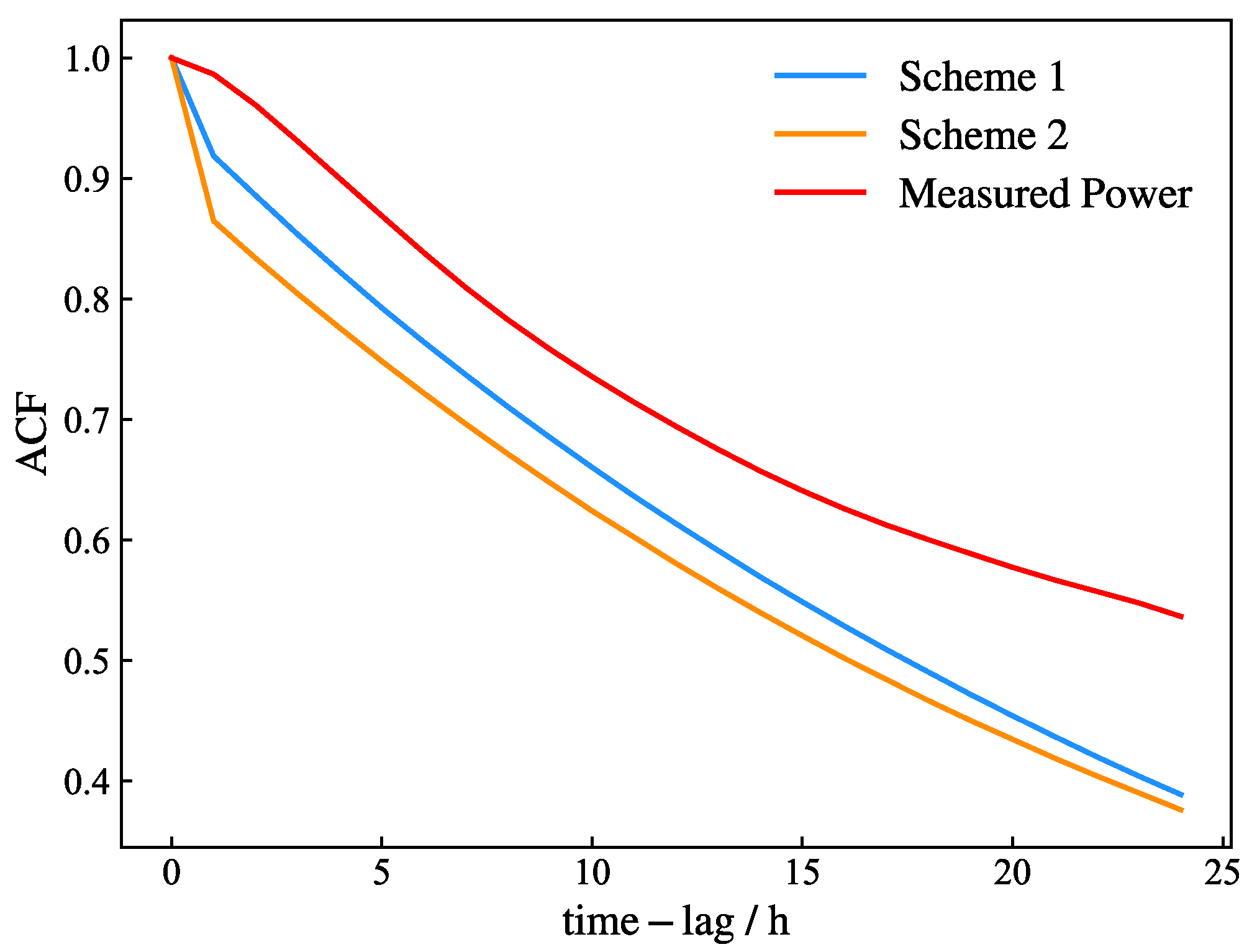
4.3.3. Temporal Characteristics Indicators

The temporal dependency structure of wind power output scenarios can be quantitatively characterized using the autocorrelation function (ACF), which captures the sequential relationships inherent in time series data. For a time series {u₁, …, u_t, …, u_n}, the ACF at lag l is mathematically formulated in Equation (18).

$$\mathrm{ACF}(l)={\displaystyle \frac{\mathrm{cov}\left(u_t,u_{t-l}\right)}{\mathrm{var}\left(u_t\right)}},$$

(18)

where $\mathrm{cov}(•)$ denotes the covariance; $\mathrm{var}(•)$ denotes the variance.

4.3.4. Correlation Indicators

The cross-correlation function (CCF) characterizes the dynamic correlation structure between two time series as a function of their temporal displacement. The CCF is introduced in this paper to quantify the spatiotemporal dependencies between power output sequence scenarios across multiple wind farms. For two time series {u₁, …, u_t, …, u_n} and $\left\{u_1^{\prime },\dots ,u_t^{\prime },\dots ,u_n^{\prime }\right\}$, the CCF at lag l is mathematically expressed in Equation (19)

$$\mathrm{CCF}(l)={\displaystyle \frac{\mathrm{cov}\left(u_t,u_{t-l}^{\prime }\right)}{\sqrt{\mathrm{var}\left(u_t\right)\mathrm{var}\left(u_t^{\prime }\right)}}}.$$

(19)

5. Case Study Analysis

5.1. Case Overview

The case study is based on historical power output data from two wind farms in a province in southern China, covering the period from 2021 to 2023 with a sampling resolution of 1 h. The Z-score method is used to identify and remove outliers from the data. To mitigate the inherent randomness of the Monte Carlo sampling method, the model was trained using historical data from 1 January 2021 to 31 December 2022 and 100 sets of joint wind farm power output sequence scenarios for the entire year of 2023 (each containing 8760 h) were generated. All performance metrics reported later are the averages of these 100 scenarios. The simulation was conducted in a Python 3.10 environment on a computer equipped with an AMD Ryzen™ 5 5600 H CPU, 16.00 GB of RAM, and running Windows 11 Home Chinese Edition. Empirical tests indicate that the model training phase took 42 s, while the scenario generation process took 266 s. Since the number of hidden states in the HMM and the number of Gaussian components in the GMM are key factors affecting the model performance, the discrete HMM state number as well as the state and Gaussian component numbers of the GMM-HMM were selected based on the Bayesian information criterion (BIC).

5.2. Modeling and Analysis of Typical Output Patterns

Based on the method described in Section 2.2, the dimensionality of the historical power output feature matrix was first reduced and the optimal number of clusters was determined through cluster validity analysis. Figure 3 illustrates the decreasing rate of the SSE as the number of clusters increases. It can be observed from the figure that when the number of clusters exceeds 4, the rate of decrease in SSE gradually slows down, indicating that further increasing the number of clusters yields limited improvements in model accuracy. Therefore, the number of clusters was set to 4, partitioning the historical power output sequences into 4 typical daily types.

Based on this approach, the historical daily type sequence was segmented by quarter and modeled using a discrete HMM. Subsequently, a seasonal model was employed to simulate and generate a 365-day daily type sequence for the entire year. Figure 3, Figure 4, Figure 5 and Figure 6 compare the occurrence probabilities of each daily type between the actual data and the generated sequence. It can be observed that the daily type sequence produced by the proposed model closely reproduces the distribution of daily types in the actual data, with the occurrence probabilities of each daily type being essentially consistent with the real data. This indicates that the proposed model can accurately describe the variation patterns of typical daily types in the output of multiple wind farms.

5.3. Comparison of Multi-Wind Farm Long-Term Power Output Sequence Scenario Generation Methods

To evaluate the efficacy and validity of the proposed methodology, the following two comparative simulation schemes are constructed based on the data and parameters specified in Section 4.1:

Scheme 1: using the proposed method that accounts for spatiotemporal correlations and multiscale characteristics for generating long-term power output sequence scenarios of multiple wind farms, annual power output sequence scenarios for multiple wind farms are generated.

Scheme 2: using the method proposed in [5], which considers correlation in the generation of power output time series for multiple wind farms, annual power output sequence scenarios for multiple wind farms are generated.

5.3.1. Randomness Comparison

The statistical indicators quantifying the randomness of scenario sets generated by both schemes are presented in

Table 1. Comparison of randomness indicators.

Scenario Generation Scheme	RMSE	MAE
Scheme 1	0.23	0.17
Scheme 2	0.28	0.21

. The closer the indicator is to 0, the closer the prediction result is to the actual situation, that is, the higher the prediction accuracy is. The scenario set generated using the proposed methodology demonstrates superior performance, achieving a 17.8% reduction in RMSE and a 19.0% reduction in MAE compared to Scheme 2. This enhanced accuracy can be attributed to the methodological approach of segmenting and independently modeling typical power output modes, which effectively mitigates the performance degradation typically caused by intermodal variations. Consequently, the proposed method exhibits superior precision in scenario generation.

5.3.2. Statistical Characteristics Comparison

Table 2. Comparison of Wasserstein distance.

Scenario Generation Scheme	Wasserstein Distance
Scheme 1	0.043
Scheme 2	0.054

shows the Wasserstein distance between the empirical distribution of the scenario sets generated by the two schemes and the historical power output empirical distribution. The smaller the Wasserstein distance, the higher the fitting degree to the statistical characteristics of the historical data. The Wasserstein distance between the empirical distribution of the scenario set generated by the proposed method in this paper and the historical power output empirical distribution is 0.043, representing a 20% reduction compared to Scheme 2. This significant improvement demonstrates the superior capability of the proposed method in capturing the intrinsic statistical properties of wind power generation patterns.

Table 3. Comparison of seasonal average power output.

Scenario	Spring	Summer	Fall	Winter
Historical Power Output Sequence	0.2	0.14	0.22	0.29
Scenario Set of Scheme 1	0.19	0.11	0.22	0.29
Scenario Set of Scheme 2	0.2	0.19	0.19	0.19

presents the seasonal average power output comparison between the historical data and scenarios generated by the two schemes for Wind Farm 1. The proposed method successfully captures the distinct seasonal patterns observed in the historical data, particularly the lower generation levels during spring and summer months and higher output during fall and winter periods. In contrast, Scheme 2 fails to accurately reproduce these characteristic seasonal variations in wind power generation. This demonstrates the proposed method’s superior capability in preserving temporal patterns across different temporal scales.

5.3.3. Temporal Characteristics Comparison

Figure 5 illustrates the autocorrelation function (ACF) of the historical power output sequence and generated scenario sets for Wind Farm 2, computed across lag times ranging from 0 to 24 h. Both schemes successfully reproduce the characteristic strong temporal dependency of wind power generation, as evidenced in ACF by the gradual decay in autocorrelation with increasing lag time. However, the scenario set generated by the proposed method exhibits consistently higher ACF values across most lag times compared to Scheme 2, demonstrating its superior capability in preserving the temporal dependencies inherent in wind power generation patterns.

Figure 5. ACF of Wind Farm 2.

Figure 5. ACF of Wind Farm 2.

5.3.4. Correlation Comparison

Figure 6 depicts the CCF between the generated scenario sets and historical power output sequence across lag times from 1 to 24 h. The scenario set generated by the proposed method consistently demonstrates higher CCF values compared to Scheme 2 across the majority of lag times, validating the superior performance of the proposed method in capturing the temporal correlation structure of wind power generation.

Figure 6. CCF of power output sequences of Wind Farm 1 and Wind Farm 2.

Figure 6. CCF of power output sequences of Wind Farm 1 and Wind Farm 2.

6. Discussion

This paper proposes a method for generating medium- and long-term output sequence scenarios of multiple wind farms based on a two-stage HMM. To account for the seasonal and daily scale characteristics of wind power output, feature extraction and clustering methods are used to extract typical patterns of daily wind power output. A discrete HMM is employed to model the transition of typical daily output patterns within each quarter. To account for the spatiotemporal correlation of the output of multiple wind farms, a GMM–HMM is used to model the numerical fluctuations of the output of multiple wind farms at each time step. Based on the two-stage time-series model, medium- and long-term output sequence scenarios of multiple wind farms are obtained through quarterly and daily sampling. Compared to the model proposed in Reference [5], the two-layer time-series model proposed in this paper can better describe the multi-time-scale characteristics of wind power output. Practical examples demonstrate that the method proposed in this paper outperforms the comparison method in terms of statistical characteristics, temporal characteristics, sequence correlation, and seasonal characteristics. However, in the model of this paper, whether it is the discrete HMM or the GMM–HMM, the hidden states are represented by discrete values ranging from 1–N, which lacks a detailed characterization of the state transition mechanism and does not perform analytical modeling of the key factors affecting wind power output. Future research can further explore more refined methods for modeling hidden states to enhance the model’s ability to describe the variation patterns of wind power output.

7. Conclusions

This paper presents a novel scenario generation method for long-term multi-wind farm power output sequences that integrates daily power output patterns with intraday fluctuations. The case studies yield the following conclusions:

(1) The proposed mode-specific modeling approach enhances accuracy by addressing each typical pattern independently, thereby avoiding the sample interference that commonly occurs in aggregate modeling. This targeted approach significantly improves the model’s ability to capture distinct operational characteristics.

(2) The method proposed in this paper adopts a two-layer modeling framework. While considering the spatiotemporal correlation of the power outputs of multiple wind farms, it also takes into account both the short-term stochastic characteristics and long-term changing trends of wind power generation, thus enabling a more accurate description of wind power characteristics.

(3) Comparative analysis across multiple performance metrics demonstrates that, compared to the comparison methods, the proposed method reduces the error index by 18% and decreases the Wasserstein distance between the empirical distribution of the scenario set and the historical output distribution by 20%, effectively improving the quality of the scenarios. The case studies show that the proposed method can accurately restore the statistical characteristics, temporal characteristics, sequence correlation, and seasonal characteristics of the output of multiple wind farms. These high-quality scenarios provide valuable insights for power system operation simulation, enabling more robust generation scheduling strategies and enhanced wind power integration capabilities.