Efficient Short-Term Wind Power Prediction Using a Novel Hybrid Machine Learning Model: LOFVT-OVMD-INGO-LSSVR

Abstract

Accurate wind power forecasting (WPF) is crucial to enhance availability and reap the benefits of integration into power grids. The time lag of wind power generation lags the time of wind speed changes, especially in ultra-short-term forecasting. The prediction model is sensitive to outliers and sudden changes in input historical meteorological data, which may significantly affect the robustness of the WPF model. To address this issue, this paper proposes a novel hybrid machine learning model for highly accurate forecasting of wind power generation in ultra-short-term forecasting. The raw wind power data were filtered and classified with the local outlier factor (LOF) and the voting tree (VT) model to obtain a subset of inputs with the best relevance. The time-varying properties of the fluctuating sub-signals of the wind power sequences were analyzed with the optimized variational mode decomposition (OVMD) algorithm. The Northern Goshawk optimization (NGO) algorithm was improved by incorporating a logical chaotic initialization strategy and chaotic adaptive inertia weights. The improved NGO algorithm was used to optimize the least squares support vector regression (LSSVR) prediction model to improve the computational speed and prediction results. The proposed model was compared with traditional machine learning models, deep learning models, and other hybrid models. The experimental results show that the proposed model has an average R² of 0.9998. The average MSE, average MAE, and average MAPE are as low as 0.0244, 0.1073, and 0.3587, which displayed the best results in ultra-short-term WPF.

1. Introduction

Wind power provides a promising solution for the global energy crisis and environmental pollution which is known as one of the cleanest and safest sustainable energy [1,2]. However, the unpredictable nature of meteorological factors results in random fluctuations in wind power generation, which can significantly hinder the integration of wind power into the grid and impede the stable operation of power systems [3,4]. Therefore, accurate forecasting of wind power is crucial for energy consumption reduction, power system operations optimization, and sustainable development promotion [5,6,7].

Wind power forecasting (WPF) can be approached as a multiple regression problem that requires vast amounts of historical wind power data [8]. Prediction methods based on traditional physical modeling are computationally complex with weak generalization capabilities [9,10]. However, data-driven machine learning models offer new possibilities for accurately predicting wind power [11,12]. Heinermann et al. [13] utilized a combination of K-nearest neighbor (KNN), decision tree (DT), and support vector regression (SVR) algorithms. The least absolute shrinkage selection operator (LASSO), KNN, extreme gradient boosting (XGBoost), random forest (RF), and SVR algorithms for WPF were used [14]. Lu et al. [15] combined spatio-temporal analysis, multicategory support vector machine (MSVM), and grey wolf optimization (GWO) to forecast output wind power from multiple wind farms. Wen et al. [16] employed k-means-hierarchical clustering (KHC), singular value decomposition (SVD), and SVR models to extract the dominant part of the generating units and predicted output power. Chen et al. [17] proposed a hybrid WPF model based on a multi-resolution multi-learner ensemble (MRMLE) and adaptive model selection (AMS) for power forecasting.

Machine learning models have made significant strides in wind power forecasting. However, there is still ample potential to enhance the predictive accuracy of the algorithms amid the intricacies of meteorological data and the high-dimensional nature of wind power datasets. Recent deep learning models can automatically extract data features to improve the forecasting accuracy of wind power generation [18]. Yu et al. [19] utilized wavelet transform (WT) for decomposing original wind speed historical data and integrated it with the Elman neural network (ENN) to predict wind power. Wang et al. [20] applied an enhanced version of the sparrow search algorithm (SSA) to improve the performance of a long short-term memory (LSTM) network. The gate recurrent unit (GRU) has fewer parameters and can be faster to train compared to LSTM. Xiao et al. [21] combined feature-weighted principal component analysis (WPCA) with a modified GRU neural network model and used the particle swarm optimization (PSO) algorithm to optimize the hyperparameters of this model. In general, deep learning algorithms tend to have higher accuracy in predicting wind power as compared to traditional machine learning algorithms.

The deep learning algorithms have the problems of high complexity and training costs, which means it is difficult to develop and implement effective models, especially as available computing resources are scarce. The diverse time-frequency signal decomposition methods have been integrated into the models to improve the accuracy of WPF and the reliability of data processing in different dimensions. Wang et al. [22] utilized the multi-objective bat algorithm (MOBA) to optimize an artificial neural network by combining it with singular spectrum analysis (SSA) to enhance the accuracy and stability of their model. Naik et al. [23] combined empirical mode decomposition (EMD) with kernel ridge regression (KRR) to predict short-term wind speed and wind power. The combined phase space reconstruction (PSR), variational mode decomposition (VMD), and genetic algorithm optimized wavelet neural networks (GAWNN) to improve overall prediction accuracy [24]. The time-frequency signal decomposition technique has been proven to reduce data instability and improve the robustness of the WPF model. Wind farms operate within spot electricity markets and longer-term wind power forecasts cannot meet the instantaneous supply and demand balance in the power system. Ultra-short-term WPF has gained the attention of researchers due to its improved alignment with actual wind farm demand. Wei et al. utilized the combination of maximum information coefficients (MIC) with multi-task learning (MTL) and LSTM networks to enhance the accuracy of ultra-short-term WTF [25]. Lu et al. [26] used complete ensemble empirical mode decomposition with adaptive noise (CEEMDAN) and improved cuckoo search (ICS) strategies to optimize the least squares support vector machine (LSSVM) to achieve better prediction results. Niu et al. incorporated an improved VMD algorithm into a bidirectional long short-term memory (BiLSTM) to enhance the accuracy of WPF [27]. The bidirectional gated recurrent unit (BiGRU) had an advantage in terms of training speed and number of parameters compared to BiLSTM. Yu et al. [28] proposed a new model for the optimization of attention mechanisms based on BiGRU and RF-WOA-VMD. Liu et al. [29] eliminated high wind speed and low power as well as low wind speed and high power data, which combined encoder–decoder (ED), BiGRU, and feature–temporal attention (FT-Attention) to predict wind power with good prediction results.

Although machine learning, deep learning, and time-frequency signal decomposition techniques have achieved significant progress in ultra-short-term WPF, there still exist some limitations. Wind power generation has time lags and inertia effects, which must be considered during analysis. Outliers should not be directly removed, which should be evaluated based on the specific situation. Ultra-short-term wind power forecasts are highly sensitive to sudden changes and outliers in historical meteorological data. Existing models often overlook the importance of targeted data pre-processing, which can have a significant impact on the reliability and accuracy reliability of the forecasting model. Ultra-short-term WPF is influenced by multiple complex factors. A single forecasting model may not be enough to fully capture the multi-dimensional data features required for accurate prediction. The non-linear relationship among the meteorological factors, seasonal weather and wind power generation remains unknown.

To tackle the limitations, this study proposes a novel hybrid machine learning model LOFVT-INGO-OVMD-LSSVR, which aims to improve ultra-short-term WPF accuracy while reducing model complexity and minimizing training costs. The raw wind power data were first filtered and classified by a data pre-processing model. Then the optimized VMD module was used to decompose the pre-processed wind power data into multiple sub-series for analysis. Finally, the improved LSSVR model was utilized to fit the non-linear relationship between meteorological data and wind power to enable more accurate predictions of wind power. The innovation of this article is as follows:

(1)

The LOF algorithm was employed to filter the wind power data features to preserve reasonable data for sudden changes in wind speed while eliminating outliers.

(2)

The VT algorithm was utilized to categorize wind power data according to seasonal types and weather conditions to develop a corresponding wind electricity forecasting model.

(3)

The optimized VMD algorithm was used to perform multimodal decomposition of the historical wind power data, which can enable analysis of the time-varying characteristics of wind power time series under different sub-signals to enhance the predictive performance of the model.

(4)

The NGO algorithm was enhanced by incorporating logical chaos initialization and chaotic adaptive inertia weights. The improved algorithm was employed to optimize the LSSVR model. The goal is to accelerate the convergence of the model training process and prevent the model from being trapped in a local optimum solution.

2. Methodology

2.1. Data Pre-Processing

2.1.1. Local Outlier Factor (LOF)

The LOF algorithm is an unsupervised technique employed for detecting outliers. It operates by computing the local density deviation of a data point in relation to its surrounding area [30]. Specifically, for a fixed k value, the k-distance domain of a given object (o) can be denoted as follows:

$$N_{k-distance\left(o\right)}\left(o\right)=\left\{p\in D\backslash \left\{o\right\}|d\left(o,p\right)<k-distance\left(o\right)\right\}$$

(1)

where object $p$ represents the k-nearest neighbor of object $o$.

The reachability distance of object $p$ from object $o$ can be expressed as follows:

$$reach-{dist}_k\left(p,o\right)=\max \left\{k-distance\left(o\right),d\left(p,o\right)\right\}$$

(2)

The locally reachable density of object $o$ is formulated as:

$${lrd}_{MinPts}\left(o\right)={\displaystyle \frac{1}{\frac{{\sum }_{p\in N_{MinPts}\left(o\right)}reach-{dist}_{MinPts}\left(p,o\right)}{\left|N_{MinPts}\left(o\right)\right|}}}$$

(3)

where $N_{MinPts}\left(o\right)$ denotes the nearest k-domain points of object $o$.

The local outlier factor of object $o$ is expressed as:

$${LOF}_{MinPts}\left(o\right)={\displaystyle \frac{{\sum }_{p\in N_{MinPts}\left(o\right)}\frac{{lrd}_{MinPts}\left(p\right)}{{lrd}_{MinPts}\left(o\right)}}{\left|N_{MinPts}\left(o\right)\right|}}$$

(4)

The local anomaly factor of object $o$ denotes the level of anomaly of data point $o$. A value of ${LOF}_{MinPts}\left(o\right)$ is close to 1 indicates that object $o$ is akin to the domain density, whereas a value of ${LOF}_{MinPts}\left(o\right)$ greater than 1 suggests that data point $o$ is more likely to be an outlier.

2.1.2. Savitzky–Golay Filter

The Savitzky–Golay filter is a filtering technique that can be used to smooth data while preserving the underlying trend and signal width [31]. By fitting a low-order polynomial to a contiguous subset of adjacent data points with linear least squares, it can effectively improve the accuracy of the data without altering its essential features. Notably, the Savitzky–Golay filter has been found to be particularly effective in addressing timing series issues. The specific formula for the Savitzky–Golay filter is as follows.

$$X_{k,smooth}={\displaystyle \frac{1}{H}}\sum _{i=-m}^{+m}{X}_{k+i}\ast h_i$$

(5)

where $X_{k+i}$ represents a continuous subset of adjacent data points, ${\displaystyle \frac{h_i}{H}}$ represents the smoothing factor, $h_i$ represents the unit impulse response, “$\ast$” represents the convolution operator.

2.1.3. Voting Tree Algorithm (VT)

VT is a combination strategy used in integrated learning for classification problems [32]. This approach leverages the principle of majority rule and minimizes variance by integrating multiple models resulting in improved model robustness. VT has demonstrated impressive performance in various classification scenarios. The VT model comprised logistic regression [33], RF [34] and SVC [35] models in this study.

Logistic regression is a classification method that assumes the data follows the Bernoulli distribution and is based on the derivation of maximum likelihood estimates. The model parameters are obtained by applying gradient descent through the logarithmic variation of the likelihood function to classify the data. Random forest is a classification algorithm that employs multiple decision trees to train and predict samples, which determines the relevance of each data feature and assigns weights to different features to obtain classification results. SVC is a widely used classifier that segments data samples by finding a hyperplane with the principle of maximizing the margin. This study integrated the three algorithms mentioned above to classify wind power data features and obtained the most relevant subset of data.

2.1.4. L2 Normalization

L2 normalization is commonly employed in data preprocessing and feature normalization. The formula for L2 normalization is as follows:

$$norm\left(X_i\right)=\sqrt{x_1^2+x_2^2+\dots +x_n^2}$$

(6)

where $X_i$ represents the data in different dimensions, $i$ represents the dimension of the data, $n$ represents the number of data under each dimension.

$$\begin{gathered} norm\left(X_i^{\prime }\right)={\displaystyle \frac{\sqrt{x_1^2+x_2^2+\dots +x_n^2}}{norm\left(X_i\right)}} \\ =\sqrt{x_1^{\prime 2}+x_2^{\prime 2}+\dots +x_n^{\prime 2}} \end{gathered}$$

(7)

The L2 parametric product of the wind power data ($norm\left(X_i\right)$) and the model prediction result can be utilized to achieve inverse normalization in order to obtain the original data. Moreover, as it is independent of their size, $norm\left(X_i\right)$ can also be utilized as a scale factor to achieve the desired output as cosine similarity can measure the degree of similarity between two non-zero vectors.

2.2. Improved Northern Goshawk Optimization Algorithm (INGO)

The NGO algorithm can be effectively applied to solve spatial function optimization problems and objective optimization problems [36]. To prevent the NGO from converging to local optima, logical chaotic initialization and chaotic adaptive inertia weights were used.

Exploration phase: This phase is crucial for enhancing the exploration capability of the algorithm. In order to achieve this, the selection in the search space is conducted at random with the following equation.

$$P_i=X_k,i=\mathrm{1,2}\dots ,N k=\mathrm{1,2}\dots ,N$$

(8)

$$x_{i,j}^{new,P1}=\left\{\begin{array}{c}{x}_{i,j}+r\left(p_{i,j}-I{x}_{i,j}\right),F_{P_i}<F_i\\ x_{i,j}+r\left(x_{i,j}-p_{i,j}\right),F_{P_i}\ge F_i\end{array}\right.$$

(9)

$$X_i=\left\{\begin{array}{c}{X}_i^{new,P1},F_i^{new,p1}<F_i\\ X_i, { F}_i^{new,p1}\ge F_i\end{array}\right.$$

(10)

where $P_i$ denotes the position of the $i$th prey, $F_{P_i}$ denotes the objective function value of the $i$th prey, $X_i^{new,P1}$ denotes the new position of the $i$th northern goshawk, $x_{i,j}^{new,P1}$ denotes the new position of the $i$th northern goshawk at the $j$th latitude, $F_i^{new,p1}$ denotes the updated objective function value of the $i$th northern hawk, $r$ is a random number in the range [0,1], $I$ is a random integer of 1 or 2.

Development phase: This phase aims to enhance the algorithm’s proficiency in locally searching the search space. The formula for this phase is as follows.

$$x_{i,j}^{new,P2}=x_{i,j}+R\left(2r-1\right)x_{i,j}$$

(11)

$$X_i=\left\{\begin{array}{c}{X}_i^{new,P2},F_i^{new,p2}<F_i\\ X_i, { F}_i^{new,p2}\ge F_i\end{array}\right.$$

(12)

where $X_i^{new,P2}$ represents the new position of the $i$th northern goshawk, $x_{i,j}^{new,P2}$ represents the new position of the $i$th northern goshawk at the $j$th latitude, $F_i^{new,p2}$ represents the objective function value of the updated $i$th northern hawk, $R$ is the weighting factor.

2.2.1. Logical Chaos Initialization

The properties of chaos of randomness, non-periodicity and non-convergence are often utilized in nonlinear systems to enhance the performance of algorithms [37]. This study employed logistic chaotic mapping to generate a more uniformly distributed population, which facilitated a faster convergence rate for the algorithm. The formula is as follows:

$$x_{i+1}=4x_i\left(1-x_i\right)$$

(13)

The use of logistic chaotic mapping replaces the randomly generated population during initialization in the NGO algorithm. This enhances the diversity of the initial population and reduces the likelihood of the algorithm converging to local optimum solutions. Consequently, the optimization performance of the NGO algorithm is improved.

2.2.2. Chaotic Adaptive Inertia Weights

To optimize the weight coefficients of the NGO, the chaotic adaptive inertia weighting method was utilized, which can be expressed as follows:

$$R={\omega }_{min}{\left({\displaystyle \frac{{\omega }_{max}}{{\omega }_{min}}}\right)}^{\left(1-{\displaystyle \frac{t}{T}}+\left({\displaystyle \frac{X_{best}-X_i}{X_{best}}}\right)\right)}$$

(14)

where ${\omega }_{min}$ represents the minimum weight coefficient, ${\omega }_{max}$ represents the maximum weight coefficient, $t$ stands for the current training iteration, T denotes the total number of training iterations, $X_{best}$ indicates the current global optimal position, and $X_i$ denotes the current position being evaluated.

During the initial iterations, the value of $R$ is primarily determined by the maximum weight coefficient ${\omega }_{max}$. This strategy helps prevent the algorithm from getting trapped in local minima during the early stages of the search. As the iterations progress, R gradually decreases while the weight coefficients are adjusted based on the current search situation by calculating the ratio ${\displaystyle \frac{X_{best}-X_i}{X_{best}}}$. The complete INGO algorithm is presented in Algorithm 1.

Algorithm 1. INGO Algorithm Process

Start INGO. 1. Input the parameters of the optimization problem. 2. Input the INGO population size (N) and the number of iterations (T). 3. Initialize the position of the northern eagle using the logistic chaos Equation (13). 4. For t = 1: T 5.        Generate the position of the prey at random. 6.        Phase 1: Identifying prey(exploration phase). 7.        For j = 1: N 8.             Calculate new status of the $j$th dimension using Equation (9). 9.        End. 10.       Update the $i$th population member using Equation (10). 11.       Phase 2: Tracking prey(development phase). 12.       For j = 1: N 13.             Update the chaotic adaptive inertia weights using Equation (14). 14.             Calculate new status of the $j$th dimension using Equation (11). 15.       End. 16.       Update the $i$th population member using Equation (12). 17.       Update best candidate solution. 18. End. 19. Output best candidate solution obtained by INGO. End INGO.

2.3. Variational Mode Decomposition (VMD)

VMD is a fully non-recursive variational modal decomposition algorithm that can decompose and extract multiple modes [38]. The intrinsic modal function for a finite bandwidth in VMD is defined.

$$u_k\left(t\right)=A_k\left(t\right)\cos \left({\varphi }_k\left(t\right)\right)$$

(15)

where $A_k\left(t\right)$ represents the amplitude of $u_k\left(t\right)$ and ${\varphi }_k\left(t\right)$ represents the phase of $u_k\left(t\right)$. The process of implementing the modal decomposition is as follows:

$$\left\{\begin{array}{c}\begin{array}{c}min\\ \left\{u_k\right\},\left\{{\omega }_k\right\}\end{array}\{{\displaystyle \sum _k}\parallel {{\partial }_t\left[\left(\delta \left(t\right)+{\displaystyle \frac{j}{\pi t}}\right)\ast u_k\right]e^{-j{\omega }_{k}t}\parallel }^2\}\\ S.T. {\displaystyle \sum _k}{u}_k=x(t)\end{array}\right.$$

(16)

where $u_k$ represents the decomposed signal, ${\omega }_k$ denotes the center frequency of $u_k$, $\delta \left(t\right)$ stands for the impulse signal, $x\left(t\right)$ is the original undecomposed signal, $e^{-j{\omega }_{k}t}$ denotes the Hilbert transform, $\partial$ denotes the gradient operator, $\ast$ represents the convolution operator.

To discover the optimal solution of the constrained variational problem, Lagrange multipliers and second-order penalty factors are utilized to convert the constrained variational problem into an unconstrained variational problem. The expression for the extended Lagrange is expressed.

$$\begin{gathered} L\left(\left\{u_k\right\},\left\{{\omega }_k\right\},\tau \right)=\alpha \sum _k\parallel {{\partial }_t\left[\left(\delta \left(t\right)+{\displaystyle \frac{j}{\pi t}}\right)\ast u_k\right]e^{-j{\omega }_{k}t}\parallel }^2 \\ +\parallel {s\left(t\right)-\sum _k{u}_k\left(t\right)\parallel }^2+〈\tau \left(t\right),s\left(t\right)-\sum _k{u}_k\left(t\right)〉 \end{gathered}$$

(17)

where $\alpha$ represents a second-order penalty factor, which ensures the accuracy of signal reconstruction, while $\tau \left(t\right)$ represents a Lagrange multiplier that maintains the strictness of the constraints. The frequency domain space yields all the components of the optimal solution as per the following equation.

$${\widehat{u}}_k^{n+1}\left(\omega \right)={\displaystyle \frac{\widehat{s}\left(\omega \right)-{\sum }_{i\ne k}\widehat{u_i}\left(\omega \right)+\frac{\widehat{\tau }\left(\omega \right)}{2}}{1+2\alpha {\left(\omega -{\omega }_k\right)}^2}}$$

(18)

In this equation, ω refers to frequency, while ${\widehat{u}}_k^{n+1}\left(\omega \right)$, $\widehat{s}\left(\omega \right)$ and $\widehat{\tau }\left(\omega \right)$ represent the Fourier transforms of $u_k^n\left(\omega \right)$, $s\left(t\right)$ and $\tau \left(t\right)$, respectively. The central frequency is re-estimated as per each component. ${\omega }_k$ and $\widehat{\tau }$ are updated according to the following equations:

$${\omega }_k^{n+1}={\displaystyle \frac{{\int }_0^{\infty }\omega |{\widehat{u}}_k^{n+1}\left(\omega \right){|}^{2}d\omega }{{\int }_0^{\infty }|{\widehat{u}}_k^{n+1}\left(\omega \right){|}^{2}d\omega }}$$

(19)

$${\widehat{\tau }}^{n+1}={\widehat{\tau }}^n\left(\omega \right)+\tau \left(\widehat{s}\left(\omega \right)-\sum _k{\widehat{u}}_k^{n+1}\left(\omega \right)\right)$$

(20)

The updating process halts when the subsequent equation is satisfied:

$${\displaystyle \frac{{\sum }_k\parallel {{\widehat{u}}_k^{n+1}-{\widehat{u}}_k^n\parallel }_2^2}{\parallel {{\widehat{u}}_k^n\parallel }_2^2}}<\epsilon$$

(21)

where ε denotes the stopping threshold. To sum up, the decomposition layers $k$ and penalty factor $\alpha$ of the signal play a crucial role in determining the effect of modal decomposition.

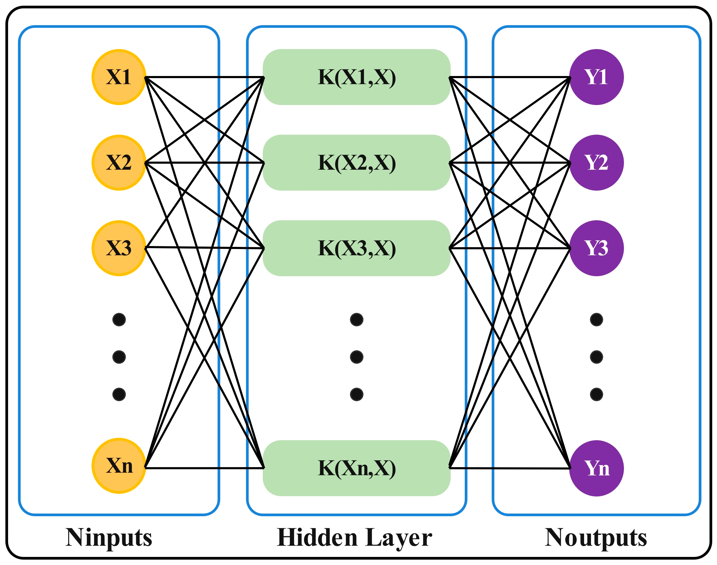
2.4. Least Squares Support Vector Regression Model (LSSVR)

LSSVR is a machine learning technique that utilizes kernel-based ridge regression. Compared to SVM, it converts the inequality constraint into an equation constraint, which greatly simplifies the solution of the Lagrange multipliers [39]. The structure of LSSVR is depicted in Figure 1.

The input variable for LSSVR is the meteorological parameter (X) and the output parameter is wind power generation (Y). The input expression for LSSVR is as follows:

$$f\left(X\right)=\sum _{i=1}^N{\alpha }_{i}K\left(X,X_i\right)+b$$

(22)

where $X$ represents the test input, $X_i\in {data}^n$ represents the meteorological parameter of the input, $K$ represents the kernel function, and $b$ represents the bias. The output expression of LSSVR is as follows:

$$f\left(X\right)=\sum _{i=1}^N{\alpha }_i\exp \left({\displaystyle \frac{-\parallel X-X_i{\parallel }^2}{2{\sigma }^2}}\right)+b$$

(23)

where ${\alpha }_i$ represents the support vector, $\parallel X-X_i{\parallel }^2$ represents the Euclidean parametrization, and $\sigma$ represents the radial basis kernel function width. Through the use of Lagrange duality and Kuhn–Tucker conditions (KKT), the optimization problem can be transformed into the following equation.

$$\begin{array}{c}\mathrm{m}\mathrm{i}\mathrm{n}\\ \omega ,b,{\xi }_i^2\end{array} L_1\left(\omega ,b,\xi \right)={\displaystyle \frac{1}{2}}{\omega }^T\omega +\gamma {\displaystyle \frac{1}{2}}\sum _{i=1}^N{\xi }_i^2$$

(24)

$$S.T y_i={\omega }^T\psi \left(X_i\right)+b+{\xi }_i i=\mathrm{1,2}\dots ,N$$

(25)

where $\omega$ represents the weight vector in the original space, $\gamma$ represents the penalty factor, $\psi \left(X_i\right)$ represents used to map the input to a high-dimensional feature space, and ${\xi }_i$ represents the error variable. The above optimization problem is treated with the Lagrange multiplier method.

$$L\left(\omega ,b,\xi ,\alpha \right)=L_1\left(\omega ,b,\xi \right)-\sum _{i=1}^N{\alpha }_i\left({\omega }^T\psi \left(x_i\right)+b+{\xi }_i-y_i\right)$$

(26)

Based on the KKT condition, the following conclusions are drawn.

$$\left\{\begin{array}{c}\begin{array}{c}{\displaystyle \frac{\partial L}{\partial \omega }}=0\to \omega ={\displaystyle \sum _{i=1}^N}{\alpha }_i\psi \left(x_i\right)\\ {\displaystyle \frac{\partial L}{\partial b}}=0\to {\displaystyle \sum _{i=1}^N}{\alpha }_i=0\end{array}\\ \begin{array}{c}{\displaystyle \frac{\partial L}{\partial {\xi }_i}}=0\to {\alpha }_i=\gamma {\xi }_i i=\mathrm{1,2}\dots ,N\\ {\displaystyle \frac{\partial L}{\partial {\alpha }_i}}=0\to \left({\omega }^T\psi \left(x_i\right)+b\right)+{\xi }_i-y_i=0\end{array}\end{array}\right.$$

(27)

The final result is obtained after eliminating ω and Equation (28).

$$\left[\begin{array}{cc}0& E_M^T\\ E_M& \Omega +{\displaystyle \frac{E_M}{\gamma }}\end{array}\right]\left[{\displaystyle \frac{b}{\alpha }}\right]=\left[{\displaystyle \frac{0}{y}}\right]$$

(28)

where $y=[y_1, y_2\dots , y_N]$, $\alpha =[{\alpha }_1, {\alpha }_2\dots ,{\alpha }_N]$, ${\Omega }_{ij}={\psi \left(x_i\right)}^T\psi \left(x_j\right)$, $E_M={[\mathrm{1,1}\dots ,1]}^T$.

In summary, the penalty factor ($c$) and the width of the kernel function ($g$) play a crucial role in obtaining accurate regression results with the LSSVR model. Here, $c$ represents the tolerance to error, while $g$ denotes the mapping dimension of the low-dimensional sample to the high-dimensional mapping (Wu and Ye, 2016; Ghaedi et al., 2016) [40,41]. Although larger values of $c$ and $g$ may lead to better model training results, there is also an increased risk of overfitting [42]. Therefore, it is vital to carefully choose the appropriate values of $c$ and $g$ during model training.

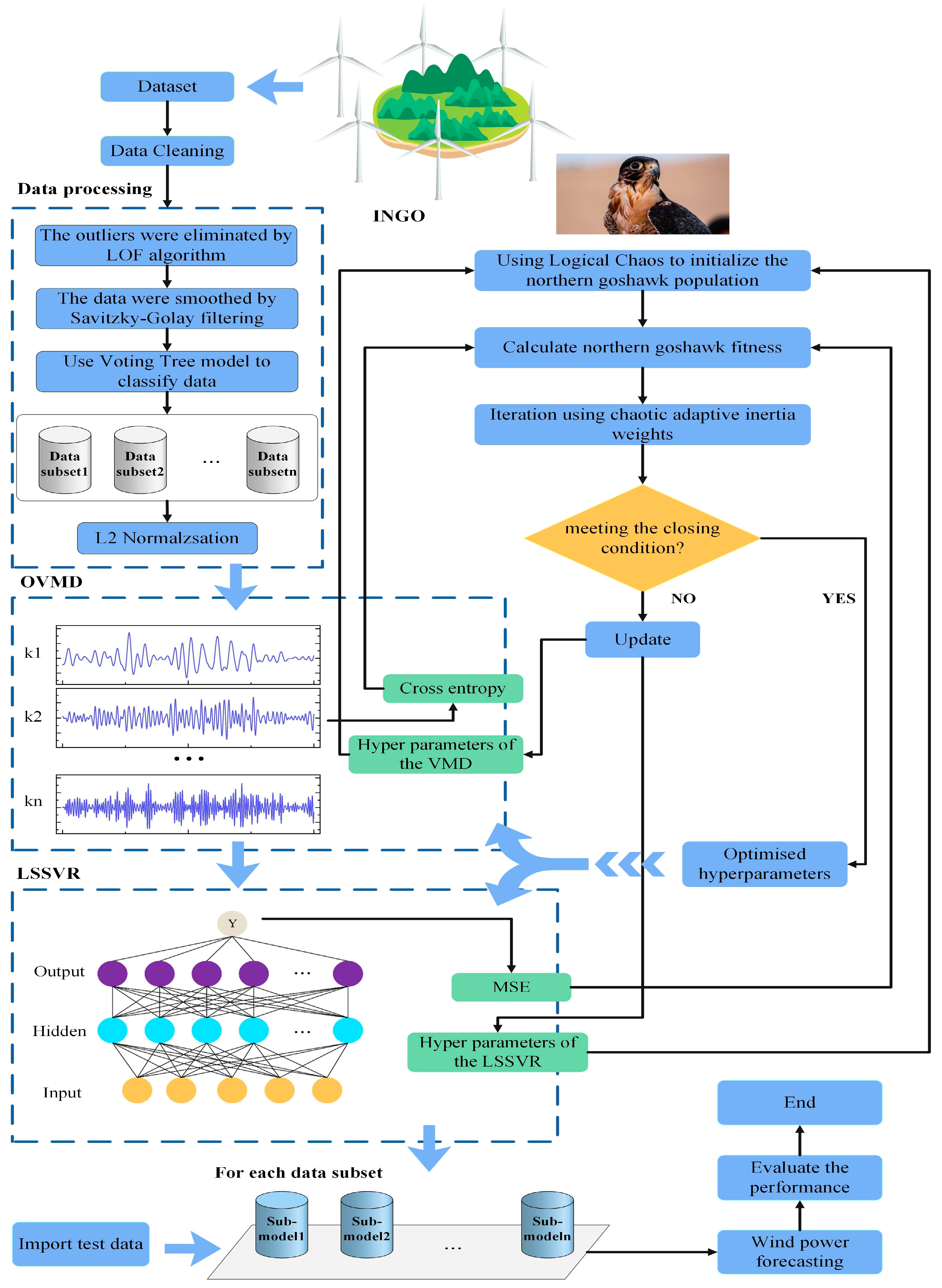
3. Composition of the Proposed Model

To address the issues of extracting relevant feature information from complex data and optimizing the LSSVR model, this study presents a novel hybrid machine learning model LOFVT-INGO-OVMD-LSSVR for ultra-short-term WPF. Figure 2 illustrates the workflow and steps of the proposed model. The model consists of a data processing module, INGO module, OVMD module and LSSVR module. The preprocessing module enhances data quality by eliminating outliers with the LOF algorithm, reducing noise with the Savitzky–Golay filter, classifying data based on weather and seasonal patterns via the VT model to ensure the consistency through L2 normalization. The OVMD module extracts deeper frequency domain features by decomposing the normalized data with the optimal decomposition layers and penalty factor determined with the INGO algorithm. Finally, the LSSVR module leverages INGO to optimize the penalty factor and kernel function bandwidth to improve the overall prediction accuracy.

The roles and inputs/outputs of each component of the process are listed in

Table 1. Roles, inputs, and outputs of each component in the process.

Process	Input	Algorithm	Function	Output
1	Raw data	LOF	Remove outliers and retain reasonable wind power data	Normal data
2	Normal data	SG filter	Eliminate noise interference from the data	Denoised data
3	Denoised data	VT	Divide the data into multiple sub-datasets to reduce model computation	Classified data
4	Classified data	L2 normalization	Normalize multi-dimensional features to the same scale, aiding model learning	Normalized data
5 (for each sub-dataset)	Normalized data	INGO-OVMD	Optimize VMD hyper-parameters using INGO to obtain the optimal decomposed frequency domain information	Decomposed data
6	Decomposed data	INGO-LSSVR	Optimize LSSVR hyper-parameters using INGO to enhance model performance	Predicted data

to clearly show the steps.

The specific steps of the proposed model in predicting wind power generation are as follows.

In the first step, this study utilizes various data processing techniques to extract valuable information from wind power data. These techniques include the following contents. (1) The LOF algorithm is used to screen the data to retain reasonable data and remove outliers. (2) The Savitzky–Golay filter is used for smoothing data to reduce noise. (3) The VT algorithm is used to classify data and reduce model training complexity. (4) The L2 normalization is used to enhance the calculation of data features in different dimensions.

In the second step, the processed data are imported into the VMD and the VMD is optimized with the INGO algorithm. In VMD, the position of the northern goshawk refers to the decomposition layers $\left(k\right)$ and the second-order penal ty factor $\left(\alpha \right)$. The envelope entropy of the model associated with various positions is the primary factor driving the INGO. The optimal modal decomposition effect is achieved when the envelope entropy in VMD is minimized. The envelope entropy is calculated as follows:

$$P_t={\displaystyle \frac{u_k\left(t\right)}{{\sum }_{t=1}^N{u}_k\left(t\right)}}$$

(29)

$$E_p=-\sum _{t=1}^N{(P}_{t}lg{(P}_t))$$

(30)

where $P_t$ is the sequence of probability distributions obtained by normalizing $u_k\left(t\right)$, $E_p$ denotes the envelope entropy. This approach enabled the acquisition of additional valuable information regarding the frequency domain of wind power data.

Then decomposed wind power sequence is imported into the LSSVR model. During the prediction data training process, the INGO algorithm optimizes the two hyperparameters of the penalty factor (c) and kernel function width (g) of the LSSVR model. The location of the northern goshawk was encoded by $c$ and $g$, where the mean squared error ($MSE$) of the model corresponding to different locations served as the driving factor for INGO. Finally, the multiple sub-prediction models were trained with the sub-datasets. The final model performance was evaluated by importing test data samples.

4. Case Study

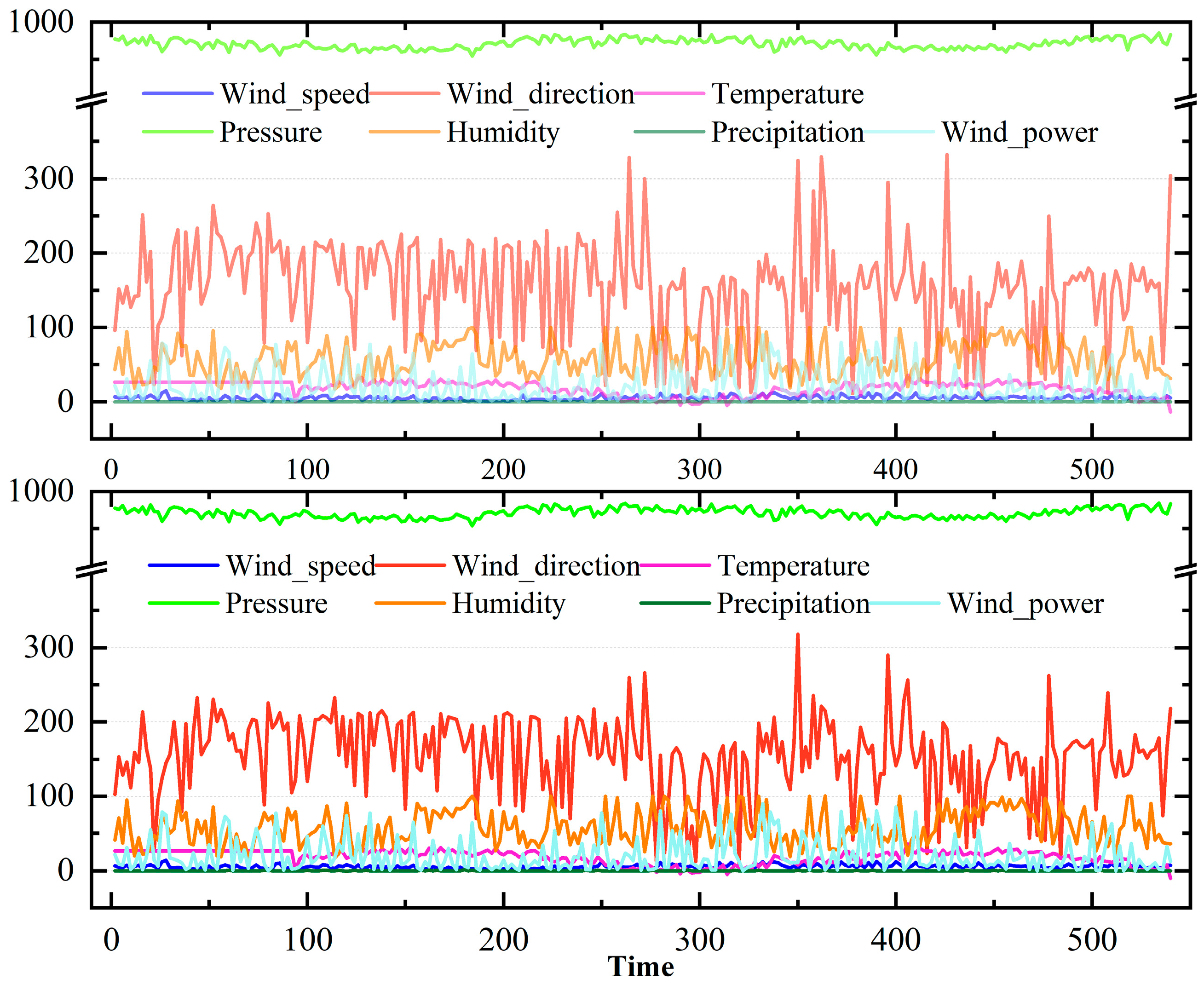
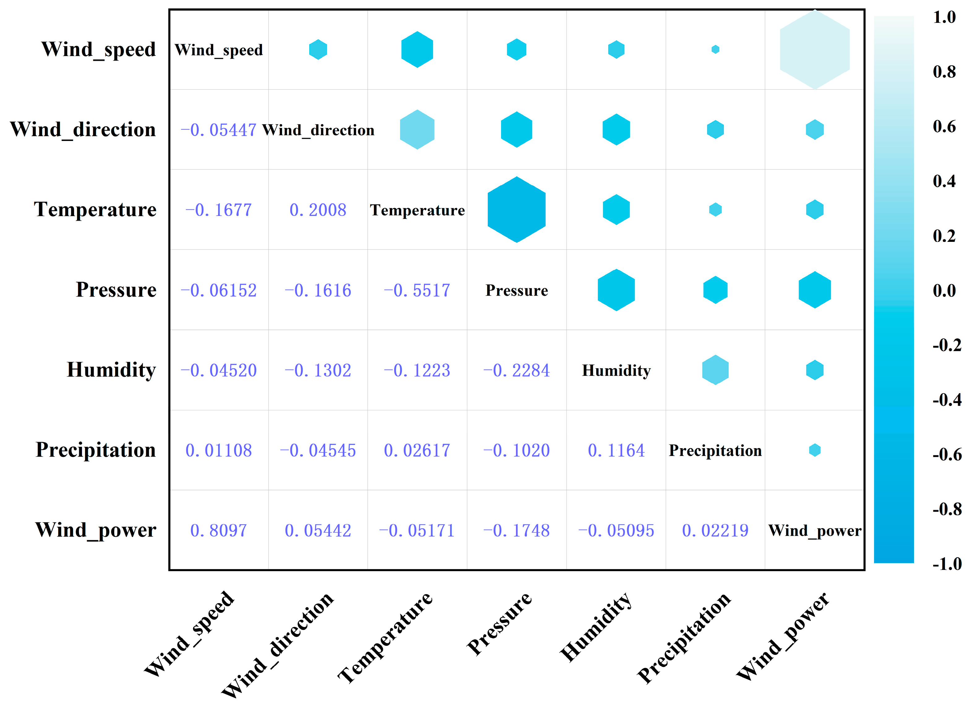
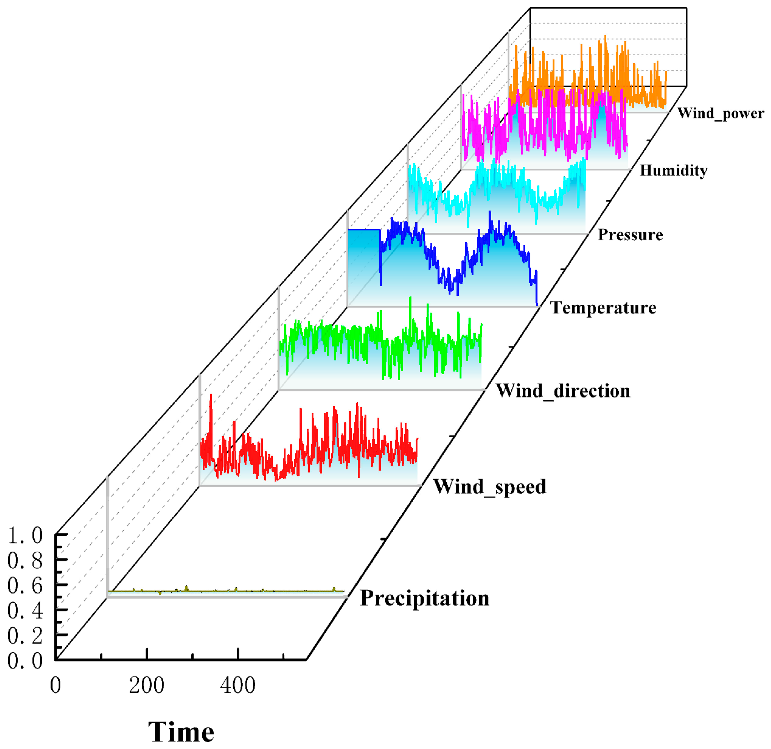
4.1. Data Description and Cleaning

The wind power data used in this study was obtained from a wind farm that operated from 1 January 2019 to 31 December 2020. The wind turbines in this farm have a height of 70 m and are rated at 1.5 kW. Data are recorded every 15 min resulting in a total of 70,094 data points with 96 entries recorded each day. Each data point includes information of the wind speed, the wind direction, the ambient temperature, the barometric pressure, the relative humidity, the rainfall, the actual power generated, and the recording status (normal or abnormal).

The anomalous data can have a negative impact on the convergence speed and the forecasting accuracy of the model. This study has cleaned up the raw wind power data as follows. (1) The data collected should be excluded during abnormal operating operation of the wind turbine. (2) It is necessary to exclude the data with wind speeds below the cut-in wind speed (3 m/s) and actual power equal to 0 (MW) to ensure a balanced distribution of data samples.

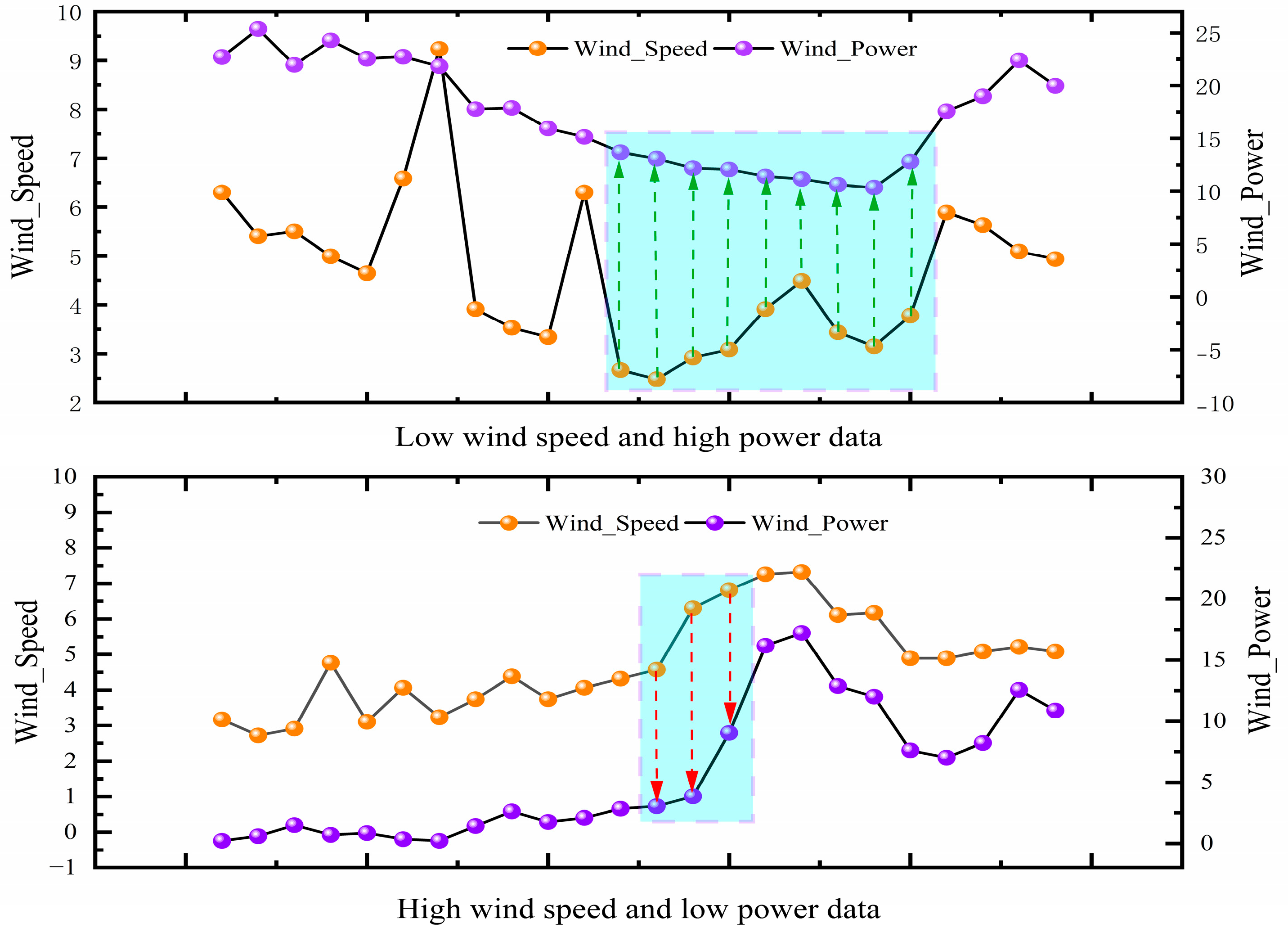
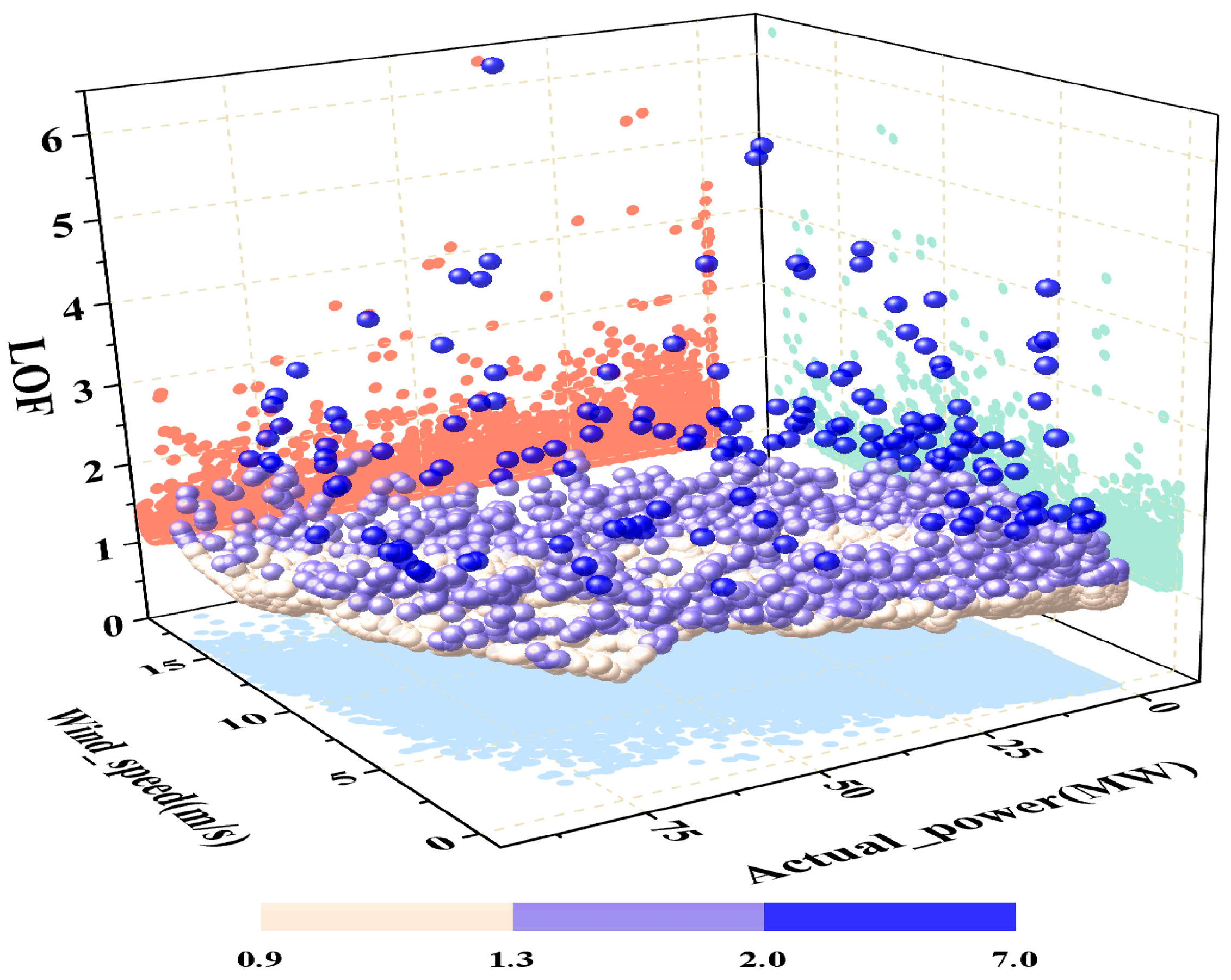
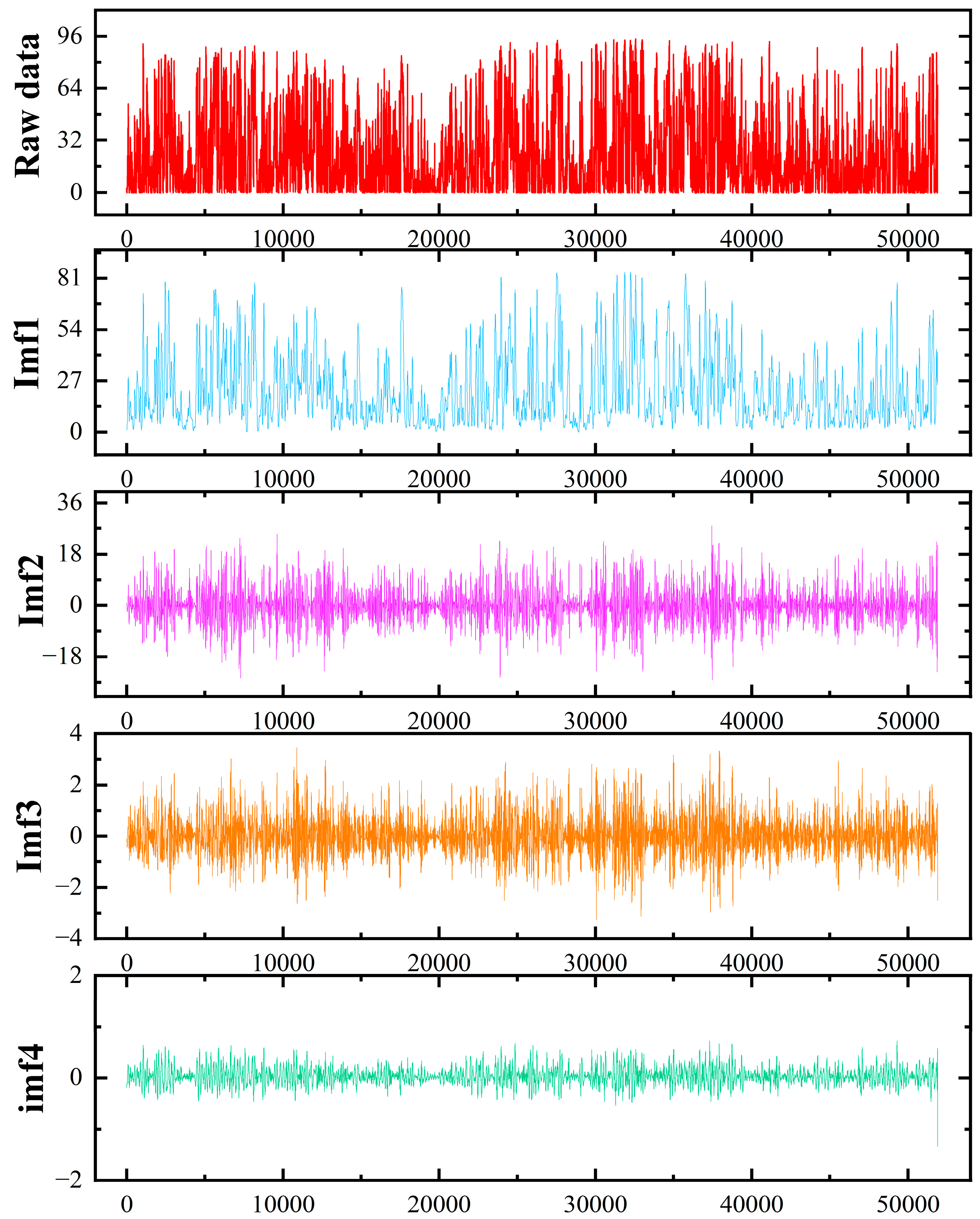
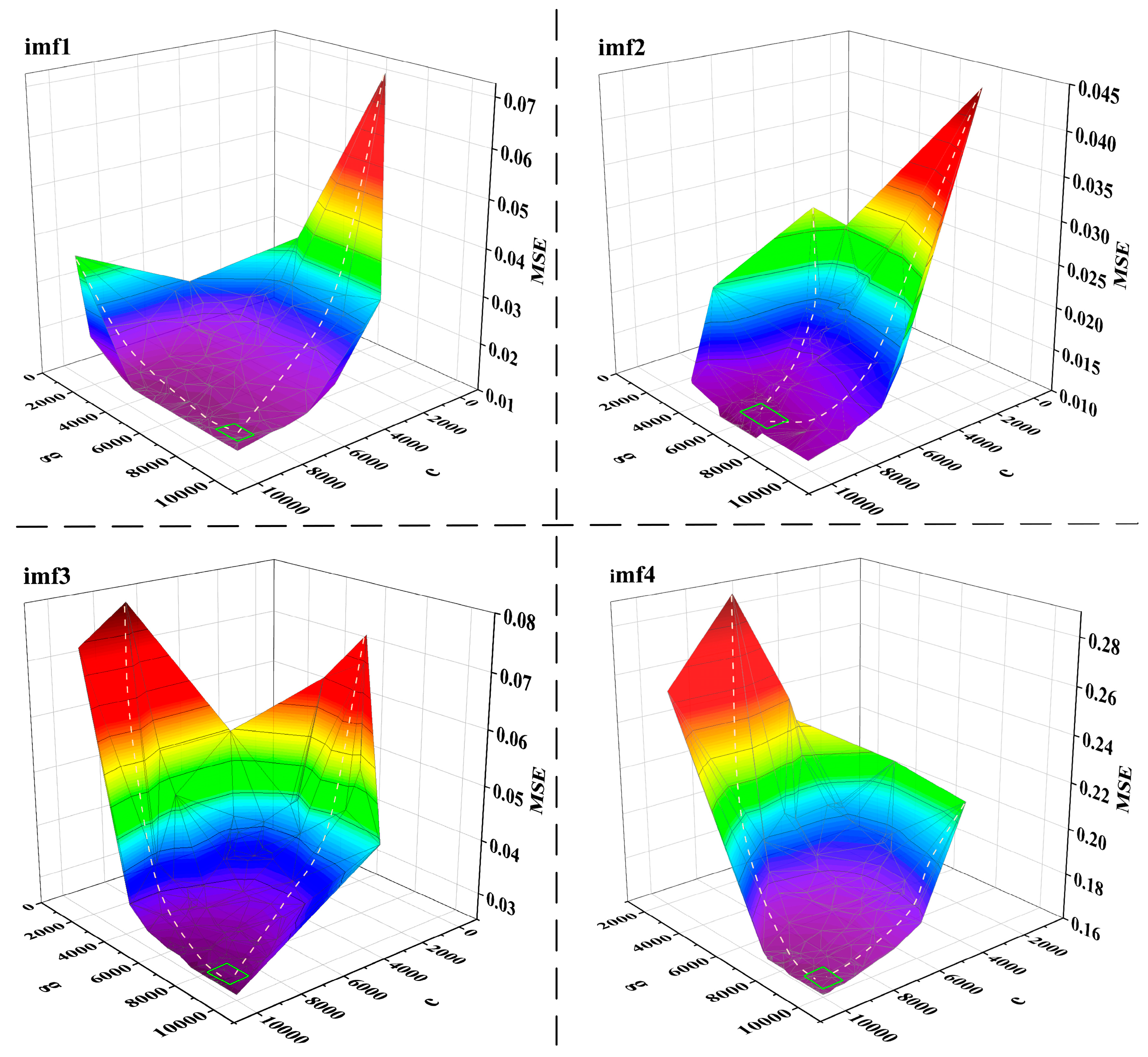
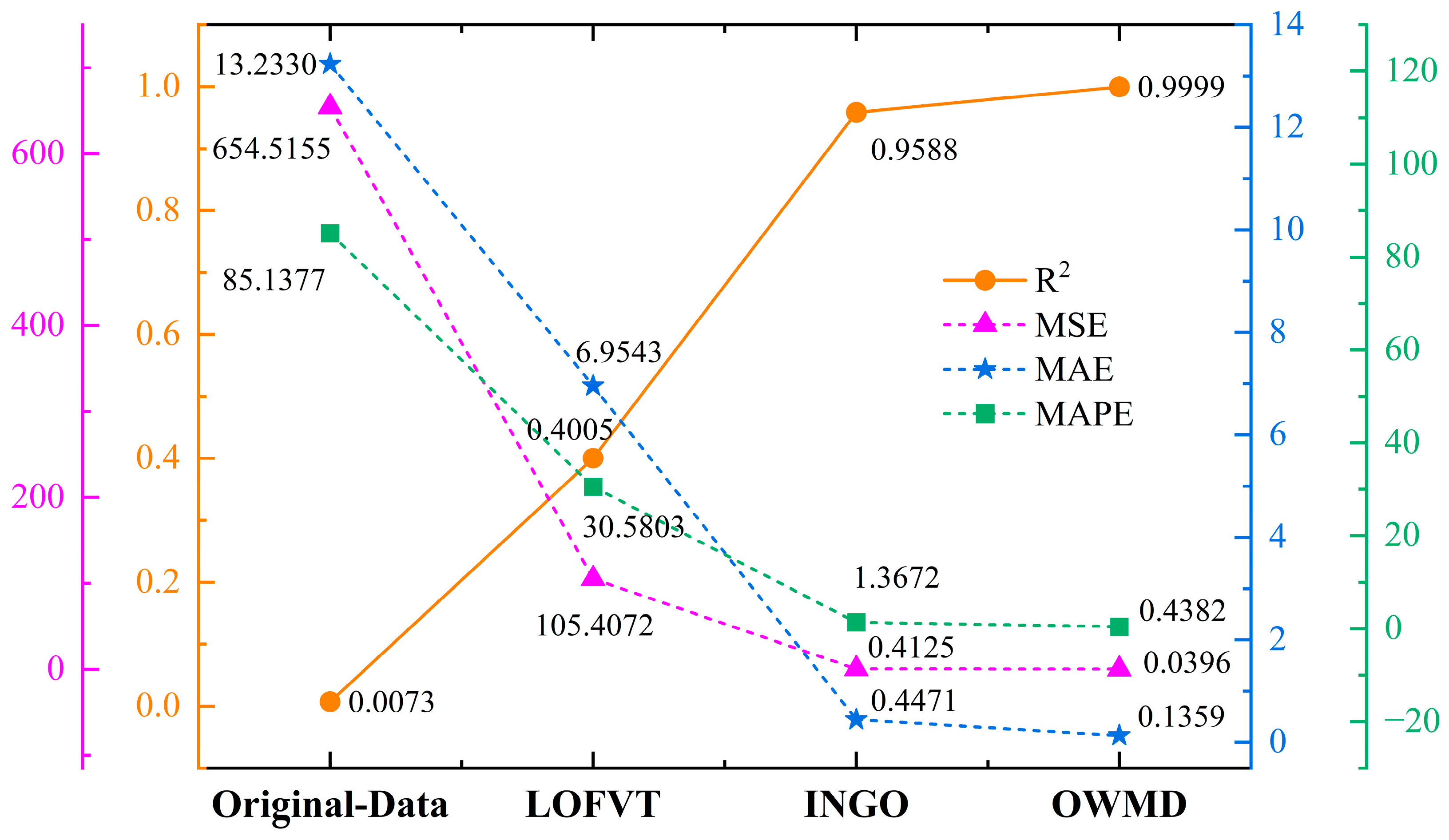
4.2. Experimental Results of Data Processing

The LOF algorithm was employed to screen the data during the data processing phase. The reasonable high wind speed low power and low wind speed high power data are retained in contrast to the approach of [29]. Figure 3 is the justification for the presence of the data due to inertia. Figure 4 shows the results of the wind power data screening process conducted in this study. The Savitzky–Golay filter was applied for smoothing to further reduce noise in the data. Figure 5 displays the data before and after smoothing.

Moreover, the wind power dataset contains numerous complex features, which can increase the model’s overall complexity. To address this issue, the Spearman coefficients [43] were computed to determine the inter-feature correlations, which are presented in Figure 6. Based on the inter-feature correlation analysis, the VT algorithm to classify the wind power data was employed with the classification results presented in

Table 2. VT model classification effect.

Season	Spring and Autumn		Summer		Winter
Weather	Cloudy and Rainy	Sunny	Cloudy and Rainy	Sunny	Cloudy and Rainy	Sunny
Amount	2349	879	3346	1516	1677	582
Logistic Regression	1903	44	2862	413	1288	413
Accuracy	81.01%	5.01%	85.53%	27.24%	76.80%	3.09%
SVC	2314	0	3341	0	1653	0
Accuracy	98.51%	0%	99.85%	0%	98.57%	0%
Random Forest	2349	879	3346	1516	1677	582
Accuracy	100%	100%	100%	100%	100%	100%

. The VT algorithm successfully divided the dataset into six sub-datasets with 100% accuracy. To account for the varying dimensions and units of the feature variables present in the wind power dataset, the data to minimize the impact of dimensional differences were normalized. Figure 7 illustrates the results of the L2 normalization procedure for the different data.

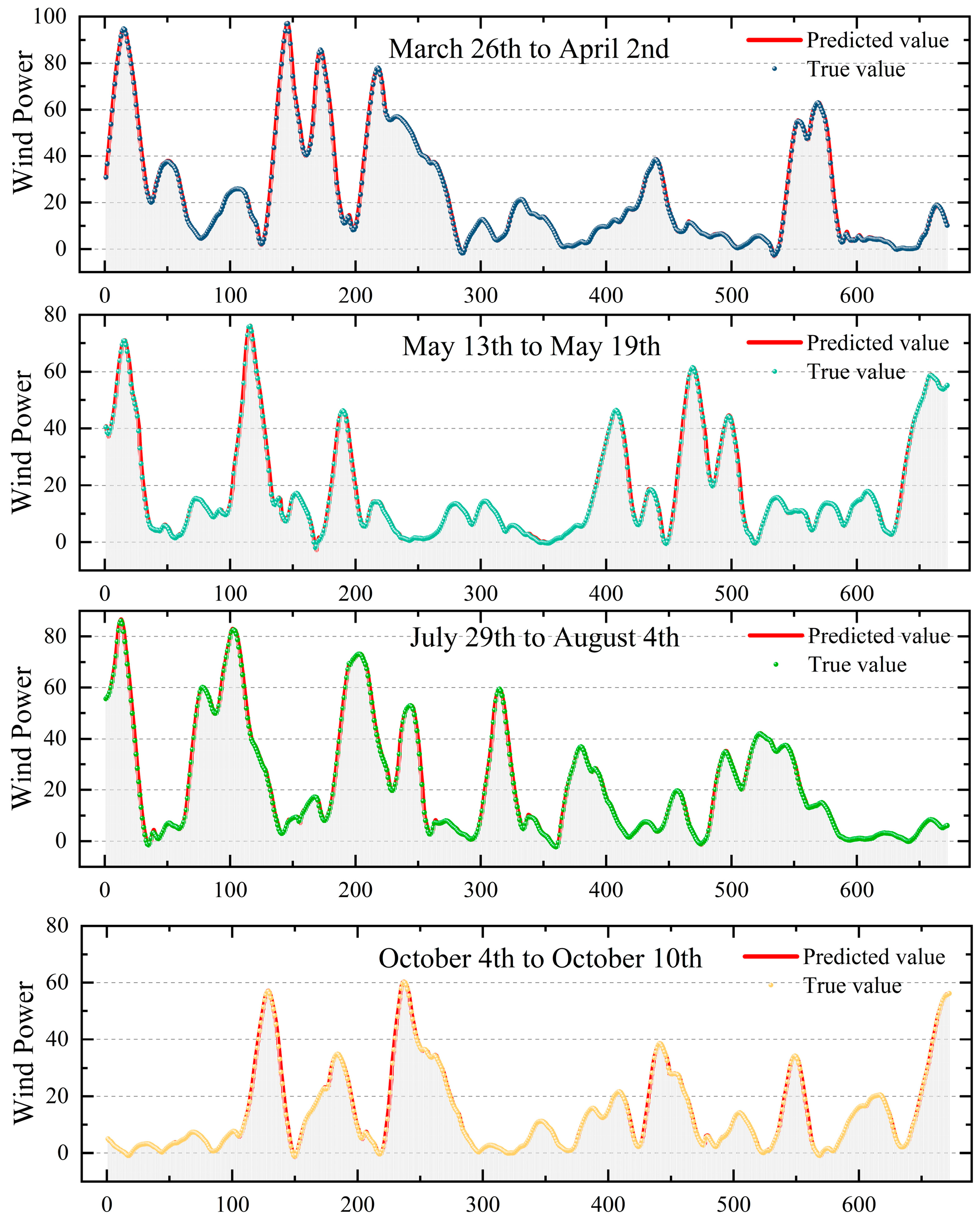
4.3. Testing and Analysis of Model Performance

To evaluate the prediction accuracy of the proposed model, the coefficient of determination, mean squared error, mean absolute error, and mean absolute percentage error as the evaluation indexes of the prediction model were used. The smaller the MSE, MAE, and MAPE values are, the better the accuracy and reliability of the proposed model have. The $R^2$ value reflects the interpretability of the model, where a value closer to 1 indicates stronger interpretability. The formulas for calculating these indicators are as follows:

$$R^2={\displaystyle \frac{{\sum }_{i=1}^N{\left(y_i-\overline{y_i}\right)}^2-{\sum }_{i=1}^N{\left(y_i-y_i^{\prime }\right)}^2}{{\sum }_{i=1}^N{\left(y_i-\overline{y_i}\right)}^2}}$$

(31)

$$MSE={\displaystyle \frac{1}{N}}\sum _{i=1}^N{\left(y_i-y_i^{\prime }\right)}^2$$

(32)

$$MAE={\displaystyle \frac{1}{N}}\sum _{i=1}^N\left|y_i-y_i^{\prime }\right|$$

(33)

$$MAPE={\displaystyle \frac{100\%}{N}}\sum _{i=1}^N\left|{\displaystyle \frac{y_i-y_i^{\prime }}{y_i}}\right|$$

(34)

where $y_i$ is the true value of wind power, $y_i^{\prime }$ is the predicted value of wind power, and $\overline{y_i}$is the average value of wind power.

After processing the wind power data, the INGO to optimize the hyperparameters of both VMD and LSSVR were utilized, respectively. The experimental results showed that the optimal minimum envelope entropy of VMD was obtained at k = 4 and α = 100. Figure 8 illustrates the effect of modal decomposition. The winter sunny weather dataset after classification contained relatively few data points. The optimization search process was swift and amenable to presentation as demonstrated in Figure 9.

Based on the above optimization process and the four evaluation indicators, the impact of each step in the proposed model on the accuracy of WPF was evaluated. The following models for comparison experiments were trained. (1) The original LSSVR model has not undergone any processing. (2) LOFVT-LSSVR is the model after data processing. (3) LOFVT-INGO-LSSVR is the LSSVR model after INGO optimization. (4) LOFVT-INGO-OVMD-LSSVR is the LSSVR model after OVMD modal decomposition. The training data used for comparison consisted of wind power data from the entirety of 2019 with a randomly selected test set of seven days taken from 2020. Specifically, the test set was comprised of data from 26 March to 2 April, 13 May to 19 May, 29 July to 4 August, and all wind power data from 4 October to 10 October 2020. For visual comparison, four time period prediction results from the proposed model across four seasons were randomly selected and displayed alongside the corresponding real power values in Figure 10. The average performance comparison results were presented in Figure 11.

It is clear that the model trained with raw data performed poorly with the lowest prediction accuracy from Figure 11. These results indicate that the raw data contains numerous outliers, noise and other sources of disturbance, which was unsuitable for direct use in training the model.

The comparison of the data-processed model with the original data prediction model shows significant improvements. The average MSE, average MAE, and average MAPE of the data-processed model predictions decreased by 540.1083, 6.2787, and 54.5534, respectively. The average R² increased by 0.3932. These results demonstrated that the data screening, data smoothing, and data normalization techniques proposed in this study can effectively improve the availability of wind power data, which can enhance the prediction accuracy of the LSSVR model.

The INGO algorithm was utilized to optimize the parameters for each sub-prediction model resulting in significant improvements in prediction accuracy. The $c$ and $g$ of LSSVR are critical parameters, which strongly influence the accuracy of the prediction models. The OWMD algorithm was used to perform serial decomposition on the wind power data in order to explore the time-frequency relationships between different features. The average values of MSE, MAE, and MAPE for the forecast results decreased to 0.0396, 0.1359, and 0.4382, respectively. The average R² value increased to 0.9999, which validated the effectiveness of OVMD in predicting wind power.

4.4. Analysis of the Effect of Time Duration

To investigate the effect of the historical wind power data duration on the accuracy and stability of the proposed model, four historical prediction duration experiments were conducted. These experiments used the first 12 moments (3 h), the first 6 moments (1.5 h), the first 3 moments (45 min), and the first 2 moments (30 min) to predict the wind power at the last 1 moment (15 min). These experimental results are shown in

Table 3. The effect of model prediction duration on prediction results.

Predicted Moments	Cloudy–Rainy (Spring–Autumn) 1				Sunny (Spring–Autumn) 2
	R2	MSE	MAE	MAPE	R2	MSE	MAE	MAPE
12	0.9998	0.0284	0.1213	0.3793	0.9997	0.0500	0.1665	0.4890
6	0.9998	0.0264	0.1158	0.3682	0.9998	0.0425	0.1515	0.4294
3	0.9998	0.0244	0.1073	0.3587	0.9998	0.0438	0.1505	0.4473
2	0.9998	0.0300	0.1197	0.3948	0.9997	0.0526	0.1673	0.4758
	Cloudy–Rainy (Summer) 3				Sunny (Summer) 4
	R2	MSE	MAE	MAPE	R2	MSE	MAE	MAPE
12	0.9973	0.7069	0.2777	1.1421	0.9996	0.0424	0.1465	0.4928
6	0.9978	0.5700	0.2601	1.0407	0.9998	0.0434	0.1409	0.4796
3	0.9987	0.3287	0.2072	0.7508	0.9999	0.0395	0.1329	0.4579
2	0.9994	0.2225	0.1903	0.6034	0.9998	0.0505	0.1498	0.5185
	Cloudy–Rainy (Winter) 5				Sunny (Winter) 6
	R2	MSE	MAE	MAPE	R2	MSE	MAE	MAPE
12	0.9997	0.0604	0.1617	0.4720	0.9998	0.0905	0.2203	0.5795
6	0.9997	0.0448	0.1469	0.4311	0.9998	0.0771	0.1922	0.5089
3	0.9997	0.0424	0.1379	0.4167	0.9999	0.0674	0.1746	0.5070
2	0.9997	0.0531	0.1548	0.4768	0.9998	0.0849	0.2005	0.5356

.

The best prediction results were achieved in the cloudy–rainy (spring–autumn) model, the sunny (summer) model, the cloudy–rainy (winter) model, and the sunny (winter) for the first 3 moments (i.e., the first 45 min). Utilizing longer historical forecast data can lead to an increase in the amount of erratic or unpredictable data, which may reduce the accuracy of WPF. Conversely, shorter historical forecast data may not have sufficient data features to accurately reflect the characteristics of local wind power patterns, which also leads to decreased prediction accuracy.

The sunny (spring–autumn) model yielded the most accurate wind power when using the first 6 moments (i.e., first 1.5 h). Based on the analysis, the random fluctuations of primary influencing factors appeared. The wind speed during sunny days in the spring and autumn is relatively reduced, which decreases the overall uncertainty of the forecast. Therefore, utilizing longer historical forecast data may potentially increase the accuracy of wind power. The best prediction results were obtained only by using the first 2 moments (i.e., the first 30 min) in the cloudy–rainy (summer) model. It can be seen that the random fluctuations of primary influencing factors during cloudy and rainy days in summer and the wind speed tended to increase. As a result, utilizing longer historical forecast data may lead to an increase in abrupt changes within the data, which can make it challenging for the model to accurately predict wind power patterns. Conversely, utilizing shorter historical forecast data may reduce the impact of abrupt changes, which leads to more accurate predictions. Overall, the time analysis of the different wind power sub-models highlighted the importance of classifying data based on specific seasonal and weather conditions. Targeted training of the data for each category can help to optimize the accuracy of wind power during different weather patterns.

4.5. Comparative Analysis of the Performance of Different Models

To validate the prediction performance of the proposed model, the wind power dataset from 2019 to 2020 as the sample was used. Pre-processed and classified the dataset into six sub-datasets and then compared the prediction performance of different models for these sub-datasets.

For each sub-dataset, RF, SVM, backpropagation (BP), LSTM [44], GRU, BiLSTM, VMD-CNN-GRU [45], and EEMD-Tent-ISSA-LSSVM [46] were trained. These models were used to predict the wind power for the next moment [47,48,49]. These eight prediction models were selected from traditional machine learning models, deep learning time series models, and hybrid machine learning models, which are representative. The specific prediction results are presented in

Table 4. Performance comparison of different wind power forecasting models.

Model	Cloudy–Rainy (Spring–Autumn) 1				Sunny (Spring–Autumn) 2
	R2	MSE	MAE	MAPE	R2	MSE	MAE	MAPE
RF	0.9642	12.6803	2.3702	1.1204	0.9447	24.8045	3.3552	2.4979
SVM	0.9723	9.8112	2.0545	0.9328	0.9544	20.4520	2.9548	2.1315
BP	0.9737	9.3282	2.1182	1.4274	0.9567	19.3965	3.0852	3.5038
LSTM	0.9708	10.3681	2.1875	1.3118	0.9618	17.1685	2.7071	2.9555
GRU	0.9770	8.1756	2.0697	1.4930	0.9671	14.7880	2.6527	3.6855
BiLSTM	0.9733	9.4630	2.0714	1.2465	0.9651	15.6774	2.7597	4.1799
VMD-CNN-GRU	0.9839	5.7166	1.6152	0.8507	0.9859	6.3392	1.7496	0.8820
EEMD-Tent-ISSA-LSSVM	0.9947	1.8755	0.9311	0.7243	0.9917	3.7271	1.4983	1.1071
This study	0.9998	0.0244	0.1073	0.3587	0.9998	0.0425	0.1515	0.4294
	Cloudy–Rainy (Summer) 3				Sunny (Summer) 4
	R2	MSE	MAE	MAPE	R2	MSE	MAE	MAPE
RF	0.9565	13.5186	2.3189	1.1105	0.9397	26.4657	3.2104	1.4290
SVM	0.9674	10.1306	2.0274	1.1489	0.9457	22.7681	2.9666	1.0941
BP	0.9695	9.4569	2.0355	0.9290	0.9539	19.3426	2.9034	1.3445
LSTM	0.9644	11.0549	2.2376	1.5858	0.9618	16.0321	2.6734	1.1414
GRU	0.9671	10.2121	2.1687	1.1958	0.9666	14.0147	2.4278	0.8392
BiLSTM	0.9649	10.8831	2.2691	1.4837	0.9626	15.6901	2.5952	0.9851
VMD-CNN-GRU	0.9914	2.6783	1.0699	0.6762	0.9698	12.6618	2.5256	1.3718
EEMD-Tent-ISSA-LSSVM	0.9952	1.4734	0.8747	0.6391	0.9939	2.5483	1.1099	0.6022
This study	0.9994	0.2225	0.1903	0.6034	0.9999	0.0395	0.1329	0.4579
	Cloudy–Rainy (Winter) 5				Sunny (Winter) 6
	R2	MSE	MAE	MAPE	R2	MSE	MAE	MAPE
RF	0.9443	26.8113	3.0183	1.1126	0.9457	29.2208	3.4596	1.7838
SVM	0.9448	26.6055	2.9256	1.0871	0.9444	29.8866	3.4573	2.4774
BP	0.9605	19.0411	2.7824	1.8197	0.9494	27.1994	3.4152	2.9089
LSTM	0.9533	22.4837	2.8158	1.8817	0.9531	25.2925	3.3272	2.5044
GRU	0.9620	18.3114	2.4565	0.8655	0.9541	24.7380	2.3252	2.6394
BiLSTM	0.9505	23.8340	2.7814	1.0198	0.9568	23.2750	3.2884	2.6072
VMD-CNN-GRU	0.9809	9.1978	1.9237	0.7960	0.9846	8.3161	1.9797	1.4777
EEMD-Tent-ISSA-LSSVM	0.9930	3.3692	1.1673	1.2333	0.9927	3.9321	1.3815	1.4261
This study	0.9997	0.0424	0.1379	0.4167	0.9999	0.0674	0.1746	0.5070

and the average results for each model are shown in Figure 12.

As given in Table 3 and Figure 12, the hybrid prediction model has significantly improved the model prediction accuracy compared to the traditional machine learning and deep learning prediction models. The VMD-CNN-GRU hybrid deep learning prediction model showed an average R² of 0.9828. The average MSE, MAE, and MAPE are 7.4850, 1.8106, and 1.0091, respectively. The EEMD-Tent-ISSA-LSSVM hybrid machine learning model further enhanced the prediction accuracy with an average R² of 0.9935. The average MSE, MAE, and MAPE decreased to 2.8209, 1.8209, and 1.0091, respectively. Notably, the proposed LOFVT-INGO-OVMD-LSSVR model achieved the best prediction results among the six sub-models, with an average R² of 0.9998 and low values for average MSE, MAE, and MAPE (0.0244, 0.1073, and 0.3587, respectively). The hybrid prediction model demonstrated superior performance in accurately predicting wind power, while the proposed LOFVT-INGO-OVMD-LSSVR model exhibited high accuracy and reliability.

5. Conclusions

The accurate forecasting of wind power is essential for ensuring reliable power dispatch and system planning for the grid. This study proposes a new hybrid model of LOFVT-INGO-OVMD-LSSVR for ultra-short-term WPF. The research conclusion is as follows:

(1)

The proposed model can accurately forecast the power production of large wind power plants up to 15 min in advance. The experimental results show that the proposed model has an average R² of 0.9998.

(2)

The average MSE, average MAE, and average MAPE are as low as 0.0244, 0.1073, and 0.3587, which displayed the best results in ultra-short-term WPF. This model provided a reliable method for stable operation, planning, and maintenance of wind power plants, which offers robust support for the continued development of clean energy and energy distribution planning.

References

1. Wu, Z.; Zeng, S.; Jiang, R.; Zhang, H.; Yang, Z. Explainable temporal dependence in multi-step wind power forecast via decomposition based chain echo state networks. Energy 2023, 270, 126906. [Google Scholar] [CrossRef]
2. Cui, Y.; Chen, Z.; He, Y.; Xiong, X.; Li, F. An algorithm for forecasting day-ahead wind power via novel long short-term memory and wind power ramp events. Energy 2023, 263, 125888. [Google Scholar] [CrossRef]
3. Dai, X.; Liu, G.-P.; Hu, W. An online-learning-enabled self-attention-based model for ultra-short-term wind power forecasting. Energy 2023, 272, 127173. [Google Scholar] [CrossRef]
4. Liu, H.; Zhang, Z. A bilateral branch learning paradigm for short term wind power prediction with data of multiple sampling resolutions. J. Clean. Prod. 2022, 380, 134977. [Google Scholar] [CrossRef]
5. Shi, J.; Wang, B.; Luo, K.; Wu, Y.; Zhou, M.; Watada, J. Ultra-short-term wind power interval prediction based on multi-task learning and generative critic networks. Energy 2023, 272, 127116. [Google Scholar] [CrossRef]
6. Wang, Q.; Luo, K.; Wu, C.; Tan, J.; He, R.; Ye, S.; Fan, J. Inter-farm cluster interaction of the operational and planned offshore wind power base. J. Clean. Prod. 2023, 396, 136529. [Google Scholar] [CrossRef]
7. Marčiukaitis, M.; Žutautaitė, I.; Martišauskas, L.; Jokšas, B.; Gecevičius, G.; Sfetsos, A. Non-linear regression model for wind turbine power curve. Renew. Energy 2017, 113, 732–741. [Google Scholar] [CrossRef]
8. Chen, H.; Birkelund, Y.; Zhang, Q. Data-augmented sequential deep learning for wind power forecasting. Energy Convers. Manag. 2021, 248, 114790. [Google Scholar] [CrossRef]
9. Li, L.; Li, Y.; Zhou, B.; Wu, Q.; Shen, X.; Liu, H.; Gong, Z. An adaptive time-resolution method for ultra-short-term wind power prediction. Int. J. Electr. Power Energy Syst. 2020, 118, 105814. [Google Scholar] [CrossRef]
10. Wang, H.; Ye, J.; Huang, L.; Wang, Q.; Zhang, H. A multivariable hybrid prediction model of offshore wind power based on multi-stage optimization and reconstruction prediction. Energy 2023, 262, 125428. [Google Scholar] [CrossRef]
11. Jin, H.; Li, Y.; Wang, B.; Yang, B.; Jin, H.; Cao, Y. Adaptive forecasting of wind power based on selective ensemble of offline global and online local learning. Energy Convers. Manag. 2022, 271, 116296. [Google Scholar] [CrossRef]
12. Jørgensen, K.L.; Shaker, H.R. Wind Power Forecasting Using Machine Learning: State of the Art, Trends and Challenges. In Proceedings of the 2020 IEEE 8th International Conference on Smart Energy Grid Engineering (SEGE), Oshawa, ON, Canada, 12–14 August 2020; pp. 44–50. [Google Scholar] [CrossRef]
13. Heinermann, J.; Kramer, O. Machine learning ensembles for wind power prediction. Renew. Energy 2016, 89, 671–679. [Google Scholar] [CrossRef]
14. Demolli, H.; Dokuz, A.S.; Ecemis, A.; Gokcek, M. Wind power forecasting based on daily wind speed data using machine learning algorithms. Energy Convers. Manag. 2019, 198, 111823. [Google Scholar] [CrossRef]
15. Lu, P.; Ye, L.; Zhong, W.; Qu, Y.; Zhai, B.; Tang, Y.; Zhao, Y. A novel spatio-temporal wind power forecasting framework based on multi-output support vector machine and optimization strategy. J. Clean. Prod. 2020, 254, 119993. [Google Scholar] [CrossRef]
16. Wen, S.; Li, Y.; Su, Y. A new hybrid model for power forecasting of a wind farm using spatial–temporal correlations. Renew. Energy 2022, 198, 155–168. [Google Scholar] [CrossRef]
17. Chen, C.; Liu, H. Medium-term wind power forecasting based on multi-resolution multi-learner ensemble and adaptive model selection. Energy Convers. Manag. 2020, 206, 112492. [Google Scholar] [CrossRef]
18. Jalali, S.M.J.; Ahmadian, S.; Khodayar, M.; Khosravi, A.; Shafie-khah, M.; Nahavandi, S.; Catalao, J.P. An advanced short-term wind power forecasting framework based on the optimized deep neural network models. Int. J. Electr. Power Energy Syst. 2022, 141, 108143. [Google Scholar] [CrossRef]
19. Yu, C.; Li, Y.; Zhang, M. An improved Wavelet Transform using Singular Spectrum Analysis for wind speed forecasting based on Elman Neural Network. Energy Convers. Manag. 2017, 148, 895–904. [Google Scholar] [CrossRef]
20. Wang, J.; Zhu, H.; Zhang, Y.; Cheng, F.; Zhou, C. A novel prediction model for wind power based on improved long short-term memory neural network. Energy 2023, 265, 126283. [Google Scholar] [CrossRef]
21. Xiao, Y.; Zou, C.; Chi, H.; Fang, R. Boosted GRU model for short-term forecasting of wind power with feature-weighted principal component analysis. Energy 2023, 267, 126503. [Google Scholar] [CrossRef]
22. Wang, J.; Heng, J.; Xiao, L.; Wang, C. Research and application of a combined model based on multi-objective optimization for multi-step ahead wind speed forecasting. Energy 2017, 125, 591–613. [Google Scholar] [CrossRef]
23. Naik, J.; Satapathy, P.; Dash, P.K. Short-term wind speed and wind power prediction using hybrid empirical mode decomposition and kernel ridge regression. Appl. Soft Comput. 2018, 70, 1167–1188. [Google Scholar] [CrossRef]
24. Wang, D.; Luo, H.; Grunder, O.; Lin, Y. Multi-step ahead wind speed forecasting using an improved wavelet neural network combining variational mode decomposition and phase space reconstruction. Renew. Energy 2017, 113, 1345–1358. [Google Scholar] [CrossRef]
25. Wei, J.; Wu, X.; Yang, T.; Jiao, R. Ultra-short-term forecasting of wind power based on multi-task learning and LSTM. Int. J. Electr. Power Energy Syst. 2023, 149, 109073. [Google Scholar] [CrossRef]
26. Lu, P.; Ye, L.; Tang, Y.; Zhao, Y.; Zhong, W.; Qu, Y.; Zhai, B. Ultra-short-term combined prediction approach based on kernel function switch mechanism. Renew. Energy 2021, 164, 842–866. [Google Scholar] [CrossRef]
27. Niu, D.; Sun, L.; Yu, M.; Wang, K. Point and interval forecasting of ultra-short-term wind power based on a data-driven method and hybrid deep learning model. Energy 2022, 254, 124384. [Google Scholar] [CrossRef]
28. Yu, M.; Niu, D.; Gao, T.; Wang, K.; Sun, L.; Li, M.; Xu, X. A novel framework for ultra-short-term interval wind power prediction based on RF-WOA-VMD and BiGRU optimized by the attention mechanism. Energy 2023, 269, 126738. [Google Scholar] [CrossRef]
29. Liu, L.; Liu, J.; Ye, Y.; Liu, H.; Chen, K.; Li, D.; Dong, X.; Sun, M. Ultra-short-term wind power forecasting based on deep Bayesian model with uncertainty. Renew. Energy 2023, 205, 598–607. [Google Scholar] [CrossRef]
30. Breunig, M.M.; Kriegel, H.-P.; Ng, R.T.; Sander, J. LOF: Identifying density-based local outliers. In Proceedings of the 2000 ACM SIGMOD International Conference on Management of Data, Dallas, TX, USA, 16–18 May 2000; ACM: New York, NY, USA, 2000; pp. 93–104. [Google Scholar] [CrossRef]
31. Gorry, P.A. General least-squares smoothing and differentiation by the convolution (Savitzky-Golay) method. Anal. Chem. 1990, 62, 570–573. [Google Scholar] [CrossRef]
32. Ho, T.K. The random subspace method for constructing decision forests. IEEE Trans. Pattern. Anal. Mach. Intell. 1998, 20, 832–844. [Google Scholar] [CrossRef]
33. Cox, D.R. The Regression Analysis of Binary Sequences. J. R. Stat. Soc. Ser. B Methodol. 1958, 20, 215–232. [Google Scholar] [CrossRef]
34. Breiman, L. Random Forests. Mach. Learn. 2001, 45, 5–32. [Google Scholar] [CrossRef]
35. Cortes, C.; Vapnik, V. Support-vector networks. Mach. Learn. 1995, 20, 273–297. [Google Scholar]
36. Dehghani, M.; Hubálovský, Š.; Trojovský, P. Northern Goshawk Optimization: A New Swarm-Based Algorithm for Solving Optimization Problems. IEEE Access 2021, 9, 162059–162080. [Google Scholar] [CrossRef]
37. Jiang, H.; Kwong, C.K.; Chen, Z.; Ysim, Y.C. Chaos particle swarm optimization and T–S fuzzy modeling approaches to constrained predictive control. Expert Syst. Appl. 2012, 39, 194–201. [Google Scholar] [CrossRef]
38. Dragomiretskiy, K.; Zosso, D. Variational Mode Decomposition. IEEE Trans. Signal Process. 2014, 62, 531–544. [Google Scholar] [CrossRef]
39. Suykens, J.A.; Vandewalle, J. Least squares support vector machine classifiers. Neural Process. Lett. 1999, 9, 293–300. [Google Scholar]
40. Wu, X.; Ye, Q. Fault diagnosis and prognostic of solid oxide fuel cells. J. Power Sources 2016, 321, 47–56. [Google Scholar] [CrossRef]
41. Ghaedi, M.; Rahimi M reza Ghaedi, A.M.; Tyagi, I.; Agarwal, S.; Gupta, V.K. Application of least squares support vector regression and linear multiple regression for modeling removal of methyl orange onto tin oxide nanoparticles loaded on activated carbon and activated carbon prepared from Pistacia atlantica wood. J. Colloid Interface Sci. 2016, 461, 425–434. [Google Scholar] [CrossRef]
42. Goyal, M.K.; Bharti, B.; Quilty, J.; Adamowski, J.; Pandey, A. Modeling of daily pan evaporation in sub tropical climates using ANN, LS-SVR, Fuzzy Logic, and ANFIS. Expert Syst. Appl. 2014, 41, 5267–5276. [Google Scholar] [CrossRef]
43. Spearman, C. The Proof and Measurement of Association Between Two Things; American Psychological Association (APA): Washington, DC, USA, 1961. [Google Scholar]
44. Mohamed, M.; Gharib, M. PAM: Cultivate a Novel LSTM Predictive analysis Model for The Behavior of Cryptocurrencies. Sustain. Mach. Intell. J. 2024, 6, 1–10. [Google Scholar] [CrossRef]
45. Zhao, Z.; Yun, S.; Jia, L.; Guo, J.; Meng, Y.; He, N.; Li, X.; Shi, J.; Yang, L. Hybrid VMD-CNN-GRU-based model for short-term forecasting of wind power considering spatio-temporal features. Eng. Appl. Artif. Intell. 2023, 121, 105982. [Google Scholar] [CrossRef]
46. Li, Z.; Luo, X.; Liu, M.; Cao, X.; Du, S.; Sun, H. Wind power prediction based on EEMD-Tent-SSA-LS-SVM. Energy Rep. 2022, 8, 3234–3243. [Google Scholar] [CrossRef]
47. Abouhawwash, M.; Jameel, M.; Askar, S.S. Machine intelligence framework for predictive modeling of CO2 concentration: A path to sustainable environmental management. Sustain. Mach. Intell. J. 2023, 2, 1–8. [Google Scholar] [CrossRef]
48. El-Shahat, D.; Tolba, A. A Hybridized CNN-LSTM-MLP-KNN Model for Short-Term Solar Irradiance Forecasting. Sustain. Mach. Intell. J. 2025, 10, 1–22. [Google Scholar] [CrossRef]
49. Metwaly, A.A.; Elhenawy, I. Predictive Intelligence Technique for Short-Term Load Forecasting in Sustainable Energy Grids. Sustain. Mach. Intell. J. 2023, 5, 1–7. [Google Scholar] [CrossRef]
Figure 1. The structure of LSSVR.
Energies 18 01849 g001
Figure 2. Flowchart of the LOFVT-INGO-OVMD-LSSVR model.
Energies 18 01849 g002
Figure 3. Reasonable data for wind power (reasonable high wind speed low power, low wind speed high power data in blue boxes).
Energies 18 01849 g003
Figure 4. LOF detection effect (dark blue data points are abnormal data, light blue data points are reasonable data, gray data points are normal data).
Energies 18 01849 g004
Figure 5. Data smoothing effect (the above figure is the data before smoothing, the following figure is the data after smoothing).
Energies 18 01849 g005
Figure 6. Correlation between different feature data.
Energies 18 01849 g006
Figure 7. Data normalization process.
Energies 18 01849 g007
Figure 8. Modal decomposition effect ( k = 4 ,   α = 100 ).
Energies 18 01849 g008
Figure 9. LSSVR model optimization search process.
Energies 18 01849 g009
Figure 10. Test set final prediction results.
Energies 18 01849 g010
Figure 11. Average effect of different modules on the model in the test set.
Energies 18 01849 g011
Figure 12. Comparison of average model performance.
Energies 18 01849 g012