Abstract
Highlighting the importance of artificial intelligence and machine learning approaches in engineering and fluid mechanics problems, especially in heat transfer applications is main goal of the presented article. With the advancement in Artificial Intelligence (AI) and Machine Learning (ML) techniques, the computational efficiency and accuracy of numerical results are enhanced. The theme of the study is to use machine learning techniques to examine the thermal analysis of MHD boundary layer flow of Eyring-Powell Hybrid Nanofluid (EPHNFs) passing a horizontal cylinder embedded in a porous medium with heat source/sink and viscous dissipation effects. The considered base fluid is water () and hybrid nanoparticles titanium oxide () and Copper oxide (). The governing flow equations are nonlinear PDEs. Non-similar system of PDEs are obtained with efficient conversion variables. The dimensionless PDEs are truncated using a local non-similarity approach up to third level and numerical solution is evaluated using MATLAB built-in-function bvp4c. Artificial Neural Networks (ANNs) simulation approach is used to trained the networks to predict the solution behavior. Thermal boundary layer improves with the enhancement in the value of . The accuracy and reliability of ANNs predicted solution is addressed with computation of correlation index and residual analysis. The RMSE is evaluated [0.04892, 0.0007597, 0.0007596, 0.01546, 0.008871, 0.01686] for various scenarios. It is observed that when concentration of hybrid nanoparticles increases then thermal characteristics of the Eyring-Powell Hybrid Nanofluid (EPHNFs) passing a horizontal cylinder.
1. Introduction
The Eyring-Powell fluid model is a significant non-Newtonian fluid model developed to address the limitations of classical Newtonian and non-Newtonian models in representing real fluid behavior. Based on statistical mechanics and inspired by the Eyring theory of reaction rates, it provides a more accurate description of viscosity variations with shear rate changes. This model is particularly useful in applications involving shear-thinning behavior without the singularity issues of power-law fluids. Unlike the Casson model, the Eyring-Powell model does not require a yield stress to initiate flow. This model is used widely in industries that involve lubricants, polymer processing, and biological fluids, including blood flow in larger arteries. The effects of DuFour and Soret on boundary layer flow of Eyring-Powell nanofluid over a cylinder with viscous dissipation effects were analyzed [1]. They used non-similarity solution with bvp4c MATLAB R2017b built in function to evaluate numerically solution of the considered problem. The effects of thermal radiation and thermal conductivity variation on chemically reactive, free convective Powell-Eyring nanofluid flow around a cylinder were analyzed theoretically [2]. Furthermore, heat transfer in Eyring-Powell fluids has been explored in different settings, including MHD systems with viscous dissipation [3], fluid flow inside a pipe [4], oscillatory flow in a porous channel with energy-dependent viscosity [5], and radiative and chemically reactive flows incorporating non-Fourier heat flux and non-Fick mass flux theories [6].
Gaffar et. al. [7] investigated numerical solution of MHD boundary layer flow of tangent hyperbolic fluid over a cylinder using implicit finite difference scheme known as Keller Box method. The effects of ternary nanoparticles i.e., titanium oxide, silicon oxide and aluminum oxide (TiO2–SiO2–Al2O3) on boundary layer flow of non-Newtonian model was examined by Turabi et al. [8]. They investigated that the increasing nature of viscous dissipation effects results in the improvement of thermal boundary layer. According to their investigation, thermal boundary layer improves as viscous dissipation effects upsurge. Convective heat transport analysis of non-Newtonian nanofluid with two-layer viscous dissipative effects in a channel was studied by Amin et al. [9]. Das et al. [10] investigated dynamical behavior of MHD boundary layer flow of hybrid nanofluid in a gyrating channel. The hydrodynamic nature of MHD gyrating stream of hybrid nanofluid flow of non-Newtonian model were addressed in a vertical plate [11]. They concluded that presence of Coriolis and Lorentz forces with Hall currents significantly alters the fluid motion. Das et al. [12] scrutinized hydro-thermal dynamics of magnetized rotational non-Newtonian hybrid nanofluid. There is a lot of literature is available to explore the fascinating phenomena of hybrid nanoparticles and non-Newtonian fluid [13,14,15,16,17]. Saeed et al. [18] explored the effects of hybrid nanoparticles on MHD boundary layer flow with couple stress. Shoaib and Javed [19] examined sensitivity of convective boundary layer flow nanofluid with non-isothermal condition. Amin et al. [20] inspected MHD impact on boundary layer flow of nanofluid in a two-layer vertical channel and they concluded that momentum and thermal boundary layer increases against the raising value of magnetic field. The consequences of non-linear thermal radiation () and chemical reaction () on unsteady boundary layer flow of hybrid nanofluid was addressed by Qayyum et al. [21]. Amin et al. [22] addressed a comparative analysis of MHD boundary layer flow of hybrid nanofluid. The study of Peristaltic transportation of blood flow through a ciliated micro-vessel wall was addressed [23]. Khan et al. [24] examined flow stability of non-Newtonian fluid over a wedge flow and they computed eigenvalues with perturbation scheme. Prasad et al. [25] explored numerical investigation of non-Newtonian Jeffery nanofluid within flow of horizontal cylinder in a non-Darcy porous media. The importance of non-similar boundary layer flow is elaborated and addressed by many scholars due to their wide range of applications [26,27,28,29,30]. Chu et al. [31] examined radiative thermal analysis of hybrid nanoparticles with Keller-box approach an implicit finite-difference scheme numerically. There is a wide range of literature is available [32,33,34,35].
Cylinder is a critical topic in the study of boundary layer flows, especially in fluid dynamics and aerodynamics. To comprehend drag, heat transmission and separation phenomena in boundary layer flows, one must examine the fluid’s behavior close to a surface. The properties of the boundary layer may be drastically altered by cylinder. Aerodynamic surfaces, such as wings and turbine blades, may benefit from cylinder in boundary layer flows to improve efficiency and performance via management of the boundary layer. Cylindrical surfaces are also used to speed up the movement of heat in heat exchanges and cooling systems. Therefore, author apply the supervised machine learning technique based on artificial neural network simulation to examine the heat transfer phenomena through a circular cylinder.
2. Mathematical Formulation
Considered 2-D, incompressible, and steady MHD boundary layer flow of non-Newtonian hybrid nanofluid over a horizontal, permeable circular cylinder that is embedded in a porous medium with heat source/sink and viscous dissipation A non-Newtonian Eyring-Powell hybrid nanofluid is considered in this investigation. The well-known Tiwari-Das model [32] is incorporated in this study to examine the effects of hybrid nanoparticles i.e., titanium oxide and Copper oxide (, ) on momentum and thermal boundary layer. The -axis is used for horizontal cylinder’s circumference, while -axis is used for normal to surface. Here, ‘’ stands for horizontal cylinder’s radius. , is a y-axis angle as . Additionally, cylinder’s radial direction receives application of uniform magnetic field’s intensity . Gravity is represented as “”. The boussineq approximations are assumed to be valid. Let the hybrid nano fluid’s constant temperature ‘’ and its ambient temperature ‘’. The governing equations for momentum and thermal boundary layer are defined as follows [36]:
where
Figure 1 is the physical representation for investigated model, Table 1 and Table 2 displays thermophysical properties of the base fluid and hybrid nanoparticles. To solve the flow problem, following boundary conditions are incorporated as;
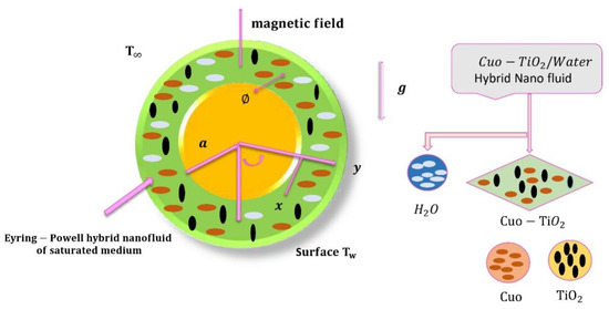
Figure 1.
Physical representation.

Table 1.
Thermo-physical characteristics of water, copper oxide () and titanium oxide () [16,34].
Table 2.
Hybrid nanofluid thermos physical properties are given below [37].
Defined stream function is . Since continuity equation is satisfied, is specified by and . We now express dimensionless quantities as follows:
We substitute Equation (7) into Equations (2) and (3). Then following dimensionless PDEs are obtained:
The dimensionless boundary conditions are transformed:
The parameters which appear in Equations (8) and (9) are magnetic parameter is define as , shows Prandl number (), Darcy parameter is presented as , where [36], thermal radiation parameter , Ecart number , Richardson number , is a heat source sink, Reynold number , Eyring-powell fluid parameter , and concentration grashof number . The coefficient of skin friction and Nusselt number are defined as follow;
where and are given as
After applying a non-similar transformation Equation (11) become
where and .
3. Local Non-Similarity Solution Method
The system of nonlinear PDEs can be solved numerically with local non-similarity method. The local non-similarity method is the most straightforward and popular approach. The truncated solution of non-similar boundary layer flow was studied by Sparrow and Quack [38]. We applied Sparrow and Quack’s methods to nonlinear PDE equations in order to obtain the local non similarity solution (8) and (9). The following scheme is applied as follows.
3.1. First Level Truncation
Since , we eliminate only the on the right side of the equation at the first level of truncation, which is the most basic type. As a result, Equations (8)–(11) become;
3.2. Second Level Truncation
All of the terms in the modified conservation equations are kept in the local non similarity approach, while the new functions are used to mask the derivatives and assuming , Therefore, calculating the derivative of Equations (8)–(10) with respect to and replace by new define functions.
3.3. Third Level Truncation
All terms are kept in both the and the equations in order to apply the local similarity method to the third level of truncation. Now, the derivatives that show up in the equations are concealed by introducing new function of , so the Equations (18)–(20) become;
4. Numerical Solutions
The author focuses to investigate non-similar solution of boundary layer flow of an Eyring-Powell hybrid nanofluid along a horizontal porous cylinder with heat source sink and viscous dissipation effects. The numerical solution is evaluated with bpv4c MATLAB built in function up to third level of truncation. An artificial neural network model which is a machine learning technique algorithm is applied to examined flow behavior. ANN and machine learning approach are most accurate approach for problem convergence.
Artificial Neural Network Design
The objective to apply ANN scheme on Eyring-Powell hybrid nano fluid past a horizontal cylinder in a non-Darcy porous medium to compute an approximate solution. In Computational Fluid Dynamics (CFD), Artificial Neural Networks (ANNs), a highly useful efficient technique for the simulation of non-Newtonian flow behavior. For each variable there is different algorithms of MLP-ANN. In MLP-ANN frameworks algorithm optimizing the data set with some mathematical functions i.e., activation function. The MLP-ANN methods’ prediction performance is based on data optimization [34]. The network model has been trained to optimize data, and its accuracy in predicting algorithms has been studied. The network model is run to get expected valuation once MLP-ANN technique has trained. Figure 2 displays, fundamental flowchart utilized in a design of MLP-ANN systems. The Feed-Forward Neural Network (FFNN) and Back-Propagation (BP) Multilayered Perceptual (MLP) network topologies are two of the most used in the proposed MLP-ANN approach because of their complex configurations. The input layer is the first layer of the MLP system; the hidden layer is the second; and the output layer is the third. A weighted neuron entered (input) the second hidden layer of this network. After passing through the input layer, the neuron signal moved on to the hidden layer, which has a variety of topologies and is the primary decision-making component (output). In MLP, each layer is interconnected. Information transmitted forward from input layer is returned to hidden layer in a feed forward network, which helps to minimize difference between stated valuations and objective valuations. This analysis, which continues while the error rate is reduced, ends when the maximum prediction efficiency is attained and MLP-ANN methods’ training is finished. There is no known, reliable model that can predict number of neurons in the hidden layer of multilayer perceptron (MLP) networks, so MLP-ANN scheme with seven neurons in hidden layer has been demonstrated, and the predictive capabilities of MLP-ANN models constructed with different numbers of neurons have been investigated. Figure 3 shows physical design of a MLP design. The MLP-ANN technique, which was used to forecast LNN, was developed using the data sets, of the data used for training, for validations, and for testing.
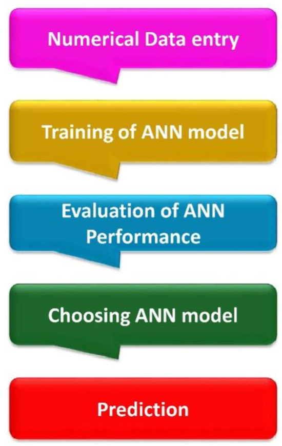
Figure 2.
The flow diagram used to create MLP-ANN schemes.
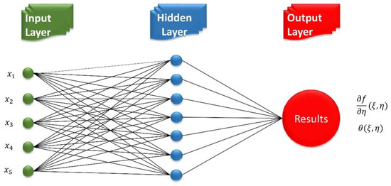
Figure 3.
A network’s MLP configuration design.
The network models’ output and hidden layers, respectively, make use of the Tan-Sig and Purelin [35] transport functions. The mathematical explanations of transport functions are as follows:
The next phase in the creation of MLP-ANN schemes is to analyze the prediction accuracy of models. The averaged relative error (ARE), mean square error (MSE), and coefficient of correlation () variables have been investigated with MLP-ANN techniques. A list of mathematical methods used to determine the efficacy factors is provided below.
5. Results and Discussion
The main goal of this study is to investigate the flow of a non-Newtonian Eyring-Powell Hybrid Nanofluid (EPHNF) model past a horizontal cylinder immersed in a porous medium with viscous dissipation and heat source sink effects. The Tiwari-Das model is used to develop flow problem for hybrid nanoparticles over a horizontal cylinder [35]. The Local Non-Similarity solution technique is used to numerically solve boundary layer flow of a Eyring-Powell Hybrid Nanofluid (EPHNF) across a cylinder up to a third level of truncation Equations (21)–(27). In local non-Similarity solution technique, all values on the right side of the equation that take the form of will be eliminated at first level of truncation. In second truncation level, we define a new function and replace the old function in the form of by these new functions. Similarly, for third level of truncation, a new function was defined and the equation was solved.
The pertinent parameters (i.e., , , , , and ) of interest are shown in Table 3. Table 4 displays the gradient, Mu, and MSE tabulated values for boundary layer flow of non-Newtonian hybrid nanofluid for scenario 1 of cases 1 to 3. In Table 4, performance is [ and ] is attain against iterations [517, 68, and 37], however is noted to be and 1.00. ANN defines an error or cost function that quantifies the difference between actual and predicted results with MLP-ANN. One simple method for measuring error is to use Mean Squared Error (MSE). The training outcomes of the suggested ANN techniques are displayed in Figure 4a for scenario 1 of cases 1–3. It is clear that MSE valuations, which were high in the early training parts, decline as the number of epochs diminishes. MSE values are decreased at each epoch in accordance with the function of MLP model, and ANN schemes’ training session concludes when the smallest MSE values are acquired since maximum accuracy has been attained. These low MSE values show that the developed ANN algorithms’ training phase effectively employed very minimal error levels. Figure 4b displays the training setting for ANN methods. Network parameter optimization is made possible via gradient descent, which moves in the opposite direction of the gradient of the loss function. As epoch values fall, the gradient increases, as shown in Figure 4b. Consequently, the verification tests have no value. Error histogram displays the error between actual and predicted values during ANN training. These error show how the actual and predicted outcomes differ.
Table 3.
Valuations of input parameters used in ANN models.
Table 4.
Analogous analysis across backpropagation networks for scenario 1 of case 1–3.
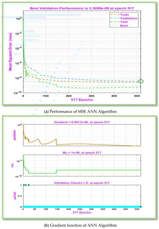
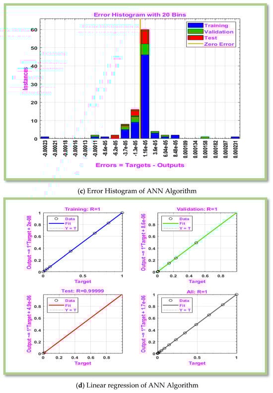
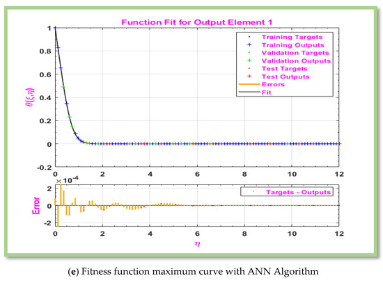
Figure 4.
Graphical representation of MLP-ANN algorithm for effectiveness and convergence of results displays for scenario 1.
Figure 4c displays the error histogram between estimated and actual values of numerical data of the proposed non-Newtonian Eyring-Powell hybrid nanofluid past a horizontal cylinder. It is detected that the error plots reveal that error rates attained for each data point close to zero error-line. The current state of the data used for testing, training, and validating ANN schemes is shown in Figure 4d. Function curve is plotted in Figure 4d to show that the output satisfy the boundary condition. The plots show the target data on -axis and outputs of ANN schemes on-axis. The proximity of the data points to the zero-error line indicates that error between target data and ANN’s predicted value is low, while the fitted line is close to zero line, indicating that the average error is also significantly reduced. values that are nearly equal to one are strongly associated with improving accuracy of ANN algorithm. Furthermore, it should be noted that each step’s calculated values are nearly equal to 1. Figure 4d makes it clear that ANN algorithm is developed in order to produce a predicted value. In ANN, a function fit plot is basically a visual representation of how the model’s outputs match actual outputs during the training or testing phase. Figure 4e provides a visual evaluation of ANN model’s performance. The ANN model vanished at about error-line, according to graphs, and expected and actual outputs of model roughly match.
Table 5 displays the gradient, Mu, and MSE tabulated values for scenarios 2 case 1–3. The numerical value of gradient as Mu as and MLP-ANN performance as , and against the epochs 10,11, and 10. Figure 5a provides a visual representation of MSE for scenario 2. Figure 5a demonstrated the convergence of the proposed MLP-ANN model, and it is shown that the accuracy was reached at . Figure 5b displayed the gradient’s graphical representation for scenario 2. Figure 5b shows that the convergence rata is while moving in opposite direction as the gradient of the loss function. The error histogram between predicted and actual values of the proposed fluid model beyond a horizontal cylinder is displayed in Figure 5c. The linear regression and correlation index for scenario 2 are shown in Figure 5d. When the correlation index value is close to 1, the best-fitting model is shown. According to Figure 5d, . Figure 5e displays the ideal curve fitness function for scenario 2.
Table 5.
Analogous analysis across backpropagation networks for scenario 2 of case 1–3.
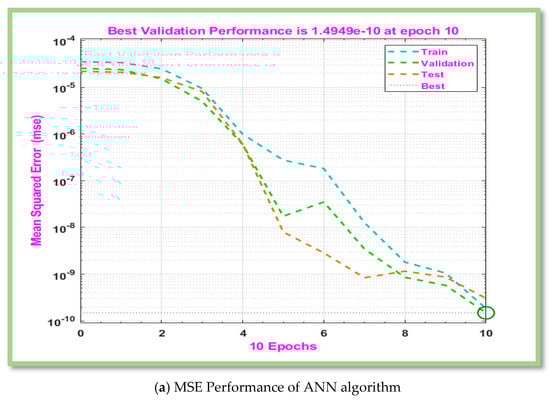
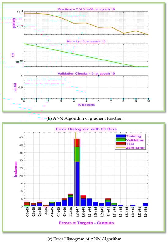
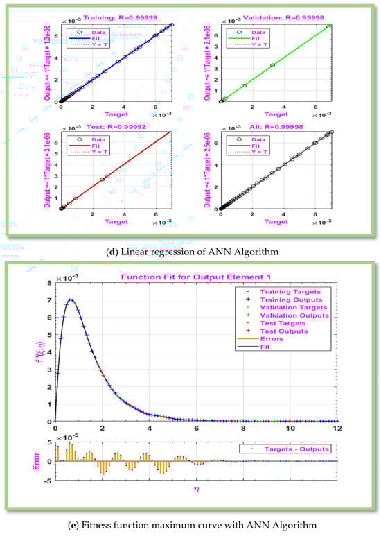
Figure 5.
Graphical representation of MLP-ANN algorithm for effectiveness and convergence of results displays for scenario 2.
Table 6, Table 7, Table 8 and Table 9 displays computed results for the gradient, Mu, and MSE for cases 1–3 of scenarios 3–6. The MLP-ANN most effective Gradient value for case 1 of scenario 3–6 is at [], ], [] and [] against epoch [10, 10, 9], [48, 19, 15], [119, 217, 19], and [145, 146, 25] respectively. The calculated values of Mu and performance for case 1–3 of scenarios 3–6 are [ and and ,], respectively. In Figure 6a, Figure 7a, Figure 8a and Figure 9a, MSE for scenarios 3–6 is displayed graphically. According to Figure 6a, Figure 7a, Figure 8a and Figure 9a, precision of proposed ANN model is ,and respectively. For scenarios 3–6, Figure 6b, Figure 7b, Figure 8b and Figure 9b displayed the gradient curve convergence of non-Newtonian hybrid nanofluid solution past a horizontal circular cylinder. The error histogram for situations 3–6 is displayed in Figure 6c, Figure 7c, Figure 8c and Figure 9c. The linear regression and correlation index for scenarios 3–6 are shown in Figure 6d, Figure 7d, Figure 8d and Figure 9d. For scenario 3–6 of Figure 6e, Figure 7e, Figure 8e and Figure 9e show the curve fitness function.
Table 6.
Analogous analysis across backpropagation networks for scenario 3 of case 1–3.
Table 7.
Analogous analysis across backpropagation networks for scenario 4 of case 1–3.
Table 8.
Analogous analysis across backpropagation networks for scenario 5 of case 1–3.
Table 9.
Analogous analysis across backpropagation networks for scenario 6 of case 1–3.
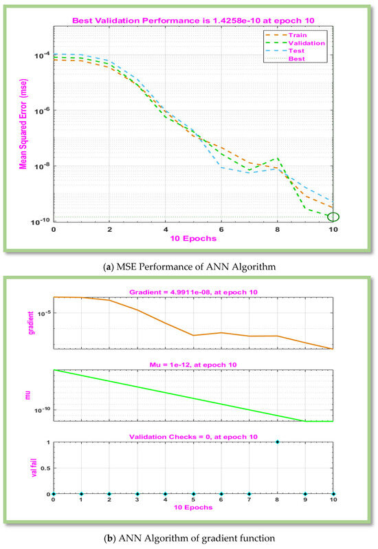
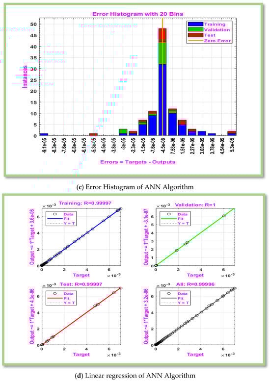
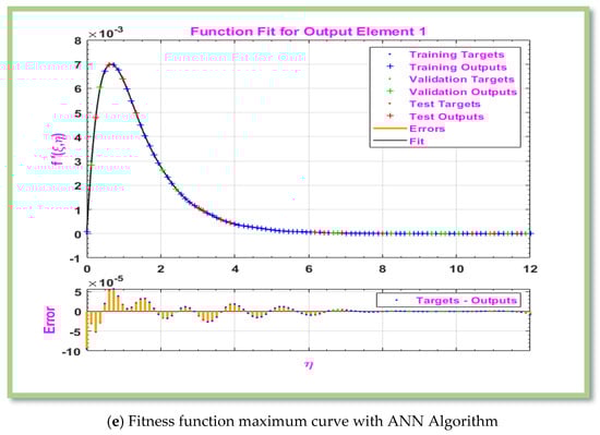
Figure 6.
Graphical representation of MLP-ANN algorithm for effectiveness and convergence of results displays for scenario 3.
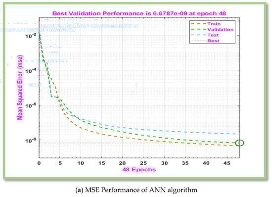
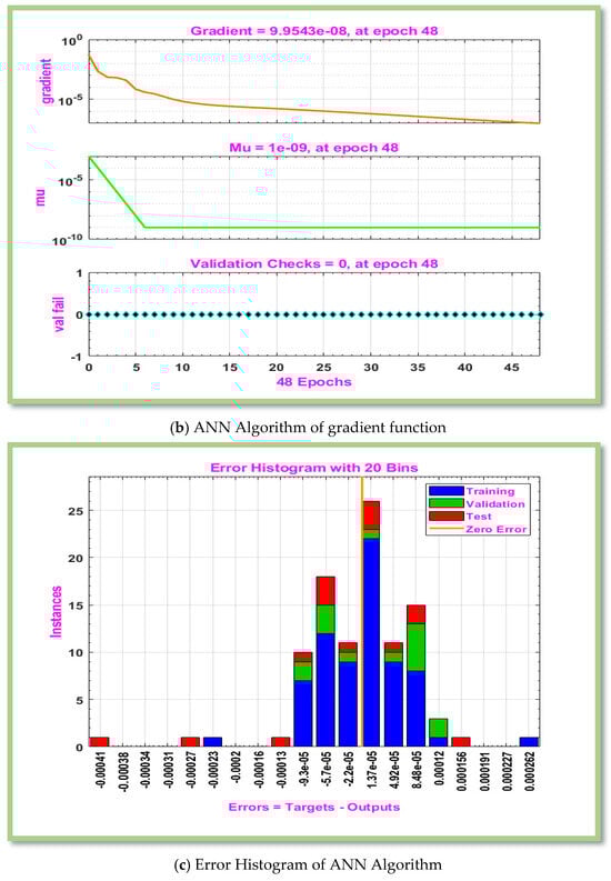
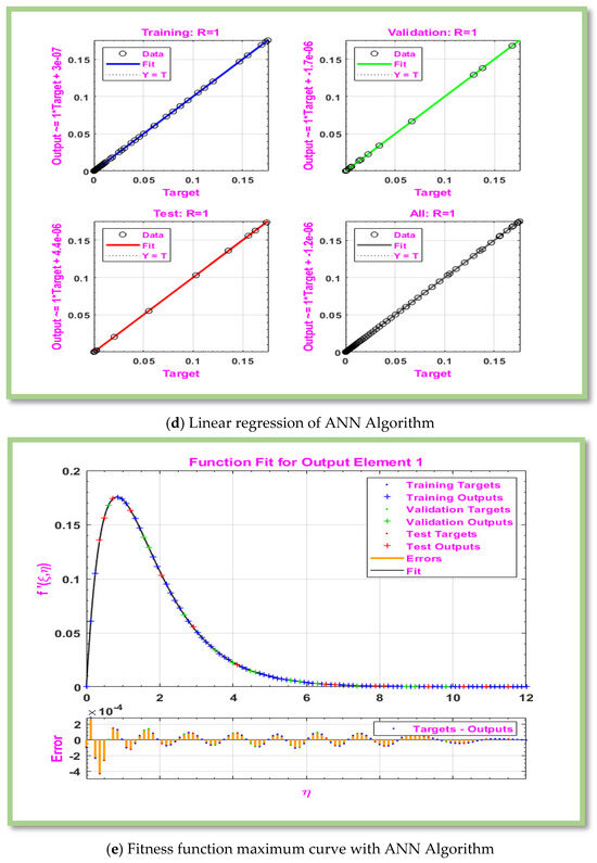
Figure 7.
Graphical representation of MLP-ANN algorithm for effectiveness and convergence of results displays for scenario 4.
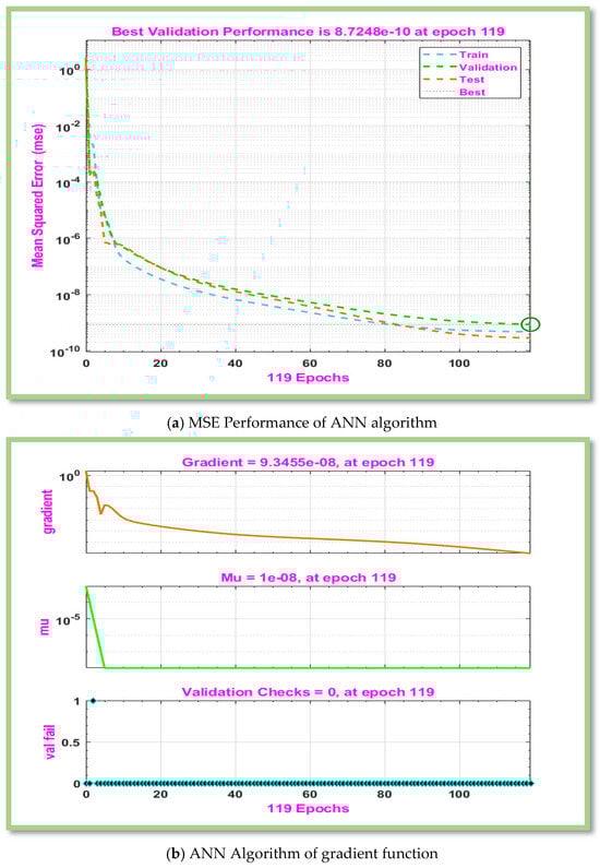
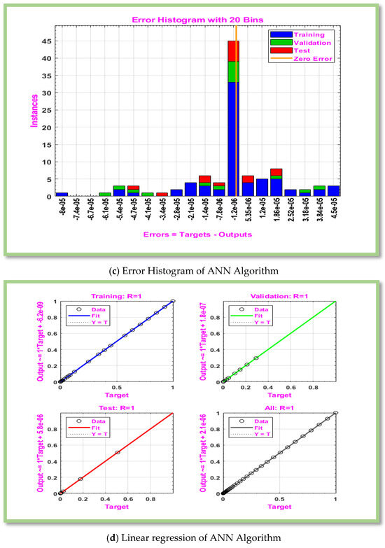
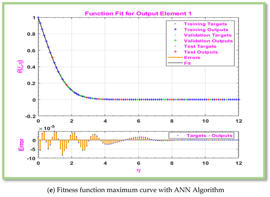
Figure 8.
Graphical representation of MLP-ANN algorithm for effectiveness and convergence of results displays for scenario 5.
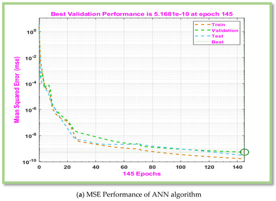
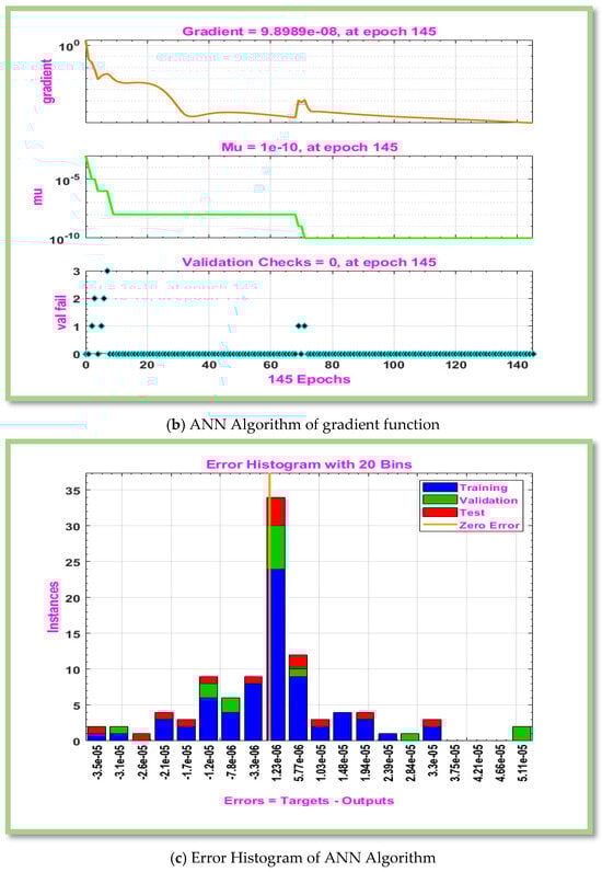
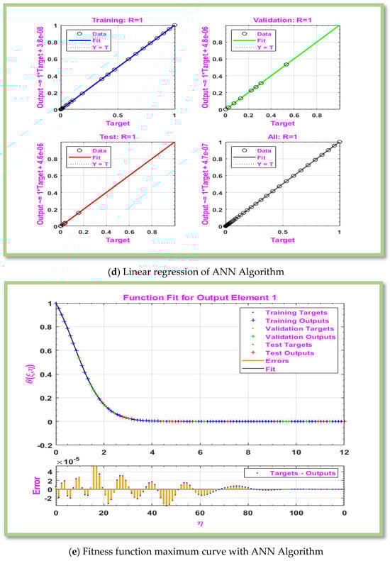
Figure 9.
Graphical representation of MLP-ANN algorithm for effectiveness and convergence of results displays for scenario 6.
The matrices pertaining to values and patterns in the residual are displayed in Table 10. For scenarios 1–6, these matrices have realistic characteristics that are similar to Sum of Square Error (SSE), R-square (), Adj R-sq, and MSE. The following factors are observed when looking for matrices. The R-square and Adj R-sq values are close to one, as can be shown in Table 10, suggesting a strong relationship between actual and expected values in scenarios. Furthermore, the model’s suitability is demonstrated by high numerical values of R-square and Adj R-square, which are close to zero. However, the model correctness is addressed via RMSE. The Root Means Squared Error (RMSE) number is low, as Table 10 demonstrates. The fact that RMSE and SSE differ depending on the situation suggests that the model’s prediction might not be accurate for different data sets.
Table 10.
For scenarios 1–6, residual fit for Eyring-Powell fluid model derivatives.
The residual graph can be used to assess how well a model matches the data. The residual should preferably be randomly distributed around zero to demonstrate that there isn’t a systematic error. For scenarios 1–6, Figure 10a–e displays the residual analysis of MHD boundary layer flow of a non-Newtonian Eyring-Powell hybrid nanofluid across a horizontal porous cylinder.
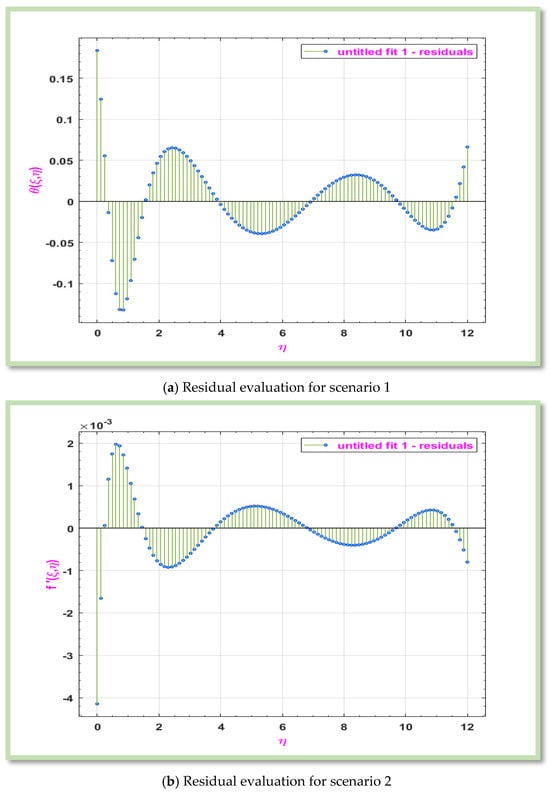
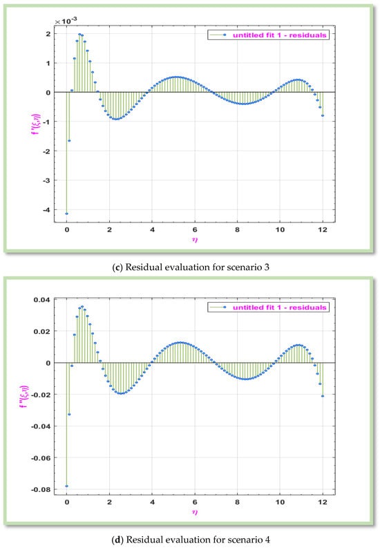
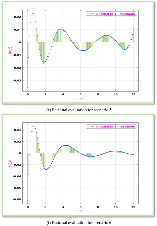
Figure 10.
Graphical representation of Residual for considered problem for different scenarios.
Figure 11 illustrates how the radiation parameter affects MHD boundary layer flow of a hybrid nanofluid past a horizontal porous cylinder. The is crucial when examining fluid velocity and heat transfer in MHD boundary layer flow of non-Newtonian hybrid nanofluids. Fluid velocity increases as values rise, as shown in Figure 11.
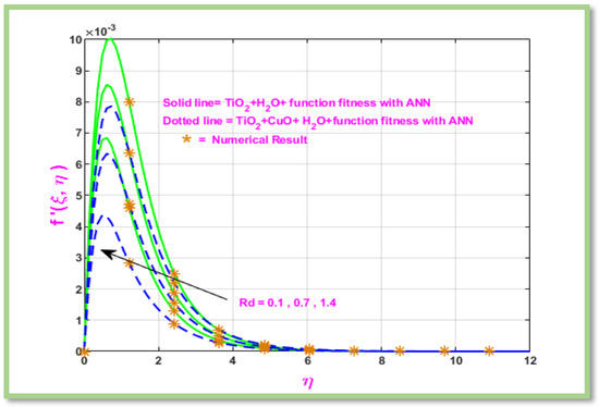
Figure 11.
Velocity profile of .
Figure 12 shows the impact of on boundary layer flow of hybrid nanofluid flows past a porous cylinder. Figure 12 illustrates velocity will decrease when Eyring-Powell fluid parameter () increases.
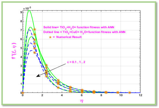
Figure 12.
Velocity profile of .
Figure 13 Show the velocity of boundary layer flow of a hybrid nanofluid along a horizontal porous cylinder dramatically drops as δ increases. This property is particularly helpful in applications like electromagnetic flow control, where stabilizing fluid motion or reducing flow velocity are the main objectives.
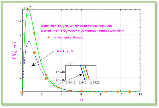
Figure 13.
Velocity profile of , where single nano particle we show solid line and green color and for hybrid particle we have a dotted line with blue color.
It is noted that when there is MHD in flow, the Lorentz force increases which opposes the flow. This phenomenon is highlighted in Figure 14 which shows when the value of increases then velocity of fluid decline across a horizontal porous cylinder. It illustrates the graphical conclusion for velocity with the influence of magnetic parameter; the equation’s velocity decreases when is increase.
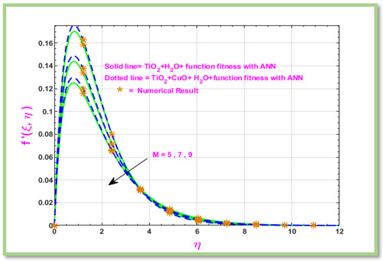
Figure 14.
Velocity profile of M.
Figure 15 show the influence of a parameter on the flow of a boundary layer Eyring-Powell hybrid nanofluid across a horizontal porous cylinder. It illustrates the graphical conclusion for velocity with the influence of the heat source/sink, the equation’s velocity increases when is increase.
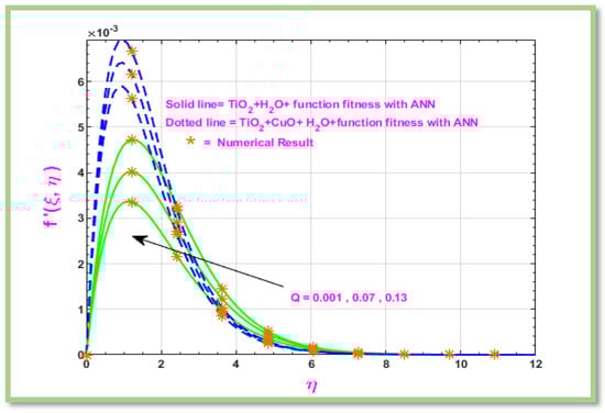
Figure 15.
Velocity profile of Q.
In Figure 16, using water as basis fluid, hybrid nanoparticles, such as , and , are present. Figure 16 discusses the effects of Richardson’s number () on velocity. The velocity close to the surface decreases as effects of increases.
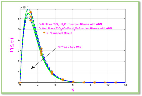
Figure 16.
Velocity profile of Ri.
Figure 17 demonstrates the impact of the radiation parameter () on hybrid nanofluids that are non-Newtonian. The relative significance of radiative heat transfer in relation to conductive heat transfer is indicated by the radiation parameter. It is essential in situations where thermal radiation cannot be disregarded and in high-temperature systems. The behavior of heat transfer systems under varied thermal and fluid flow conditions can be better understood and predicted by scientists and engineers through analysis. It has been noted that when Rd increases, the fluid’s temperature rises.
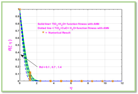
Figure 17.
Graphical representation of temperature with respect to .
Figure 18 Show the impact of the Eyring-Powell parameter on fluid temperature. The molecular relaxation and flow resistance under stress are represented, respectively, by the Eyring-Powell parameters. Since these parameters provide details on the fluid’s non-Newtonian characteristics and stress tolerance, the model can be used to a wide range of scientific and technical problems. Viscosity dissipation is applied to an Eyring-powell fluid in the boundary layer outside of a horizontal cylinder. Figure 18 shows that the temperature of the fluid increases as the value of ε increases.
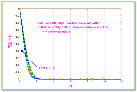
Figure 18.
Graphical representation of temperature with respect to .
Figure 19 Show the effect of the Concentration Grashof number on fluid temperature. Concentration Grashof number accounts for the importance of buoyancy-induced flow due to concentration gradients. It finds important uses in the study of flows that are mostly caused by solute convection, specifically in the field of environmental processes and natural convection systems, as well as in certain industrial applications. As seen in Figure 19, that the temperature of the fluid is overlapping when increases the value of .
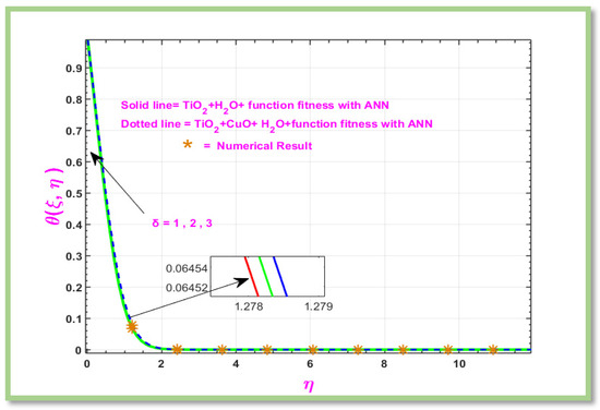
Figure 19.
Graphical representation of temperature with respect to , where single nano particle we show solid line and green color and for hybrid particle we have a dotted line with blue color.
Figure 20 discussed the magnetic parameter effect on the boundary layer flow of hybrid Nano fluid past a horizontal porous cylinder. represents how strongly the magnetic field affects the fluid flow. The parameter value is large if magnetic forces dominate inertial forces. Calculating has immense importance in designing and analyzing systems of conducting fluids under the influence of a magnetic field. As seen in Figure 20, Temperature is increase when increase the value of M.
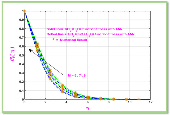
Figure 20.
Graphical representation of temperature with respect to .
Figure 21 discussed the heat source/sink () effect on the boundary layer flow of hybrid Nano fluid past a horizontal porous cylinder in a heat transfer problem, the heat source/sink term has a major impact on the flow behavior, energy balance, and temperature distribution. As seen in Figure 21, Temperature increases when increase.
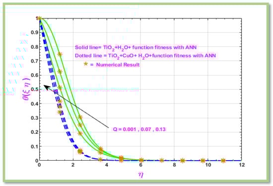
Figure 21.
Graphical representation of temperature with respect to Q.
Figure 22 discusses the impact of Richardson’s parameter () on boundary layer flow of hybrid Nano fluid past a horizontal porous cylinder temperature. Richardson’s parameter helps characterize the kind and behavior of convection within a system by indicating whether the flow is dominated by buoyancy forces (natural convection) or shear forces (forced convection).
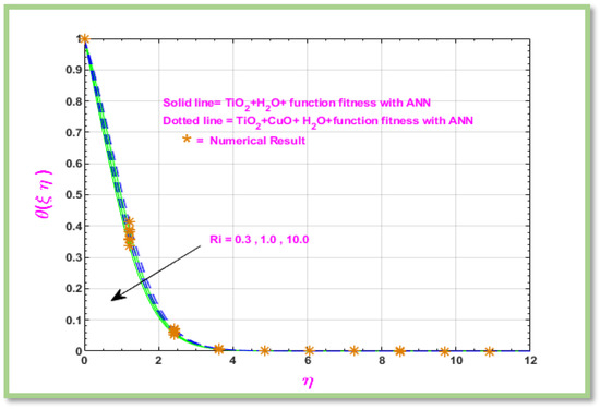
Figure 22.
Graphical representation of temperature with respect to
.
As seen in Figure 22, Additionally, it is noted that the temperature profile asymptotically meets the boundary requirement. The rate of temperature decreases when increases the value of . Also, in Table A1 Comparison of for different values of Pr with previous works [30,31,32,33,34,35,36,37,38,39,40,41] and it is clear that, the present values are same obtained in [41].
6. Conclusions
- Examining the boundary layer flow and heat transfer enhancement by the use of an Eyring-Powell hybrid nanofluid past a horizontal non-Darcy porous medium cylinder with a heat source sink and viscous dissipation effect is the main objective of our research. Governing flow equations are developed using Tiwari Das model for the investigation of hybrid nanoparticles. The non-similar transformation is applied to obtain the dimensionless PDEs. The key findings from the results that were shown are as follows:
- Velocity profile versus dimensionless parameter increases with increasing Rd and Q parameters. The velocity profile decreases as the values of parameters ε, M, and Ri increase, and the values of parameter δ overlap.
- As the and parameters rise, the temperature profile rises as well. The temperature profile drops as parameters rise, and the values of the parameter overlap.
- A negligible error margin is observed when comparing the output predicted by the supervised machine learning method ANN with the computed results.
- Because of its excellent accuracy, which held up through training, testing, and validation, the proposed ANN model was regarded as reliable when compared to the computational approaches.
Author Contributions
Conceptualization, M.A.Y. and S.S.A.; Funding acquisition, M.A.L.; Investigation, M.I.K. and S.S.A.; Project administration, A.Z.; Software, P.O.M.; Supervision, P.O.M.; Validation, A.Z.; Writing—original draft, M.A.Y. and M.I.K.; Writing—review & editing, M.A.L. All authors have read and agreed to the published version of the manuscript.
Funding
This research received no external funding.
Data Availability Statement
Data are contained within the article.
Acknowledgments
This work was supported by the Deanship of Scientific Research, Vice Presidency for Graduate Studies and Scientific Research, King Faisal University, Saudi Arabia (Project No. KFU251204).
Conflicts of Interest
The authors declare no conflict of interest.
Nomenclature
| Grashof number | dimensionless stream function |
| gravitational acceleration | skin friction coefficient |
| magnetic parameter | thermal conductivity |
| Darcy parameter | specific heat |
| local Nusselt number | free stream temperature |
| Prandtl number | uniform transpiration |
| radiation parameter | stream function |
| temperature | coefficient of thermal expansion |
| dimensionless coordinate in the radial | thermal diffusivity |
| dimensionless coordinate in the tangential | electric conductivity |
| velocity component in x, y directions | dimensionless temperature |
| horizontal circular cylinder’s radius | dynamic viscosity |
| radiative heat flux | kinematic viscosity |
| surface conditions | non-Newtonian Eyring parameter |
| Cartesian coordinates | ternary Nano fluid density |
| magnetic field | Eyring-powell parameter |
| inertial drag coefficient | Material Constant |
| Forchheimer parameter | Subscripts |
| Concentration grashof number | Nano fluid |
| PDEs Partial differential equations | hybrid Nano fluid |
| Heat source coefficient | |
| K permeability coefficient |
Appendix A
Table A1.
Comparison of for different values of Pr [39,40,41].
Table A1.
Comparison of for different values of Pr [39,40,41].
| [39] | [40] | [41] | ||
|---|---|---|---|---|
| 0.8 1.0 1.2 1.4 | 1.0000 | 1.00002 | 0.866575 1.000000 1.120662 1.231583 | 0.866575 1.000000 1.120662 1.231583 |
References
- Jaber, K.K. Influence of Dofour and Soret on Eyrig-Powell Nanofluid Flow from A Circular Cylinder with Viscous Dissipation. Eur. J. Math. Stat. 2023, 4, 69–77. [Google Scholar] [CrossRef]
- Kumaran, G.; Sivaraj, R.; Prasad, V.R.; Beg, O.A.; Sharma, R.P. Finite difference computation of free magneto-convective Powell-Eyring nanofluid flow over a permeable cylinder with variable thermal conductivity. Phys. Scr. 2020, 96, 025222. [Google Scholar] [CrossRef]
- Afaq, H.; Azhar, E.; Kamran, A. Modeling and analysis of heat transfer in Eyring–Powell fluids with magnetic and viscous dissipation: Applications to MHD systems. Multiscale and Multidisciplinary Modeling. Exp. Des. 2025, 8, 168. [Google Scholar]
- Ali, N.; Nazeer, F.; Nazeer, M. Flow and heat transfer analysis of an Eyring–Powell fluid in a pipe. Z. Naturforsch. A 2018, 73, 265–274. [Google Scholar] [CrossRef]
- Yang, M.; Abbas, M.A.; Khudair, W.S. Energy and temperature-dependent viscosity analysis on magnetized Eyring-Powell fluid oscillatory flow in a porous channel. Energies 2021, 14, 7829. [Google Scholar] [CrossRef]
- Firdous, H.; Saeed, S.T.; Ahmad, H.; Askar, S. Using non-Fourier’s heat flux and non-Fick’s mass flux theory in the radiative and chemically reactive flow of Powell–Eyring fluid. Energies 2021, 14, 6882. [Google Scholar] [CrossRef]
- Gaffar, S.A.; Prasad, V.R.; Reddy, E.K. Magnetohydrodynamic free convection flow and heat transfer of non-Newtonian tangent hyperbolic fluid from horizontal circular cylinder with Biot number effects. Int. J. Appl. Comput. Math. 2017, 3, 721–743. [Google Scholar] [CrossRef]
- Turabi, Y.U.U.B.; Munir, S.; Amin, A. Numerical analysis of convective transport mechanisms in two-layer ternary (TiO2−SiO2−Al2O3) Casson hybrid nanofluid flow in a vertical channel with heat generation effects. Numer. Heat Transf. Part A Appl. 2023, 1–15. [Google Scholar] [CrossRef]
- Amin, A.; Munir, S.; Farooq, U. Flow dynamics and convective transport analysis of two-layered dissipative Casson hybrid nanofluid flow in a vertical channel. Proc. Inst. Mech. Eng. Part C J. Mech. Eng. Sci. 2024, 238, 395–404. [Google Scholar] [CrossRef]
- Das, S.; Mahato, N.; Ali, A.; Jana, R.N. Dynamical behaviour of magneto-copper-titania/water-ethylene glycol stream inside a gyrating channel. Chem. Phys. Lett. 2022, 793, 139476. [Google Scholar] [CrossRef]
- Ali, A.; Das, S.; Jana, R.N. MHD gyrating stream of non-Newtonian modified hybrid nanofluid past a vertical plate with ramped motion, Newtonian heating and Hall currents. ZAMM-J. Appl. Math. Mech. Z. Für Angew. Math. Und Mech. 2023, 103, e202200080. [Google Scholar]
- Das, S.; Mahato, N.; Ali, A.; Jana, R.N. Aspects of Arrhenius kinetics and Hall currents on gyratory Couette flow of magnetized ethylene glycol containing bi-hybridized nanomaterials. Heat Transf. 2023, 52, 2995–3026. [Google Scholar] [CrossRef]
- Choi, S.U.; Eastman, J.A. Enhancing Thermal Conductivity of Fluids with Nanoparticles; (No. ANL/MSD/CP-84938; CONF-951135-29); Argonne National Lab. (ANL): Argonne, IL, USA, 1995. [Google Scholar]
- Jan, A.; Mushtaq, M.; Khan, M.I.; Farooq, U. Integrated artificial intelligence and non-similar analysis for forced convection of radially magnetized ternary hybrid nanofluid of Carreau-Yasuda fluid model over a curved stretching surface. Int. J. Numer. Methods Fluids 2024, 96, 1864–1882. [Google Scholar]
- Usman, M.; Areshi, M.; Khan, N.; Eldin, M.S. Revolutionizing heat transfer: Exploring ternary hybrid nanofluid slip flow on an inclined rotating disk with thermal radiation and viscous dissipation effects. J. Therm. Anal. Calorim. 2023, 148, 9131–9144. [Google Scholar] [CrossRef]
- Zeeshan, A.; Khan, M.I.; Majeed, A.; Alhodaly, M.S. Temporal stability analysis and thermal performance of non-Newtonian nanofluid over a shrinking wedge. Propuls. Power Res. 2024, 13, 586–596. [Google Scholar]
- Shoaib, M.; Javed, T. Sensitivity analysis of non-isothermal mixed convective heat and mass transfer in nanofluid flow over a horizontal circular cylinder with Brownian motion. Numer. Heat Transf. Part B Fundam. 2024, 85, 984–1008. [Google Scholar]
- Saeed, A.; Alsubie, A.; Kumam, P.; Nasir, S.; Gul, T.; Kumam, W. Blood based hybrid nanofluid flow together with electromagnetic field and couple stresses. Sci. Rep. 2021, 11, 12865. [Google Scholar]
- Shoaib, M.; Javed, T. MHD radiative natural convective heat transfer enhancement for Casson nanofluid flow on a horizontal circular cylinder. J. Comput. Sci. 2024, 78, 102257. [Google Scholar]
- Amin, A.; Munir, S.; Farooq, U. Investigating flow features and heat/mass transfer in two-layer vertical channel with Gr-TiO2 hybrid nanofluid under MHD and radiation effects. J. Magn. Magn. Mater. 2023, 578, 170800. [Google Scholar]
- Qayyum, M.; Afzal, S.; Saeed, S.T.; Akgül, A.; Riaz, M.B. Unsteady hybrid nanofluid (Cu-UO2/blood) with chemical reaction and non-linear thermal radiation through convective boundaries: An application to bio-medicine. Heliyon 2023, 9, e16578. [Google Scholar]
- Amin, A.; Munir, S.; Farooq, U. Comparative study of MHD boundary layer flow of hybrid nanofluid in a channel. ZAMM-J. Appl. Math. Mech. Z. Für Angew. Math. Und Mech. 2024, 104, e202300050. [Google Scholar]
- Ali, A.; Mebarek-Oudina, F.; Barman, A.; Das, S.; Ismail, A.I. Peristaltic transportation of hybrid nano-blood through a ciliated micro-vessel subject to heat source and Lorentz force. J. Therm. Anal. Calorim. 2023, 148, 7059–7083. [Google Scholar]
- Khan, M.I.; Zeeshan, A.; Ellahi, R.; Bhatti, M.M. Advanced Computational Framework to Analyze the Stability of Non-Newtonian Fluid Flow through a Wedge with Non-Linear Thermal Radiation and Chemical Reactions. Mathematics 2024, 12, 1420. [Google Scholar] [CrossRef]
- Prasad, V.R.; Abdul Gaffar, S.; Keshava Reddy, E.; Bég, O.A. Numerical study of non-Newtonian Jeffreys fluid from a permeable horizontal isothermal cylinder in non-Darcy porous medium. J. Braz. Soc. Mech. Sci. Eng. 2015, 37, 1765–1783. [Google Scholar]
- Jan, A.; Mushtaq, M.; Hussain, M. Heat transfer enhancement of forced convection magnetized cross model ternary hybrid nanofluid flow over a stretching cylinder: Non-similar analysis. Int. J. Heat Fluid Flow 2024, 106, 109302. [Google Scholar]
- Khan, U.; Zaib, A.; Ishak, A. Non-similarity solutions of radiative stagnation point flow of a hybrid nanofluid through a yawed cylinder with mixed convection. Alex. Eng. J. 2021, 60, 5297–5309. [Google Scholar] [CrossRef]
- Prasad, V.R.; Vasu, B.; Be’g, O.A. Thermo-diffusion and diffusion-thermo effects on free convection flow past a horizontal circular cylinder in a non-Darcy porous medium. J. Por. Media. 2013, 16, 315–334. [Google Scholar] [CrossRef]
- Subhashini, S.V.; Samuel, N. Non-Similar Solution of a Steady Compressible Boundary Layer Flow over a Thin Cylinder. Front. Heat Mass Transf. FHMT 2016, 7, 29. [Google Scholar]
- Lawal, M.O.; Tijani, Y.O.; Ajadi, S.O.; Kasali, K.B. Simulation of the laminar thermal boundary layer problem over a flat plate by exploring the local non-similarity technique. Int. J. Model. Simul. 2023, 1–12. [Google Scholar] [CrossRef]
- Chu, Y.M.; Khan, M.I.; Abbas, T.; Sidi, M.O.; Alharbi, K.A.M.; Alqsair, U.F.; Khan, S.U.; Khan, M.R.; Malik, M.Y. Radiative thermal analysis for four types of hybrid nanoparticles subject to non-uniform heat source: Keller box numerical approach. Case Stud. Therm. Eng. 2022, 40, 102474. [Google Scholar]
- Zeeshan, A.; Khalid, N.; Ellahi, R.; Khan, M.I.; Alamri, S.Z. Analysis of nonlinear complex heat transfer MHD flow of Jeffrey nanofluid over an exponentially stretching sheet via three phase artificial intelligence and Machine Learning techniques. Chaos Solitons Fractals 2024, 189, 115600. [Google Scholar] [CrossRef]
- Mohamed MK, A.; Sarif, N.M.; Kasim AR, M.; Noar NA, Z.M.; Salleh, M.Z.; Ishak, A. Effects of viscous dissipation on free convection boundary layer flow towards a horizontal circular cylinder. ARPN J. Eng. Appl. Sci. 2016, 11, 7258–7263. [Google Scholar]
- Yadav, N.; Yadav, A.; Kumar, M. An Introduction to Neural Network Methods for Differential Equations; Springer: Berlin, Germany, 2015; Volume 1, p. 7. [Google Scholar]
- Vasu, B.; Prasad, V.R.; Bég, O.A. Thermo-diffusion and diffusion-thermo effects on MHD free convective heat and mass transfer from a sphere embedded in a non-Darcian porous medium. J. Thermodyn. 2012, 2012, 725142. [Google Scholar] [CrossRef]
- Ramachandra Prasad, V.; Subba Rao, A.; Anwar Bég, O. Flow and heat transfer of Casson fluid from a horizontal circular cylinder with partial slip in non-Darcy porous medium. J. Appl. Computat. Math. 2013, 2, 2. [Google Scholar]
- Kaneez, H.; Baqar, A.; Andleeb, I.; Hafeez, M.B.; Krawczuk, M.; Jamshed, W.; Eid, M.R.; Abd-Elmonem, A. Thermal analysis of magnetohydrodynamics (MHD) Casson fluid with suspended iron (II, III) oxide-aluminum oxide-titanium dioxide ternary-hybrid nanostructures. J. Magn. Magn. Mater. 2023, 586, 171223. [Google Scholar] [CrossRef]
- Minkowycz, W.J.; Sparrow, E.M.; Schneider, G.E.; Pletcher, R.H. Handbook of Numerical Heat Transfer; Wiley Interscience: New York, NY, USA, 1988. [Google Scholar]
- Grubka, L.J.; Bobba, K.M. Heat transfer characteristics of a continuous stretching surface with variable temperature. J. Heat Transf. 1985, 107, 248–250. [Google Scholar] [CrossRef]
- Vajravelu, K.; Prasad, K.V.; Santhi, S.R. Axisymmetric magneto-hydrodynamic (MHD) flow and heat transfer at a non-isothermal stretching cylinder. Appl. Math. Comput. 2012, 219, 3993–4005. [Google Scholar] [CrossRef]
- Reddy SR, R.; Bala Anki Reddy, P.; Rashad, A.M. Activation energy impact on chemically reacting Eyring–Powell nanofluid flow over a stretching cylinder. Arab. J. Sci. Eng. 2020, 45, 5227–5242. [Google Scholar] [CrossRef]
Disclaimer/Publisher’s Note: The statements, opinions and data contained in all publications are solely those of the individual author(s) and contributor(s) and not of MDPI and/or the editor(s). MDPI and/or the editor(s) disclaim responsibility for any injury to people or property resulting from any ideas, methods, instructions or products referred to in the content. |
© 2025 by the authors. Licensee MDPI, Basel, Switzerland. This article is an open access article distributed under the terms and conditions of the Creative Commons Attribution (CC BY) license (https://creativecommons.org/licenses/by/4.0/).