Enhancing Frequency Event Detection in Power Systems Using Two Optimization Methods with Variable Weighted Metrics

Abstract

This research presents a novel technique that refines the performance of a frequency event detection algorithm with four adjustable parameters based on signal processing and statistical methods. The algorithm parameters were optimized using two well-established optimization techniques: Grey Wolf Optimization and Particle Swarm Optimization. Unlike conventional approaches that apply equally weighted metrics within the objective function, this work implements variable weighted metrics that prioritize specificity, thereby strengthening detection accuracy by minimizing false-positive events. Realistic small- and large-scale frequency datasets were processed and analyzed, incorporating various events, quasi-events, and non-events obtained from a phasor measurement unit in the Western Interconnection. An analytical comparison with an algorithm that uses equally weighted metrics was performed to assess the proposed method’s effectiveness. The results demonstrate that the application of variable weighted metrics enables the detection algorithm to identify frequency non-events, thereby significantly reducing false positives reliably.

1. Introduction

Integrating renewable energy source (RES) into power systems offers environmental and economic benefits but challenges frequency stability. The reduced inertia from replacing traditional generators increases rate of change of frequency (ROCOF), potentially triggering load-shedding controllers for minor imbalances and weakening frequency control mechanisms [1].

Maintaining power system frequency within permissible limits around a nominal value is crucial for reliable operations. Severe frequency deviations, known as frequency events, indicate imbalances between generation and demand. In such events, balancing authorities must provide frequency response services to maintain system reliability [2].

Severe frequency events and inadequate responses can cause system collapse and service disruptions. Accurate event detection through well-designed algorithms enhances grid stability and reliability. Optimization techniques significantly improve detection performance, reducing system failure risk and ensuring reliable power supply [3].

Frequency event detection in power systems is a critical task for ensuring grid stability and reliability. While modern machine and deep learning methods have demonstrated great promise in various domains, they face significant challenges when applied to frequency event detection, primarily due to data availability. These methods typically require large, diverse datasets of frequency event samples for training and validation, which are often unavailable in the context of power systems, as frequency events occur rarely—typically two to three times per month.

Existing detection methods using conventional optimization techniques, such as metastatic methods, assign equal weight and importance to detection metrics like accuracy, sensitivity, precision, and specificity within the objective function. However, these methods may suffer from high false positive rates or insufficient detection accuracy, particularly when data are sparse.

To address these issues, this study employs metastatic methods, specifically Grey Wolf Optimization (GWO) and Particle Swarm Optimization (PSO), to enhance the detection performance of a Wavelet Transform-Based Algorithm (WTBA). The novelty of the proposed approach lies in incorporating variable weighted metrics that prioritize specificity, correctly identifying frequency non-event incidents, reducing false positives, and improving the accuracy of event detection. Further elaboration and details about the frequency event detection and optimization methods will be provided in the following sections.

1.1. Background

This work builds on existing research to enhance frequency event detection. Previous work introduced the WTBA with four tunable parameters based on estimated values [4], compared it with an alternative algorithm [5], and examined the impact of signal processing techniques.

While earlier studies used equally weighted metrics in the objective function for optimization, this study employs variably weighted metrics to optimize algorithm parameters. For validation, the WTBA performance with estimated and optimized parameters was compared with equal weights. Optimization results for equal and variable weights were analyzed, and the proposed method was evaluated against another algorithm [6], demonstrating its effectiveness.

1.2. Event Detection Methods in Power Systems

Frequency event detection techniques are classified based on their methodologies into four main categories: signal-processing-based, statistical-based, machine-learning-based, and hybrid methods. The latter combines different techniques from other methods. This subsection briefly reviews the abovementioned techniques used to design frequency event detection algorithms.

1.2.1. Signal Processing Method

Anshuman et al. [7] used Discrete Wavelet Transform (DWT) to discern transient and oscillatory events, proposing an energy indicator derived from voltage and frequency signals. Kim et al. [8] introduced a method using DWT for event detection, monitoring phasor measurement unit (PMU) data energy coefficient, and triggering disturbance upon surpassing a threshold. Meanwhile, Vaz et al. [9] proposed a DWT-based algorithm to detect voltage events by monitoring the energy from the wavelet detail coefficients of a PMU signal. The algorithm’s performance relies on predetermined parameters and thresholds. Extending the range of methodologies, Zhu and Hill [10] adopted a data-driven approach using Prony and Matrix Pencil techniques for event detection in PMU data using tunable thresholds.

1.2.2. Statistical Method

Kantra et al. [11] introduced a frequency event detection algorithm based on statistical hypothesis testing applied to the Gaussian distribution of frequency measurements. This method aimed to detect frequency events caused by high impedance faults in power systems. Ge et al. [12] used PCA-based statistical analysis on PMU data to detect abnormal system conditions, aiding in pinpointing sudden changes in event starts using second-order difference signals. Gardner et al. [13] detected power system frequency events using the Mahalanobis distance metric, identifying events based on a specified threshold for the distance. Using a statistical approach, Rovnyak and Mei [14] detected and located events by computing the variance of each generator frequency over a sliding window, suggesting varied detection thresholds for different window lengths.

1.2.3. Machine Learning Method

Miranda et al. [15] used machine learning techniques, converting PMU frequency data into images for Convolutional Neural Network (CNN) analysis, effectively capturing event features. Similarly, Wang et al. [16] integrated relative angle shift and ROCOF signals, transforming them into images for CNN-based event detection, which demonstrated effectiveness. Kesici et al. [17] used a CNN-based model to directly process voltage magnitude time series data directly, enhancing event detection accuracy without image transformation. Zhou et al. [18] proposed Support Vector Machine (SVM)-based classifiers trained on µ-PMU event data segments, showcasing improved event detection performance.

1.2.4. Hybrid Method

Signal processing and machine learning methods were used by [19] with SVM and Wavelet Transform (WT). Han et al. [20] used both statistical and signal processing methods, specifically Random Matrix Theory and Kalman filtering. Okumus et al. [21] applied techniques such as mean and variance filters. Furthermore, Sohn et al. [22] used statistical methods along with a signal processing method, Short-Time Fourier Transform.

The detection algorithm presented in this manuscript uses a hybrid approach: signal processing with DWT for noise removal and statistical methods to process the ROCOF dataset. Details of the WTBA algorithm are provided in Section 2.1.

Table 1. Summary of methods, techniques, advantages, and limitations.

Method	Key Technique	Key Advantage	Key Limitation	References
Signal processing	DWT, STFT, Prony, Matrix Pencil	Time/frequency domain analysis, noise-robust	Requires parameter selection, computationally expensive	[9,10,11,12]
Statistical	PCA, Mahala Nobis Distance, Variance Analysis	Simple and efficient	Limited for complex data	[13,14,15,16]
Machine learning	CNN, SVM, Feature Engineering	Learning complex event patterns	Data-hungry, computationally intensive	[17,18,19,20]
Hybrid	DWT+Statistical, Random Matrix+filter SVM+WT, statistical+filter	Combines multiple methods for improved accuracy and flexibility	Complexity and intensity depend on the methods combined.	[21,22,23,24]
Proposed WTBA	DWT + ROCOF-based statistical analysis.	Combines noise reduction and statistical processing with four tunable parameters	Pending online application deployment	This work

summarizes frequency event detection methods, along with the proposed WTBA, which combines noise reduction and statistical processing using four tunable parameters.

1.3. Optimization-Related Works in Power Systems

Meta-heuristic optimization techniques such as genetic algorithm, Ant Colony Optimization, PSO, and GWO are effective due to their simplicity, flexibility, derivation-free mechanism, and avoidance of local optima. This has led to adoption in various fields for solving diverse optimization problems. GWO and PSO are optimization algorithms used within various fields, including power systems. Numerous studies in different areas of power systems are present in the literature, covering both GWO [23,24] and PSO [25,26]. Both algorithms have been extensively applied in power systems to address diverse optimization challenges and limitations, whether in their original versions or refined variants.

Even though genetic algorithm (GA) and Differential Evolution (DE) have their advantages—such as GA’s strong global search capability and DE’s effectiveness in handling complex, high-dimensional problems—they require careful tuning and can be computationally expensive. In line with the No Free Lunch theorem, we acknowledge that no single optimization algorithm is universally superior across all problem domains. The effectiveness of an algorithm depends on the specific problem structure and parameter tuning.

Considering the nature of the optimization problem in tuning detection algorithm parameters, such as the limited dimensions—four in WTBA and five in Least-squares linear regression-based algorithm (LSLR)—along with a single objective function aimed at maximizing detection performance, we selected GWO and PSO due to their simplicity, flexibility, and computational efficiency [23,24,25,26]. Specifically, GWO is chosen for its ability to balance exploration and exploitation, while PSO is selected for its fast convergence.

Additionally, we ensured consistency with the LSLR algorithm, optimized using GWO and PSO, enabling reliable performance evaluation across methods. The availability of established implementations and our expertise in GWO and PSO further supported their selection, facilitating efficient parameter tuning and optimization of the detection algorithm.

Despite the use of both GWO and PSO in research endeavors in the power systems field, there remains a gap in the area of frequency event detection performance optimization. Limited research has been conducted in this area, which this study aims to address. To the best of the authors’ knowledge, only one study has applied GWO and PSO to optimize the performance of frequency event detection algorithms [6], using equal-weighted metrics in the optimization objective function. This study, however, improves upon the existing approach by incorporating variable weights that depend on the importance of the metrics in frequency event detection performance. The contributions of this research are summarized in the following subsection.

1.4. Paper Contributions

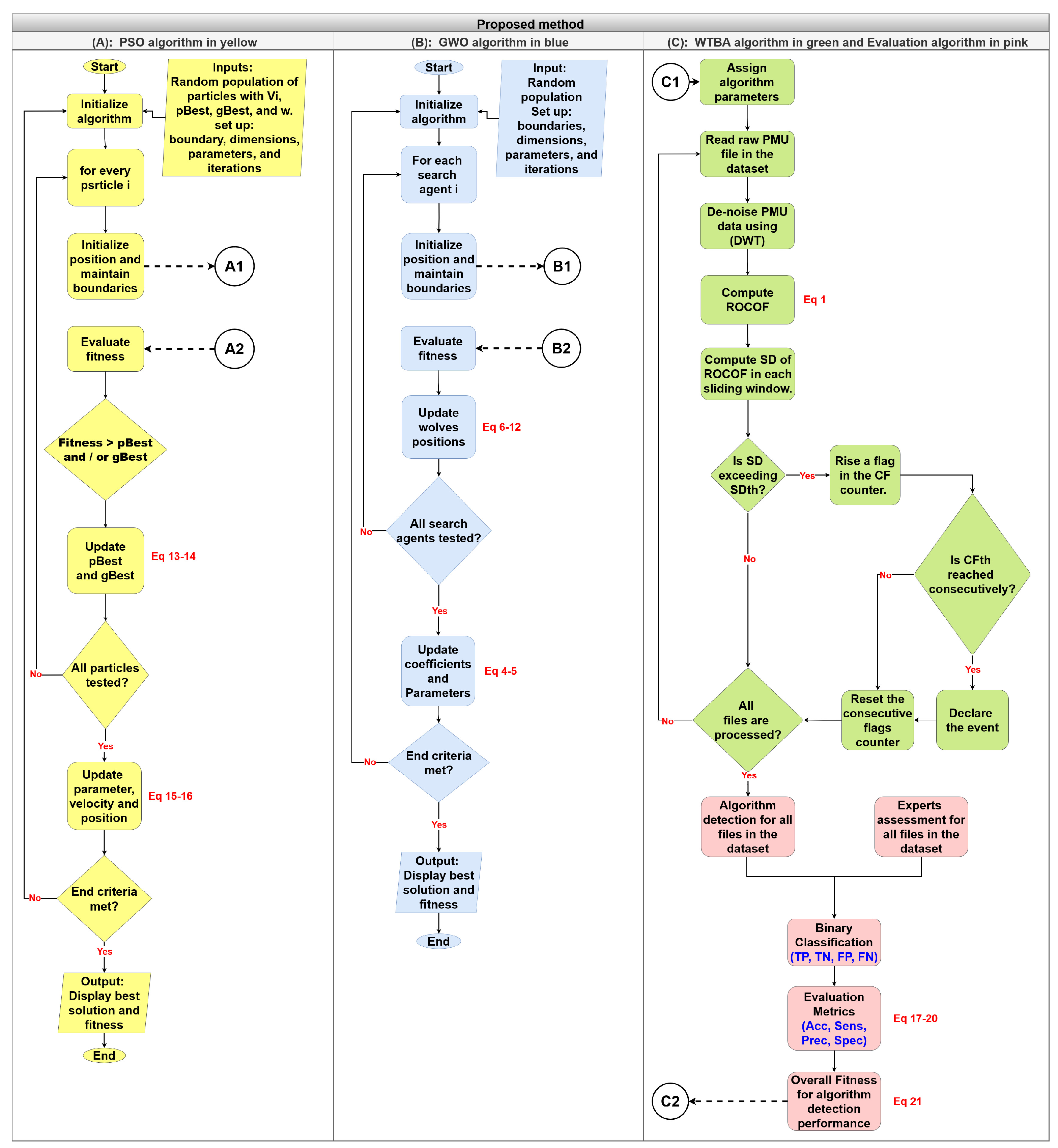
The contributions of this work are organized around four key aspects. First, it enhances the performance of the frequency event detection algorithm by optimizing its parameters across multiple datasets using GWO and PSO. Unlike traditional approaches that rely on equally weighted metrics, our method introduces variable-weighted metrics, leading to superior detection specificity and substantially reducing false event detection.

Second, this study provides a novel, in-depth analysis of the impact of different metrics on event detection performance. It also introduces a new framework for quantifying frequency non-event incidents in power systems, an aspect often overlooked in conventional methodologies.

Third, this study identifies the optimal search agents and particles for GWO and PSO by systematically evaluating fitness scores, computational time, and convergence speed, ensuring robust and efficient parameter selection for frequency event detection.

Finally, this work provides a comprehensive and visually intuitive representation of how optimization techniques integrate into frequency detection algorithms, serving as a valuable foundation for future research and advancements in this evolving domain.

The paper is structured as follows: Section 2 outlines the methodology, Section 3 presents the proposed variable weighted metrics methodology, Section 4 introduces four case studies, Section 5 discusses the results, and Section 6 concludes with future directions.

2. Methodology

The methodology of this work introduces four key components: frequency event detection algorithm (WTBA), optimization techniques (GWO and PSO), performance evaluation methods, and the visual representation of optimization method integration. Each of these aspects is explored in detail in the following subsections.

2.1. Frequency Event Detection Algorithm

The WTBA employs a hybrid approach, wherein signal processing and statistical methods are combined to detect frequency events. At its core, the algorithm uses four key parameters that work in tandem to identify significant frequency deviations.

Window Size (WS): This parameter influences the computation of the standard deviation (SD) within each analysis window derived from the ROCOF dataset, meaning that a larger window size naturally results in a higher SD value. A larger Window Size (WS) enhances the overall smoothness of the ROCOF signal by averaging out short-term fluctuations, which improves binary classification and reduces incorrect event declarations. However, using an excessively large window can increase processing time and risk over-integrating the data, further elevating the SD. Conversely, a smaller window captures more transient variations, potentially introducing noise that may compromise the reliability of event detection.

Frequency Measurements Difference (FMD): This represents the separation gap between successive frequency measurements that are used to compute the ROCOF. This parameter affects both the ROCOF and the SD by defining the time interval over which frequency changes are observed. Increasing the Frequency Measurements Difference (FMD) leads to a higher absolute ROCOF value and produces a smoother signal profile, which is beneficial for accurate event detection. However, straying from the optimal FMD value can disrupt the balance between capturing rapid frequency changes and achieving a smooth signal, thereby degrading the algorithm’s performance.

Standard Deviation Threshold (SDth): The SDth is pivotal because it determines the level at which a true flag is raised—when the SD exceeds this threshold, a flag is triggered, and a series of such flags may culminate in an event declaration. Careful tuning of Standard Deviation Threshold (SDth) is essential: setting it too high may lead to missed detections (false negatives), while setting it too low can result in spurious detections (false positives). Experimental evaluations have shown that maintaining an optimal SDth is critical for the overall reliability of the algorithm.

Consecutive Flags Threshold (CFth): This parameter specifies the number of successive true flags required to confirm an event once the SD is exceeded. Its value is crucial for accurately distinguishing genuine events from noise. Deviations from the optimal Consecutive Flags Threshold (CFth) can negatively impact performance by increasing the likelihood of either false positives or false negatives, as observed in experimental assessments. Further elaboration on the WTBA can be found in prior works [4,5].

The algorithm operates in two sequential stages: signal processing and then statistical analysis, as illustrated in Algorithm 1. In the signal processing stage, the incoming frequency data undergo a noise elimination process using DWT, which removes the measurement noise while maintaining the signal characteristics. In the statistical stage, however, the denoised frequency data are processed by computing the ROCOF.

$$\mathrm{ROCOF}\left(t\right)={\displaystyle \frac{f_t-f_{t-1}}{\Delta t}}$$

(1)

where $f_t$ and $f_{t-1}$ are consecutive, discrete frequency measurements and $\Delta t$ denotes their time interval. The mean, variance, and standard deviation of the ROCOF dataset are then computed over the sliding window to identify potential events based on the thresholds.

Algorithm 1 Wavelet Transform-Based Algorithm

1: Start   2: Read PMU data.   3: Set algorithm parameters.   4: Main Loop:   5: for each frequency measurement do   6:       Denoise frequencies.   7: end for   8: for each denoised frequency measurement do   9:       Calculate ROCOF. (Equation (1)) 10: end for 11: for each sliding window over ROCOF do 12:       Calculate $\overline{x}$, Var, and SD. 13:       if SD > SDth then 14:             Add 1 to high SD counter. 15:       end if 16:       if high SD counter > CFth then 17:             Declare event. 18:             Reset high SD counter. 19:       end if 20: end for 21: End Main Loop 22: End

2.2. Optimization Techniques

This research employs two nature-inspired optimization methods, i.e., GWO and PSO, to enhance the WTBA algorithm’s parameters selection. These methods are reviewed regarding their inspiration, mathematical formulations, and pseudocode representations.

2.2.1. Grey Wolf Optimization (GWO)

The GWO algorithm, introduced by Mirjalili et al. in 2014, belongs to the category of swarm-intelligence-based algorithms [27]. It derives inspiration from the hunting strategy and social structure observed in grey wolves. These animals exhibit social dynamics characterized by packs with a clear hierarchical structure divided into four levels: $\alpha$, $\beta$, $\delta$, and $\omega$.

The $\alpha$ wolves represent the group’s command, making decisions and directing the pack’s actions, embodying the most optimal solution. $\beta$ wolves support $\alpha$ wolves in decision making, supervise other pack members, and serve as replacements when needed, representing the second-best solutions. $\delta$ wolves rank below $\alpha$ and $\beta$ wolves but above $\omega$ wolves, supervised by $\alpha$ and $\beta$ wolves, and represent the third-best solutions. $\omega$ wolves occupy a lower hierarchical level, following the lead of higher-ranked wolves and serving as additional candidate solutions.

The wolf pack’s hunting process involves three primary stages: pursuit, encirclement of the prey, and the actual attack. Initially, a predetermined number of wolves, acting as search agents, have their positions randomly generated. The encircling behavior begins by calculating the distance $\overrightarrow{D}$ between each grey wolf and the prey, the optimal solution. Subsequently, the position ${\overrightarrow{X}}^{t+1}$ of each wolf is updated in the next iteration using the following equations:

$$\overrightarrow{D}=|\overrightarrow{C}{\overrightarrow{X_p}}^t-{\overrightarrow{X}}^t|$$

(2)

$${\overrightarrow{X}}^{t+1}={\overrightarrow{X_p}}^t-\overrightarrow{A}\overrightarrow{D}$$

(3)

where $\overrightarrow{X}$ represents the wolf’s position and $\overrightarrow{X_p}$ denotes the prey’s position, where t and $t+1$ represent the current and the following iteration, respectively. Additionally, $\overrightarrow{A}$ and $\overrightarrow{C}$ are coefficient vectors obtained from the following equations:

$$\overrightarrow{A}=2a{r}_1-a$$

(4)

$$\overrightarrow{C}=2r_2$$

(5)

The value of a linearly decreases from 2 to 0 throughout the iterations, while $r_1$ and $r_2$ denote random numbers ranging from 0 to 1. During the optimization process, the positions of $\omega$ wolves are recalibrated around $\alpha$, $\beta$, and $\delta$. Guided by these values, $\omega$ wolves undergo repositioning. The updated mathematical models for the wolves’ positions start by calculating the distances to $\alpha$, $\beta$, and $\delta$ as follows:

$$\overrightarrow{D_{\alpha }}=|\overrightarrow{C_1}\overrightarrow{X_{\alpha }}-\overrightarrow{X}|$$

(6)

$$\overrightarrow{D_{\beta }}=|\overrightarrow{C_2}\overrightarrow{X_{\beta }}-\overrightarrow{X}|$$

(7)

$$\overrightarrow{D_{\delta }}=|\overrightarrow{C_3}\overrightarrow{X_{\delta }}-\overrightarrow{X}|$$

(8)

where $\overrightarrow{X_{\alpha }}$, $\overrightarrow{X_{\beta }}$, and $\overrightarrow{X_{\delta }}$ denote the positions of $\alpha$, $\beta$, and $\delta$, respectively, while $\overrightarrow{C1}$, $\overrightarrow{C2}$, and $\overrightarrow{C3}$ stand for the relevant coefficient vectors. The symbol $\overrightarrow{X}$ denotes the current solution position vector. Subsequently, the positions of the $\omega$ wolves are updated based on the average values of $\alpha$, $\beta$, and $\delta$.

$$\overrightarrow{X_1}=\overrightarrow{X_{\alpha }}-\overrightarrow{A_1}\overrightarrow{D_{\alpha }}$$

(9)

$$\overrightarrow{X_2}=\overrightarrow{X_{\beta }}-\overrightarrow{A_2}\overrightarrow{D_{\beta }}$$

(10)

$$\overrightarrow{X_3}=\overrightarrow{X_{\delta }}-\overrightarrow{A_3}\overrightarrow{D_{\delta }}$$

(11)

where $\overrightarrow{A_1}$, $\overrightarrow{A_2}$, and $\overrightarrow{A_3}$ are coefficient vectors and $\overrightarrow{X_1}$, $\overrightarrow{X_2}$, and $\overrightarrow{X_3}$ represent position vectors calculated based on the locations of $\alpha$, $\beta$, and $\delta$, respectively, indicating a closer position for $\omega$ in relation to the position of the three dominant wolves. The average of these position vectors yields an optimal new position for the remaining $\omega$ wolves, as depicted in the following function.

$${\overrightarrow{X}}^{t+1}={\displaystyle \frac{\overrightarrow{X_1}+\overrightarrow{X_2}+\overrightarrow{X_3}}{3}}$$

(12)

This averaging strategy ensures each search agent converges towards the prey, the best solution, representing exploitation while maintaining the flexibility to explore alternative regions. In essence, this mechanism balances exploration and exploitation within the optimization process. The GWO algorithm process is detailed in Algorithm 2.

2.2.2. Particle Swarm Optimization (PSO)

The PSO algorithm was proposed by Russell Eberhart and James Kennedy [28]. The method draws inspiration from the swarming and foraging behavior of fish schools and bird flocks. Moreover, particles synchronize their movements in these swarms by adjusting based on neighbors to avoid collisions and overcrowding. They align with the group and reach destinations collectively, maintaining distance, matching velocity, and moving towards their neighbors’ average position.

Algorithm 2 Grey Wolf Optimization

1: Start   2: Initialize population, dimensions, boundaries, and iterations.   3: Initialize parameters: a, A, C, and positions for search agents.   4: Main Loop:   5: for each search agent in each iteration do   6:       Define search space limits and handle boundary conditions.   7:       Calculate fitness.   8:       Update wolves positions (Equations (6–12)).   9: end for 10: Update algorithm parameter a. 11: for each search agent do 12:       Update $r1$ and $r2$ randomly within [0-1]. 13:       Update coefficients and parameters (Equations (4–5)). 14: end for 15: if end criteria is met then 16:       Terminate loop. 17: end if 18: End Main Loop 19: Return the best position and fitness score of $\alpha$. 20: End

In PSO, each particle represents a potential solution characterized by three vectors, i.e., position $\overrightarrow{x_i}$, velocity $\overrightarrow{v_i}$, and previous best position $\overrightarrow{pBes{t}_i}$, each with a dimension D corresponding to the search space. The algorithm begins by initializing a random value for a population of particles within the search space. During each iteration, particles assess their positions using an objective function. When a particle improves upon its previous best position, $\overrightarrow{pBes{t}_i}$ is updated, and its corresponding fitness score is recorded in $pBestScor{e}_i$. The swarm’s optimal position, $\overrightarrow{gBest}$, represents the global best solution and updates iteratively if improved. In iteration $t+1$, the values for $pBes{t}_i$ and $gBest$ are obtained using Equations (13) and (14).

$${\overrightarrow{pBes{t}_i}}^{t+1}=\left\{\begin{array}{c}{\overrightarrow{x_i}}^{t+1},ifFitness>{\overrightarrow{pBes{t}_i}}^t\hfill \\ {\overrightarrow{pBes{t}_i}}^t,ifFitness\le {\overrightarrow{pBes{t}_i}}^t\hfill \end{array}\right.$$

(13)

$${\overrightarrow{gBest}}^{t+1}=\overrightarrow{pBes{t}_i}\left(MaxFitness\right),for1\le i\le N$$

(14)

where N is the size of the swarm. After updating particles with the best positions, the velocity is added to the current position of each particle, redirecting the particle in the search space. The velocity vector is computed using Equation (15), and subsequently, particle movement depends on Equation (16).

$${\overrightarrow{v_i}}^{t+1}=w{\overrightarrow{v_i}}^t+c_1.r_1^t({\overrightarrow{pBes{t}_i}}^t-{\overrightarrow{x_i}}^t)+c_2.r_2^t({\overrightarrow{gBest}}^t-{\overrightarrow{x_i}}^t)$$

(15)

$${\overrightarrow{x_i}}^{t+1}={\overrightarrow{x_i}}^t+{\overrightarrow{v_i}}^{t+1}$$

(16)

where w is referred to as the inertia coefficient, $c_1$ and $c_2$ are constants known as acceleration coefficients, and $r_1$ and $r_2$ are random numbers in the range from 0 to 1. The velocity is computed individually for each particle in every dimension.

There are three components influencing the movement of each particle i, i.e., inertia, cognitive, and social, as follows:

• The inertia component maintains the particle’s current motion direction, computed as $w{\overrightarrow{v_i}}^t$ and governed by the parameter w.
• The cognitive component drives particles towards previously encountered best positions, computed as $c_1{r}_1^t({\overrightarrow{pBes{t}_i}}^t-{\overrightarrow{x_i}}^t)$ and controlled by $c_1$.
• The social component guides particles towards the successful positions of other particles, computed as $c_2{r}_2^t({\overrightarrow{gBest}}^t-{\overrightarrow{x_i}}^t)$ and regulated by $c_2$.

Equation (15) illustrates the linear sum of these three components. The implementation process of PSO is detailed in Algorithm 3.

Algorithm 3 Particle Swarm Optimization

1: Start   2: Initialize population, dimensions, boundaries, and iterations   3: Initialize parameters: $v_{max}$, $w_{Max}$, $w_{Min}$, $c_1$, and $c_2$   4: for each particle do   5:       Randomly initialize velocity and position   6:       Calculate fitness   7: end for   8: Initialize $pBest$ and $gBest$   9: Main Loop: 10: for each search agent in each iteration do 11:       Define search space limits and handle boundary conditions 12:       Update $pBest$ and $gBest$. (Equations (13–14)) 13: end for 14: Update w 15: for each search agent in each iteration do 16:       Update parameters, velocities, and positions. (Equations (15–16)) 17: end for 18: if end criteria is met then 19:       Terminate 20: end if 21: End Main Loop 22: Return global best fitness and position 23: End

2.3. Performance Evaluation Methods

A comprehensive evaluation framework was developed to assess the detection algorithm’s performance. The framework incorporates four key tools: dataset procurement, experts’ evaluation, binary classification, and evaluation metrics. This integrated approach enables thorough validation of the algorithm’s effectiveness across various frequency datasets.

2.3.1. Datasets Procurement

The frequency response test station (FRTS) serves as the primary source of PMU data, facilitating automated data acquisition, processing, and archival operations. The station incorporates a PMU, real-time automation controller (RTAC), and Global Positioning System (GPS) clock working in tandem. The PMU transmits synchrophasor measurements to the RTAC at a rate of 30 samples per second, with data archived as CSV files containing 18,000 samples per 10-min segments. These files undergo systematic extraction by the research team and comprehensive analysis afterward.

According to North American Electric Reliability Corporation (NERC), frequency events are typically classified as under-frequency events and over-frequency events, which result from a significant loss or change of generation or load, respectively [2]. Additionally, major faults can contribute to these events. Since the loss of a large generator is much more likely than a sudden change in an equivalent amount of load, under-frequency events are more commonly discussed and emphasized in the context of frequency event detection.

The selection of datasets in this study was guided by the need for a diverse and comprehensive representation of frequency events across various grid conditions. To ensure a broad spectrum of event types for validation purposes, the datasets were designed to include both under-frequency and over-frequency events. This classification was performed through expert evaluation for frequency events and quasi-events visualizations, then confirmed using the NERC annual frequency report.

Furthermore, dataset selection considered variations in system operating conditions, ensuring the methodology remains applicable across different grid scenarios. Incorporating these factors enhances the generalizability and credibility of the experimental results.

2.3.2. Experts’ Evaluation

Characterizing frequency events presents unique challenges due to system-specific factors [29]. Therefore, on a weekly basis, power system experts conduct weekly assessments of archived PMU frequency data from the test station to address this complexity. These data include non-events, quasi-events (not-so-obvious), and events, as shown in Figure 1A, B, and C, respectively.

These figures provide a comparative visualization of three types of frequency deviation observed over 18,000 samples (10 min) from the Western Interconnection, USA. Plot A illustrates a non-event scenario where the frequency remains stable around the nominal value. In contrast, Plot B captures a quasi-event, characterized by a transient frequency drop. Finally, Plot C depicts a confirmed under-frequency event reported by NERC, where the frequency exhibits a sharp and deep decline to a critical level.

The experts categorize these samples as event or non-event incidents, providing a reference for evaluating detection algorithm efficacy. Another benefit of applying expert evaluation to historical PMU frequency data is the ability to analyze the variation and distribution of events and quasi-events over time.

Figure 2 presents a heat map illustrating the monthly distribution of detected frequency events and quasi-events from 2019 to 2023. This visualization reveals temporal trends in frequency disturbances, enabling researchers to identify periods of heightened system instability and assess seasonal or operational influences on grid frequency dynamics.

2.3.3. Binary Classification and Evaluation Metrics

The algorithm’s performance is evaluated through binary classification metrics that compare its outputs against the expert assessments using:

• True Positive (TP): Event detected by both the experts and the algorithm.
• True Negative (TN): Agreement between the experts and the algorithm that no event occurs.
• False Positive (FP): The algorithm incorrectly identifies an event that experts did not recognize.
• False Negative (FN): The algorithm fails to detect an event that was identified by the experts.

From these binary classification results, four key performance metrics are derived to quantify the effectiveness of the detection algorithm performance. These metrics are:

• Accuracy: Quantifies the successful identification of both events and non-events against all events and non-events within the set.

  $$Accuracy={\displaystyle \frac{TP+TN}{SetSize}}\times 100\%$$

  (17)
• Sensitivity: Quantifies the successful identification of events against all events within the set.

  $$Sensitivity={\displaystyle \frac{TP}{TP+FN}}\times 100\%$$

  (18)
• Precision: Quantifies the successful identification of events against all identified events.

  $$Precision={\displaystyle \frac{TP}{TP+FP}}\times 100\%$$

  (19)
• Specificity: Quantifies the successful identification of non-events against all non-events within the set.

  $$Specificity={\displaystyle \frac{TN}{TN+FP}}\times 100\%$$

  (20)

2.4. Integration of Optimization Methods

The previous subsections detailed the WTBA algorithm, optimization techniques, and performance evaluation methods as individual components. This section, however, describes how these components are integrated into a cohesive framework for parameter optimization. This integration enables systematic parameter tuning through optimization feedback loops, allowing the WTBA algorithm’s performance to be iteratively refined until convergence or the satisfaction of predefined criteria.

The proposed methodology integrates optimization techniques with the WTBA algorithm through a systematic data exchange framework illustrated in Figure 3. The framework consists of four interlinked components: PSO (yellow), GWO (blue), the WTBA algorithm (green), and the evaluation methods (pink). These components exchange data through dedicated ports (A1, A2, B1, B2, C1, and C2) to facilitate the optimization process. The optimization process is guided by an objective function that combines four key metrics, as shown in Equation (21).

$$\mathrm{Max}(Accuracy+Sensitivity+Precision+Specificity)$$

(21)

Figure 3 depicts the interaction between the optimization algorithms and the WTBA framework. The PSO (yellow) and GWO (blue) algorithms adjust their parameters through data exchange with the WTBA (green), guided by feedback from the evaluation method (pink). This iterative process ensures the continuous improvement of WTBA performance in detecting frequency events.

The data exchange process can be implemented using either PSO or GWO as the optimization methods. For the PSO algorithm, the algorithm generates particle positions, which flow from port A1 to the WTBA through port C1 as a set of parameters. Following detection and performance evaluation, the fitness scores are returned via port C2 to PSO through port A2. Within the PSO, these fitness scores are compared against the current scores to update the new particle positions for the next iteration.

The GWO integration follows a similar process. The algorithm generates wolf positions as a set of parameters. These parameters are transferred from port B1 to the WTBA through port C1. After completing the detection and evaluation process, the fitness scores are computed and sent back from port C2 to the GWO through port B2. The GWO then compares the fitness score with the previous score to update the optimization process for optimal WTBA parameters. This bidirectional flow of information ensures continuous refinement of algorithm parameters while maintaining the balance between exploration and exploitation in the optimization process.

3. Proposed Methodology of Variable Weighted Metrics

This section introduces the variable weighted metrics methodology, emphasizing specificity’s role in detection performance and its relation to frequency non-event quantification. Given the impact of false positives, we examine the interplay between specificity and sensitivity before proposing a novel approach to enhance detection algorithm reliability using real-world data.

3.1. Balancing Specificity and Sensitivity Metrics

Specificity and sensitivity, along with other performance metrics, form the foundation of the binary classification framework, where events must be accurately distinguished from non-events. However, the conventional approach of treating these metrics equally fails to account for a fundamental characteristic of power system events: their inherent class imbalance. In real-world operations, frequency events are rare, while normal fluctuations reflect quasi-events or non-events.

Balanced classes refer to situations where the number of cases in each class is approximately equal. In such scenarios, metrics like accuracy provide a meaningful evaluation of system performance. In contrast, imbalanced classes describe situations where one class significantly outweighs the other. This is typical in frequency event detection for power systems, where events occur rarely, while non-events, including quasi-events, happen routinely. In these instances, accuracy may not provide a comprehensive evaluation, and the focus shifts to specificity and sensitivity to minimize misclassifications. Therefore, FP takes higher priority, while FN is less critical.

In frequency event detection and response, specificity is critical, as it prioritizes accurate identification of non-event incidents and minimizes FP cases. An increase in FPs represent incorrect identifications or false alarms of events that are not actually happening. Frequency response applications are sensitive to FPs because they can trigger unnecessary grid services, leading to operational disruptions and additional costs associated with unwarranted frequency support actions.

FN cases indicate that the algorithm failed to detect an actual event, thereby reducing the precision of its detection performance. Given the rarity of real events, automatic frequency control actions, in conjunction with protection system strategies, can intervene to arrest frequency decline and mitigate its impacts. Consequently, precision holds moderate importance. However, the imbalance between FN and FP likelihoods prioritizes specificity, as FPs negatively impact system performance and lead to higher costs.

In the context of grid frequency monitoring and analysis, sensitivity metrics are of particular importance, especially during the offline analysis of frequency performance. Accordingly, detection algorithms must be calibrated to identify even less severe deviations. This increased sensitivity facilitates the identification of more FP cases, representing potential quasi-event incidents. The significance of quasi-events lies in their ability to serve as challenging cases for testing and evaluating detection algorithm performance, as they share common characteristics with real events but exhibit moderate severity in terms of decline depth and steepness.

In practice, offline analysis is conducted on a weekly basis using a detection algorithm with high sensitivity to process historical frequency deviations. This results in a weekly report of potential events, including both real events and quasi-events, which are then subject to expert assessment. These assessments aim not only to detect real events but also to evaluate potential quasi-events for further analysis.

Thus, specificity plays a pivotal role in the detection phase, where minimizing FPs is crucial to prevent unnecessary grid services and mitigate operational disruptions. Striking a balance between specificity and other metrics, such as sensitivity, ensures the system’s overall reliability and cost-effectiveness. In the monitoring phase, which prioritizes the identification of even minor deviations to detect challenging quasi-event incidents, these cases provide valuable opportunities to assess and refine the algorithm’s detection performance. Collectively, the detection and monitoring phases contribute to the algorithm’s effectiveness in maintaining the reliability of the power system.

3.2. Quantitative Analysis of Non-Events: A Specificity-Driven Approach

This subsection provides an overview of the methodology employed for estimating non-event incidents, specifically applied to data spanning from 2019 to 2023. It begins by calculating the duration of a single frequency event according to NERC and the total annual duration of all events during the study period. From these, the potential number of non-event incidents is derived [2]. The impact of reduced specificity scores (<100%) on detection performance is examined. The relevant equations for these calculations will be presented and applied throughout this analysis, providing key insights into the reliability of detection methods and system stability evaluation.

$$T_{\mathrm{year}}=365\times 24\times 60\times 60=31,536,000\mathrm{s}$$

(22)

where $T_{\mathrm{year}}$ represents the total number of seconds in a year, which is computed by multiplying the number of days, hours, minutes, and seconds.

$$t_{\mathrm{event}}=20+32=52\mathrm{s}$$

(23)

where $t_{\mathrm{event}}$ is the total duration of a single event as per [2], (t₀ − t + 52), consisting of an approximate 20 s duration related to the time between value A and value B, and a 32 s duration related to value B, where we combine them to obtain the total time span.

$$T_{\mathrm{events}}=N_{\mathrm{events}}\times t_{\mathrm{event}}$$

(24)

where $T_{\mathrm{events}}$ is the total time occupied by events in a year, which is calculated as the product of the number of events ($N_{\mathrm{events}}$) and the duration of a single event ($t_{\mathrm{event}}$).

$$T_{\mathrm{non}\text{-}\mathrm{events}}=T_{\mathrm{year}}-T_{\mathrm{events}}$$

(25)

where $T_{\mathrm{non}\text{-}\mathrm{events}}$ represents the total time in a year not occupied by events, here derived by subtracting the total event time $T_{\mathrm{events}}$ from the total year time $T_{\mathrm{year}}$.

$$N_{\mathrm{non}\text{-}\mathrm{events}}={\displaystyle \frac{T_{\mathrm{non}\text{-}\mathrm{events}}}{t_{\mathrm{event}}}}$$

(26)

where $N_{\mathrm{non}\text{-}\mathrm{events}}$ is the total number of possible non-event incidents in a year, which is computed by dividing the total non-event time $T_{\mathrm{non}\text{-}\mathrm{events}}$ by the duration of a single event $t_{\mathrm{event}}$.

$$Potential\left(\mathrm{FP}\right)={\displaystyle \frac{\mathrm{TN}}{\mathrm{Specificity}}}-\mathrm{TN}$$

(27)

where FP represents the potential number of false positives, here calculated using the number of true negatives (TN) and the specificity value from Equation (20).

For further clarification, this methodology, along with the corresponding equations, is applied to real frequency event incidents reported by NERC from 2019 to 2023 to estimate the possible number of non-event cases. Various hypothetical specificity ratios are then analyzed to illustrate the critical impact of reduced specificity on the rise in false positives. The process begins by determining the confirmed event count for each year, followed by estimating potential non-events. Finally, the projected false positive incidents are calculated using different specificity ratios, as detailed in

Table 2. Event and non-event metrics for various years.

Year	Events	Tevents (24)	Tnon-events (25)	Nnon-events (26)	Hypothetical Specificity	Potential (FP) (27)
2019	20	1040	31,534,960	606,442	1	0
2020	19	988	31,535,012	606,443	0.9999	61
2021	23	1196	31,534,804	606,439	0.999	607
2022	20	1040	31,534,960	606,442	0.99	6126
2023	24	1248	31,534,752	606,438	0.9	67,382

.

While the specificity ratios are employed solely to illustrate the methodological framework, they demonstrate how even slight incremental reductions in specificity (sixth column) can substantially increase FP cases (seventh column). The table underscores the trade-off between specificity and FP occurrences, offering insights into the challenges of maintaining high specificity in event detection systems.

3.3. Integration of Variable Weighted Metrics

The proposed methodology enhances the WTBA algorithm by incorporating variable weighted metrics into the optimization objective function. Unlike conventional methods that assign equal weights to all detection metrics, this approach prioritizes specificity—the algorithm’s ability to identify true negatives (frequency non-event incidents)—to minimize FP.

To achieve this, the original objective function, as defined in Equation (21), is modified to incorporate variable weights for Accuracy, Sensitivity, Precision, and Specificity, as shown in Equation (28).

$$max\left(\mathrm{Accuracy}·w_1+\mathrm{Sensitivity}·w_2+\mathrm{Precision}·w_3+\mathrm{Specificity}·w_4\right)$$

(28)

where $w_1$, $w_2$, $w_3$, and $w_4$ represent the relative weights reflecting the importance degree assigned to each metric. By increasing the weight of specificity, the methodology reduces false positives, while possible compromising on other metrics, particularly sensitivity and precision. This trade-off is especially relevant in practical applications, where misclassifying normal frequency fluctuations as events could trigger unnecessary control actions.

Table 3. Various weight sets used for each metric.

Weight Sets	Set 1	Set 2	Set 3	Set 4	Set 5	Set 6	Set 7	Set 8	Set 9	Set 10	Set 11	Set 12
Accuracy	0.1	0.1	0.1	0.1	0.05	0.05	0.01	0.1	0.2	0	0	0
Sensitivity	0.1	0.2	0.4	0.1	0.3	0.2	0.01	0.3	0.2	0.3	0.2	0.1
Precision	0.4	0.3	0.1	0.3	0.05	0.05	0.01	0.1	0.2	0	0	0
Specificity	0.4	0.4	0.4	0.5	0.6	0.7	0.97	0.5	0.4	0.7	0.8	0.9

presents different weight sets used to evaluate the impact of prioritizing specificity. The optimal set is determined by analyzing the detection algorithm’s performance, particularly specificity improvement, across small- and large-scale datasets, as illustrated in the third and fourth case studies in Section 4 and Section 5.

4. Case Studies

The systematic evolution of the proposed methodology is conducted through four interconnected, progressive case studies, each designed to assess specific aspects of the WTBA algorithm’s performance. The first two case studies determine the optimal number of search agents/particles in GWO and PSO, while the latter two demonstrate the effectiveness of variable-weighted metrics against conventional methods.

The first case study investigates the impact of varying the number of search agents in GWO and PSO optimization techniques, focusing on fitness score, convergence, and computational efficiency. This foundational investigation is crucial as its optimal agent/particle configuration results directly apply to the subsequent second and third studies, since they process the same datasets illustrated in

Table 4. PMU Frequency data in each small-scale dataset.

Dataset	Event	Quasi-Event	Non-Event
30 files dataset in [5]	13	6	11
60 files dataset in [4]	6	34	20
70 files dataset	12	38	20

.

The second case study builds on these optimization findings, using established optimal configurations to tune the WTBA algorithm parameters (WS, FMD, SDth, and CFth). This study compares the WTBA’s performance using these optimized parameters against estimated parameters from prior research [4,5].

The third case study introduces the concept of weighted metrics through two sequential phases. The first phase establishes a baseline by comparing the detection performance of WTBA and LSLR [6] using the conventional method of equally weighted metrics, as defined in Equation (21), by processing the three small-scale datasets listed in Table 4. The second phase then further improves detection specificity for both algorithms by applying the proposed method of variable-weighted metrics, depicted in Equation (28).

The fourth case study extends this weighted metrics approach to a large-scale validation, applying both algorithms (WTBA and LSLR) to extensive PMU datasets spanning four months of power system operation, as shown in

Table 5. PMU Frequency data in each large-scale dataset.

Period	Total Files	Events	Quasi-Events	Non-Events
September 2020	4236	5	4	4227
July 2021	4402	3	4	4395
April 2023	4082	4	4	4074
October 2023	4404	2	3	4399

. This final case validates the scalability of the variable-weighted metrics methodology in real-world applications, processing thousands of files of frequency measurements while maintaining the optimal detection specificity.

Each month includes a sufficient number of events confirmed by NERC, quasi-events identified by experts, and routine frequency non-events. The distribution of these events and quasi-events, illustrated in the heatmap in Figure 2, informs the systematic selection of the analyzed months. The inclusion of the entire frequency PMU data from these four months validates the WTBA algorithm’s detection performance with the variable weighted metrics approach, suggesting its potential for deployment in online applications in the next development phase, as discussed in Section 6.

5. Results and Discussion

This section discusses the results of the four studies. The first study determines the optimal number of search agents and particles. The second compares the detection performance of WTBA with estimated versus optimized parameters. The third and fourth studies compare the detection performance of WTBA and LSLR using equally versus variable weighted metrics, processing small-scale and large-scale datasets, respectively.

A summary of the tables used to present the results of these studies is shown in

Table 6. Summary of results tables.

Case Study	Table	Description
First	7	Best fitness scores
	8	Best convergence iterations
	9	Best computational time
Second	10	WTBA detection performance using estimation vs. optimized parameters
Third	11	WTBA vs. LSLR using equal weighted metrics
	12	WTBA and LSLR: equal vs. variable weighted metrics on small-scale datasets
Fourth	13–16	WTBA and LSLR: equal vs. variable weighted metrics on large-scale datasets

. This table outlines the case studies, corresponding tables, descriptions, and key insights that are further elaborated upon in the following subsections.

5.1. First Case Study

From

Table 7. Best fitness score.

Algorithm	Dataset	Search Agents/Particles
		5	10	20	30	40
GWO	30 files	372	372	372	372	372
	60 files	382	382	382	382	382
	70 files	380	380	380	380	380
PSO	30 files	356	356	372	372	372
	60 files	382	382	382	382	382
	70 files	380	380	371	380	380

, applying the GWO technique to datasets of 30, 60, and 70 files improved fitness scores of the WTBA algorithm to 372, 382, and 380, respectively. However, changing the number of search agents did not uniformly enhance detection performance across all datasets. Thus, selecting the smallest number of agents remains optimal, ensuring consistent results even with increased search agents.

The PSO method improved the WTBA fitness scores to 372, 382, and 380 for datasets of 30, 60, and 70 files, respectively, irrespective of particle count. However, with 30 files, a lower particle count led to a score of 356. Moreover, using 20 particles with the 70-file dataset resulted in a score of 371, contrasting with the score of 380 obtained with other particle counts. Thus, using 30 particles consistently yields the highest fitness score across all datasets.

Comparing GWO and PSO for enhancing fitness scores of the WTBA performance, GWO consistently yielded better results regardless of search agents. In contrast, using 30 search agents with PSO yielded optimal scores across all datasets. Therefore, using GWO with a smaller number of search agents, specifically five, emerged as the best option to provide the best fitness score. While the overall fitness score is not the most efficient criterion for sensitively analyzing detection performance, particularly when compared to metrics such as specificity, it can still serve as an indicative measure of improvement when optimizing with varying numbers of search agents or particles.

Table 8. Convergence to optimal results.

Algorithm	Dataset	Search Agents/Particles
		5	10	20	30	40
GWO	30 files	12	13	3	4	1
	60 files	1	4	1	1	1
	70 files	18	14	3	4	4
PSO	30 files	14	16	15	2	3
	60 files	7	1	1	1	1
	70 files	17	6	1	4	4

presents the iteration number at which the GWO and PSO optimization techniques converge to the optimal solution, achieving the best fitness score across various search agents or particle numbers. Generally, fewer search agents or particles require more iterations for the optimization techniques to achieve the optimal score. Specifically, in the 30-file dataset, GWO achieved the best score earlier than PSO with 5 and 10 search agents due to its higher fitness score. Similarly, in the 60-file datasets, both techniques converged to the best score within the first iteration, except with 10 search agents in GWO and 5 particles in PSO. However, in the 70-file dataset, the iteration number required to attain the optimal fitness score varied between GWO and PSO.

Table 9. Computational time (in minutes).

Algorithm	Dataset	Search Agents/Particles
		5	10	20	30	40
GWO	30 files	76	167	324	361	577
	60 files	234	342	810	1026	1584
	70 files	276	540	756	1128	1164
PSO	30 files	56	121	258	364	561
	60 files	252	288	756	882	1284
	70 files	270	354	678	1110	1296

summarizes 30 simulations, totaling around 298 h of optimization processing time, with GWO at 156 h and PSO at 142 h. Both methods processed identical datasets with varying numbers of search agents or particles. PSO outpaced GWO in 12 out of 15 instances, while GWO surpassed PSO three times, mainly with 30, 5, and 40 search agents for the 30, 60, and 70-file datasets, respectively. Notably, the difference in computational time between the two techniques ranged from 3 min with 30 agents in the 30-file dataset, where GWO was faster, to 300 min with 40 particles in the 60-file dataset, favoring PSO.

In conclusion, the findings underscore the significance of dataset diversity, particularly the inclusion of challenging quasi-events. The 70-file dataset, which comprises the most diverse combination of files, revealed that GWO consistently achieved a fitness score of 380, while PSO displayed variability, particularly with the 30-file dataset. Fewer search agents or particles resulted in longer convergence times, with the exception of the 60-file dataset, where both GWO and PSO converged more swiftly. Computational efficiency was markedly influenced by the number of agents, with five agents yielding results comparable to 40 agents in significantly less time.

Although achieving a perfect score of 400 remains challenging, GWO with five search agents demonstrates optimal performance, with minimal computational time differences compared to PSO. As a result, the GWO with five search agents is chosen as the preferred approach for the second and third case studies, which analyze the same datasets.

5.2. Second Case Study

In

Table 10. Detection performance comparison of the WTBA algorithm: estimated vs. optimized parameters with equal weighted metrics.

Dataset	30-File Dataset		60-File Dataset		70-File Dataset
Parameter Tuning Type	Estimated in [5]	Optimized	Estimated in [4]	Optimized	Optimized
TP	12	12	4	5	10
FP	3	1	0	0	0
FN	1	1	2	1	2
TN	14	16	54	54	58
Accuracy	87	93	97	98	97
Sensitivity	92	92	67	84	83
Precision	80	92	100	100	100
Specificity	82	94	100	100	100
Fitness Score	341	372	364	382	380

, upon reviewing the performance of the frequency events detection algorithm across three datasets in Table 4, using optimized parameters against estimated parameters with equal weighted metrics, improvements are evident. The fitness score in the 30 files dataset increased from 341 to 372, indicating a 9% improvement. Similarly, in the 60 files dataset, there was an enhancement from 364 to 382, reflecting a 5% improvement. These enhancements signify increased algorithmic effectiveness in both datasets.

The results highlight the 70-file dataset for its greater variability and complexity, containing a higher combination of events and quasi-events compared to the 30- and 60-file sets. Moreover, in the 70-file dataset, the WTBA algorithm consistently performs best. The diverse nature of this dataset provided rich signal data, making it the most informative for analysis.

This study emphasizes enhancing specificity in frequency event detection to minimize false positives and prevent unnecessary activation of frequency response assets, such as inverter-based power injections. High specificity is crucial for distinguishing routine frequency fluctuations and quasi-events from critical events, typically occurring only once or twice a month.

The results indicate a post-optimization specificity increase from 82% to 94% in the 30-file dataset, correctly identifying 16 out of 17 non-event cases compared to 14 in previous works [4,5]. In the 60- and 70-file datasets, the algorithm maintains perfect specificity, achieving 100% precision and eliminating false positives. Notably, this consistency in the 70-file dataset, which includes a more diverse range of files, underscores the algorithm’s reliability despite the higher fitness score required for processing the 60-file dataset.

Further improvements were observed across other detection metrics. In the 30-file dataset, accuracy increased from 87% to 93%, while sensitivity remained at 92% due to a single false negative. For the 60-file dataset, accuracy increased from 97% to 98%, and sensitivity improved from 67% to 83% as false negatives dropped from two to one. The 70-file dataset demonstrated comparable accuracy 97% and sensitivity 83%, despite a greater number of event and quasi-event cases.

5.3. Third Case Study

In this case study, the three datasets presented in Table 4 are processed using the proposed WTBA algorithm and validated against the alternative LSLR algorithm, incorporating equally weighted metrics in the optimization objective function, as defined in Equation (21).

Table 11. Detection performance comparison of LSLR and WTBA algorithms on three different datasets using equal weighted metrics.

Dataset	30-File Dataset		60-File Dataset		70-File Dataset
Algorithm	LSLR	WTBA	LSLR	WTBA	LSLR	WTBA
TP	13	12	6	5	9	10
FP	0	1	0	0	3	0
FN	0	1	0	1	3	2
TN	17	16	54	54	55	58
Accuracy	100	93	100	98	91	97
Sensitivity	100	92	100	84	75	83
Precision	100	92	100	100	75	100
Specificity	100	94	100	100	95	100
Fitness	400	372	400	382	336	380

illustrated that the LSLR exhibits superior performance on the 30- and 60-file datasets. However, as the dataset size increases, the WTBA algorithm surpasses LSLR. By emphasizing specificity—defined as the ability to accurately identify TNs, frequency non-event incidents, which are crucial for detection algorithm performance and power system reliability, LSLR achieves high specificity in smaller datasets (30 files and 60 files). A slight decline in specificity is observed in the 70-file dataset, primarily due to an increase in FPs. In contrast, WTBA consistently maintains high specificity, achieving 100% in both the 60-file and 70-file datasets, indicating that it is less prone to FPs as the dataset size increases. It is important to note that the objective function for optimization, represented by Equation (21), incorporates equally weighted metrics to process the datasets under investigation in this case study.

A key observation in both algorithms’ performance on the 60-file dataset is the absence of false-positive incidents, resulting in an optimal specificity score. Consequently, further investigation is required for the 30- and 70-file datasets, focusing on increasing the specificity weight in the optimization objective functions. Unlike previous studies that employ equally weighted metrics, the weight sets in Table 3 place greater emphasis on specificity over accuracy, sensitivity, and precision, as it is directly associated with false positive occurrences, aiming to enhance the algorithm’s specificity and minimize false positives.

An analysis of the results in

Table 12. Detection performance comparison of WTBA (30 files) and LSLR (70 files) using equal-weighted vs. variable-weighted metrics.

Algorithm (Dataset)	WTBA (30-File Dataset)		LSLR (70-File Dataset)
Weight Set	Equal	Set 7	Equal	Set 7
TP	12	5	9	4
FP	1	0	3	0
FN	1	8	3	8
TN	16	17	55	58
Accuracy	93	73	91	89
Sensitivity	92	38	75	33
Precision	92	100	75	100
Specificity	94	100	95	100
Fitness	372	99	336	99

, comparing variable weighted metrics with the initial set of equally weighted metrics in the objective function for WTBA processing the 30-file dataset and LSLR processing the 70-file dataset, reveals that assigning a higher weight to specificity improves both specificity and precision, achieving ideal scores and effectively eliminating false positive incidents, particularly when using Set 7, as other weight sets did not yield superior outcomes. Furthermore, the sensitivity of both algorithms significantly declined, with WTBA dropping from 92% to 38% and LSLR from 75% to 33% due to their failure to accurately detect true events. Accuracy also decreased, particularly for WTBA (93% to 73%) in comparison to LSLR (91% to 89%). Nevertheless, this degradation can be considered an acceptable trade-off between false positives and false negatives, given the high cost of false positive incidents, representing false alarms that may trigger unnecessary grid services in power systems.

5.4. Fourth Case Study

In this case study, we investigate the importance of using variable weights in the optimization objective function, compared to the equal weights metrics previously used to optimize LSLR [6]. To this end, real grid PMU frequency measurements over extended periods are processed, replacing the three small-scale datasets listed in Table 4 and used in the previous case studies to test and analyze detection algorithm performance.

The study focuses on four large-scale datasets spanning four months, encompassing a mix of frequency events, quasi-events, and non-event incidents that reflect real grid conditions, with a quantifiable occurrence of each type, as illustrated in Table 5. The process begins by identifying all three frequency categories through expert evaluations and periodic frequency event reports, which serve as references for optimizing detection algorithm parameters. The optimization emphasizes specificity over other metrics using the weight sets in Table 3.

This study emphasizes two key points. First, the four metrics were retained without rounding to demonstrate how even minor reductions in specificity can significantly affect false positives, especially with large datasets compared to the smaller ones in Table 4. Second, due to the application of different weights, fitness scores do not sum to 400, as observed with the equal-weighted method, shifting the focus to the analysis of specificity and other metrics rather than the fitness score.

Table 13. Detection performance evaluation of WTBA and LSLR using GWO and PSO with equal and variable weighted metrics on the 4236-file dataset (September 2020, 5 events, 4231 non-events).

Algorithm	LSLR		WTBA
Optimization	GWO	PSO	GWO		PSO
Weight Set	Equal	Equal	Equal	Set 2	Equal	Set 8
TP	5	5	4	4	5	5
FP	1	1	3	0	5	3
FN	0	0	1	1	0	0
TN	4230	4230	4228	4231	4226	4228
Accuracy	99.98	99.98	99.91	99.98	100.00	99.93
Sensitivity	100.00	100.00	80.00	80.00	100.00	100.00
Precision	83.33	83.33	56.67	100.00	50.00	62.50
Specificity	99.98	99.98	99.93	100.00	99.88	99.93
Fitness	383	383	337	83	350	120

summarizes the detection performance of LSLR and WTBA, highlighting specificity results for equally weighted and variable weight sets under GWO and PSO optimization. LSLR, using either GWO or PSO with equal weights, achieves 99.98% specificity, with only one false positive and no false negatives, resulting in 83% precision. On the other hand, WTBA with GWO attains 100% specificity when using weight Set 2, eliminating false positives and achieving an ideal false-positive rate. With PSO, performance improves when using weight Set 8 compared to equal weights, as evident in the reduction of false positives from five to three cases. However, PSO generally results in lower specificity than GWO, reinforcing GWO with weight Set 2 as the superior optimization method for this dataset.

Table 14. Detection performance evaluation of WTBA and LSLR using GWO and PSO with equal and variable weighted metrics on the 4402-file dataset (July 2021, 3 events, 4399 non-events).

Algorithm	LSLR		WTBA
Optimization	GWO	PSO	GWO		PSO
Weight Set	Equal	Equal	Equal	Set 6	Equal	Set 5
TP	2	3	1	3	3	3
FP	0	12	1	0	5	0
FN	1	0	2	0	0	0
TN	4399	4387	4398	4399	4394	4399
Accuracy	99.98	99.73	99.93	100.00	99.89	100.00
Sensitivity	66.67	100.00	33.33	100.00	100.00	100.00
Precision	100.00	20.00	50.00	100.00	37.93	100.00
Specificity	100.00	99.73	99.97	100.00	99.88	100.00
Fitness	367	320	283	100	338	100

extends the analysis by evaluating the performance of detection algorithms using equally versus variably weighted metrics within the same optimization techniques. The results reaffirm that LSLR with GWO maintains near-perfect specificity compared to PSO when using equally weighted metrics. However, WTBA with GWO and PSO achieve higher specificity scores with weight sets 6 and 5, respectively, while eliminating FP and FN incidents, leading to perfect scores across other metrics. In conclusion, incorporating variable weighted metrics within the optimization objective function generally enhances detection performance, particularly improving specificity compared to the baseline scenario with no weights.

In

Table 15. Detection performance evaluation of WTBA and LSLR using GWO and PSO with equal and variable weighted metrics on the 4082-file dataset (April 2023, 4 events, 4078 non-events).

Algorithm	LSLR		WTBA
Optimization	GWO	PSO	GWO		PSO
Weight Set	Equal	Equal	Equal	Set 2	Equal	Set 10
TP	3	3	2	4	4	2
FP	1	1	0	0	5	0
FN	1	1	2	0	0	2
TN	4077	4077	4078	4078	4073	4078
Accuracy	99.95	99.95	99.95	100.00	99.88	99.95
Sensitivity	75.00	75.00	50.00	100.00	100.00	50.00
Precision	75.00	75.00	100.00	100.00	44.00	100.00
Specificity	99.98	99.98	100.00	100.00	99.88	100.00
Fitness	375	375	350	100	344	85

, the detection performance of equally weighted metrics is compared across LSLR and WTBA. WTBA with GWO outperforms LSLR (under both optimization techniques) and WTBA with PSO by eliminating false positives, though it results in two false negatives, leading to perfect specificity and precision scores. However, applying weight set 2 with WTBA using GWO further enhances detection performance, achieving ideal scores across all metrics. Meanwhile, weight set 10 with PSO preserves perfect specificity and precision but reduces the performance sensitivity metric.

Table 16. Detection performance evaluation of WTBA and LSLR using GWO and PSO with equal and variable weighted metrics on the 4404-file dataset (October 2023, 2 events, 4402 non-events).

Algorithm	LSLR		WTBA
Optimization	GWO	PSO	GWO		PSO
Weight Set	Equal	Equal	Equal	Set 1	Equal	Set 4
TP	2	2	2	2	2	1
FP	4	9	2	2	17	2
FN	0	0	0	0	0	1
TN	4398	4393	4400	4400	4385	4400
Accuracy	99.91	99.90	99.95	99.95	99.91	99.98
Sensitivity	100.00	100.00	100.00	100.00	100.00	50.00
Precision	33.33	18.20	50.00	50.00	10.59	35.29
Specificity	99.91	99.80	99.95	99.95	99.61	99.95
Fitness	333	318	350	80	311	76

further supports the findings of the previous tables by evaluating the detection performance of LSLR and WTBA under different optimization techniques, first using equally weighted metrics. WTBA with GWO achieved the best results, primarily due to its lower false positive count (only two) while maintaining no false negatives. This performance surpasses both WTBA with PSO and LSLR under both optimization techniques. Applying variable weighted metrics (set 1) in the optimization objective function of GWO with WTBA yielded results identical to those obtained with equally weighted metrics. However, using weight set 4 in PSO with WTBA significantly improved detection performance by reducing false positives from 17 to just 2, though it introduced 1 false negative. This adjustment preserved the specificity score of GWO while slightly lowering precision.

The analysis across all four tables highlights the significant role of optimization techniques and weighting strategies in enhancing detection performance. LSLR consistently demonstrates high specificity, particularly when optimized with GWO, achieving near-optimal results across various datasets. However, WTBA with GWO outperforms all configurations by effectively minimizing or eliminating false positives and achieving ideal specificity when employing the appropriate weight set. While PSO improves WTBA’s performance under certain weighting strategies, it consistently results in lower specificity compared to GWO. These findings underscore the importance of incorporating weighted metrics to enhance detection accuracy, with GWO emerging as the most effective optimization method, especially when combined with WTBA.

Additionally, as mentioned earlier in Section 3.2, the hypothetical specificity ratio and its implications on the increase in FPs, highlighted in Table 2 (specifically in columns 6 and 7), emphasizes the role of specificity in detection performance. This is demonstrated in the results of the fourth case study, where real PMU data processed from various months, as shown in Table 16, indicate that WTBA using PSO with equal weighting led to an increase in FPs, 17 incidents, as specificity slightly declined to 0.9961. Similarly, in Table 14, LSLR using PSO with equal weighting, where specificity was 0.9973, resulted in 12 FPs. These findings underscore the importance of specificity in algorithm optimization and the impact of slight variations in specificity on the increase in FPs.

Notably, the improvement in specificity comes at the expense of increased false negatives and a reduction in sensitivity, highlighting the inherent trade-off between specificity and sensitivity. Given the significant cost of false positives, which represent erroneous system alarms, this trade-off is deemed beneficial, as it ultimately enhances the detection system’s overall performance and contributes to the reliability of power systems. The weight sets 1, 2, and 6, which provide the best specificity and false positive results, offer a promising foundation. Fine-tuning or optimizing the process of selecting these weight sets could result in a universal weight set applicable to a wide range of datasets, thereby ensuring sustained high specificity in detection performance, particularly in real-time applications.

6. Conclusions and Future Directions

This work enhances the detection performance of the WTBA algorithm by optimizing its parameters through GWO and PSO, employing variable-weighted metrics. The performance of the optimized parameters was systematically evaluated across three small-scale datasets and large-scale datasets from four distinct months, encompassing frequency events, quasi-events, and non-events for comprehensive validation. The study is structured around four case studies.

The first case study identified the optimal number of search agents in GWO and particles in PSO, demonstrating that GWO outperforms PSO with smaller search agents. The second case study compared the detection performance of the WTBA algorithm using optimized parameters versus estimated parameters, highlighting significant improvements with the optimized settings using equally weighted metrics. The third case study underscored the impact of variable-weighted metrics in reducing false positives, in contrast to equal-weighted metrics used in another detection algorithm, the LSLR. The fourth case study extended these findings by applying the variable-weighted metrics methodology to larger datasets, further validating the WTBA algorithm’s potential for real-time deployment.

Future work could explore real-time implementation, detection speed testing, comparisons between offline and real-time results, and optimization of the weight set selection process for the objective function metrics.

References

1. Dreidy, M.; Mokhlis, H.; Mekhilef, S. Inertia response and frequency control techniques for renewable energy sources: A review. Renew. Sustain. Energy Rev. 2017, 69, 144–155. [Google Scholar]
2. North American Electric Reliability Corporation. Frequency Response Standard Background Document; Technical Report; North American Electric Reliability Corporation: Atlanta, GA, USA, 2012. [Google Scholar]
3. Wu, Y.K.; Chang, S.M.; Hu, Y.L. Literature Review of Power System Blackouts. Energy Procedia 2017, 141, 428–431. [Google Scholar] [CrossRef]
4. Alghamdi, H.A.; Adham, M.A.; Bass, R.B. An Application of Wavelet Transformation and Statistical Analysis for Frequency Event Detection. In Proceedings of the 2023 North American Power Symposium (NAPS), Asheville, NC, USA, 15–17 October 2023; pp. 1–6. [Google Scholar]
5. Alghamdi, H.A.; Adham, M.A.; Farooq, U.; Bass, R.B. Detecting Fast Frequency Events in Power System: Development and Comparison of Two Methods. In Proceedings of the 2023 IEEE Conference on Technologies for Sustainability (SusTech), Portland, OR, USA, 19–22 April 2023; pp. 55–62. [Google Scholar]
6. Farooq, U.; Adham, M.; Alsaid, M.; Bass, R.B. A Configurable Real-time Event Detection Framework for Power Systems using Swarm Intelligence Optimization. IEEE Access 2024, 12, 115687–115696. [Google Scholar] [CrossRef]
7. Anshuman, A.; Panigrahi, B.K.; Jena, M.K. A novel hybrid algorithm for event detection, localisation and classification. In Proceedings of the 2021 9th IEEE International Conference on Power Systems (ICPS), Kharagpur, India, 16–18 December 2021. [Google Scholar]
8. Kim, D.-I.; Chun, T.Y.; Yoon, S.-H.; Lee, G.; Shin, Y.-J. Wavelet-based event detection method using PMU data. IEEE Trans. Smart Grid 2015, 8, 1154–1162. [Google Scholar] [CrossRef]
9. Vaz, R.; Moraes, G.R.; Arruda, E.H.; Terceiro, J.C.; Aquino, A.F.; Decker, I.C.; Issicaba, D. Event detection and classification through wavelet-based method in low voltage wide-area monitoring systems. Int. J. Electr. Power Energy Syst. 2021, 130, 106919. [Google Scholar] [CrossRef]
10. Zhu, L.; Hill, D.J. Spatial–temporal data analysis-based event detection in weakly damped power systems. IEEE Trans. Smart Grid 2021, 12, 5472–5474. [Google Scholar] [CrossRef]
11. Kantra, S.; Abdelsalam, H.A.; Makram, E.B. Application of PMU to detect high impedance fault using statistical analysis. In Proceedings of the 2016 IEEE Power and Energy Society General Meeting (PESGM), Boston, MA, USA, 17–21 July 2016; pp. 1–5. [Google Scholar]
12. Ge, Y.; Flueck, A.J.; Kim, D.K.; Ahn, J.B.; Lee, J.D.; Kwon, D.Y. Power system real-time event detection and associated data archival reduction based on synchrophasors. IEEE Trans. on Smart Grid 2015, 6, 2088–2097. [Google Scholar] [CrossRef]
13. Gardner, R.M.; Liu, Y. Generation-load mismatch detection and analysis. IEEE Trans. Smart Grid 2011, 3, 105–112. [Google Scholar]
14. Rovnyak, S.M.; Mei, K. Dynamic event detection and location using wide area phasor measurements. Eur. Trans. Elect. Power 2011, 21, 1589–1599. [Google Scholar] [CrossRef]
15. Kavasseri, R.G.; Cui, Y.; Brahma, S.M. A new approach for event detection based on energy functions. In Proceedings of the 2014 IEEE PES General Meeting | Conference & Exposition, National Harbor, MD, USA, 27–31 July 2014; pp. 1–5. [Google Scholar]
16. Wang, W.; Yin, H.; Chen, C.; Till, A.; Yao, W.; Deng, X.; Liu, Y. Frequency disturbance event detection based on synchrophasors and deep learning. IEEE Trans. Smart Grid 2020, 11, 3593–3605. [Google Scholar] [CrossRef]
17. Kesici, M.; Saner, C.B.; Mahdi, M.; Yaslan, Y.; Genc, V.I. Wide area measurement based online monitoring and event detection using convolutional neural networks. In Proceedings of the 2019 7th International Istanbul Smart Grids and Cities Congress and Fair (ICSG), Istanbul, Turkey, 25–26 April 2019; pp. 223–227. [Google Scholar]
18. Zhou, Y.; Arghandeh, R.; Spanos, C. Distribution network event detection with ensembles of bundle classifiers. IEEE Power Energy Soc. Gen. Meet. 2016, 6, 1–5. [Google Scholar]
19. Singh, A.K.; Fozdar, M. Supervisory framework for event detection and classification using wavelet transform. In Proceedings of the 2017 IEEE Power & Energy Society General Meeting, Chicago, IL, USA, 16–20 July 2017; pp. 1–5. [Google Scholar]
20. Han, F.; Taylor, G.; Li, M. Towards a data driven robust event detection technique for smart grids. In Proceedings of the 2018 IEEE Power & Energy Society General Meeting (PESGM), Portland, OR, USA, 5–10 August 2018; pp. 1–5. [Google Scholar]
21. Okumus, H.; Nuroglu, F.M. Event detection and classification algorithm using wide area measurement systems. In Proceedings of the 2018 IEEE International Conference on Smart Energy Grid Engineering (SEGE), Oshawa, ON, Canada, 12–15 August 2018; pp. 230–233. [Google Scholar]
22. Sohn, S.-W.; Allen, A.J.; Kulkarni, S.; Grady, W.M.; Santoso, S. Event detection method for the PMUs synchrophasor data. In Proceedings of the 2012 IEEE Power Electronics and Machines in Wind Applications, Denver, CO, USA, 16–18 July 2012; pp. 1–7. [Google Scholar]
23. Makhadmeh, S.N.; Al-Betar, M.A.; Doush, I.A.; Awadallah, M.A.; Kassaymeh, S.; Mirjalili, S.; Zitar, R.A. Recent advances in Grey Wolf Optimizer, its versions and applications. IEEE Access 2023, 12, 22991–23028. [Google Scholar] [CrossRef]
24. Almufti, S.M.; Ahmad, H.B.; Marqas, R.B.; Asaad, R.R. Grey wolf optimizer: Overview, modifications and applications. Int. Res. J. Sci. Tech. Educ. Manag. 2021, 1, 1–14. [Google Scholar]
25. Shami, T.M.; El-Saleh, A.A.; Alswaitti, M.; Al-Tashi, Q.; Summakieh, M.A.; Mirjalili, S. Particle swarm optimization: A comprehensive survey. IEEE Access 2022, 10, 10031–10061. [Google Scholar] [CrossRef]
26. Jumani, T.A.; Mustafa, M.W.; Alghamdi, A.S.; Rasid, M.M.; Alamgir, A.; Awan, A.B. Swarm intelligence-based optimization techniques for dynamic response and power quality enhancement of AC microgrids: A comprehensive review. IEEE Access 2020, 8, 75986–76001. [Google Scholar]
27. Mirjalili, S.; Mirjalili, S.M.; Lewis, A. Grey wolf optimizer. Adv. Eng. Softw. 2014, 69, 46–61. [Google Scholar] [CrossRef]
28. Kennedy, J.; Eberhart, R. Particle swarm optimization. Int. Conf. Neural Netw. 1995, 4, 1942–1948. [Google Scholar]
29. Keene, S.; Hanks, L.; Bass, R.B. A Means for Tuning Primary Frequency Event Detection Algorithms. In Proceedings of the 2022 IEEE Conference on Technologies for Sustainability (SusTech), Corona, CA, USA, 21–23 April 2022; pp. 22–29. [Google Scholar]
Figure 1. Three types of frequency deviation behaviors in plots (AC) over 18,000 samples (10 min) from the Western Interconnection, USA. Plot A shows a non-event frequency. Plot B depicts a quasi-event, where the frequency drops to 59.95 Hz near sample 9000. Plot C shows a NERC-reported under-frequency event, with the frequency falling below 59.85 Hz at sample 3000.
Energies 18 01659 g001
Figure 2. Heat map of monthly distribution of frequency events and quasi-events from 2019 to 2023.
Energies 18 01659 g002
Figure 3. This flowchart illustrates the methodology of incorporating PSO and GWO to optimize parameters within the WTBA algorithm for enhanced performance in detecting frequency events. Columns A and B depict PSO (yellow) and GWO (blue), respectively, while column C portrays the WTBA (green) and evaluation algorithm (pink). The diagram shows the procedural flow and the linkage between WTBA and PSO using the circle ports A1, C1, C2, and A2, as well as the linkage between WTBA and GWO using circle ports B1, C1, C2, and B2, as explained in Section 2.4.
Energies 18 01659 g003